On Loss Functions and Regret Bounds for Multi-category Classification

Zhiqiang Tan and Xinwei Zhang

Abstract.

We develop new approaches in multi-class settings for constructing proper scoring rules and hinge-like losses and establishing corresponding regret bounds with respect to the zero-one or cost-weighted classification loss. Our construction of losses involves deriving new inverse mappings from a concave generalized entropy to a loss through the use of a convex dissimilarity function related to the multi-distribution $f$-divergence. Moreover, we identify new classes of multi-class proper scoring rules, which also recover and reveal interesting relationships between various composite losses currently in use. We establish new classification regret bounds in general for multi-class proper scoring rules by exploiting the Bregman divergences of the associated generalized entropies, and, as applications, provide simple meaningful regret bounds for two specific classes of proper scoring rules. Finally, we derive new hinge-like convex losses, which are tighter convex extensions than related hinge-like losses and geometrically simpler with fewer non-differentiable edges, while achieving similar regret bounds. We also establish a general classification regret bound for all losses which induce the same generalized entropy as the zero-one loss.

Key words and phrases.

Boosting, Bregman divergence, Composite loss, Exponential loss, $f$-divergence, Generalized entropy, Hinge loss, Proper scoring rule, Surrogate regret bounds.

1 Introduction

Multi-category classification has been extensively studied in machine learning and statistics. For concreteness, let $\{(X_{i},Y_{i}):i=1,\ldots,n\}$ be training data generated from a certain probability distribution on $(X,Y)$, where $X$ is a covariate or feature vector and $Y$ is a class label, with possible values from 1 to $m\,(\geq 2)$. Various learning methods are developed in the form of minimizing an empirical risk function,

$$\hat{R}_{L}(\alpha)=\frac{1}{n}\sum_{i=1}^{n}L(Y_{i},\alpha(X_{i})),$$ (1)

where $L(y,\alpha(x))$ is a loss function, and $\alpha(x)$ is a vector-valued function of covariates, taken from a potentially rich family of functions, for example, reproducing kernel Hilbert spaces or neural networks. For convenience, $\alpha(x)$ is called an action function, following the terminology of decision theory (DeGroot, 1962; Grünwald and Dawid, 2004). The performance of $\alpha(x)$ is typically evaluated by the zero-one risk on test data,

$$E\big{\{}L^{\text{zo}}(Y_{0},\tilde{\alpha}(X_{0}))\big{\}},$$ (2)

where $(X_{0},Y_{0})$ is a new observation, independent of training data, and $\tilde{\alpha}(x)$ is either $\alpha(x)$ or an $m$-dimensional vector converted from $\alpha(x)$, and $L^{\text{zo}}(y,\tilde{\alpha}(x))$ is the zero-one loss, defined as 0 if the $y$th component of $\tilde{\alpha}(x)$ is a maximum and 1 otherwise. Due to discontinuity, using $L^{\text{zo}}$ directly as $L$ in (1) is computationally intractable. Hence the loss $L$ used in (1) is also referred to as a surrogate loss for $L^{\text{zo}}$.

It is helpful to distinguish two types of loss functions $L$ commonly used for training in (1). One type of losses, called scoring rules, involves an action defined as a probability vector $q(x):\mathcal{X}\to\Delta_{m}$, where $\mathcal{X}$ is the covariate space and $\Delta_{m}$ is the probability simplex with $m$ categories (Savage, 1971; Buja et al., 2005). The elements of $q(x)$ can be interpreted as class probabilities. Typically, the probability vector $q(x)$ is parameterized in terms of a real vector $h(x)$ as $q^{h}(x)$, via an invertible link such as the multinomial logistic (or softmax) link. The resulting loss $L(y,q^{h}(x))$ is then called a composite loss, with $h(x)$ as an action function (Williamson et al., 2016). It is often desired to combine a proper scoring rule, which ensures infinite-sample consistency of probability estimation (see Section 2.2), with a link function $q^{h}$ such that $L(y,q^{h}(x))$ is convex in $h$. In multi-class settings, composite losses satisfying these properties include the standard likelihood loss and two variants of exponential losses related to boosting (Zou et al., 2008; Mukherjee and Schapire, 2013), all combined with the multinomial logistic link.

Another type of losses involves an action defined as a real vector, $\alpha(x):\mathcal{X}\to\mathbb{R}^{m}$, where the elements of $\alpha(x)$, loosely called margins, can be interpreted as relative measures of association of $x$ with the $m$ classes. Although a composite loss $L(y,q^{h}(x))$ based on a scoring rule can be considered with $h(x)$ as a margin vector, it is mainly of interest to include in this type hinge-like losses, where the margins are designed not to be directly mapped to probability vectors. The hinge loss is originally related to support vector machines in two-class settings. This loss, $L^{\text{hin}}(y,\tau(x))$, is known to be convex in its action $\tau$, and achieve classification calibration (or infinite-sample classification consistency), which means that a minimizer of the hinge loss in the population version leads to a Bayes rule minimizing the zero-one risk (2) (Lin, 2002; Zhang, 2004b; Bartlett et al., 2006). There are various extensions of the hinge loss to multi-class settings. The hinge-like losses in Lee et al. (2004) and Duchi et al. (2018) are shown to achieve classification calibration, whereas those in Weston and Watkins (1998) and Crammer and Singer (2001) fail to achieve such a property (Zhang, 2004a; Tewari and Bartlett, 2007).

Classification calibration is also called Fisher consistency, although it is appropriate to distinguish two types of Fisher consistency, in parallel to the two types of losses above: Fisher probability consistency as satisfied by a proper scoring rule or Fisher classification consistency as achieved by a hinge-like loss. In general, Fisher probability consistency (or properness) implies classification consistency, but not vice versa (Williamson et al., 2016). On the other hand, there are interesting results indicating that only hinge-like losses are (classification) consistent with respect to the zero-one loss when both an action function and a data quantizer are estimated (Nguyen et al., 2009; Duchi et al., 2018).

The purpose of this article is broadly two-fold: first constructing new multi-class losses while studying existing ones, and second establishing corresponding classification regret bounds. Our development in both directions is facilitated by the concept of a generalized entropy, defined as the minimum Bayes risk for a loss (Grünwald and Dawid, 2004). In particular, our construction of losses (including proper scoring rules and hinge-like losses) involves deriving inverse mappings from a (concave) generalized entropy to a loss through a (convex) dissimilarity function $f$, which is motivated by the multi-distribution $f$-divergence (Györfi and Nemetz, 1978; García-García and Williamson, 2012). Moreover, our regret bounds for proper scoring rules are directly determined by the Bregman divergence of the associated generalized entropy. Finally, we provide a general characterization of losses with the same generalized entropy as the zero-one loss and establish a general classification regret bound for all such losses, beyond the hinge-like losses specifically constructed.

Summary of main results. We develop a new general representation of proper scoring rules based on a dissimilarity function $f$ directly related to the multi-distribution $f$-divergence (Propositions 2–3). The general representation is then employed to derive two new classes of proper scoring rules: multi-class pairwise losses corresponding an additive dissimilarity function $f$ and multi-class simultaneous losses with non-additive dissimilarity functions corresponding to generalized entropies defined as $L_{\beta}$ norms (Section 4). These two classes of losses not only reveal interesting relationships between the likelihood and exponential losses mentioned above, but also lead to specific new losses including a pairwise likelihood loss distinct from the standard likelihood loss.

We propose a novel approach for constructing hinge-like, convex losses in multi-class settings: we first derive a new loss with actions restricted to the probability simplex $\Delta_{m}$ and its generalized entropy identical to that of the zero-one or cost-weighted classification loss (Proposition 1; Lemma 3), and then we find a convex extension of the loss such that its actions are defined on $\mathbb{R}^{m}$ and its generalized entropy remains unchanged. As a result, we derive two new hinge-like losses (Propositions 5–6), related to Lee et al. (2004) and Duchi et al. (2018) respectively. In each case, our new loss and the existing one admit the same generalized entropy and coincide with each other for actions restricted to $\Delta_{m}$, but our loss is uniformly lower (hence a tighter extension outside the probability simplex) and geometrically simpler with fewer non-differentiable edges.

We establish classification regret bounds not only for multi-class proper scoring rules in general (Section 6), but also for our new hinge-like losses (Proposition 7) and more broadly all losses with the same generalized entropy as the zero-one loss (Proposition 9). In each case, a regret bound compares the regret of the loss studied with that of the zero-one or cost-weighted classification loss and implies that classification calibration is achieved with a quantitative guarantee. As applications in the first case, we derive simple meaningful regret bounds for two specific classes of proper scoring rules including the standard likelihood loss and the pairwise likelihood and exponential losses (Proposition 10).

Related work. There is an extensive literature on multi-category classification including and beyond the special case of binary classification. We discuss directly related work to ours, in addition to those mentioned above. An inverse mapping from a generalized entropy to a proper scoring rule can be seen in the canonical representation of proper scoring rules (Savage, 1971; Gneiting and Raftery, 2007). This and related representations are extensively used in the design and study of composite binary losses (Buja et al., 2005; Reid and Williamson, 2011) and composite multi-class losses (Williamson et al., 2016).

Recently, an inverse mapping is constructed by Duchi et al. (2018) from a generalized entropy to a convex loss with actions in $\mathbb{R}^{m}$, hence different from the canonical representation of proper scoring rules. Our construction of losses is in a similar direction as Duchi et al. (2018), but operates explicitly through a dissimilarity function $f$. Our approach is applicable to handling both proper scoring rules and hinge-like losses and leads to interesting new findings. In particular, using an additive function $f$ provides a convenient, general extension of two-class proper scoring rules to multi-class settings. By comparison, using an additive generalized entropy does not seem to achieve a similar effect. Moreover, our inverse mapping in terms of $f$ are applied to discover new hinge-like losses, by first identifying a hinge-like loss on the probability simplex and then constructing a convex extension. The hinge-like losses in Lee et al. (2004) and Duchi et al. (2018) are also such convex extensions. This point of view enriches our understanding of multi-class hinge-like losses.

Our new regret bounds for proper scoring rules generalize two-class results in Reid and Williamson (2011), Section 7.1, to multi-class settings, by carefully exploiting the Bregman representation for the regret of a proper scoring rule together with a novel bound on the regret of the zero-one or cost-weighted classification loss (Lemmas 5–6). Such a generalization seems to be previously unnoticed (cf. Williamson et al., 2016). These classification regret bounds provide a quantitative guarantee on classification calibration, a qualitative property studied in Zhang (2004a), Steinwart (2007), and Tewari and Bartlett (2007) among others. Although two-class regret bounds can be obtained more generally for all margin-based losses similarly as for proper scoring rules (Zhang, 2004b; Bartlett et al., 2006; Scott, 2012), such results seem to rely on simplification due to two classes.

Our regret bounds for the new hinge-like losses are similar to those in Duchi et al. (2018). However, we also establish in general that all losses with the same generalized entropy as the zero-one loss achieve a regret bound which ensures classification calibration. Hence our result provides a more concrete sufficient condition for achieving classification calibration than in Tewari and Bartlett (2007). Recently, necessary and sufficient conditions are obtained for classification calibration while allowing prediction labels to differ from the original class labels, for example, using a refrain option (Ramaswamy and Agarwal, 2016). It is interesting to study possible extensions in that direction.

Notation. Denote $\overline{\mathbb{R}}=\mathbb{R}\cup\{\infty\}$, $\mathbb{R}_{+}=\{b\in\mathbb{R}:b\geq 0\}$, and $\overline{\mathbb{R}}_{+}=\{b\in\overline{\mathbb{R}}:b\geq 0\}$. For $m\geq 2$, denote $[m]$ as the set $\{1,\ldots,m\}$, $1_{m}$ as the $m\times 1$ vector of all ones, $I_{m}$ as the $m\times m$ identity matrix, and $\Delta_{m}$ as the probability simplex $\{q\in\mathbb{R}_{+}^{m}:1_{m}^{\mathrm{\scriptscriptstyle T}}q=1\}$. For $j\in[m]$, a basis vector $e_{j}\in\Delta_{m}$ is defined such that its $j$th element is 1 and the remaining elements are 0. The indicator function $1\{\cdot\}$ is defined as 1 if the argument is true or 0 otherwise.

2 Background

We provide a selective review of basic concepts and results which are instrumental to our subsequent development. See Grünwald and Dawid (2004), Buja et al. (2005), Gneiting and Raftery (2007), and Duchi et al. (2018) among others for more information.

2.1 Losses, risks and entropies

Consider the population version of the multi-category classification problem. Let $X\in\mathcal{X}$ be a vector of observed covariates or features, but $Y\in[m]$ an unobserved class label, where $(X,Y)$ are generated from some joint probability distribution which can be assumed to be known unless otherwise noted. It is of interest to predict the value of $Y$ based on $X$ (i.e., assign $X$ to one of the $m$ classes). The prediction can be performed using an action function $\alpha(x):\mathcal{X}\to\mathcal{A}$, and evaluated through a loss function $L(y,\alpha(x))$ when the true label of $x$ is $y$. Typically, an action in the space $\mathcal{A}$ is a vector whose components, as probabilities or margins, measure the strengths of association with the $m$ classes. The risk or expected loss of the action function $\alpha(x)$ is

$$R_{L}(\alpha)=E(L(Y,\alpha(X))=E\left\{\sum_{j=1}^{m}\pi_{j}(X)L(j,\alpha(X))\right\},$$ (3)

where $\pi_{j}(x)=P(Y=j|X=x)$, the conditional probability of class $j$ given covariates $x$, and the second expectation is taken over the marginal distribution of $X$ only.

From another perspective, the preceding problem can also be formulated as a Bayesian experiment with $m$ probability distributions $(P_{1},\ldots,P_{m})$ on $\mathcal{X}$, corresponding to the within-class distributions of covariates (DeGroot, 1962). Denote by $p_{j}(x)$ the density function of $P_{j}$ with respect to a baseline measure $\mu$. Given a label $Y=j$ (regarded as an $m$-valued parameter), the random variable $X$ is drawn from the distribution $P_{j}$. Let $\pi^{0}=(\pi^{0}_{1},\ldots,\pi^{0}_{m})^{\mathrm{\scriptscriptstyle T}}\in\Delta_{m}$ be the prior probabilities of $Y$, corresponding to the marginal class probabilities. Then the posterior probabilities of $Y$ given $X=x$ are $\pi_{j}(x)=\pi^{0}_{j}p_{j}(x)/\{\sum_{k=1}^{m}\pi^{0}_{k}p_{k}(x)$}, the same as the conditional class probabilities given covariates mentioned above. In this context, $R_{L}(\alpha)$ is also called the Bayes risk of $\alpha(x)$. By standard Bayes theory (García-García and Williamson, 2012, Eq. (5)), the minimum Bayes risk, or even shortened as the Bayes risk, can be obtained as

$$\inf_{\alpha(x):\mathcal{X}\to\mathcal{A}}R_{L}(\alpha)=E\{H_{L}(\pi(X))\},$$ (4)

where $\alpha(x):\mathcal{X}\to\mathcal{A}$ can be any measurable function, $\pi(x)=(\pi_{1}(x),\ldots,\pi_{m}(x))^{\mathrm{\scriptscriptstyle T}}$, and $H_{L}$ is a function defined on $\Delta_{m}$ such that for $\eta=(\eta_{1},\ldots,\eta_{m})^{\mathrm{\scriptscriptstyle T}}\in\Delta_{m}$,

$$H_{L}(\eta)=\inf_{\gamma\in\mathcal{A}}\left\{\sum_{j=1}^{m}\eta_{j}L(j,\gamma)\right\},$$ (5)

The function $H_{L}$, which is concave on $\Delta_{m}$, is called an uncertainty function (DeGroot, 1962) or a generalized entropy associated with the loss $L$ (Grünwald and Dawid, 2004).

A subtle point is that minimization in (4) is over all measurable functions $\alpha(x):\mathcal{X}\to\mathcal{A}$, whereas minimization in (5) is over all elements $\gamma\in\mathcal{A}$. The generalized entropy $H_{L}$ is merely a function on $\Delta_{m}$, induced by the loss $L(j,\gamma)$ on $[m]\times\mathcal{A}$, where the covariate vector $X$ is conditioned on (or lifted out). Similarly, the risk of an action $\gamma\in\mathcal{A}$ is defined as $R_{L}(\eta,\gamma)=\sum_{j=1}^{m}\eta_{j}L(j,\gamma)$, and the regret of the action is defined as

$$B_{L}(\eta,\gamma)=R_{L}(\eta,\gamma)-H_{L}(\eta),$$ (6)

where $H_{L}(\eta)=\inf_{\gamma^{\prime}\in\mathcal{A}}R_{L}(\eta,\gamma^{\prime})$ by (5). This simplification where the covariate vector $X$ is lifted out is often useful when studying losses and regrets.

2.2 Scoring rules

A scoring rule is a particular type of loss $L(j,q)$, where its action $q$ is a probability vector in $\Delta_{m}$, interpreted as the predicted class probabilities (Grünwald and Dawid, 2004). Sometimes, the expected loss, $R_{L}(\eta,q)=\sum_{j=1}^{m}\eta_{j}L(j,q)$, is also referred to as a scoring rule, for measuring the discrepancy between underlying and predicted probability vectors, $\eta$ and $q$ (Gneiting and Raftery, 2007).

A scoring rule $L(j,q)$ is said to be proper if $H_{L}(\eta)=R_{L}(\eta,\eta)$, i.e.,

$$R_{L}(\eta,\eta)\leq R_{L}(\eta,q),\quad\eta,q\in\Delta_{m}.$$

The rule is strictly proper if the inequality is strict for $q\not=\eta$. Hence for a proper scoring rule, the expected loss $R_{L}(\eta,q)$ is minimized over $q\in\Delta_{m}$ when $q=\eta$, the predicted probability vector coincides with the underlying probability vector. This condition is typically required for establishing large-sample consistency of (conditional) probability estimators (e.g., Zhang, 2004b; Buja et al., 2005).

As shown in Savage (1971) and Gneiting and Raftery (2007), a proper scoring rule $L(j,q)$ in general admits the following representation:

$$R_{L}(\eta,q)=H_{L}(q)-(q-\eta)^{\mathrm{\scriptscriptstyle T}}\partial H_{L}(q),\quad\eta,q\in\Delta_{m},$$ (7)

where $-\partial H_{L}$ is a sub-gradient of the convex function $-H_{L}$ on $\mathbb{R}^{m}$. Note that the generalized entropy $H_{L}$ is evaluated at $q$, not $\eta$, in (7). Then the regret in (6) becomes

$$B_{L}(\eta,q)=H_{L}(q)-H_{L}(\eta)-(q-\eta)^{\mathrm{\scriptscriptstyle T}}\partial H_{L}(q),$$ (8)

which is the Bregman divergence from $q$ to $\eta$ associated with the convex function $-H_{L}$.

An important example of proper scoring rules is the logarithmic scoring rule (Good, 1952), $L(j,q)=-\log q_{j}$. The corresponding expected loss is $R_{L}(\eta,q)=-\sum_{j=1}^{m}\eta_{j}\log q_{j}$, which is, up to scaling, the negative expected log-likelihood of the predicted probability vector $q$ with the underlying probability vector $\eta$ for multinomial data. The generalized entropy is $H_{L}(\eta)=-\sum_{j=1}^{m}\eta_{j}\log\eta_{j}$, the negative Shannon entropy. The regret is $B_{L}(\eta,q)=\sum_{j=1}^{m}\eta_{j}\log(\eta_{j}/q_{j})$, the Kullback–Liebler divergence.

2.3 Classification losses

Consider the zero-one loss, formally defined as

$$L^{\text{zo}}(j,\gamma)=1\{j\not=\mathrm{argmax}_{k\in[m]}\gamma_{k}\},\quad j\in[m],\gamma\in\mathbb{R}^{m},$$

where, if not unique, $\mathrm{argmax}_{k\in[m]}\gamma_{k}$ can be fixed as the index of any maximum component of $\gamma$. As mentioned below (2), $L^{\text{zo}}$ is typically used to evaluate performance, but not as the loss $L$ for training, and the action $\gamma$ can be transformed from the action of $L$. Nevertheless, the generalized entropy defined by (5) with $L=L^{\text{zo}}$ is

$$H^{\text{zo}}(\eta)=1-\max_{k\in[m]}\eta_{k},\quad\eta\in\Delta_{m}.$$ (9)

This function is concave and continuous, but not everywhere differentiable.

In practice, there can be different costs of misclassification, depending on which classes are involved. For example, the cost of classifying a cancerous tumor as benign can be greater than in the other direction. Let $C=(c_{jk})_{j,k\in[m]}$ be a cost matrix, where $c_{jk}\geq 0$ indicates the cost of classifying class $j$ as class $k$. For each $j\in[m]$, assume that $c_{jj}=0$ and $c_{jk}>0$ for some $k\not=j$. Consider the cost-weighted classification loss

$$L^{\text{cw}}(j,\gamma)=c_{jk}\mbox{ if }k=\mathrm{argmax}_{l\in[m]}\gamma_{l},\quad j\in[m],\gamma\in\mathbb{R}^{m}.$$

As shown in Duchi et al. (2018), the generalized entropy defined by (5) with $L=L^{\text{cw}}$ is

$$H^{\text{cw}}(\eta)=\min_{k\in[m]}\eta^{\mathrm{\scriptscriptstyle T}}C_{k},\quad\eta\in\Delta_{m},$$ (10)

where $C=(C_{1},\ldots,C_{m})$ is the column representation of $C$. The standard zero-one loss corresponds to the special choice $C=1_{m}1_{m}^{\mathrm{\scriptscriptstyle T}}-I_{m}$.

An intermediate case is the class weighted classification loss,

$$L^{\text{cw0}}(j,\gamma)=c_{j0}1\{j\not=\mathrm{argmax}_{k\in[m]}\gamma_{k}\},\quad j\in[m],\gamma\in\mathbb{R}^{m},$$

where $c_{j0}>0$ is the cost associated with misclassification of class $j$. This loss is more general than the standard zero-one loss $L^{\text{zo}}$, although a special case of the cost-weighted loss $L^{\text{cw}}$ with $C=C_{0}1_{m}^{\mathrm{\scriptscriptstyle T}}-\mathrm{diag}(C_{0})$, where $C_{0}=(c_{10},\ldots,c_{m0})^{\mathrm{\scriptscriptstyle T}}$. The generalized entropy associated with $L^{\text{cw0}}$ is $H^{\text{cw0}}(\eta)=\eta^{\mathrm{\scriptscriptstyle T}}C_{0}-\max_{k\in[m]}\,\eta_{k}c_{k0}$.

2.4 Entropies and divergences

In DeGroot’s (1962) theory, any concave function $H$ on $\Delta_{m}$ can be used as an uncertainty function. The information of $X$ about label (“parameter”) $Y$ is defined as the reduction of uncertainty (or entropy) from the prior to the posterior:

$$I_{H}(X;\pi^{0})=H(\pi^{0})-E\{H(\pi(X))\},$$

which is nonnegative by the concavity of $H$. The information $I_{H}(X;\pi^{0})$ is closely related to the $f$-divergence between the multiple distributions $(P_{1},\ldots,P_{m})$, which is a generalization of the $f$-divergence between two distributions (Ali and Silvey, 1966; Csiszár, 1967) Heuristically, the more dissimilar $(P_{1},\ldots,P_{m})$ are from each other, the more information about $Y$ is obtained after observing $X$.

For a convex function $f$ on $\overline{\mathbb{R}}_{+}^{m-1}$ with $f(1_{m-1})=0$, the $f$-divergence between $(P_{1},\ldots,P_{m-1})$ and $P_{m}$ with densities $(p_{1},\ldots,p_{m-1})$ and $p_{m}$ is

$$D_{f}(P_{1:(m-1)}\|P_{m})=\frac{1}{m}\int f\left(\frac{p_{1}(x)}{p_{m}(x)},\ldots,\frac{p_{m-1}(x)}{p_{m}(x)}\right)p_{m}(x)\,\mathrm{d}\mu(x),$$

which is nonnegative by the convexity of $f$. Compared with the standard definition of multi-way $f$-divergences (Györfi and Nemetz, 1978; Duchi et al., 2018), our definition above involves a rescaling factor $m^{-1}$, for notational simplicity in the later discussion; otherwise, for example, rescaling would be needed in Eqs. (14) and (15).

There is a one-to-one correspondence between the statistical information $I_{H}(X;\pi^{0})$ and multi-way $f$-divergences, as discussed in García-García and Williamson (2012). For any prior probability $\pi^{0}\in\Delta_{m}$ and probability distributions $(P_{1},\ldots,P_{m})$, if a convex function $f$ on $\overline{\mathbb{R}}_{+}^{m-1}$ with $f(1_{m-1})=0$ and a concave function $H$ on $\Delta_{m}$ are related such that for $\eta=(\eta_{1},\ldots,\eta_{m})^{\mathrm{\scriptscriptstyle T}}\in\Delta_{n}$,

$$H(\eta)=-\frac{\eta_{m}}{m\pi^{0}_{m}}f\left(\frac{\pi^{0}_{m}}{\pi^{0}_{1}}\frac{\eta_{1}}{\eta_{m}},\ldots,\frac{\pi^{0}_{m}}{\pi^{0}_{m-1}}\frac{\eta_{m-1}}{\eta_{m}}\right),$$ (11)

then $I_{H}(X;\pi^{0})=D_{f}(P_{1:(m-1)}\|P_{m})$ or, because $H(\pi^{0})=-f(1_{m-1})=0$ here,

$$-E\{H(\pi(X))\}=D_{f}(P_{1:(m-1)}\|P_{m}),$$ (12)

where the expectation is taken over $X\sim\sum_{j=1}^{m}\pi^{0}_{j}P_{j}$.

3 Construction of losses

In practice, a learning method for classification involves minimization of (1), an empirical version of the risk (3) based on training data, with specific choices of a loss function $L(y,\alpha)$ and a potentially rich family of action functions $\alpha(x)$. As suggested in Section 2.1, we study construction of the loss $L(y,\alpha)$ as a function of a label $y$ and a freely-varying action $\alpha$, with the dependency on covariates (or features) lifted out. As a result, we not only derive new general classes of losses, but also improve understanding of various existing losses as shown in Sections 4–5. Nevertheless, the interplay between losses and function classes remains important, but challenging to study, for further research.

Equation (5) is a mapping from a loss $L$ to a generalized entropy $H_{L}$, which is in general many-to-one (i.e., different losses can lead to the same generalized entropy). Duchi et al. (2018) constructed an inverse mapping from a generalized entropy to a convex loss. For a closed, concave function $H$ on $\Delta_{m}$, define a loss with action space $\mathcal{A}=\mathbb{R}^{m}$ such that for $\gamma=(\gamma_{1},\ldots,\gamma_{m})^{\mathrm{\scriptscriptstyle T}}\in\mathbb{R}^{m}$,

$$L_{H}(j,\gamma)=-\gamma_{j}+(-H)^{*}(\gamma),$$ (13)

where $(-H)^{*}(\gamma)=\sup_{\eta\in\Delta_{m}}\{\gamma^{\mathrm{\scriptscriptstyle T}}\eta+H(\eta)\}$, the conjugate of $-H$. Then $L_{H}(j,\gamma)$ is convex in $\gamma$ and (5) is satisfied with $H_{L_{H}}=H$, by Duchi et al. (2018), Proposition 3. Hence a convex loss is obtained for a concave function on $\Delta_{m}$ to be the generalized entropy. Note that the loss $L_{H}$ is over-parameterized, because $(-H)^{*}(\gamma-b1_{m})=-b+(-H)^{*}(\gamma)$ and hence $L_{H}(j,\gamma-b1_{m})=L_{H}(j,\gamma)$ for any constant $b\in\mathbb{R}$.

We derive a new mapping from generalized entropies to convex losses, by working with perspective-like functions related to multi-distribution $f$-divergences. First, there exists a one-to-one correspondence between concave functions $H$ on $\Delta_{m}$ and convex functions $f$ on $\overline{\mathbb{R}}_{+}^{m-1}$. For a convex function $f$ on $\overline{\mathbb{R}}_{+}^{m-1}$, define a function on $\Delta_{m}$:

$$H_{f}(\eta)=-\eta_{m}f\left(\frac{\eta_{1}}{\eta_{m}},\ldots,\frac{\eta_{m-1}}{\eta_{m}}\right).$$ (14)

Conversely, for a concave function $H$ on $\Delta_{m}$, define a function on $\overline{\mathbb{R}}_{+}^{m-1}$:

$$f_{H}(t)=-t_{\bullet}\,H\left(\frac{t_{1}}{t_{\bullet}},\ldots,\frac{t_{m-1}}{t_{\bullet}},\frac{1}{t_{\bullet}}\right),$$ (15)

where $t=(t_{1},\ldots,t_{m-1})^{\mathrm{\scriptscriptstyle T}}$ and $t_{\bullet}=1+\sum_{j=1}^{m-1}t_{j}$. The mappings $H_{f}$ and $f_{H}$ are of a similar form to perspective functions associated with $f$ and $H$ respectively, although neither fits the standard definition of perspective functions (Boyd and Vandenberghe, 2004).

Lemma 1 (García-García and Williamson 2012).

For a convex function $f$ on $\overline{\mathbb{R}}_{+}^{m-1}$, the function $H_{f}$ defined by (14) is concave on $\Delta_{m}$ such that (15) is satisfied with $f_{H_{f}}=f$. Conversely, for a concave function $H$ on $\Delta_{m}$, the function $f_{H}$ defined by (15) is convex on $\overline{\mathbb{R}}_{+}^{m-1}$ such that (14) is satisfied with $H_{f_{H}}=H$. Moreover, it is preserved that $H(1_{m}/m)=-m^{-1}f(1_{m-1})$ under (14) and (15).

Remark 1.

Equations (14) and (15) can be obtained as a special case of (11) with $\pi^{0}=1_{m}/m$, from García-García and Williamson (2012). As mentioned in Section 2.4, (11) is originally determined such that identity (12) holds for linking the expected entropy and multi-way $f$-divergences, which are, by definition, concerned with the covariates and within-class distributions. Nevertheless, our subsequent development is technically independent of this connection, because covariates are lifted out in our study. In other words, we merely use (14) and (15) as convenient mappings between $H$ and $f$. The usual restriction $f(1_{m-1})=0$ used in $f$-divergences does not need to be imposed.

Our first main result shows a mapping from a convex function $f$ to a convex loss $L$ such that the concave function $H_{f}$ is the generalized entropy associated with $L$.

Proposition 1.

For a closed, convex function $f$ on $\overline{\mathbb{R}}_{+}^{m-1}$, define a loss with action space $\mathcal{A}=\mathrm{dom}(f^{*})$ such that for $s=(s_{1},\ldots,s_{m-1})^{\mathrm{\scriptscriptstyle T}}\in\mathrm{dom}(f^{*})$,

$$L_{f}(j,s)=\left\{\begin{array}[]{cl}-s_{j},&j\in[m-1],\\ f^{*}(s),&j=m,\end{array}\right.$$ (18)

where $f^{*}(s)=\sup_{t\in\overline{\mathbb{R}}_{+}^{m-1}}\{s^{\mathrm{\scriptscriptstyle T}}t-f(t)\}$ and $\mathrm{dom}(f^{*})=\{s\in\mathbb{R}_{+}^{m-1}:f^{*}(s)<\infty\}$. Then $L_{f}(j,s)$ is convex in $s$. Moreover, the concave function $H_{f}$ defined by (14) is the generalized entropy associated with $L_{f}$, that is, (5) is satisfied with $H_{L_{f}}=H_{f}$.

Proof. For $\eta\in\Delta_{m}$ and $s\in\mathrm{dom}(f^{*})$, the definition of $L_{f}$ implies that $\sum_{j=1}^{m}\eta_{j}L_{f}(j,s)=-\sum_{j=1}^{m-1}\eta_{j}s_{j}+\eta_{m}f^{*}(s)$. Hence

$$\inf_{s\in\mathcal{A}}\left\{\sum_{j=1}^{m}\eta_{j}L_{f}(j,s)\right\}=-\sup_{s\in\mathcal{A}}\left\{\sum_{j=1}^{m-1}\eta_{j}s_{j}-\eta_{m}f^{*}(s)\right\}$$

$$=-\eta_{m}\sup_{s\in\mathrm{dom}(f^{*})}\left\{\sum_{j=1}^{m-1}\frac{\eta_{j}}{\eta_{m}}s_{j}-f^{*}(s)\right\}=-\eta_{m}f\left(\frac{\eta_{1}}{\eta_{m}},\ldots,\frac{\eta_{m-1}}{\eta_{m}}\right)=H_{f}(\eta),$$

where the second last equality holds by Fenchel’s conjugacy relationship. $\blacksquare$

Compared with (13), Eq. (18) together with (15) presents an alternative approach for determining a convex loss $L$ from a generalized entropy $H$ through a dissimilarity function $f$. See Figure 1 which illustrates various relationships discussed. For ease of interpretation, a convex function $f$ on $\overline{\mathbb{R}}_{+}^{m-1}$ can be called a dissimilarity function, similarly as a concave function $H$ on $\Delta_{m}$ can be a generalized entropy.

Figure 1: Relations between loss $L$, generalized entropy $H$, and dissimilarity function $f$.

In spite of the one-to-one correspondence between entropy and dissimilarity functions $H$ and $f$ by (14) and (15), we stress that the new loss (18) is in general distinct from (13). An immediate difference, which is further discussed in Section 5, is that the action space for loss (18), $\mathrm{dom}(f^{*})$, can be a strict subset of $\mathbb{R}^{m-1}$, whereas the action space for loss (13) is either $\mathbb{R}^{m}$ with over-parametrization as noted above or $\mathbb{R}^{m-1}$ with, for example, $\gamma_{m}=0$ fixed to remove over-parametrization. Moreover, loss (18) can also be used to derive a new class of closed-form losses based on arbitrary convex functions $f$ as shown in the following result and, as discussed in Section 5, to find novel multi-class, hinge-like losses related to the zero-one or cost-weighted classification loss.

Proposition 2.

For a closed, convex function $f$ on $\overline{\mathbb{R}}_{+}^{m-1}$, define a loss with action space $\mathcal{A}=\overline{\mathbb{R}}_{+}^{m-1}$ such that for $u=(u_{1},\ldots,u_{m-1})^{\mathrm{\scriptscriptstyle T}}\in\overline{\mathbb{R}}_{+}^{m-1}$,

$$L_{f2}(j,u)=\left\{\begin{array}[]{cl}-\partial_{j}f(u),&j\in[m-1],\\ u^{\mathrm{\scriptscriptstyle T}}\partial f(u)-f(u),&j=m,\end{array}\right.$$ (21)

where $\partial f=(\partial_{1}f,\ldots,\partial_{m-1}f)^{\mathrm{\scriptscriptstyle T}}$ is a sub-gradient of $f$, arbitrarily fixed (if needed). Then the concave function $H_{f}$ defined by (14) is the generalized entropy associated with $L_{f2}$, that is, (5) is satisfied with $H_{L_{f2}}=H_{f}$.

Proof (outline).  A basic idea is to use the parametrization $s=\partial f(u)$ and Fenchel’s conjugacy property $f^{*}(s)=u^{\mathrm{\scriptscriptstyle T}}s-f(u)$, and then obtain the loss $L_{f2}$ from $L_{f}$ in Proposition 1. This argument gives a one-sided inequality for the desired equality (5). A complete proof is provided in the Supplement. $\blacksquare$

Compared with loss (18), the preceding loss (21) is of a closed form without involving the conjugate $f^{*}$, which can be nontrivial to calculate. On the other hand, loss (21) may not be convex in its action $u$. Nevertheless, it is often possible to choose a link function, for example, $u^{h}=(u^{h}_{1},\ldots,u^{h}_{m-1})^{\mathrm{\scriptscriptstyle T}}$ with $u^{h}_{j}=\exp(h_{j})$ such that $L_{f2}(j,u^{h})$ becomes convex in $(h_{1},\ldots,h_{m-1})$. This link can be easily identified as the multinomial logistic link after reparameterizing $(u_{1},\ldots,u_{m-1})$ as probability ratios below.

The following result shows that a reparametrization of loss (21) with actions defined as probability vectors in $\Delta_{m}$ automatically yields a proper scoring rule. See Section 2.2 for the related background on scoring rules. Together with the relationship between $f$ and $H$ by (14) and (15), our construction gives a mapping from a dissimilarity function $f$ or equivalently a generalized entropy $H$ to a proper scoring rule.

Proposition 3.

For a closed, convex function $f$ on $\overline{\mathbb{R}}_{+}^{m-1}$, define a loss with action space $\mathcal{A}=\Delta_{m}$ such that for $q=(q_{1},\ldots,q_{m})^{\mathrm{\scriptscriptstyle T}}\in\Delta_{m}$,

$$L_{f3}(j,q)=\left\{\begin{array}[]{cl}-\partial_{j}f(u^{q}),&j\in[m-1],\\ u^{q{\mathrm{\scriptscriptstyle T}}}\partial f(u^{q})-f(u^{q}),&j=m,\end{array}\right.$$ (24)

where $u^{q}=(q_{1}/q_{m},\ldots,q_{m-1}/q_{m})^{\mathrm{\scriptscriptstyle T}}$. Then $L_{f3}$ is a proper scoring rule, with $H_{f}$ defined by (14) as the generalized entropy, satisfying

$$\inf_{q\in\Delta_{m}}\left\{\sum_{j=1}^{m}\eta_{j}L_{f3}(j,q)\right\}=H_{f}(\eta)=\sum_{j=1}^{m}\eta_{j}L_{f3}(j,\eta).$$

Proof. The generalized entropy from $L_{f3}$ is $H_{f}$, due to Proposition 2 and the one-to-one mapping $u^{q}=(q_{1}/q_{m},\ldots,q_{m-1}/q_{m})^{\mathrm{\scriptscriptstyle T}}$. Then direct calculation shows that

$$\sum_{j=1}^{m}\eta_{j}L_{f3}(j,\eta)=-\sum_{j=1}^{m-1}\eta_{j}\partial_{j}f(u^{\eta})+\eta_{m}\left\{\sum_{j=1}^{m-1}\frac{\eta_{j}}{\eta_{m}}\partial_{j}f(u^{\eta})-f(u^{\eta})\right\}$$

$$=-\eta_{m}f(u^{\eta})=H_{f}(\eta)=\inf_{q\in\Delta_{m}}\left\{\sum_{j=1}^{m}\eta_{j}L_{f3}(j,q)\right\}.$$

Hence $L_{f3}$ is a proper scoring rule. $\blacksquare$

For completeness, the expected loss associated with $L_{f_{3}}$ can be shown to satisfy the canonical representation (7) with $H_{f}$ defined by (14):

$$\sum_{j=1}^{m}\eta_{j}L_{f3}(j,q)=-\sum_{j=1}^{m-1}\eta_{j}\partial_{j}f(u^{q})+\eta_{m}\left\{\sum_{j=1}^{m-1}\frac{q_{j}}{q_{m}}\partial_{j}f(u^{q})-f(u^{q})\right\}$$

$$=H_{f}(q)-\sum_{j=1}^{m}(q_{j}-\eta_{j})\partial_{j}H_{f}(q),$$ (25)

where $-\partial H_{f}=(-\partial_{1}H_{f},\ldots,-\partial_{m}H_{f})^{\mathrm{\scriptscriptstyle T}}$ is the sub-gradient of $-H_{f}$. See the Supplement for a proof. Conversely, the loss $L_{f3}$ can also be obtained by calculating the canonical representation (7) for the concave function $H_{f}$ in (14) and then taking $\eta$ to be a basis vector, $e_{1},\ldots,e_{m}$, one by one in the resulting expression, which is on the left of the second equality in (25). Moreover, by the necessity of the representation (7), we see that $L_{f_{3}}$ in (24) is the only proper scoring rule with the generalized entropy $H_{f}$.

Corollary 1.

For a closed, convex function $f$ on $\overline{\mathbb{R}}_{+}^{m-1}$, any proper scoring rule with $H_{f}$ in (14) as the generalized entropy can be expressed as $L_{f3}$ in (24), up to possible choices of sub-gradients of $f$, $\{\partial_{j}f:j\in[m-1]\}$.

While the preceding use of the canonical representation (7) seems straightforward, our development from Propositions 1 to 3 remains worthwhile. The proper scoring rule $L_{f3}$ in (24) is of simple form, depending explicitly on a dissimilarity function $f$. Moreover, as shown in Section 5, Proposition 1 can be further exploited to derive new convex losses which are related to classification losses but are not proper scoring rules.

4 Examples of proper scoring rules

We examine various examples of multi-class proper scoring rules, obtained from Proposition 3. In particular, it is of interest to study how commonly used two-class losses can be extended to multi-class ones. These examples lead to new multi-class proper scoring rules and shed new light on existing ones. See Section 5 for a discussion of multi-class hinge-like losses related to zero-one classification losses, derived using Proposition 1.

Two-class losses. For two-class classification ($m=2$) and a univariate convex function $f_{0}$ on $\overline{\mathbb{R}}_{+}$, the proper scoring rule (24) in Proposition 3 reduces to

$$L_{f_{0}}(j,q)=-\mathbbm{1}_{1}(j)\partial f_{0}(u^{q})+\mathbbm{1}_{2}(j)\big{\{}u^{q}\partial f_{0}(u^{q})-f(u^{q})\big{\}},\quad j=1,2,$$ (26)

where $u^{q}=q_{1}/q_{2}$ for $q=(q_{1},q_{2})^{\mathrm{\scriptscriptstyle T}}\in\Delta_{2}$, $\partial f_{0}$ denotes a sub-gradient of $f_{0}$, and $\mathbbm{1}_{k}(j)$ is an indicator defined as 1 if $j=k$ or 0 otherwise. For a twice-differentiable function $f_{0}$, the gradient of the loss (26) can be directly calculated as

$$\frac{\mathrm{d}}{\mathrm{d}q_{1}}L_{f_{0}}(j,q)=-\{\mathbbm{1}_{1}(j)-q_{1}\}w(q_{1}),$$ (27)

where $\mathrm{d}/\mathrm{d}q_{1}$ denotes a derivative taken with respect to $q_{1}$ with $q_{2}=1-q_{1}$, and the weight function $w(q_{1})=f_{0}^{\prime\prime}(u^{q})/q_{2}^{3}$ with $f_{0}^{\prime\prime}$ the second derivative of $f_{0}$. From (27), $L_{f_{0}}(j,q)$ can be put into an integral representation in terms of $w(\cdot)$ and the cost-weighted binary classification loss (Schervish, 1989; Buja et al., 2005; Reid and Williamson, 2011). The formula (26) in terms of $f_{0}$ differs from the integral representation or the canonical representation (7), even though they can be transformed into each other.

For concreteness, consider the following examples of two-class losses:

• Likelihood loss: $L_{\ell}(j,q)=-\log q_{j}$ with $f_{0}=t\log t-(1+t)\log(1+t)$,

• Exponential loss: $L_{e}(j,q)=\mathbbm{1}_{1}(j)\sqrt{q_{2}/q_{1}}+\mathbbm{1}_{2}(j)\sqrt{q_{1}/q_{2}}$ with $f_{0}=(\sqrt{t}-1)^{2}$,

• Calibration loss: $L_{c}(j,q)=\{\mathbbm{1}_{1}(j)(q_{2}/q_{1})+\mathbbm{1}_{2}(j)\log(q_{1}/q_{2})\}/2$ with $f_{0}=-(\log t)/2$,

where all the expressions for $L(j,q)$ are up to additive constants in $q$. See Supplement Table S1 for further information. While the likelihood loss is tied to maximum likelihood estimation, the exponential loss is associated with boosting algorithms (Friedman et al., 2000; Schapire and Freund, 2012). The calibration loss is studied in Tan (2020) for logistic regression, where the fitted probabilities are used for inverse probability weighting. See the Supplement for a discussion on convexity of these losses with a logistic link.

Remark 2.

The loss (26) was also derived in Tan et al. (2019) for training a discriminator in generative adversarial learning (Goodfellow et al., 2014; Nowozin et al., 2016). In that context, the loss for training a generator is, in a nonparametric limit, the negative Bayes risk from discrimination or the $f_{0}$-divergence by relationship (12) with $\pi^{0}=1_{m}/m$,

$$D_{f_{0}}(P_{1}\|P_{2})=-\inf_{q(x):\mathcal{X}\to\Delta_{2}}E\big{\{}L_{f_{0}}(Y,q(X))\big{\}},$$

where $P_{1}$ is the data distribution represented by training data and $P_{2}$ is the model distribution represented by simulated data from the generator. Hence the generator can be trained to minimize various $f_{0}$-divergences, including forward and reverse Kullback–Liebler and Hellinger divergences. See Supplement Table S1 in Tan et al. (2019).

Multi-class pairwise losses. There can be numerous choices for extending a two-class loss (26) to multi-class ones, just as a univariate convex function $f_{0}$ can be extended in multiple ways to multivariate ones. A simple approach is to use an additive extension, $f(u_{1},\ldots,u_{m-1})=\sum_{k=1}^{m-1}f_{0}(u_{k})$. The corresponding loss (24) is then

$$L_{f_{0}}^{\text{pw,a}}(j,q)=\sum_{k=1}^{m-1}\left[-\mathbbm{1}_{k}(j)\partial f_{0}(\frac{q_{k}}{q_{m}})+\mathbbm{1}_{m}(j)\left\{\frac{q_{k}}{q_{m}}\partial f_{0}(\frac{q_{k}}{q_{m}})-f_{0}(\frac{q_{k}}{q_{m}})\right\}\right],$$ (28)

Equivalently, the loss (28) can be obtained by applying the two-class loss (26) to a pair of classes, $k$ and $m$, and summing up such pairwise losses for $k\in[m-1]$. In this sense, the loss (28) can be interpreted as performing multi-class classification via pairwise comparison of each class $k\in[m-1]$ with class $m$.

The preceding loss (28) is asymmetric with class $m$ compared with the remaining classes $k\in[m-1]$. A symmetrized version can be obtained by varying the choice of a base class and summing up the resulting losses as

$$L_{f_{0}}^{\text{pw,s}}(j,q)=\sum_{l,k\in[m],k\not=l}\left[-\mathbbm{1}_{k}(j)\partial f_{0}(\frac{q_{k}}{q_{l}})+\mathbbm{1}_{l}(j)\left\{\frac{q_{k}}{q_{l}}\partial f_{0}(\frac{q_{k}}{q_{l}})-f_{0}(\frac{q_{k}}{q_{l}})\right\}\right]$$

$$=\sum_{k\in[m],k\not=j}\left\{-\partial f_{0}(\frac{q_{j}}{q_{k}})+\frac{q_{k}}{q_{j}}\partial f_{0}(\frac{q_{k}}{q_{j}})-f_{0}(\frac{q_{k}}{q_{j}})\right\}.$$ (29)

See the Supplement for a proof. The symmetrized loss (29) can also be deduced from (24) with the choice $f(u_{1},\ldots,u_{m-1})=\sum_{l,k\in[m],k\not=l}u_{l}f_{0}(\frac{u_{k}}{u_{l}})$, where $u_{m}\equiv 1$. In spite of the interpretation via pairwise comparison, our approach involves optimizing the loss (28) or (29) jointly over $q\in\Delta_{m}$ using all $m$ labels, and hence differs from the usual one-against-all or all-pairs approach, which performs binary classification with 2 reduced labels separately for multiple times. Further comparison of these approaches can be studied in future work.

Consider a multinomial logistic link $q^{h}=(q_{1}^{h},\ldots,q_{m}^{h})^{\mathrm{\scriptscriptstyle T}}$, where $h=(h_{1},\ldots,h_{m})^{\mathrm{\scriptscriptstyle T}}$ and

$$q_{j}^{h}=\frac{\exp(h_{j})}{\sum_{k=1}^{m}\exp(h_{k})},\quad j\in[m].$$ (30)

The link is a natural extension of the logistic link, because log ratios between $(q_{1},\ldots,q_{m})$ are related to contrasts between $(h_{1},\ldots,h_{m})$. To remove over-parametrization, a restriction is often imposed such as $h_{m}\equiv 0$ or $\sum_{k=1}^{m}h_{k}\equiv 0$. By the additive construction, the composite losses obtained from (28) and (29) can be easily shown to be convex in $h$ whenever the two-class loss (26) with a logistic link $q_{1}^{h_{0}}/q_{2}^{h_{0}}=\exp(h_{0})$ is convex in $h_{0}$.

For the two-class likelihood, exponential, and calibration losses above, the pairwise extensions (29) can be calculated as follows:

• Pairwise likelihood loss: $L_{\ell}^{\text{pw,s}}(j,q)=2\sum_{k\in[m],k\not=j}\log(1+\frac{q_{k}}{q_{j}})$,

• Pairwise exponential loss: $L_{e}^{\text{pw,s}}(j,q)=2\sum_{k\in[m],k\not=j}\sqrt{\frac{q_{k}}{q_{j}}}$,

• Multi-class calibration loss: $L_{c}^{\text{pw,s}}(j,q)=\sum_{k\in[m],k\not=j}\{\log(\frac{q_{k}}{q_{j}})+\frac{q_{k}}{q_{j}}\}/2$,

where additive constants in $q$ are dropped for simplicity. See Supplement Table S1 for the expressions of the corresponding $f$, $H$, and gradients. By convexity of the associated two-class composite losses (Buja et al., 2005), we see that with the multinomial logistic link (30), the three composite losses, $L_{\ell}^{\text{pw,s}}(j,q^{h})$, $L_{e}^{\text{pw,s}}(j,q^{h})$, and $L_{c}^{\text{pw,s}}(j,q^{h})$, are all convex in $h$. In particular, the pairwise exponential composite loss is

$$L_{e}^{\text{pw,s}}(j,q^{h})=2\sum_{k\in[m],k\not=j}\mathrm{e}^{(h_{k}-h_{j})/2},$$

which is associated with multi-class boosting algorithms AdaBoost.M2 (Freund and Schapire, 1997) or AdaBoost.MR (Schapire and Singer, 1999). See Mukherjee and Schapire (2013) for further study. The pairwise likelihood and calibration losses appear to be new. The pairwise likelihood loss, with $m\geq 3$, differs from the standard likelihood loss based on multinomial data, which will be discussed later. The multi-class calibration loss can be useful for inverse probability weighting with multi-valued treatments.

Multi-class simultaneous losses. Apparently, there exist various multi-class proper scoring rules, which cannot be expressed as pairwise losses (28) or (29) and hence will be referred to as simultaneous losses. A notable example as mentioned above is the standard likelihood loss (or the logarithmic scoring rule) for multinomial data, $L(j,q)=-\log q_{j}$. In fact, a large class of multi-class simultaneous losses can be defined with the generalized entropy in the form

$$H_{\beta}(q)=\left\{\begin{array}[]{cl}\|q\|_{\beta},&\mbox{if }\beta\in(0,1),\\ -\|q\|_{\beta},&\mbox{if }\beta\in(1,\infty),\end{array}\right.$$

where $\|q\|_{\beta}=\{\sum_{j=1}^{m}q_{j}^{\beta}\}^{1/\beta}$ is the $L_{\beta}$ norm. The corresponding dissimilarity function is $f_{\beta}(t)=-\|\tilde{t}\|_{\beta}$ if $\beta\in(0,1)$ or $\|\tilde{t}\|_{\beta}$ if $\beta\in(1,\infty)$, where $\tilde{t}=(t_{1},\ldots,t_{m-1},1)^{\mathrm{\scriptscriptstyle T}}$. The resulting scoring rule can be calculated by (24) as

$$L_{\beta}(j,q)=\left\{\begin{array}[]{cl}(q_{j}/\|q\|_{\beta})^{\beta-1},&\mbox{if }\beta\in(0,1),\\ -(q_{j}/\|q\|_{\beta})^{\beta-1},&\mbox{if }\beta\in(1,\infty).\end{array}\right.$$ (33)

The case $\beta>1$ is called a pseudo-spherical score (Good, 1971; Gneiting and Raftery, 2007). The limiting case $\beta\to 1$ is also known to yield the logarithmic score, $L(j,q)=-\log q_{j}$, after suitable rescaling. The case $\beta\in(0,1)$ seems previously unstudied. There are also two additional limiting cases as $\beta\to 0+$ or $\infty$. See Supplement Table S1 for further details.

Proposition 4.

Define a rescaled version of $H_{\beta}$ as

$$H^{\text{r}}_{\beta}(q)=\frac{\|q\|_{\beta}-1}{m^{1/\beta-1}-1},$$ (34)

if $\beta\in(0,1)\cup(1,\infty)$, and $H^{\text{r}}_{\beta}(q)=\lim_{\beta^{\prime}\to\beta}H^{\text{r}}_{\beta^{\prime}}(q)$, if $\beta=0,1,\infty$. Then the following proper scoring rules are obtained.

• Simultaneous exponential loss ($\beta=0$): $L^{\text{r}}_{0}(j,q)=(\prod_{k=1}^{m}\frac{q_{k}}{q_{j}})^{1/m}$ corresponding to $H^{\text{r}}_{0}(q)=m(\prod_{j=1}^{m}q_{j})^{1/m}$.

• Pairwise exponential loss ($\beta=1/2$): $L^{\text{r}}_{1/2}(j,q)=(m-1)^{-1}\sum_{k\in[m],k\not=j}\sqrt{\frac{q_{k}}{q_{j}}}$ corresponding to $H^{\text{r}}_{\frac{1}{2}}(q)=(m-1)^{-1}(\|q\|_{\frac{1}{2}}-1)$.

• Multinomial likelihood loss ($\beta=1$): $L^{\text{r}}_{1}(j,q)=-(\log{m})^{-1}\log q_{j}$ corresponding to $H^{\text{r}}_{1}(q)=-(\log{m})^{-1}\sum_{j=1}^{m}q_{j}\log q_{j}$.

• Multi-class zero-one loss ($\beta=\infty$): $L^{\text{r}}_{\infty}(j,q)=(1-m^{-1})^{-1}1\{j\neq\mathrm{argmax}_{k\in[m]}q_{k}\}$ corresponding to $H^{\text{r}}_{\infty}(q)=(1-m^{-1})^{-1}(1-\max_{j\in[m]}q_{j})$.

Moreover, with a multinomial logistic link (30), the composite loss $L^{\text{r}}_{\beta}(j,q^{h})$ is convex in $h$ if $\beta\in[0,1]$, but non-convex in $h$ if $\beta>1$.

There are several interesting features. First, with a multinomial logistic link (30), the scoring rule $L^{\text{r}}_{0}(j,q)$ leads to a composite loss

$$L^{\text{r}}_{0}(j,q^{h})=\mathrm{e}^{\frac{1}{m}\sum_{k=1}^{m}(h_{k}-h_{j})},$$

which coincides with the exponential loss in Zou et al. (2008). For this reason, $L^{\text{r}}_{0}(j,q)$ is called the simultaneous exponential loss. Moreover, the scoring rule $L^{\text{r}}_{1/2}(j,q)$ yields, up to a multiplicative factor, the pairwise exponential loss $L^{\text{pw,s}}_{e}(j,q)$, which is connected with the boosting algorithms in Freund and Schapire (1997) and Schapire and Singer (1999) as mentioned earlier. The logarithmic rule $L^{\text{r}}_{1}(j,q)$ corresponds to the standard likelihood loss based on multinomial data. Finally, the loss $L^{\text{r}}_{\infty}(j,q)$ obtained as $\beta\to\infty$ recovers the zero-one loss, which is a proper scoring rule (although not strictly proper). Further research is desired to study relative merits of these losses.

5 Hinge-like losses

The purpose of this section is three-fold. We derive novel hinge-like, convex losses which induce the same generalized entropy as the zero-one, or more generally, cost-weighted classification loss in multi-class settings. Our hinge-like losses are uniformly lower (after suitable alignment) and geometrically simpler (with fewer non-differentiable ridges) than related hinge-like losses in Lee et al. (2004) and Duchi et al. (2018). Moreover, we show that similar classification regret bounds are achieved by our hinge-like losses and those in Lee et al. (2004) and Duchi et al. (2018). These regret bounds give a quantitative guarantee on classification calibration as studied in Zhang (2004a) and Tewari and Bartlett (2007) among others. Finally, we provide a general characterization of losses with the same generalized entropy as the zero-one loss and establish a general classification regret bound for all such losses, beyond the hinge-like losses specifically constructed.

5.1 Construction of hinge-like losses

While the proper scoring rules discussed in Section 4 are based on Proposition 3, our construction of hinge-like losses relies on Proposition 1. To see the difference, it is helpful to consider the two-class setting. The generalized entropy for the zero-one loss is $H^{\text{zo}}(\eta)=\min(\eta_{1},\eta_{2})$ and the dissimilarity function is $f^{\text{zo}}(t_{1})=-\min(1,t_{1})$. For this choice of $f$, it remains valid to apply Proposition 3. With $\partial f^{\text{zo}}(t_{1})=-1\{t_{1}\leq 1\}$, the resulting loss can be shown to be $L_{f3}(1,q)=1\{q_{1}\leq q_{2}\}$ and $L_{f3}(2,q)=1\{q_{2}>q_{1}\}$, which is just the zero-one loss with action $q\in\Delta_{2}$. Such a discontinuous loss is computationally intractable for training, even though it is a proper but not strictly proper scoring rule (consistently with Proposition 3). In contrast, as illustrated in Figure 2, the popular hinge loss can be defined, for notational consistency with our later results, such that for $\tau\in\mathbb{R}$,

$$L^{\text{hin}}(1,\tau)=\max(0,1-\tau),\quad L^{\text{hin}}(2,\tau)=\max(0,\tau).$$ (35)

which is continuous and convex in $\tau$ and known to yield the same generalized entropy $H^{\text{zo}}$ as the zero-one loss (Nguyen et al. 2009). In the following, we show that Proposition 1 can be leveraged to develop convex, hinge-like losses in multi-class settings.

Figure 2: Two-class hinge loss (left) and hinge-like loss in Duchi et al. (2018).

Application of Proposition 1. Our application of Proposition 1 is facilitated by the following lemma, which gives the conjugate function of the dissimilarity function $f^{\text{cw}}$, corresponding to the generalized entropy $H^{\text{cw}}$ in (10) for the cost-weighted classification loss $L^{\text{cw}}$. By definition (15), the dissimilarity function $f^{\text{cw}}$ can be calculated as

$$f^{\text{cw}}(t)=-\min_{k\in[m]}\,C_{k}^{\mathrm{\scriptscriptstyle T}}\tilde{t},$$

where $\tilde{t}=(t^{\mathrm{\scriptscriptstyle T}},1)^{\mathrm{\scriptscriptstyle T}}=(t_{1},\ldots,t_{m-1},1)^{\mathrm{\scriptscriptstyle T}}$ and, as before, $C=(C_{1},\ldots,C_{m})$ is a column representation of the cost matrix for the cost-weighted classification loss $L^{\text{cw}}$.

Lemma 2.

The conjugate of the convex function $f^{\text{cw}}$ is

$$f^{\text{cw}\,*}(s)=\min_{\{\lambda\in\Delta_{m}:s_{j}\leq-(C\lambda)_{j},j\in[m-1]\}}(C\lambda)_{m},$$

where $(C\lambda)_{j}$ denotes the $j$th component of $C\lambda$ for $j\in[m]$, and the minimum over an empty set is defined as $\infty$.

From Lemma 2, the domain of $f^{\text{cw}*}$ is a strict subset of $\mathbb{R}^{m-1}$, a phenomenon mentioned earlier in the discussion of Proposition 1:

$$\mathrm{dom}(f^{\text{cw}*})=\{s\in\mathbb{R}^{m-1}:s_{j}\leq-(C\lambda)_{j},j\in[m-1]\mbox{ for some }\lambda\in\Delta_{m}\}.$$

The following loss can be obtained from Proposition 1 with the convex function $f=f^{\text{cw}}$ and further simplification with a reparametrization $s_{j}=-(C\lambda)_{j}$ for $j\in[m-1]$.

Lemma 3.

Define a loss with action space $\mathcal{A}=\Delta_{m}$ such that for $\lambda\in\Delta_{m}$,

$$L^{\text{cw2}}(j,\lambda)=\left\{\begin{array}[]{cl}(C\lambda)_{j},&j\in[m-1],\\ (C\lambda)_{m},&j=m,\end{array}\right.$$ (38)

Then the loss $L^{\text{cw2}}$ induces the same generalized entropy $H^{\text{cw}}$ in (10) as does the cost-weighted classification loss $L^{\text{cw}}$.

It is interesting that the loss $L^{\text{cw2}}$ is defined with actions restricted to the probability simplex $\Delta_{m}$. But $L^{\text{cw2}}$ is not a proper scoring rule, because in general

$$\inf_{\lambda\in\Delta_{m}}\left\{\sum_{j=1}^{m}\eta_{j}L^{\text{cw2}}(j,\lambda)\right\}=\inf_{\lambda\in\Delta_{m}}\eta^{\mathrm{\scriptscriptstyle T}}C\lambda=\min_{k\in[m]}\eta^{\mathrm{\scriptscriptstyle T}}C_{k}$$

$$\not=\eta^{\mathrm{\scriptscriptstyle T}}C\eta=\sum_{j=1}^{m}\eta_{j}L^{\text{cw2}}(j,\eta).$$

by Lemma 3. In fact, the minimum risk in the first line is achieved by $\lambda$ equal to a basis vector $e_{l}\in\Delta_{m}$ such that $\eta^{\mathrm{\scriptscriptstyle T}}C_{l}=\min_{k\in[m]}\eta^{\mathrm{\scriptscriptstyle T}}C_{k}$.

Extension beyond the probability simplex. The loss $L^{\text{cw2}}(j,\lambda)$ is convex (more precisely, linear!) in its action $\lambda$ when restricted to $\Delta_{m}$. To handle this restriction, there are several possible approaches. One is to introduce a link function such as the multinomial logistic link $\lambda^{h}=(\lambda^{h}_{1},\ldots,\lambda^{h}_{m})^{\mathrm{\scriptscriptstyle T}}$, where $\lambda^{h}_{j}=\exp(h_{j})/\sum_{k=1}^{m}\exp(h_{k})$ with $h=(h_{1},\ldots,h_{m-1})^{\mathrm{\scriptscriptstyle T}}\in\mathbb{R}^{m-1}$ unrestricted and $h_{m}=0$ fixed. But the resulting loss $L^{\text{cw2}}(j,\lambda^{h})$ would be non-convex in $h$. Another approach is to define a trivial extension of $L^{\text{cw2}}$ such that $L^{\text{cw2}}(j,\lambda)=\infty$ whenever $\lambda$ lies outside the restricted set $\Delta_{m}$. But for numerical implementation with this extension, either a link function such as the multinomial logistic link would still be needed, or the predicted action for a new observation is likely to lie outside the probability simplex $\Delta_{m}$, which then requires additional treatment. By comparison, our approach is to carefully construct an extension of $L^{\text{cw2}}$ which remains convex in its action and induces the same generalized entropy $H^{\text{cw}}$, while avoiding the infinity value outside the restricted set $\Delta_{m}$.

The version of $L^{\text{cw2}}$ in (38) with $C=1_{m}1_{m}^{\mathrm{\scriptscriptstyle T}}-I_{m}$ as in the zero-one loss is

$$L^{\text{zo2}}(j,\lambda)=1-\lambda_{j},\quad j\in[m],\lambda\in\Delta_{m}.$$ (39)

In the two-class setting, the hinge loss $L^{\text{hin}}$ can be shown to be a desired convex extension of the loss $L^{\text{zo2}}$, considered a function of $j$ and $\lambda_{1}$:

$$L^{\text{zo2}}(1,\lambda)=1-\lambda_{1},\quad L^{\text{zo2}}(2,\lambda)=\lambda_{1},\quad\lambda_{1}\in[0,1].$$

See Figure 2 for an illustration. In multi-class settings, our first extension of the loss $L^{\text{cw2}}$ is as follows, related to the multi-class hinge-like loss in Lee et al. (2004).

Proposition 5.

Define a loss with action space $\mathcal{A}=\mathbb{R}^{m-1}$ such that for $\tau\in\mathbb{R}^{m-1}$,

$$L^{\text{cw3}}(j,\tau)=\left\{\begin{array}[]{cl}c_{jm}(\tau^{(j)}_{m})_{+}+\sum_{k\in[m-1],k\not=j}c_{jk}\tau_{k+},&\mbox{if }j\in[m-1],\\ \sum_{k\in[m-1]}c_{mk}\tau_{k+},&\mbox{if }j=m,\end{array}\right.$$ (42)

where $b_{+}=\max(0,b)$ for $b\in\mathbb{R}$, and

$$\textstyle{\tau^{(j)}_{m}=1-\tau_{j}-\sum_{k\in[m-1],k\not=j}\tau_{k+}},\quad j\in[m-1].$$ (43)

Then $L^{\text{cw3}}(j,\tau)$ is convex in $\tau$, and coincides with $L^{\text{cw2}}(j,\tilde{\tau})$ provided $\tilde{\tau}\in\Delta_{m}$, where $\tilde{\tau}=(\tau_{1},\ldots,\tau_{m-1},1-\sum_{k=1}^{m-1}\tau_{k})^{\mathrm{\scriptscriptstyle T}}$. Moreover, $L^{\text{cw3}}$ induces the same generalized entropy $H^{\text{cw}}$ in (10) as does the cost-weighted classification loss $L^{\text{cw}}$.

Figure 3: Three-class hinge-like losses $L^{\text{LLW2}}$ (top) and $L^{\text{zo3}}$ (bottom). Regions separated by solid lines are associated with the function values indicated.

A special case of the loss $L^{\text{cw3}}$ with the cost matrix $C=1_{m}1_{m}^{\mathrm{\scriptscriptstyle T}}-I_{m}$ as in the zero-one loss can be expressed such that for $\tau=(\tau_{1},\ldots,\tau_{m-1})^{\mathrm{\scriptscriptstyle T}}\in\mathbb{R}^{m-1}$,

$$L^{\text{zo3}}(j,\tau)=\left\{\begin{array}[]{cl}\max\left(1-\tau_{j},\,\sum_{k\in[m-1],k\not=j}\tau_{k+}\right),&\mbox{if }j\in[m-1],\\ \sum_{k\in[m-1]}\tau_{k+},&\mbox{if }j=m,\end{array}\right.$$

where the summation over an empty set is defined as 0. Then $L^{\text{zo3}}$ induces the same generalized entropy $H^{\text{zo}}$ in (9) as does the zero-one loss $L^{\text{zo}}$. In the two-class setting, the loss $L^{\text{zo3}}$ can be easily seen to coincide with the hinge loss (35).

We compare the new loss with the hinge-like loss in Lee et al. (2004) corresponding to the zero-one loss with $C=1_{m}1_{m}^{\mathrm{\scriptscriptstyle T}}-I_{m}$, which is defined such that for $\gamma\in\mathbb{R}^{m}$,

$$L^{\text{LLW}}(j,\gamma)=\sum_{k\in[m],k\not=j}(1+\gamma_{k})_{+},\quad j\in[m],$$

subject to the restriction that $\sum_{k=1}^{m}\gamma_{k}=0$. The general case of cost-weighted classification can be similarly discussed. To facilitate comparison, a reparametrization of the loss $L^{\text{LLW}}$ can be obtained such that for $\tau\in\mathbb{R}^{m-1}$,

$$L^{\text{LLW2}}(j,\tau)=\left\{\begin{array}[]{cl}\sum_{k\in[m-1],k\not=j}\tau_{k+}+\left(1-\sum_{k\in[m-1]}\tau_{k}\right)_{+},&\mbox{if }j\in[m-1],\\ \sum_{k\in[m-1]}\tau_{k+},&\mbox{if }j=m,\end{array}\right.$$

In the Supplement, it is shown that $L^{\text{LLW2}}(j,\tau)=L^{\text{LLW}}(j,\gamma)/m$ for $j\in[m]$, provided that $\tau_{k}=(1+\gamma_{k})/m$ for $k\in[m-1]$. Figure 3 illustrates the two losses $L^{\text{zo3}}$ and $L^{\text{LLW2}}$ in the three-class setting. The loss $L^{\text{zo3}}$ is a tighter convex extension than $L^{\text{LLW2}}$ from $L^{\text{zo2}}$ in (39), and $L^{\text{zo3}}(j,\tau)$ is geometrically simpler with fewer non-differentiable ridges than $L^{\text{LLW2}}(j,\tau)$ for $j\in[m-1]$. See the Supplement for further discussion.

There are various ways in which the loss $L^{\text{cw2}}$ can be extended from the probability simplex $\Delta_{m}$ to $\mathbb{R}^{m}$. We describe another extension, related to the multi-class hinge-like loss in Duchi et al. (2018) associated with the zero-one loss. The general case of cost-weighted classification can be handled through the transformation (62) in Section 6, although such a general construction is not discussed in Duchi et al. (2018).

Proposition 6.

Define a loss with action space $\mathcal{A}=\mathbb{R}^{m-1}$ such that for $\tau\in\mathbb{R}^{m-1}$,

$$L^{\text{zo4}}(j,\tau)=1-\tilde{\tau}_{j}+S_{\tau}^{(j)},\quad j\in[m],$$ (44)

where $(\tilde{\tau}_{1},\ldots,\tilde{\tau}_{m-1})=(\tau_{1},\ldots,\tau_{m-1})$, $\tilde{\tau}_{m}=1-\sum_{k=1}^{m-1}\tau_{k}$, and for $j\in[m]$,

$$S_{\tau}^{(j)}=\max\left\{0,\tilde{\tau}_{j}-1,\frac{\tilde{\tau}_{j}+\tilde{\tau}_{j(1)}-1}{2},\ldots,\frac{\tilde{\tau}_{j}+\tilde{\tau}_{j(1)}+\cdots+\tilde{\tau}_{j(m-2)}-1}{m-1}\right\},$$

with $\tilde{\tau}_{j(1)}\geq\ldots\geq\tilde{\tau}_{j(m-1)}$ the sorted components of $\tilde{\tau}=(\tilde{\tau}_{1},\ldots,\tilde{\tau}_{m})^{\mathrm{\scriptscriptstyle T}}$ excluding $\tilde{\tau}_{j}$. Then $L^{\text{zo4}}(j,\tau)$ is convex in $\tau$, and coincides with $L^{\text{zo2}}(j,\tilde{\tau})$ provided $\tilde{\tau}\in\Delta_{m}$. Moreover, $L^{\text{zo4}}$ induces the same generalized entropy $H^{\text{zo}}$ in (9) as does the zero-one loss $L^{\text{zo}}$.

Figure 4: Three-class hinge-like losses $L^{\text{DKR2}}$ (top) and $L^{\text{zo4}}$ (bottom). Regions separated by solid lines are associated with the function values indicated.

The hinge-like loss in Duchi et al. (2018) is defined such that for $\gamma\in\mathbb{R}^{m}$,

$$L^{\text{DKR}}(j,\gamma)=1-\gamma_{j}+S_{\gamma},\quad j\in[m],$$

where $S_{\gamma}=\max\{\gamma_{(1)}-1,\frac{\gamma_{(1)}+\gamma_{(2)}-1}{2},\ldots,\frac{\gamma_{(1)}+\cdots+\gamma_{(m)}-1}{m}\}$, and $\gamma_{(1)}\geq\ldots\geq\gamma_{(m)}$ are the sorted components of $\gamma\in\mathbb{R}^{m}$. This loss is invariant to any translation in $\gamma$, that is, $L^{\text{DKR}}(j,\gamma-b1_{m})=L^{\text{DKR}}(j,\gamma)$ for any $b\in\mathbb{R}$. It suffices to consider $L^{\text{DKR}}(j,\gamma)$ subject to the restriction that $\sum_{k=1}^{m}\gamma_{k}=1$, or equivalently consider the loss

$$L^{\text{DKR2}}(j,\tau)=1-\tilde{\tau}_{j}+S_{\tau},\quad j\in[m],$$

where $(\tilde{\tau}_{1},\ldots,\tilde{\tau}_{m-1})=(\tau_{1},\ldots,\tau_{m-1})$, $\tilde{\tau}_{m}=1-\sum_{k=1}^{m-1}\tau_{k}$, and

$$S_{\tau}=\max\left\{0,\tilde{\tau}_{(1)}-1,\frac{\tilde{\tau}_{(1)}+\tilde{\tau}_{(2)}-1}{2},\ldots,\frac{\tilde{\tau}_{(1)}+\cdots+\tilde{\tau}_{(m-1)}-1}{m-1}\right\},$$

with $\tilde{\tau}_{(1)}\geq\ldots\geq\tilde{\tau}_{(m)}$ the sorted components of $\tilde{\tau}=(\tilde{\tau}_{1},\ldots,\tilde{\tau}_{m})^{\mathrm{\scriptscriptstyle T}}$. There does not seem to be a direct transformation between the two losses $L^{\text{zo4}}$ and $L^{\text{DKR2}}$, in spite of their similar expressions. An illustration is provided by Figures 2 and 4 in two- and three-class settings. The loss $L^{\text{zo4}}$ is a tighter convex extension than $L^{\text{DKR2}}$ from $L^{\text{zo2}}$ in (39), and $L^{\text{zo4}}(j,\tau)$ is geometrically simpler with fewer non-differentiable ridges than $L^{\text{LLW2}}(j,\tau)$ for $j\in[m]$. See the Supplement for further discussion.

5.2 Regret bounds for hinge-like losses

The preceding section mainly focuses on constructing multi-class hinge-like losses which induce the generalized entropy $L^{\text{zo}}$ or $H^{\text{cw}}$ as does the zero-one or cost-weighted classification loss, while achieving certain desirable properties geometrically compared with hinge-like losses in Lee et al. (2004) and Duchi et al. (2018). Here we derive classification regret bounds, which compare the regrets of our hinge-like losses with those of the zero-one and cost-weighted losses, where the actions are take from those of the hinge-like losses by a prediction mapping. Such bounds provide a quantitative guarantee on classification calibration, a qualitative property which leads to infinite-sample classification consistency under suitable technical conditions (Zhang, 2004a; Tewari and Bartlett, 2007).

Proposition 7.

The following regret bounds hold for the hinge-like losses $L^{\text{cw3}}$ and $L^{\text{zo4}}$.

• For $\eta\in\Delta_{m}$ and $\tau\in\mathbb{R}^{m-1}$, $m^{-1}B_{L^{\text{cw}}}(\eta,\tau^{\dagger})\leq B_{L^{\text{cw3}}}(\eta,\tau)$, that is,

  $$\frac{1}{m}\left\{\sum_{j=1}^{m}\eta_{j}L^{\text{cw}}(j,\tau^{\dagger})-H^{\text{cw}}(\eta)\right\}\leq\sum_{j=1}^{m}\eta_{j}L^{\text{cw3}}(j,\tau)-H_{L^{\text{cw3}}}(\eta),$$ (45)

  where $\tau^{\dagger}=(\tau_{1},\ldots,\tau_{m-1},1-\sum_{k=1}^{m-1}\tau_{k+})^{\mathrm{\scriptscriptstyle T}}$.

• For $\eta\in\Delta_{m}$ and $\tau\in\mathbb{R}^{m-1}$, $m^{-1}B_{L^{\text{zo}}}(\eta,\tilde{\tau})\leq B_{L^{\text{zo4}}}(\eta,\tau)$, that is,

  $$\frac{1}{m}\left\{\sum_{j=1}^{m}\eta_{j}L^{\text{zo}}(j,\tilde{\tau})-H^{\text{zo}}(\eta)\right\}\leq\sum_{j=1}^{m}\eta_{j}L^{\text{zo4}}(j,\tau)-H_{L^{\text{zo4}}}(\eta),$$ (46)

  where $\tilde{\tau}=(\tau_{1},\ldots,\tau_{m-1},1-\sum_{k=1}^{m-1}\tau_{k})^{\mathrm{\scriptscriptstyle T}}$.

The regret bounds (45) and (46) directly lead to classification calibration, which can be defined as follows, allowing a prediction mapping (Zhang, 2004a; Tewari and Bartlett, 2007). For a loss $L(j,\gamma)$ with action space $\mathcal{A}$, let $\sigma=(\sigma_{1},\ldots,\sigma_{m})^{\mathrm{\scriptscriptstyle T}}:\mathcal{A}\to\mathbb{R}^{m}$ be a prediction mapping which carries an action in $\mathcal{A}$ to a vector in $\mathbb{R}^{m}$, to be used as the corresponding action in the zero-one or cost-weighted classification loss. The prediction mapping can be defined directly as the identity mapping, $\sigma(\gamma)=\gamma$, in the case of $\mathcal{A}\subset\mathbb{R}^{m}$, but needs to convert an action $\gamma$ to a vector in $\mathbb{R}^{m}$ in the case of $\mathcal{A}\subset\mathbb{R}^{m-1}$. A loss $L(j,\gamma)$ with action space $\mathcal{A}$ and prediction mapping $\sigma(\cdot)$ is said to be classification calibrated for the zero-one loss if for any $\eta\in\Delta_{m}$ and $k\in[m]$ with $\eta_{k}<\max_{j\in[m]}\eta_{j}$,

$$\inf_{\gamma\in\mathcal{A}}\left\{\sum_{j=1}^{m}\eta_{j}L(j,\gamma)-H_{L}(\eta):\sigma_{k}(\gamma)=\max_{j\in[m]}\sigma_{j}(\gamma)\right\}>0.$$ (47)

For $L=L^{\text{zo4}}$ and $\sigma(\tau)=\tilde{\tau}$, inequality (46) implies that the left-hand side of (47) is no smaller than $(-\eta_{k}+\max_{j\in[m]}\eta_{j})/m>0$. Hence $L^{\text{zo4}}$ is classification calibrated for the zero-one loss. Similarly, a loss $L(j,\gamma)$ with action space $\mathcal{A}$ and prediction mapping $\sigma(\cdot)$ is said to be classification calibrated for cost-weighted classification with cost matrix $C$ if for any $\eta\in\Delta_{m}$ and $k\in[m]$ with $\eta^{\mathrm{\scriptscriptstyle T}}C_{k}>\max_{j\in[m]}\eta^{\mathrm{\scriptscriptstyle T}}C_{j}$,

$$\inf_{\gamma\in\mathcal{A}}\left\{\sum_{j=1}^{m}\eta_{j}L(j,\gamma)-H_{L}(\eta):\sigma_{k}(\gamma)=\max_{j\in[m]}\sigma_{j}(\gamma)\right\}>0.$$ (48)

For $L=L^{\text{cw3}}$ and $\sigma(\tau)=\tau^{\dagger}$, inequality (45) implies that the left-hand side of (48) is no smaller than $(\eta^{\mathrm{\scriptscriptstyle T}}C_{k}-\min_{j\in[m]}\eta^{\mathrm{\scriptscriptstyle T}}C_{j})/m>0$. Hence the loss $L^{\text{cw3}}$ is classification calibrated with $\sigma(\tau)=\tau^{\dagger}$ for cost-weighted classification.

There is an interesting feature in the regret bound (45) for $L^{\text{cw3}}(j,\tau)$, compared with the regret bound (46) for $L^{\text{zo4}}(j,\tau)$. The prediction mapping associated with the loss $L^{\text{cw3}}(j,\tau)$ with $\tau\in\mathbb{R}^{m-1}$ is $\tau^{\dagger}=(\tau_{1},\ldots,\tau_{m-1},1-\sum_{k=1}^{m-1}\tau_{k+})^{\mathrm{\scriptscriptstyle T}}$, whose components may sum to less than one, instead of $\tilde{\tau}=(\tau_{1},\ldots,\tau_{m-1},1-\sum_{k=1}^{m-1}\tau_{k})^{\mathrm{\scriptscriptstyle T}}$, whose components necessarily sum to one. Although this difference warrants further study, using $\tau^{\dagger}$ instead of $\tilde{\tau}$ for classification ensures that the predicted value for $m$th class, $1-\sum_{k=1}^{m-1}\tau_{k+}$, is not affected by any negative components among $(\tau_{1},\ldots,\tau_{m-1})$. For example, if $m=3$ and $(\tau_{1},\tau_{2})=(.6,-.3)$, then $1-\sum_{k=1}^{2}\tau_{k+}=.4$ but $1-\sum_{k=1}^{2}\tau_{k}=.7$. Using $\tau^{\dagger}$ means that class $1$ is predicted, whereas using $\tilde{\tau}$ means that class $3$ is predicted, which seems to be artificially caused by the negative value of $\tau_{2}$. See Figure 5 for an illustration and Proposition 9 for an explanation.

Figure 5: Classification using the prediction mapping $\tilde{\tau}$ (left) or $\tau^{\dagger}$ (right), defined in Proposition 7, with $\tau=(\tau_{1},\tau_{2})\in\mathbb{R}^{2}$ for $m=3$. Each region separated by solid lines from others is classified by the index of a maximum component of $\tilde{\tau}$ or $\tau^{\dagger}$.

The regret bounds (45) and (46) for the losses $L^{\text{cw3}}$ and $L^{\text{zo4}}$ are similar to those for the losses $L^{\text{LLW2}}$ and $L^{\text{DKR2}}$ in Duchi et al. (2018). In fact, the regret bound for $L^{\text{LLW2}}$ in Duchi et al. can be seen as (45) with $L^{\text{cw3}}(j,\tau)$ and $L^{\text{cw}}(j,\tau^{\dagger})$ replaced by $L^{\text{LLW2}}(j,\tau)$ and $L^{\text{cw}}(j,\tilde{\tau})$ respectively, because $L^{\text{LLW2}}$ is $L^{\text{LLW}}$ multiplied by $m$ after a reparametrization noted earlier. The regret bound for $L^{\text{DKR2}}$ in Duchi et al. can be seen as (46) with $L^{\text{zo4}}(j,\tau)$ and $L^{\text{zo}}(j,\tilde{\tau})$ replaced by $L^{\text{DKR2}}(j,\tau)$ and $L^{\text{zo}}(j,\tilde{\tau})$ respectively. Further research is desired to compare these hinge-like losses in both theory and empirical evaluation.

5.3 General characterization and regret bounds

Our new hinge-like losses are explicitly derived to induce the same generalized entropy as the zero-one or cost-weighted classification loss, and shown to achieve comparable regret bounds to those for existing hinge-like losses. In this section, we provide a general result indicating that all losses with the same generalized entropy as the zero-one loss achieve a classification regret bound similarly as in Proposition 7. This result relies on a general characterization of such losses in terms of the value manifold defined below.

For a loss $L(j,\gamma)$ with action space $\mathcal{A}$, the value manifold is defined as $\mathcal{S}_{L}=\overline{\mathrm{conv}}(\mathcal{R}_{L})$, where $\overline{\mathrm{conv}}$ denotes the closure of the convex hull and

$$\mathcal{R}_{L}=\left\{(L(1,\gamma),\ldots,L(m,\gamma))^{\mathrm{\scriptscriptstyle T}}:\gamma\in\mathcal{A}\right\}.$$

The concept of the set $\mathcal{R}_{L}$ and its convex hull, $\mathrm{conv}(\mathcal{R}_{L})$, also plays an important role in Tewari and Bartlett (2007), where the admissibility of $\mathrm{conv}(\mathcal{R}_{L})$ can be equivalently defined as that of $\mathcal{S}_{L}$ because $\mathrm{conv}(\mathcal{R}_{L})$ and $\mathcal{S}_{L}$ share the same boundary, denoted as $\partial\mathcal{S}_{L}$. Then the generalized entropy of $L$ can be expressed such that for any $\eta\in\Delta_{m}$,

$$H_{L}(\eta)=\inf_{\gamma\in\mathcal{A}}\left\{\sum_{j=1}^{m}\eta_{j}L(j,\gamma)\right\}=\inf_{z\in\mathcal{R}_{L}}\eta^{\mathrm{\scriptscriptstyle T}}z=\inf_{z\in\mathcal{S}_{L}}\eta^{\mathrm{\scriptscriptstyle T}}z,$$ (49)

similarly as in Tewari and Bartlett (2007), Eq. (7). For the zero-one loss $L^{\text{zo}}$, the value manifold is denoted as

$$\mathcal{S}^{\text{zo}}=\left\{(z_{1},\ldots,z_{m})^{\mathrm{\scriptscriptstyle T}}:\textstyle{\sum_{j=1}^{m}}z_{j}=m-1\mbox{ and }0\leq z_{1},\ldots,z_{m}\leq 1\right\}.$$

The set $\mathcal{S}^{\text{zo}}$ is an $(m-1)$-dimensional polytope in $\mathbb{R}^{m}$, where each vertex is a $m$-dimensional vector with one component 0 and the remaining 1.

Proposition 8.

A loss $L(j,\gamma)$ induces the same generalized entropy as the zero-one loss, i.e., $H_{L}(\eta)=H^{\text{zo}}(\eta)=1-\max_{k\in[m]}\eta_{k}$ for $\eta\in\Delta_{m}$ if and only if

$$\mathcal{S}^{\text{zo}}\subset\mathcal{S}_{L}\subset\mathcal{S}^{\text{zo}*},$$ (50)

where $S^{\text{zo}*}=\{z+b:z\in\mathcal{S}^{\text{zo}},b\in\mathbb{R}^{m}_{+}\}$, also denoted as $\mathcal{S}^{\text{zo}}+\mathbb{R}^{m}_{+}$.

Figure 6 shows, in the three-class setting, the value manifolds for the zero-one and several hinge-like losses with the same generalized entropy as the zero-one loss. These value manifolds all satisfy the inclusion property as stated in Proposition 8.

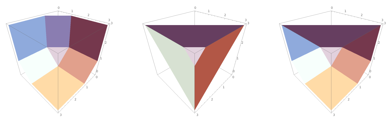
Figure 6: The boundaries of value manifolds for three-class hinge-like losses $L^{\text{DKR2}}$/$L^{\text{zo4}}$ (left), $L^{\text{LLW2}}$ (middle) and $L^{\text{zo3}}$ (right). The triangle polytope in the center of each plot is the value manifold $\mathcal{S}^{\text{zo}}$ for the zero-one loss. The boundary of $\mathcal{S}^{\text{zo}*}$, defined as $\mathcal{S}^{\text{zo}}+\mathbb{R}^{m}_{+}$, is the same as in the left plot.

The following result establishes a general link from the generalized entropy of the zero-one loss to classification regret bounds. The link involves a particular prediction mapping $\sigma_{L}(\gamma)$, defined from the negative values of a given loss $L$. Such a prediction mapping is also exploited to study classification calibration in Tewari and Bartlett (2007), with an additional assumption that the value manifold $\mathcal{S}_{L}$ is symmetric.

Proposition 9.

Suppose that a loss $L(j,\gamma)$ with action space $\mathcal{A}$ induces the same generalized entropy as the zero-one loss. Then for $\eta\in\Delta_{m}$ and $\gamma\in\mathcal{A}$, $m^{-1}B_{L^{\text{zo}}}(\eta,\sigma_{L}(\gamma))\leq B_{L}(\eta,\gamma)$, that is,

$$\frac{1}{m}\left\{\sum_{j=1}^{m}\eta_{j}L^{\text{zo}}(j,\sigma_{L}(\gamma))-H^{\text{zo}}(\eta)\right\}\leq\sum_{j=1}^{m}\eta_{j}L(j,\gamma)-H_{L}(\eta),$$ (51)

where $\sigma_{L}(\gamma)=(-L(1,\gamma),\ldots,-L(m,\gamma))^{\mathrm{\scriptscriptstyle T}}$. Moreover, the loss $L(j,\gamma)$, with the prediction mapping $\sigma_{L}$, is classification calibrated for the zero-one loss.

Proposition 9 provides a theoretical support for our approach in constructing hinge-like losses with the same generalized entropy as the zero-one loss in Section 5.1. The regret bound (51) implies classification calibration similarly as discussed in Section 5.2. Hence our result gives a more concrete sufficient condition for achieving classification calibration than in Tewari and Bartlett (2007), Section 4.

By the nature of the zero-one loss, the regret bound (51) remains valid with $\sigma_{L}(\gamma)$ replaced by another prediction mapping $\sigma(\gamma)$ subject to the monotonicity property that the components in $\sigma(\gamma)$ are in the same order as in $\sigma_{L}(\gamma)$ for any $\gamma\in\mathcal{A}$. Then the regret bounds for $L^{\text{zo3}}$, as a special case of $L^{\text{cw3}}$, and $L^{\text{zo4}}$ in Proposition 7 can be deduced from (51), because the monotonicity property is satisfied by the prediction mappings $\tau^{\dagger}$ and $\tilde{\tau}$ used in (45) and (46). See the Supplement for details. Possible extensions of Proposition 9 to cost-weighted classification can be studied in future work.

6 Regret bounds for proper scoring rules

We return to proper scoring rules and derive classification regret bounds, which compare the regrets of the losses with those of the corresponding zero-one and cost-weighted classification losses, similarly as in Proposition 7 for hinge-like losses. All such bounds are also called surrogate regret bounds, in the sense that the a proper scoring rule or a hinge-like loss can be considered a surrogate criterion for the zero-one or cost-weighted classification loss. Similarly as discussed in Section 5.2, these results provide a quantitative guarantee on classification calibration (Zhang, 2004a; Tewari and Bartlett, 2007).

Compared with hinge-like losses, a potential gain in using proper scoring rules is that classification regret bounds can be obtained with respect to a range of cost-weighted classification losses with different cost matrices $C$ for a proper scoring rule, defined independently of $C$. The cost matrix is involved only to convert an action (in the form of a probability vector) from the scoring rule to a prediction for the cost-weighted classification loss. See Corollary 3. In contrast, for the regret bound (45), the hinge-like loss $L^{\text{cw3}}$ depends on the cost-matrix $C$ used in the classification loss $L^{\text{cw}}$. A similar observation is made by Reid and Williamson (2011, Corollary 28) in two-class settings.

A general basis for deriving regret bounds, applicable to not just scoring rules but arbitrary losses $L(j,\gamma)$ with an action space $\mathcal{A}\subset\mathbb{R}^{m}$, can be seen as

$$\psi(B^{\text{zo}}(\eta,\gamma))\leq B_{L}(\eta,\gamma),$$ (52)

where $B^{\text{zo}}(\eta,\gamma)=B_{L^{\text{zo}}}(\eta,\gamma)$, the regret of the zero-one loss $L^{\text{zo}}(\eta,\gamma)$, and

$$\psi(t)=\inf_{\eta^{\prime}\in\Delta_{m},\gamma^{\prime}\in\mathcal{A}:\,B^{\text{zo}}(\eta^{\prime},\gamma^{\prime})=t}B_{L}(\eta^{\prime},\gamma^{\prime}),\quad t\geq 0.$$

In fact, (52) is a tautology from the definition of $\psi$. Various regret bounds can be obtained by identifying convenient lower bounds of $\psi$. In the two-class setting, the regret for the zero-one loss is $B^{\text{zo}}(\eta,\gamma)=|2\eta_{1}-1|1\{(2\eta_{1}-1)(\gamma_{1}-\gamma_{2})\leq 0\}$ for $\eta=(\eta_{1},\eta_{2})^{\mathrm{\scriptscriptstyle T}}\in\Delta_{2}$ and $\gamma=(\gamma_{1},\gamma_{2})^{\mathrm{\scriptscriptstyle T}}$. For $t>0$, $B^{\text{zo}}(\eta,\gamma)=t$ means $\eta_{1}=(1\pm t)/2$, and hence $\psi(t)$ can be simplified as

$$\psi^{\text{BJM}}(t)=\min\left\{\inf_{\gamma^{\prime}:t(\gamma^{\prime}_{1}-\gamma^{\prime}_{2})\leq 0}B_{L}^{1}\left(\frac{1+t}{2},\gamma^{\prime}\right),\inf_{\gamma^{\prime}:t(\gamma^{\prime}_{1}-\gamma^{\prime}_{2})\geq 0}B_{L}^{1}\left(\frac{1-t}{2},\gamma^{\prime}\right)\right\},$$

where $B_{L}^{1}(\eta_{1},\gamma)$ denotes $B_{L}(\eta,\gamma)$ as a function of $(\eta_{1},\gamma)$. Moreover, $\psi^{\text{BJM}}(t)$ at $t=0$ also satisfies $\psi^{\text{BJM}}(0)=0\leq\psi(0)$. Therefore, (52) holds with $\psi$ replaced by $\psi^{\text{BJM}}$:

$$\psi^{\text{BJM}}(B^{\text{zo}}(\eta,\gamma))\leq B_{L}(\eta,\gamma).$$ (53)

In the multi-class setting, the regret $B^{\text{zo}}(\eta,\gamma)$ does not admit a direct simplification. Nevertheless, our results below for proper scoring rules can be seen as further manipulation of (52) by exploiting the fact that the regret (8) is a Bregman divergence due to the canonical representation (7) for proper scoring rules.

Remark 3.

Replacing $\psi^{\text{BJM}}$ in (53) by the greatest convex lower bound on $\psi^{\text{BJM}}$ (or the Fenchel biconjugate of $\psi^{\text{BJM}}$) recovers the regret bound in Bartlett et al. (2006, Theorem 1) in the symmetric case where $L(1,\gamma)=L(2,-\gamma)$. In general, there is a benefit from such a modification in the setting where covariates are restored, instead of being lifted out in most of our discussion. For a regret bound in the form $\phi(B^{\text{zo}}(\eta,\gamma))\leq B_{L}(\eta,\gamma)$, if $\phi$ is convex, then application of Jensen’s inequality gives

$$\phi\big{[}E\{B^{\text{zo}}(\eta(X),\gamma(X))\}\big{]}\leq E\big{[}\phi\{B^{\text{zo}}(\eta(X),\gamma(X))\}\big{]}$$

$$\leq E\{B_{L}(\eta(X),\gamma(X))\},$$

where $E\{B^{\text{zo}}(\eta(X),\gamma(X))$ and $E\{B_{L}(\eta(X),\gamma(X))\}$ are the average regret over $X$.

6.1 Zero-one classification

Before presenting our general regret bounds for proper scoring rules with respect to cost-weighted classification in Sections 6.2–6.3, we demonstrate novel implications of our general results in the simple but important setting of zero-one classification.

For a proper scoring rule $L(j,q)$, an application of our regret bound (65) or (69) with respect to the zero-one loss with $C_{0}=1_{m}$ shows that for any $\eta,q\in\Delta_{m}$,

$$\underline{\psi}\left(B^{\text{zo}}(\eta,q)\right)\leq B_{L}(\eta,q),$$ (54)

where $\underline{\psi}(\cdot)$ is defined as

$$\underline{\psi}(t)=\inf_{\begin{subarray}{c}\eta^{\prime},q^{\prime}\in\Delta_{m}:\,\|\eta^{\prime}-q^{\prime}\|_{\infty 2}=t,\\ \max_{j\in[m]}q^{\prime}_{j}\leq 1/2\end{subarray}}B_{L}(\eta^{\prime},q^{\prime}),\quad t\geq 0.$$ (55)

For a vector $b=(b_{1},\ldots,b_{m})^{\mathrm{\scriptscriptstyle T}}$, $\|b\|_{\infty 2}$ denotes $\max_{j\not=k\in[m]}$ $(|b_{j}|+|b_{k}|)$. Inequality (54) can be seen to extend the two-class regret bound (53) in Bartlett et al. (2006) to multi-class settings for proper scoring rules. Unlike the two-class setting, additional effort is needed to find a simple meaningful lower bound of $\underline{\psi}$ in the multi-class setting. Our current approach involves deriving a lower bound on the regret (or Bregman divergence) $B_{L}$ by the $L_{1}$ norm, such that for any $\eta,q\in\Delta_{m}$,

$$B_{L}(\eta,q)=H_{L}(q)-H_{L}(\eta)-(q-\eta)^{\mathrm{\scriptscriptstyle T}}\partial H_{L}(q)\geq\frac{\kappa_{L}}{2}\|\eta-q\|_{1}^{2},$$ (56)

where $\kappa_{L}>0$ is a constant depending on $L$, and $\|b\|_{1}=\sum_{j=1}^{m}|b_{j}|$ is the $L_{1}$ norm for any vector $b=(b_{1},\ldots,b_{m})^{\mathrm{\scriptscriptstyle T}}$. Hence (56) can be interpreted as saying that $-H_{L}$ is strongly convex with respect to the $L_{1}$ norm with modulus $\kappa_{L}$. Because $\|\eta-q\|_{1}\geq\|\eta-q\|_{\infty 2}$, the regret bound (54) together with (56) implies that for any $\eta,q\in\Delta_{m}$,

$$\frac{\kappa_{L}}{2}\left(B^{\text{zo}}(\eta,q)\right)^{2}\leq B_{L}(\eta,q).$$ (57)

In general, the preceding discussion shows that a lower bound on the Bregman divergence $B_{L}(\eta,q)$ by some norm of $\eta-q$ can be translated into a corresponding regret bound.

Our current approach does not exploit the restriction that $\max_{j\in[m]}q_{j}^{\prime}\leq 1/2$ in the definition of $\underline{\psi}$. Hence it is interesting to study how our results here can be improved. On the other hand, such an improvement, even if achieved, may be limited. See the later discussion on regret bounds for the pairwise exponential loss.

Our approach leads to the following result for two classes of proper scoring rules discussed in Section 4: a class of pairwise losses (29) with $f_{0}$ associated with a Beta family of weight functions as studied in Buja et al. (2005), and a class of simultaneous losses (33). In all these cases, inequalities (56) can be of independent interest.

Proposition 10.

Inequalities (56) and (57) hold for the following proper scoring rules.

• Consider a pairwise loss $L=L_{f_{0}}^{\text{pw,s}}$ in (29), with a univariate function $f_{0}$ defined such that (27) holds with a weight function $w(q_{1})=2^{2\nu}q_{1}^{\nu-1}q_{2}^{\nu-1}$ for $(q_{1},q_{2})^{\mathrm{\scriptscriptstyle T}}\in\Delta_{2}$. If $\nu\leq 0$, then (56) and (57) are valid with $\kappa_{L}=2$.

• Consider a simultaneous loss $L=L_{\beta}$ in (33). Then (56) and (57) are valid with

  $$\kappa_{L}=\left\{\begin{array}[]{cl}(1-\beta)m^{(1-1/\beta)(2\beta-1)}2^{2-2\beta},&\mbox{if }\beta\in[1/2,1),\\ (1-\beta)2^{1/\beta-1},&\mbox{if }\beta\in(0,1/2].\end{array}\right.$$

  The bounds from the two segments both give $\kappa_{L}=1$ at $\beta=1/2$.

We discuss several specific examples. The standard likelihood loss $L(j,q)=-\log q_{j}$ is equivalent to the simultaneous loss $L_{\beta}$ in the limit of $\beta\to 1$ after properly rescaled. In this case, Pinsker’s inequality states that (56) holds with $\kappa_{L}=1$ (Cover and Thomas, 1991, Lemma 12.6.1):

$$\sum_{j=1}^{m}\eta_{j}\log(\eta_{j}/q_{j})\geq\frac{1}{2}\left(\sum_{j=1}^{m}|\eta_{j}-q_{j}|\right)^{2}.$$ (58)

The resulting regret bound (57) for the standard likelihood loss $L$ then gives

$$\frac{1}{2}\left(B^{\text{zo}}(\eta,q)\right)^{2}\leq B_{L}(\eta,q).$$ (59)

This surrogate regret bound for the multinomial likelihood appears new, even though the Bregman divergence bound (58) is known. In the Supplement, we verify that (58) can be recovered from (56) using Proposition 10(ii).

The pairwise exponential loss associated with multi-class boosting is defined equivalently as $L_{e}^{\text{pw,s}}(j,q)=2(L_{1/2}-1)=2\sum_{k\in[m],k\not=j}\sqrt{q_{k}/q_{j}}$ in Section 2.2. The two inequalities (56) obtained from Proposition 10, part (i) with $\nu=-1/2$ and part (ii) with $\beta=1/2$, are equivalent to each other and both lead to

$$H_{L_{1/2}}(q)-H_{L_{1/2}}(\eta)-(q-\eta)^{\mathrm{\scriptscriptstyle T}}\partial H_{L_{1/2}}(q)\geq\frac{1}{2}\|\eta-q\|_{1}^{2},$$ (60)

where $H_{1/2}(q)=\|q\|_{1/2}$ and $L_{1/2}(j,q)=(\|q\|_{1/2}/q_{j})^{1/2}=\sum_{k=1}^{m}\sqrt{q_{k}/q_{j}}$. The resulting regret bound (57) for the rescaled pairwise exponential loss $L_{1/2}$ gives

$$\frac{1}{2}\left(B^{\text{zo}}(\eta,q)\right)^{2}\leq B_{L_{1/2}}(\eta,q).$$ (61)

The two bounds (59) and (61) for the likelihood and rescaled pairwise exponential losses happen to be of the same form, due to the scaling used. For the two-class exponential loss defined as $L_{e}=L_{1/2}-1$, the existing regret bound (53), corresponding to an exact calculation of $\underline{\psi}$ by the proof of (70) later, is

$$1-\sqrt{1-(B^{\text{zo}}(\eta,q))^{2}}\leq B_{L_{1/2}}(\eta,q),$$

which is slightly stronger than (61) because $1-\sqrt{1-\delta^{2}}\geq\delta^{2}/2$ for $\delta\in[0,1]$, but $(1-\sqrt{1-\delta^{2}})/(\delta^{2}/2)\to 1$ as $\delta\to 0$. Therefore, our result (61) provides a reasonable extension of existing regret bounds to multi-class pairwise exponential losses.

A notable proper scoring rule which is not informed by Proposition 10 for $m\geq 3$ is the simultaneous exponential loss $L^{\text{r}}_{0}$ as used in Zou et al. (2008), even though the loss $L^{\text{r}}_{0}$ is equivalent to the exponential loss for $m=2$. See the Supplement for details.

Remark 4.

Inequality (56) on the Bregman divergence in general differs from generalized Pinsker inequalities relating (two-distribution) $f$-divergences to the total variation studied in Reid and Williamson (2011), Section 7.2, for binary experiments. For the pairwise exponential loss, the Bregman divergence on the left-hand side of (60) can be calculated as $(\sum_{j\in[m]}\sqrt{q_{j}})(\sum_{j\in[m]}\eta_{j}/\sqrt{q_{j}})-(\sum_{j\in[m]}\sqrt{\eta_{j}})^{2}$, which is apparently not any $f$-divergence between probability vectors $\eta$ and $q$. An exception is the classical Pinsker inequality (58): the Kullback–Liebler divergence on the left-hand side of (58) is both an $f$-divergence with $f(t)=t\log t$ and a Bregman divergence with $H_{L}(\eta)=-\sum_{j\in[m]}\eta_{j}\log\eta_{j}$.

Remark 5.

In the two-class setting, a scoring rule satisfying inequality (56) is called a strongly proper loss, and surrogate regret bounds are obtained for strongly proper losses with respect to the area under the curve (AUC) in Agarwal (2013). It is interesting to investigate possible extensions of such results to the multi-class setting.

6.2 Cost-transformed losses

We study two types of classification regret bounds with respect to a general cost-weighted classification loss as defined in Section 2.3. This subsection deals with the first type where a classification regret bound is derived for a loss, allowed to depend on a pre-specified cost matrix $C$, similarly as the hinge-like loss $L^{\text{cw3}}$ in (42). An action of the loss is directly taken as a prediction for the cost-weighted classification loss. See the next subsection on the second type of classification regret bounds.

For a general loss $L(j,\gamma)$ (not just scoring rules), define a cost-transformed loss, depending on a cost matrix $C$, as

$$\tilde{L}(j,\gamma)=c_{jM}L(j,\gamma)+\sum_{k\in[m],k\not=j}(c_{jM}-c_{jk})\{L(k,\gamma)-1\},$$ (62)

where $c_{jM}=\max_{k\in[m]}c_{jk}$. In the special case where $C=1_{m}1_{m}^{\mathrm{\scriptscriptstyle T}}-I_{m}$ for the zero-one loss, the transformed loss $\tilde{L}(j,\gamma)$ reduces to the original loss $L(j,\gamma)$. A motivation for this construction is that the cost-weighted classification loss can also be obtained in this way from the zero-one loss: $L^{\text{cw}}(j,\gamma)=\tilde{L}^{\text{zo}}(j,\gamma)$. In general, the risk and regret of the transformed loss can be related to those of the original loss as follows.

Lemma 4.

The risks of the losses $\tilde{L}(j,\gamma)$ and $L(j,\gamma)$ satisfy

$$R_{\tilde{L}}(\eta,\gamma)=(1_{m}^{\mathrm{\scriptscriptstyle T}}\tilde{\eta})\,R_{L}(\tilde{\tilde{\eta}},\gamma)-D(\eta),$$

where $D(\eta)=\sum_{j\in[m]}\sum_{k\in[m],k\not=j}\eta_{j}(c_{jM}-c_{jk})$, $\tilde{\tilde{\eta}}=\tilde{\eta}/(1_{m}^{\mathrm{\scriptscriptstyle T}}\tilde{\eta})\in\Delta_{m}$, and $\tilde{\eta}=(\tilde{\eta}_{1},\ldots,\tilde{\eta}_{m})^{\mathrm{\scriptscriptstyle T}}$ $\in\mathbb{R}^{m}_{+}$ with

$$\tilde{\eta}_{j}=c_{jM}\eta_{j}+\sum_{k\in[m],k\not=j}(c_{kM}-c_{kj})\eta_{k}.$$

Moreover, the regrets of $\tilde{L}$ and $L$ satisfy $B_{\tilde{L}}(\eta,\gamma)=(1_{m}^{\mathrm{\scriptscriptstyle T}}\tilde{\eta})\,B_{L}(\tilde{\tilde{\eta}},\gamma)$.

For a scoring rule $L(j,q)$ with actions defined as probability vectors $q\in\Delta_{m}$, there is a simple upper bound on the regret of the associated zero-one loss $L^{\text{zo}}(j,q)$, which is instrumental to our derivation of classification regret bounds.

Lemma 5.

For any $\eta,q\in\Delta_{m}$, it holds that

$$B^{\text{zo}}(\eta,q)\leq\|\eta-q\|_{\infty 2},$$

where $\|b\|_{\infty 2}=\max_{j\not=k\in[m]}$ $(|b_{j}|+|b_{k}|)$ for any vector $b=(b_{1},\ldots,b_{m})^{\mathrm{\scriptscriptstyle T}}$. The bound is tight for any $m\geq 2$ in that there exist $\eta,q\in\Delta_{m}$ for which the bound becomes exact.

Combining the preceding two lemmas and invoking a similar argument as indicated by (52) leads to the following regret bound, depending on the action $q$.

Proposition 11.

For a scoring rule $L(j,q)$, define a nondecreasing function $\psi_{q}$:

$$\psi_{q}(t)=\inf_{\eta^{\prime}\in\Delta_{m}:\|\eta^{\prime}-q\|_{\infty 2}\geq t}B_{L}(\eta^{\prime},q),\quad t\geq 0.$$

Then the regrets of the cost-weighted classification loss $L^{\text{cw}}(j,q)$ and the cost-transformed scoring rule $\tilde{L}(j,q)$ satisfy

$$\psi_{q}\left(\frac{B^{\text{cw}}(\eta,q)}{1_{m}^{\mathrm{\scriptscriptstyle T}}\tilde{\eta}}\right)\leq\frac{B_{\tilde{L}}(\eta,q)}{1_{m}^{\mathrm{\scriptscriptstyle T}}\tilde{\eta}},$$ (63)

where $B^{\text{cw}}=B_{L^{\text{cw}}}$, and $\tilde{\eta}$ is defined, depending on $\eta$ and $C$, as in Lemma 4.

A cost-transformed loss (62) from a proper scoring rule can be easily shown to remain a proper scoring rule. In this case, a uniform regret bound can be obtained from (63), by taking an infimum over $q$ and incorporating simplification due to the representation of the regret (8) as a Bregman divergence for a proper scoring rule.

Corollary 2.

For a proper scoring rule $L(j,q)$, the regrets of $L^{\text{cw}}(j,q)$ and $\tilde{L}(j,q)$ satisfy

$$\underline{\psi}\left(\frac{B^{\text{cw}}(\eta,q)}{1_{m}^{\mathrm{\scriptscriptstyle T}}\tilde{\eta}}\right)\leq\frac{B_{\tilde{L}}(\eta,q)}{1_{m}^{\mathrm{\scriptscriptstyle T}}\tilde{\eta}},$$ (64)

where $\underline{\psi}$ is defined in (55), and $\tilde{\eta}$ is defined, depending on $\eta$ and $C$, in Lemma 4.

It is instructive to examine the regret bound (64) in the special case of class-weighted costs, where $C=C_{0}1_{m}^{\mathrm{\scriptscriptstyle T}}-\mathrm{diag}(C_{0})$ with $C_{0}=(c_{10},\ldots,c_{m0})^{\mathrm{\scriptscriptstyle T}}$. The cost-transformed loss $\tilde{L}$ reduces to $\tilde{L}(j,q)=c_{j0}L(j,q)$. The regret bound (64) becomes

$$\underline{\psi}\left(\frac{B^{\text{cw0}}(\eta,q)}{C_{0}^{\mathrm{\scriptscriptstyle T}}\eta}\right)\leq\frac{B_{\tilde{L}}(\eta,q)}{C_{0}^{\mathrm{\scriptscriptstyle T}}\eta},$$ (65)

where $B^{\text{cw0}}=B_{L^{\text{cw0}}}$. We defer a discussion of these results until after Corollary 3.

6.3 Cost-independent losses

We derive a different type of classification regret bounds than in the preceding subsection. Here a loss used for training is defined independently of any cost matrix, but an action of the loss can be converted after training to a prediction, depending on the cost matrix $C$, for the cost-weighted classification loss. For scoring rules, our derivation relies on the following extension of Lemma 5 on the regret of the cost-weighted classification loss, where a prediction is linearly converted from a probability vector.

Lemma 6.

For any $\eta,q\in\Delta_{m}$, it holds that

$$B^{\text{cw}}(\eta,\overline{C}^{\mathrm{\scriptscriptstyle T}}q)\leq\|\overline{C}^{\mathrm{\scriptscriptstyle T}}(\eta-q)\|_{\infty 2},$$

where $\overline{C}=C_{M}1_{m}^{\mathrm{\scriptscriptstyle T}}-C$ and $C_{M}=(c_{1M},\ldots,c_{mM})^{\mathrm{\scriptscriptstyle T}}$ with $c_{jM}=\max_{k\in[m]}c_{jk}$ for $j\in[m]$ as defined in the transformed loss (62).

By a similar argument as indicated by (52), we obtain a regret bound which compares the regret of a scoring rule $L(j,q)$ with that of the cost-weighted classification loss with a prediction depending on both $q$ and $C$ as in Lemma 6.

Proposition 12.

For a scoring rule $L(j,q)$, define a nondecreasing function $\psi_{q}^{C}$:

$$\psi_{q}^{C}(t)=\inf_{\eta^{\prime}\in\Delta_{m}:\|\overline{C}^{\mathrm{\scriptscriptstyle T}}(\eta^{\prime}-q)\|_{\infty 2}\geq t}B_{L}(\eta^{\prime},q),\quad t\geq 0.$$

Then the regrets of the cost-weighted classification loss $L^{\text{cw}}(j,\overline{C}^{\mathrm{\scriptscriptstyle T}}q)$ and the scoring rule $L(j,q)$ satisfy

$$\psi_{q}^{C}\left(B^{\text{cw}}(\eta,\overline{C}^{\mathrm{\scriptscriptstyle T}}q)\right)\leq B_{L}(\eta,q).$$ (66)

For a proper scoring rule $L(j,q)$, the regret bound (66) can be strengthened (see the Supplement for a proof) such that for each $w\in\mathcal{W}_{\eta,q}$,

$$\psi^{C}_{q^{w}}\left(B^{\text{cw}}(\eta,\overline{C}^{\mathrm{\scriptscriptstyle T}}q)\right)\leq B_{L}(\eta,q),$$ (67)

where $q^{w}=(1-w)\eta+wq$ and

$$\mathcal{W}_{\eta,q}=\left\{w\in[0,1]:\overline{C}^{\mathrm{\scriptscriptstyle T}}_{k}q^{w}=\max_{j}(\overline{C}^{\mathrm{\scriptscriptstyle T}}_{j}q^{w})\mbox{ for }k=\mathrm{argmax}_{j}(\overline{C}^{\mathrm{\scriptscriptstyle T}}_{j}q)\right\}\ni 1.$$

By definition, $w\in\mathcal{W}_{\eta,q}$ means that using $q^{w}$ yields the same classification as using $q$. Moreover, a uniform regret bound can be obtained from (67) by minimizing over $q^{w}$ with $w\in\mathcal{W}_{\eta,q}$ such that $\max_{j\in[m]}\overline{C}^{\mathrm{\scriptscriptstyle T}}_{j}q^{w}\leq 1_{m}^{\mathrm{\scriptscriptstyle T}}\overline{C}^{\mathrm{\scriptscriptstyle T}}q^{w}/2$.

Corollary 3.

For a proper scoring rule $L(j,q)$, define

$$\underline{\psi}^{C}(t)=\inf_{\begin{subarray}{c}\eta^{\prime},q^{\prime}\in\Delta_{m}:\,\|\overline{C}^{\mathrm{\scriptscriptstyle T}}(\eta^{\prime}-q^{\prime})\|_{\infty 2}=t,\\ \max_{j\in[m]}(\overline{C}_{j}^{\mathrm{\scriptscriptstyle T}}q^{\prime})\leq 1_{m}^{\mathrm{\scriptscriptstyle T}}\overline{C}^{\mathrm{\scriptscriptstyle T}}q^{\prime}/2\end{subarray}}B_{L}(\eta^{\prime},q^{\prime}),\quad t\geq 0.$$

Then the regrets of $L^{\text{cw}}(j,\overline{C}^{\mathrm{\scriptscriptstyle T}}q)$ and $L(j,q)$ satisfy

$$\underline{\psi}^{C}\left(B^{\text{cw}}(\eta,\overline{C}^{\mathrm{\scriptscriptstyle T}}q)\right)\leq B_{L}(\eta,q).$$ (68)

In the special case of class-weighted costs, corresponding to $C=C_{0}1_{m}^{\mathrm{\scriptscriptstyle T}}-\mathrm{diag}(C_{0})$ with $C_{0}=(c_{10},\ldots,c_{m0})^{\mathrm{\scriptscriptstyle T}}$, define

$$\underline{\psi}^{C_{0}}(t)=\inf_{\begin{subarray}{c}\eta^{\prime},q^{\prime}\in\Delta_{m}:\,\|C_{0}\circ(\eta^{\prime}-q^{\prime})\|_{\infty 2}=t,\\ \max_{j\in[m]}(c_{j0}q^{\prime}_{j})\leq C_{0}^{\mathrm{\scriptscriptstyle T}}q^{\prime}/2\end{subarray}}B_{L}(\eta^{\prime},q^{\prime}),\quad t\geq 0,$$

where $\circ$ denotes the component-wise product between two vectors. The regret bound (68) for proper scoring rules reduces to

$$\underline{\psi}^{C_{0}}\left(B^{\text{cw0}}(\eta,C_{0}\circ q)\right)\leq B_{L}(\eta,q).$$ (69)

It is interesting to compare the two regret bounds (65) and (69). On one hand, for the zero-one loss with $C_{0}=1_{m}$, both of these bounds lead to the regret bound (54) discussed in Section 6.1. On the other hand, the two bounds (65) and (69) in general serve different purposes. The bound (65) compares the regrets of the transformed scoring rule $\tilde{L}$ depending on $C_{0}$ and the classification loss $L^{\text{cw0}}$ with the prediction always set to $q$. To use $\tilde{L}$, a different round of training is required for a different choice of $C_{0}$. The bound (69) relates the regrets of the original scoring rule $L$, independent of $C_{0}$, and the classification loss $L^{\text{cw0}}$ with the prediction defined as $C_{0}\circ q$. Only one round of training is needed to determine $q$ when using $L$, and then the prediction can be adjusted from $q$ according to the choice of $C_{0}$. Hence the bound (69) can be potentially more useful than (65).

For binary classification with $m=2$, the regret bound (69) for proper scoring rules can be shown to recover Theorem 25 in Reid and Williamson (2011). For a proper scoring rule $L(j,q)$ and any $\eta,q\in\Delta_{2}$, it holds that

$$\min\left\{\psi^{\text{RW}}(\delta),\psi^{\text{RW}}(-\delta)\right\}\leq B_{L}(\eta,q),$$ (70)

where $\delta=B^{\text{cw0}}(\eta,C_{0}\circ q)$, $\psi^{\text{RW}}(\delta)=B_{L}^{1}((c_{20}+\delta)/(c_{10}+c_{20}),c_{20}/(c_{10}+c_{20}))$, and $B_{L}^{1}(\eta_{1},q_{1})=B_{L}(\eta,q)$ with $\eta=(\eta_{1},\eta_{2})^{\mathrm{\scriptscriptstyle T}}$ and $q=(q_{1},q_{2})^{\mathrm{\scriptscriptstyle T}}$, that is, $B_{L}^{1}(\eta_{1},q_{1})$ is $B_{L}(\eta,q)$ treated as a function of $(\eta_{1},q_{1})$ only. See the Supplement for details.

7 Conclusion

In this article, we are mainly concerned with constructing losses and establishing corresponding regret bounds in multi-class settings. Various topics are of interest for further research. Large sample theory can be studied regarding estimation and approximation errors, similarly as in Zhang (2004b) and Bartlett et al. (2006), by taking advantage of our multi-class regret bounds. Computational algorithms need to be developed for implementing our new hinge-like losses and, in connection with boosting algorithms, for implementing composite losses based on new proper scoring rules. Numerical experiments are also desired to evaluate empirical performance of new methods.

I Technical details

I.1 Preparation

For a convex function $\psi$ defined on a convex domain $\Omega$, the Bregman divergence is defined as

$$B_{\psi}(x,y)=\psi(x)-\psi(y)-(x-y)^{\mathrm{\scriptscriptstyle T}}\partial\psi(y),$$

where $\partial\psi$ is a sub-gradient of $\psi$. The symmetrized Bregman divergence is

$$B_{\psi}(x,y)+B_{\psi}(y,x)=(y-x)^{\mathrm{\scriptscriptstyle T}}\{\partial\psi(y)-\partial\psi(x)\}.$$

The following lemma shows that the Bregman divergence is nondecreasing as the first (or second) argument, $x$ or $y$, moves away from the other argument, $y$ or $x$, along a straight line, while the second (or respectively first) argument remains fixed.

Lemma S1.

For any $x,y\in\Omega$ and $w\in[0,1]$, we have

$$B_{\psi}(x,y)\geq B_{\psi}(x^{w},y),$$ (S1)

$$B_{\psi}(x,y)\geq B_{\psi}(x,x^{w}).$$ (S2)

where $x^{w}=(1-w)x+wy$.

Proof. If $w=0$ or 1, then (S1) and (S2) hold trivially. In the following, assume $w\in(0,1)$. To show (S1), direct calculation yields

$$B_{\psi}(x,y)-B_{\psi}(x^{w},y)=\psi(x)-\psi(x^{w})-(x-x^{w})^{\mathrm{\scriptscriptstyle T}}\partial\psi(y)$$

$$=B_{\psi}(x,x^{w})+(x-x^{w})^{\mathrm{\scriptscriptstyle T}}\{\partial\psi(x^{w})-\partial\psi(y)\}$$

$$=B_{\psi}(x,x^{w})+\frac{w}{1-w}(x^{w}-y)^{\mathrm{\scriptscriptstyle T}}\{\partial\psi(x^{w})-\partial\psi(y)\}.$$

Hence (S1) follows because $(x^{w}-y)^{\mathrm{\scriptscriptstyle T}}\{\partial\psi(x^{w})-\partial\psi(y)\}$ is the symmetrized Bregman divergence between $x^{w}$ and $y$. From the preceding equations, we see

$$B_{\psi}(x,y)-B_{\psi}(x,x^{w})=B_{\psi}(x^{w},y)+\frac{w}{1-w}(x^{w}-y)^{\mathrm{\scriptscriptstyle T}}\{\partial\psi(x^{w})-\partial\psi(y)\}.$$

Hence (S2) follows because $(x^{w}-y)^{\mathrm{\scriptscriptstyle T}}\{\partial\psi(x^{w})-\partial\psi(y)\}\geq 0$ again. $\blacksquare$

I.2 Proofs of results in Section 3

Proof of Proposition 2.  Denote by $\partial^{\dagger}f$ the set of all sub-gradients of $f$. For any $u\in\overline{\mathbb{R}}_{+}^{m-1}$ and $s=\partial f(u)\in\partial^{\dagger}f(u)$, Fenchel’s conjugacy property implies that $f^{*}(s)=u^{\mathrm{\scriptscriptstyle T}}s-f(u)$ and hence $s\in\mathrm{dom}(f^{*})$. Moreover, we have

$$\sum_{j=1}^{m}\eta_{j}L_{f2}(j,u)=\sum_{j=1}^{m-1}\eta_{j}(-\partial_{j}f(u))+\eta_{m}(u^{\mathrm{\scriptscriptstyle T}}\partial f(u)-f(u))$$

$$\quad=\sum_{j=1}^{m-1}(-\eta_{j}s_{j})+\eta_{m}f^{*}(s)=\sum_{j=1}^{m}\eta_{j}L_{f}(j,s).$$

Therefore,

$$\inf_{u\in\overline{\mathbb{R}}_{+}^{m-1}}\left\{\sum_{j=1}^{m}\eta_{j}L_{f2}(j,u)\right\}\geq\inf_{s\in\mathrm{dom}(f^{*})}\left\{\sum_{j=1}^{m}\eta_{j}L_{f}(j,s)\right\}=H_{f}(\eta).$$

Next, we show the reverse inequality. For any $\eta\in\Delta_{m}$, denote $u^{\eta}=(\eta_{1}/\eta_{m},\ldots,\eta_{m-1}/\eta_{m})^{\mathrm{\scriptscriptstyle T}}$ and $s^{\eta}=\partial f(u^{\eta})\in\partial^{\dagger}f(u^{\eta})$. Then

$$H_{f}(\eta)=-\eta_{m}f(u^{\eta})=-\eta_{m}\left\{\sum_{j=1}^{m-1}u_{j}^{\eta}s_{j}^{\eta}-f^{*}(s^{\eta})\right\}$$

$$=\sum_{j=1}^{m-1}(-\eta_{j}s_{j}^{\eta})+\eta_{m}f^{*}(s^{\eta})=\sum_{j=1}^{m-1}\eta_{j}(-\partial_{j}f(u^{\eta}))+\eta_{m}(u^{\eta{\mathrm{\scriptscriptstyle T}}}\partial f(u^{\eta})-f(u^{\eta})),$$

where Fenchel’s conjugacy property, $u^{\eta{\mathrm{\scriptscriptstyle T}}}s^{\eta}=f(u^{\eta})+f^{*}(s^{\eta})$, is used in the last equalities on the first and second lines. Hence $H_{f}(\eta)\geq\inf_{u\in\overline{\mathbb{R}}_{+}^{m-1}}\{\sum_{j=1}^{m}\eta_{j}L_{f2}(j,u)\}$. $\blacksquare$

Proof of equation (25).  By definition, $H_{f}(q)=-q_{m}f(q_{1}/q_{m},\ldots,q_{m-1}/q_{m})$. The sub-gradient of $-H_{f}$ can be calculated as

$$-\partial_{j}H_{f}(q_{1},\ldots,q_{m})=\left\{\begin{array}[]{cl}\partial_{j}f(u^{q}),&\mbox{if }j\in[m-1],\\ f(u^{q})-\sum_{j=1}^{m-1}\frac{q_{j}}{q_{m}}\partial_{j}f(u^{q}),&\mbox{if }j=m,\end{array}\right.$$

where $u^{q}=(q_{1}/q_{m},\ldots,q_{m-1}/q_{m})^{\mathrm{\scriptscriptstyle T}}$. Substituting these expressions into $H_{f}(q)-\sum_{j=1}^{m}(q_{j}-\eta_{j})\partial_{j}H_{f}(q)$ yields the second equality in Eq. (25):

$$H_{f}(q)-\sum_{j=1}^{m}(q_{j}-\eta_{j})\partial_{j}H_{f}(q)$$

$$=-q_{m}f(u^{q})+\sum_{j=1}^{m-1}(q_{j}-\eta_{j})\partial_{j}f(u^{q})+(q_{m}-\eta_{m})\left\{f(u^{q})-\sum_{j=1}^{m-1}\frac{q_{j}}{q_{m}}\partial_{j}f(u^{q})\right\}$$

$$=-\sum_{j=1}^{m-1}\eta_{j}\partial_{j}f(u^{q})+\eta_{m}\left\{-f(u^{q})+\sum_{j=1}^{m-1}\frac{q_{j}}{q_{m}}\partial_{j}f(u^{q})\right\}.$$

$\blacksquare$

I.3 Proofs of results in Section 4

Proof of equation (29).  By manipulating the summation, we have

$$L_{f_{0}}^{\text{pw,s}}(j,q)=\sum_{l,k\in[m],k\not=l}\left[-\mathbbm{1}_{k}(j)\partial f_{0}(\frac{q_{k}}{q_{l}})+\mathbbm{1}_{l}(j)\left\{\frac{q_{k}}{q_{l}}\partial f_{0}(\frac{q_{k}}{q_{l}})-f_{0}(\frac{q_{k}}{q_{l}})\right\}\right]$$

$$=\sum_{l\in[m]}\sum_{k\in[m],k\not=l}\left\{-\mathbbm{1}_{k}(j)\partial f_{0}(\frac{q_{k}}{q_{l}})\right\}+\sum_{k\in[m]}\sum_{l\in[m],l\not=k}\mathbbm{1}_{l}(j)\left\{\frac{q_{k}}{q_{l}}\partial f_{0}(\frac{q_{k}}{q_{l}})-f_{0}(\frac{q_{k}}{q_{l}})\right\}$$

$$=\sum_{l\in[m],j\not=l}\left\{-\partial f_{0}(\frac{q_{j}}{q_{l}})\right\}+\sum_{k\in[m],j\not=k}\left\{\frac{q_{k}}{q_{j}}\partial f_{0}(\frac{q_{k}}{q_{j}})-f_{0}(\frac{q_{k}}{q_{j}})\right\},$$

which yields the desired result. $\blacksquare$

Convexity of two-class composite losses.  Consider a logistic link $q^{h_{0}}=(q_{1}^{h_{0}},q_{2}^{h_{0}})^{\mathrm{\scriptscriptstyle T}}$, where $q_{1}^{h_{0}}=\{1+\exp(-h_{0})\}^{-1}$ or equivalently $q_{1}^{h_{0}}/q_{2}^{h_{0}}=\exp(h_{0})$. Then it can be easily shown that the three composite losses, $L_{\ell}(j,q^{h_{0}})$, $L_{e}(j,q^{h_{0}})$, and $L_{c}(j,q^{h_{0}})$, are convex in $h_{0}$, with the following gradients:

$$\frac{\mathrm{d}}{\mathrm{d}h_{0}}L_{\ell}(j,q^{h_{0}})=-\left\{\mathbbm{1}_{1}(j)-q_{1}^{h_{0}}\right\},$$

$$\frac{\mathrm{d}}{\mathrm{d}h_{0}}L_{e}(j,q^{h_{0}})=-\left\{\mathbbm{1}_{1}(j)-q_{1}^{h_{0}}\right\}(q_{2}^{h_{0}}q_{1}^{h_{0}})^{-1/2},$$

$$\frac{\mathrm{d}}{\mathrm{d}h_{0}}L_{c}(j,q^{h_{0}})=-\left\{\mathbbm{1}_{1}(j)/q_{1}^{h_{0}}-1\right\}/2.$$

The corresponding weight functions are in the Beta family, $w(q_{1})=2^{\nu_{1}+\nu_{2}}q_{1}^{\nu_{1}-1}q_{2}^{\nu_{2}-1}$, with $(\nu_{1},\nu_{2})=(0,0),(-1/2,-1/2)$ and $(-1,0)$ respectively. As discussed in Buja et al. (2005, Section 15), a proper scoring rule with a logistic link and $w(q_{1})$ in the Beta family is convex in $h_{0}$ if and only if $\nu_{1},\nu_{2}\in[-1,0]$. Hence the likelihood and calibration losses are at the boundary of achieving convexity in $h_{0}$. $\blacksquare$

Proof of Proposition 4.  The scoring rules are obtained directly from Proposition 3. First, we show the three limits of $H_{\beta}$ for $\beta=0,1,\infty$.

(i) Rewrite $H_{\beta}(q)$ as

$$H_{\beta}(q) =\frac{\exp\{\frac{1}{\beta}\log(1+\frac{\sum_{j=1}^{m}(q_{j}^{\beta}-1)}{m})\}-m^{-\frac{1}{\beta}}}{m^{-1}-m^{-\frac{1}{\beta}}}.$$

Using $\log(1+x)/x\to 1$ as $x\rightarrow 0$, we have

$$\lim_{\beta\to 0+}H_{\beta}(q) =\lim_{\beta\to 0+}\frac{\exp\{\frac{\sum_{j=1}^{m}(q_{j}^{\beta}-1)}{\beta m}\}-m^{-\frac{1}{\beta}}}{m^{-1}-m^{-\frac{1}{\beta}}}=m\left(\prod_{j=1}^{m}q_{j}\right)^{\frac{1}{m}},$$

where the last step holds because $\lim_{\beta\rightarrow 0+}(q_{j}^{\beta}-1)/\beta=\log q_{j}$ by L’Hopital’s rule.

(iii) Rewrite $H_{\beta}(q)$ as

$$H_{\beta}(q) =\frac{\exp\{\frac{1}{\beta}\log(\sum_{j=1}^{m}q_{j}^{\beta})\}-1}{\exp\{(\frac{1}{\beta}-1)\log m\}-1}.$$

Using $(\mathrm{e}^{x}-1)/x\to 1$ as $x\rightarrow 0$, we obtain

$$\lim_{\beta\to 1}H_{\beta}(q) =\lim_{\beta\to 1}\frac{\log(\sum_{j=1}^{m}q_{j}^{\beta})}{(1-\beta)\log m}.$$

Applying L’Hopital’s rule yields

$$\lim_{\beta\rightarrow 1}H_{\beta}(q)=\lim_{\beta\rightarrow 1}\frac{-\sum_{j=1}^{m}q_{j}^{\beta}\log q_{j}}{(\log m)(q_{1}^{\beta}+\dots+q_{m}^{\beta})}=\frac{-\sum_{j=1}^{m}q_{j}\log q_{j}}{\log m}.$$

(iv) The result follows from the standard limit of $L^{p}$-norm, $\lim_{p\rightarrow\infty}\|x\|_{p}=\|x\|_{\infty}$, where $\|x\|_{p}=(\sum_{j=1}^{m}|x_{j}|^{p})^{1/p}$ and $\|x\|_{\infty}=\max_{j\in[m]}|x_{j}|$ for $x\in\mathbb{R}^{m}$.

Finally, we show that the composite loss $L^{\text{r}}_{\beta}(j,q^{h})$ is convex in $h$ for $\beta\in[0,1]$. The case $\beta=0$ or 1 can be verified directly, corresponding to the simultaneous exponential or likelihood composite loss. For $\beta\in(0,1)$, the unscaled composite loss $L_{\beta}(j,q^{h})$ is

$$L_{\beta}(j,q^{h})=\left\{1+\sum_{i\neq j}\exp(\beta(h_{i}-h_{j}))\right\}^{\frac{1}{\beta}-1}.$$

It suffices to show that for $\beta\in(0,1)$, the function

$$g(x)=\left\{1+\sum_{i=1}^{m-1}\exp(\beta x_{i})\right\}^{\frac{1}{\beta}-1}$$

is convex in $x\in\mathbb{R}^{m-1}$. Rewrite $g(x)$ as

$$g(x)=\exp\left[\left(\frac{1}{\beta}-1\right)\log\left\{1+\sum_{i=1}^{m-1}\exp(\beta x_{i})\right\}\right].$$

Note that $\log\{1+\sum_{i=1}^{m-1}\exp(\beta x_{i})\}$ is convex in $x$ (Boyd and Vandenberghe, 2004, Example 3.14). The convexity of $g(x)$ follows by the scalar composition rule in Boyd and Vandenberghe (2004, Section 3.2.4). $\blacksquare$

I.4 Proofs of results in Sections 5.1–5.2

Proof of Lemma 2.  Note that $f^{\text{cw}}(t)=\max_{k\in[m]}\,(-C_{k}^{\mathrm{\scriptscriptstyle T}}\tilde{t})$, that is, the maximum of $m$ functions $-C_{1}^{\mathrm{\scriptscriptstyle T}}\tilde{t},...,-C_{m}^{\mathrm{\scriptscriptstyle T}}\tilde{t}$. By a direct extension of Eq. (1) in Bot and Wanka (2008) to allow multiple functions, we have

$$f^{\text{cw}*}(s)=\min_{\lambda\in\Delta_{m}}f_{\lambda}^{*}(s),$$

where $f_{\lambda}=-(C\lambda)^{\mathrm{\scriptscriptstyle T}}\tilde{t}$. For each $\lambda\in\Delta_{m}$, direct calculation yields

$$f_{\lambda}^{*}(s)=\sup_{t\in\mathbb{R}_{+}^{m-1}}\left\{st+(C\lambda)^{\mathrm{\scriptscriptstyle T}}\tilde{t}\right\}=\left\{\begin{array}[]{cl}(C\lambda)_{m},&\mbox{if }s_{j}\leq-(C\lambda)_{j},j\in[m-1],\\ \infty,&\mbox{otherwise}.\end{array}\right.$$

The desired result then follows. $\blacksquare$

Proof of Lemma 3.  We need to show that for $\eta\in\Delta_{m}$,

$$H^{\text{cw}}(\eta)=\inf_{\lambda\in\Delta_{m}}\left\{\sum_{j=1}^{m-1}\eta_{j}(C\lambda)_{j}+\eta_{m}(C\lambda)_{m}\right\}.$$

Although this can be directly established, we give a proof based on Proposition 1. In fact, applying Proposition 1 with $f=f^{\text{cw}}$ yields

$$H^{\text{cw}}(\eta)=\inf_{s\in\mathrm{dom}(f^{\text{cw}*})}\left\{\sum_{j=1}^{m-1}\eta_{j}(-s_{j})+\eta_{m}f^{\text{cw}*}(s)\right\}$$

For each $s\in\mathrm{dom}(f^{\text{cw}*})$, there exists some $\lambda^{s}\in\Delta_{m}$ such that $s_{j}\leq-(C\lambda^{s})_{j},j\in[m-1]$ and hence by Lemma 2,

$$\sum_{j=1}^{m-1}\eta_{j}(-s_{j})+\eta_{m}f^{\text{cw}*}(s)\geq\sum_{j=1}^{m-1}\eta_{j}(C\lambda^{s})_{j}+\eta_{m}(C\lambda^{s})_{m}.$$

Therefore,

$$H^{\text{cw}}(\eta)\geq\inf_{\lambda\in\Delta_{m}}\left\{\sum_{j=1}^{m-1}\eta_{j}(C\lambda)_{j}+\eta_{m}(C\lambda)_{m}\right\}.$$

The reverse inequality can be obtained by using the fact that for each $\lambda\in\Delta_{m}$, the vector $s^{\lambda}$ is contained in $\mathrm{dom}(f^{\text{cw}*})$ with $s^{\lambda}_{j}=-(C\lambda)_{j}$. $\blacksquare$

Proof of Proposition 5. We need to show that for $\eta\in\Delta_{m}$,

$$H^{\text{cw}}(\eta)=\inf_{\tau\in\mathbb{R}^{m-1}}\left\{\sum_{j=1}^{m}\eta_{j}L^{\text{cw3}}(j,\tau)\right\}.$$ (S3)

In fact, Lemma 3 implies that for $\eta\in\Delta_{m}$,

$$H^{\text{cw}}(\eta)=\inf_{\lambda\in\Delta_{m}}\left\{\sum_{j=1}^{m}\eta_{j}L^{\text{cw2}}(j,\lambda)\right\},$$

where by definition

$$L^{\text{cw2}}(j,\lambda)=\left\{\begin{array}[]{cl}(C\lambda)_{j}=c_{jm}\lambda_{m}+\sum_{k\in[m-1],k\not=j}c_{jk}\lambda_{k},&\mbox{if }j\in[m-1],\\ (C\lambda)_{m}=\sum_{k\in[m-1]}c_{mk}\lambda_{k},&\mbox{if }j=m,\end{array}\right.$$ (S6)

It suffices to show that

• $L^{\text{cw3}}$ is an extension of $L^{\text{cw2}}$ from $\Delta_{m}$ to $\mathbb{R}^{m-1}$, and

• the minimum in (S3) is achieved at $\tau\in\mathbb{R}^{m-1}$ such that $\tilde{\tau}\in\Delta_{m}$, where $\tilde{\tau}=(\tau_{1},\ldots,\tau_{m-1},1-\sum_{k=1}^{m-1}\tau_{k})^{\mathrm{\scriptscriptstyle T}}$.

For the extension in (i), $L^{\text{cw2}}(j,\lambda)$ is considered a function of $j$ and $(\lambda_{1},\ldots,\lambda_{m-1})^{\mathrm{\scriptscriptstyle T}}$, with $\lambda_{m}=1-\sum_{j=1}^{m-1}\lambda_{j}$, such that $\lambda\in\Delta_{m}$.

Result (i) is immediate by comparison of (42) with (S6). For any $\tau\in\mathbb{R}^{m-1}$ such that $\tilde{\tau}\in\Delta_{m}$, we have $\tau_{k+}=\tau_{k}$ for $k\in[m-1]$, $\tau^{(j)}_{m+}=\tau^{(j)}_{m}=1-\sum_{k\in[m-1]}\tau_{k}$ for any $j\in[m-1]$, and hence $L^{\text{cw3}}(j,\tau)=L^{\text{cw2}}(j,\tilde{\tau})$ for $j\in[m-1]$ or $j=m$.

For result (ii), we distinguish two cases. First, we show that for any $\tau\in\mathbb{R}^{m-1}$ with one or more negative components and $j\in[m]$,

$$L^{\text{cw3}}(j,\tau^{\prime})\leq L^{\text{cw3}}(j,\tau),$$ (S7)

where $\tau^{\prime}$ is obtained from $\tau$ by setting all negative components of $\tau$ to 0. In fact, by examining (42), we have $L^{\text{cw3}}(m,\tau^{\prime})=L^{\text{cw3}}(m,\tau)$, because $\tau^{\prime}_{k+}=\tau_{k+}$ for each $k\in[m-1]$. Moreover, $L^{\text{cw3}}(j,\tau^{\prime})\leq L^{\text{cw3}}(j,\tau)$, by noting that $\tau^{\prime}_{j}\geq\tau_{j}$ and $(\tau^{\prime})^{(j)}_{m}\leq\tau^{(j)}_{m}$ for $j\in[m-1]$, where $(\tau^{\prime})^{(j)}_{m}$ is defined by (43) with $\tau$ replaced by $\tau^{\prime}$.

Second, we show that for any $\tau\in\mathbb{R}_{+}^{m-1}$ (i.e., all components of $\tau$ are nonnegative) with $\sum_{k=1}^{m-1}\tau_{k}>1$ and $j\in[m]$,

$$L^{\text{cw3}}(j,\tau^{\prime\prime})\leq L^{\text{cw3}}(j,\tau),$$ (S8)

where $\tau^{\prime\prime}=(\tau^{\prime\prime}_{1},\ldots,\tau^{\prime\prime}_{m-1})^{\mathrm{\scriptscriptstyle T}}\in\mathbb{R}_{+}^{m-1}$ with $\tau^{\prime\prime}_{k}=(\tau_{k}-b)_{+}$ and $b>0$ chosen such that $\sum_{k=1}^{m-1}\tau^{\prime\prime}_{k}=1$. This choice of $b$ exists, because $\sum_{k=1}^{m-1}(\tau_{k}-b)_{+}$ is continuous in $b$, attaining a value $>1$ at $b=0$ but a value $<1$ at a sufficiently large $b$. By examining (42), we have $L^{\text{cw3}}(m,\tau^{\prime\prime})\leq L^{\text{cw3}}(m,\tau)$ because $\tau^{\prime\prime}_{k}\leq\tau_{k}$ for each $k\in[m-1]$. Moreover, $L^{\text{cw3}}(j,\tau^{\prime\prime})\leq L^{\text{cw3}}(j,\tau)$ for $j\in[m-1]$, by noting that $(\tau^{\prime\prime})^{(j)}_{m}=1-\sum_{k\in[m-1]}\tau^{\prime\prime}_{k}=0$, $\tau^{(j)}_{m}=1-\sum_{k\in[m-1]}\tau_{k}<0$, and hence $(\tau^{\prime\prime})^{(j)}_{m+}=\tau^{(j)}_{m+}=0$.

By combining the preceding two steps, the minimum in (S3) is achieved at some $\tau\in\mathbb{R}_{+}^{m-1}$ with $\sum_{k=1}^{m-1}\tau_{k}\leq 1$, that is, satisfying $\tilde{\tau}\in\Delta_{m}$. $\blacksquare$

Proof of Proposition 7(i).  Note that $H_{L^{\text{cw}}}(\eta)=H_{L^{\text{cw3}}}(\eta)$ by Proposition 5. Then inequality (45) is equivalent to

$$\frac{1}{m}R_{L^{\text{cw}}}(\eta,\tau^{\dagger})+\frac{m-1}{m}H_{L^{\text{cw}}}(\eta)\leq R_{L^{\text{cw3}}}(\eta,\tau),$$ (S9)

where $\tau^{\dagger}=(\tau_{1},\ldots,\tau_{m-1},1-\sum_{k=1}^{m-1}\tau_{k+})^{\mathrm{\scriptscriptstyle T}}$. We distinguish three cases.

In the first case, suppose that $\tau\in\mathbb{R}^{m-1}$ with one or more negative components. We show that for any $\eta\in\Delta_{m}$,

$$R_{L^{\text{cw}}}(\eta,{\tau^{\prime}}^{\dagger})=R_{L^{\text{cw}}}(\eta,\tau^{\dagger}),\quad R_{L^{\text{cw3}}}(\eta,\tau^{\prime})\leq R_{L^{\text{cw3}}}(\eta,\tau),$$

where $\tau^{\prime}$ is obtained from $\tau$ by setting all negative components of $\tau$ to 0. The second inequality follows from (S7) directly. To see the first equality, note that a maximum component among $\tau^{\dagger}=(\tau_{1},\ldots,\tau_{m-1},\tau^{\dagger}_{m})^{\mathrm{\scriptscriptstyle T}}$ must be positive; otherwise, $\tau_{j}\leq 0$ for each $j\in[m-1]$ and hence $\tau^{\dagger}_{m}=1$, a contradiction. A maximum component among ${\tau^{\prime}}^{\dagger}=(\tau_{1}^{\prime},\ldots,\tau_{m-1}^{\prime},{\tau^{\prime}}^{\dagger}_{m})^{\mathrm{\scriptscriptstyle T}}$ must also be positive. But for $j\in[m-1]$, we have $\tau_{j}^{\prime}=\tau_{j}$ whenever $\tau_{j}^{\prime}$ or $\tau_{j}$ is positive. Moreover, we have ${\tau^{\prime}}^{\dagger}_{m}=\tau^{\dagger}_{m}$, regardless of the signs of ${\tau^{\prime}}^{\dagger}_{m}$ and $\tau^{\dagger}_{m}$, because $\tau^{\prime}_{k+}=\tau_{k+}$ for each $k\in[m-1]$. Therefore, $\mathrm{argmax}_{j\in[m]}(\tau^{\prime})^{\dagger}_{j}$ and $\mathrm{argmax}_{j\in[m]}\tau^{\dagger}_{j}$ can be set to be same, and the first equality above holds.

In the second case, suppose that $\tau\in\mathbb{R}_{+}^{m-1}$ (i.e., all components of $\tau$ are nonnegative) with $\sum_{k=1}^{m-1}\tau_{k}>1$. We show that for any $\eta\in\Delta_{m}$,

$$R_{L^{\text{cw}}}(\eta,{\tau^{\prime\prime}}^{\dagger})=R_{L^{\text{cw}}}(\eta,\tau^{\dagger}),\quad R_{L^{\text{cw3}}}(\eta,\tau^{\prime\prime})\leq R_{L^{\text{cw3}}}(\eta,\tau),$$

where $\tau^{\prime\prime}=(\tau^{\prime\prime}_{1},\ldots,\tau^{\prime\prime}_{m-1})^{\mathrm{\scriptscriptstyle T}}\in\mathbb{R}_{+}^{m-1}$ are defined as in Proof of Proposition 5. The second inequality follows from (S8) directly. To see the first equality, note that $\mathrm{argmax}_{j\in[m]}(\tau^{\prime\prime})^{\dagger}_{j}$ and $\mathrm{argmax}_{j\in[m]}\tau^{\dagger}_{j}$ must lie in the set $[m-1]$ because $(\tau^{\prime\prime})^{\dagger}_{m}=1-\sum_{k\in[m-1]}\tau^{\prime\prime}_{k}=0$ and $\tau^{\dagger}_{m}=1-\sum_{k\in[m-1]}\tau_{k}<0$. But the first $m-1$ components of $\tau^{\prime\prime}$, $(\tau^{\prime\prime})^{\dagger}_{j}=\tau^{\prime\prime}_{j}=(\tau_{j}-b)_{+}$ for $j\in[m-1]$, are ordered in the same way as those of $\tau$. Hence $\mathrm{argmax}_{j\in[m]}(\tau^{\prime\prime})^{\dagger}_{j}$ and $\mathrm{argmax}_{j\in[m]}\tau^{\dagger}_{j}$ can be set to be same, and the desired equality holds.

From the preceding discussion, it suffices to show (S9) in the third case where $\tau\in\mathbb{R}_{+}^{m-1}$ with $\sum_{k=1}^{m-1}\tau^{\dagger}_{k}\leq 1$, and hence $\tau^{\dagger}=(\tau^{\dagger}_{1},\ldots,\tau^{\dagger}_{m-1},1-\sum_{j\in[m-1]}\tau^{\dagger}_{j})^{\mathrm{\scriptscriptstyle T}}\in\Delta_{m}$. Let $k=\mathrm{argmin}_{j\in[m]}\eta^{\mathrm{\scriptscriptstyle T}}C_{j}$ and $l=\mathrm{argmax}_{j\in[m]}\tau^{\dagger}_{j}$. Then $\tau^{\dagger}_{l}\geq m^{-1}$ and

$$R_{L^{\text{cw}}}(\eta,\tau^{\dagger})=\eta^{\mathrm{\scriptscriptstyle T}}C_{l},\quad H_{L^{\text{cw}}}(\eta)=\eta^{\mathrm{\scriptscriptstyle T}}C_{k}.$$

Moreover, direct calculation yields

$$R_{L^{\text{cw3}}}(\eta,\tau)=\sum_{j=1}^{m}\eta^{\mathrm{\scriptscriptstyle T}}C_{j}\tau^{\dagger}_{j}\geq\tau^{\dagger}_{l}\eta^{\mathrm{\scriptscriptstyle T}}C_{l}+(1-\tau^{\dagger}_{l})\eta^{\mathrm{\scriptscriptstyle T}}C_{k}.$$

The right-hand side above is non-decreasing in $\tau^{\dagger}_{l}$ because $\eta^{\mathrm{\scriptscriptstyle T}}C_{l}\geq\eta^{\mathrm{\scriptscriptstyle T}}C_{k}$, and hence is no smaller than its value at $\tau^{\dagger}_{l}=m^{-1}$, that is, the left-hand side of (S9). $\blacksquare$

Proof of equivalence between $L^{\text{LLW}}$ and $L^{\text{LLW2}}$.  Suppose that $\tau_{k}=(1+\gamma_{k})/m$ for $k\in[m-1]$. Then it is immediate $L^{\text{LLW2}}(m,\tau)=L^{\text{LLW}}(m,\gamma)/m$. Moreover, because $0=\sum_{k=1}^{m}\gamma_{k}=\gamma_{m}+\sum_{k=1}^{m-1}(m\tau_{k}-1)$, we have

$$1+\gamma_{m}=m-m\sum_{k=1}^{m-1}\tau_{k}.$$

Substituting this into the definition of $L^{\text{LLW}}$ and using $1+\gamma_{k}=m\tau_{k}$ for $k\in[m-1]$ yields $L^{\text{LLW2}}(j,\tau)=L^{\text{LLW}}(j,\gamma)/m$ for $j\in[m-1]$. $\blacksquare$

Comparison between $L^{\text{zo3}}$ and $L^{\text{LLW2}}$.  On one hand, the two losses $L^{\text{zo3}}$ and $L^{\text{LLW2}}$ share some similar properties. It can be verified that, similarly to $L^{\text{zo3}}$, $L^{\text{LLW2}}$ is a convex extension of $L^{\text{zo2}}$ in (39), considered a function of $j$ and $(\lambda_{1},\ldots,\lambda_{m-1})^{\mathrm{\scriptscriptstyle T}}$ with $\lambda_{m}=1-\sum_{k=1}^{m}\lambda_{k}$. Moreover, by Proposition 5 and Duchi et al. (2018, Example 5), the losses $L^{\text{zo3}}$ and $L^{\text{LLW2}}$ lead to the same generalized entropy $H^{\text{zo}}$. Our result, Proposition 7, also yields a classification regret bound for $L^{\text{zo3}}$, similar to that for $L^{\text{LLW2}}$ in Duchi et al. (2018). On the other hand, there are interesting differences between $L^{\text{zo3}}$ and $L^{\text{LLW2}}$. While $L^{\text{zo3}}(j,\tau)$ and $L^{\text{LLW2}}(j,\tau)$ are aligned with $L^{\text{zo2}}(j,\tilde{\tau})$ for $\tilde{\tau}=(\tau_{1},\ldots,\tau_{m-1},1-\sum_{k=1}^{m-1}\tau_{k})^{\mathrm{\scriptscriptstyle T}}\in\Delta_{m}$, the loss $L^{\text{zo3}}$ stays uniformly lower than $L^{\text{LLW2}}$,

$$0\leq L^{\text{zo3}}(j,\tau)\leq L^{\text{LLW2}}(j,\tau),\quad j\in[m],\tau\in\mathbb{R}^{m-1},$$

because $L^{\text{zo3}}(j,\tau)$ can be written as $\sum_{k\in[m-1],k\not=j}\tau_{k+}+(1-\tau_{j}-\sum_{k\in[m-1],k\not=j}\tau_{k+})_{+}$ for $j\in[m-1]$. Hence the loss $L^{\text{zo3}}$ is a tighter convex extension than $L^{\text{LLW2}}$. Another remarkable difference is that $L^{\text{zo3}}(j,\tau)$ appears to be geometrically simpler with fewer non-differentiable ridges than $L^{\text{LLW2}}(j,\tau)$ for $j\in[m-1]$. See Figure 3 for an illustration in the three-class setting. Further research is needed on whether the aforementioned differences can be translated into advantages in classification performance. $\blacksquare$

Proof of Proposition 6.  We need to show that for $\eta\in\Delta_{m}$,

$$H^{\text{zo}}(\eta)=\inf_{\tau\in\mathbb{R}^{m-1}}\left\{\sum_{j=1}^{m}\eta_{j}L^{\text{zo4}}(j,\tau)\right\}.$$ (S10)

Similarly as in the proof of Proposition 5, it suffices to show that

• $L^{\text{zo4}}$ is an extension of $L^{\text{zo2}}$ from $\Delta_{m}$ to $\mathbb{R}^{m-1}$, and

• the minimum in (S10) is achieved at $\tau\in\mathbb{R}^{m-1}$ such that $\tilde{\tau}\in\Delta_{m}$, where $\tilde{\tau}=(\tau_{1},\ldots,\tau_{m-1},1-\sum_{k=1}^{m-1}\tau_{k})^{\mathrm{\scriptscriptstyle T}}$.

We use the following equivalent expressions for $S^{(j)}_{\tau}$:

$$S_{\tau}^{(j)}=\max\left\{0,\tilde{\tau}_{j}-1,\frac{-\tilde{\tau}_{j(m-1)}}{m-1},\frac{-\tilde{\tau}_{j(m-1)}-\tilde{\tau}_{j(m-2)}}{m-2},\ldots,\frac{-\tilde{\tau}_{j(m-1)}-\cdots-\tilde{\tau}_{j(2)}}{2}\right\}.$$ (S11)

and, if $m_{\tau}^{(j)}\geq 1$,

$$S_{\tau}^{(j)}=\max\left\{\tilde{\tau}_{j}-1,\max_{m_{\tau}^{(j)}\leq l\leq m-2}\frac{-\sum_{k=1}^{l}\tilde{\tau}_{j(m-k)}}{m-l}\right\},$$ (S12)

where $m_{\tau}^{(j)}=\#\{k\in[m]:k\not=j,\tilde{\tau}_{k}\leq 0\}$. The first expression is immediate because $\sum_{k=1}^{m}\tilde{\tau}_{k}=1$. The second expression follows because $\{\tilde{\tau}_{j(m-k)}:1\leq k\leq m_{\tau}^{(j)}\}$, the smallest $m_{\tau}^{(j)}$ components among $\tilde{\tau}$ excluding $\tilde{\tau}_{j}$, are $\{\tilde{\tau}_{k}:\tilde{\tau}_{k}\leq 0,k\not=j,k\in[m]\}$, and $-\sum_{k=1}^{l}\tilde{\tau}_{j(m-k)}/(m-l)$ is nonnegative and nondecreasing in $1\leq l\leq m_{\tau}^{(j)}$.

Result (i) can be directly verified. For any $\tau\in\mathbb{R}^{m-1}$ such that $\tilde{\tau}\in\Delta_{m}$, we have $S_{\tau}^{(j)}=0$ for $j\in[m]$ by examining the expression (S11), and hence $L^{\text{zo4}}(j,\tau)=L^{\text{zo2}}(j,\tilde{\tau})=1-\tilde{\tau}_{j}$ for $j\in[m]$ by the definitions (44) and (39).

For result (ii), we show that for any $\tau\in\mathbb{R}^{m-1}$ with one or more negative components in $\tilde{\tau}$, there exists $\tau^{\prime}=(\tau^{\prime}_{1},\ldots,\tau^{\prime}_{m-1})^{\mathrm{\scriptscriptstyle T}}\in\mathbb{R}^{m-1}$ such that $\tilde{\tau}^{\prime}=(\tau^{\prime}_{1},\ldots,\tau^{\prime}_{m-1},1-\sum_{k=1}^{m-1}\tau^{\prime}_{k})^{\mathrm{\scriptscriptstyle T}}\in\Delta_{m}$ and for $j\in[m]$,

$$L^{\text{zo4}}(j,\tau^{\prime})\leq L^{\text{zo4}}(j,\tau).$$ (S13)

Then the minimum in (S10) is achieved at some $\tau\in\mathbb{R}^{m-1}$ with $\tilde{\tau}\in\Delta_{m}$.

First, let $\tau^{\prime\prime}=(\tilde{\tau}^{\prime\prime}_{1},\ldots,\tilde{\tau}^{\prime\prime}_{m-1})^{\mathrm{\scriptscriptstyle T}}$ and $\tilde{\tau}^{\prime\prime}=(\tilde{\tau}^{\prime\prime}_{1},\ldots,\tilde{\tau}^{\prime\prime}_{m})^{\mathrm{\scriptscriptstyle T}}$ with

$$\tilde{\tau}^{\prime\prime}_{j}=\left\{\begin{array}[]{cl}\tilde{\tau}_{j}-b,&\mbox{if }\tilde{\tau}_{j}\geq 0,\\ \tilde{\tau}_{j}+\frac{m_{\tau}^{+}}{m_{\tau}^{-}}b,&\mbox{if }\tilde{\tau}_{j}<0,\end{array}\right.$$

for $j\in[m]$, where $m_{\tau}^{-}=\#\{k\in[m]:\tilde{\tau}_{k}<0\}\geq 1$, $m_{\tau}^{+}=\#\{k\in[m]:\tilde{\tau}_{k}\geq 0\}=m-m_{\tau}^{-}$, and $b>0$ is determined such that $\max\{\tilde{\tau}_{k}+(m_{\tau}^{+}/m_{\tau}^{-})b:k\in[m],\tilde{\tau}_{k}<0\}$ equals $\min(0,\min\{\tilde{\tau}_{k}-b:k\in[m],\tilde{\tau}_{k}\geq 0\})$. Then the following properties hold:

• $\sum_{k=1}^{m}\tilde{\tau}^{\prime\prime}_{k}=\sum_{k=1}^{m}\tilde{\tau}_{k}=1$.

• The ordering among components of $\tilde{\tau}^{\prime\prime}$ remains the same as that among $\tilde{\tau}$.

• If $\tilde{\tau}_{k}\leq 0$ then $\tilde{\tau}_{k}^{\prime\prime}\leq 0$ for $k\in[m]$.

It can be shown that $L^{\text{zo4}}(j,\tau^{\prime\prime})\leq L^{\text{zo4}}(j,\tau)$ for $j\in[m]$, depending on the sign of $\tilde{\tau}_{j}$.

• Suppose $\tilde{\tau}_{j}\geq 0$. Then $m_{\tau}^{-}\leq m_{\tau}^{(j)}$ by definition, and $m_{\tau}^{(j)}\leq m_{\tau^{\prime\prime}}^{(j)}$ by property (c). For $m_{\tau}^{-}\leq l\leq m-2$, by property (b),

  $$1-\tilde{\tau}^{\prime\prime}_{j}-\frac{\sum_{k=1}^{l}\tilde{\tau}^{\prime\prime}_{j(m-k)}}{m-l}-\left\{1-\tilde{\tau}_{j}-\frac{\sum_{k=1}^{l}\tilde{\tau}_{j(m-k)}}{m-l}\right\}$$

  $$=-(\tilde{\tau}^{\prime\prime}_{j}-\tilde{\tau}_{j})-\frac{\sum_{k=1}^{m_{\tau}^{-}}(\tilde{\tau}^{\prime\prime}_{j(m-k)}-\tilde{\tau}_{j(m-k)})+\sum_{k=1+m_{\tau}^{-}}^{l}(\tilde{\tau}^{\prime\prime}_{j(m-k)}-\tilde{\tau}_{j(m-k)})}{m-l}$$

  $$=b-\frac{m_{\tau}^{+}b-(l-m_{\tau}^{-})b}{m-l}=0.$$

  By combining the preceding properties with (S12),

  $$L^{\text{zo4}}(j,\tau)=\max\left\{0,1-\tilde{\tau}_{j}+\max_{m_{\tau}^{(j)}\leq l\leq m-2}\frac{-\sum_{k=1}^{l}\tilde{\tau}_{j(m-k)}}{m-l}\right\},$$ (S14)

  $$L^{\text{zo4}}(j,\tau^{\prime\prime})=\max\left\{0,1-\tilde{\tau}_{j}^{\prime\prime}+\max_{m_{\tau^{\prime\prime}}^{(j)}\leq l\leq m-2}\frac{-\sum_{k=1}^{l}\tilde{\tau}^{\prime\prime}_{j(m-k)}}{m-l}\right\}.$$ (S15)

  we see that $L^{\text{zo4}}(j,\tau^{\prime\prime})=L^{\text{zo4}}(j,\tau)$.

• Suppose $\tilde{\tau}_{j}<0$ and $m_{\tau}^{-}\geq 2$. Then $1\leq m_{\tau}^{-}-1\leq m_{\tau}^{(j)}$ by definition, and $m_{\tau}^{(j)}\leq m_{\tau^{\prime\prime}}^{(j)}$ by property (c). For $m_{\tau}^{-}-1\leq l\leq m-2$, by property (b),

  $$1-\tilde{\tau}^{\prime\prime}_{j}-\frac{\sum_{k=1}^{l}\tilde{\tau}^{\prime\prime}_{j(m-k)}}{m-l}-\left\{1-\tilde{\tau}_{j}-\frac{\sum_{k=1}^{l}\tilde{\tau}_{j(m-k)}}{m-l}\right\}$$

  $$=-(\tilde{\tau}^{\prime\prime}_{j}-\tilde{\tau}_{j})-\frac{\sum_{k=1}^{m_{\tau}^{-}-1}(\tilde{\tau}^{\prime\prime}_{j(m-k)}-\tilde{\tau}_{j(m-k)})+\sum_{k=m_{\tau}^{-}}^{l}(\tilde{\tau}^{\prime\prime}_{j(m-k)}-\tilde{\tau}_{j(m-k)})}{m-l}$$

  $$=-\frac{m_{\tau}^{+}}{m_{\tau}^{-}}b-\frac{(m_{\tau}^{+}b-\frac{m_{\tau}^{+}}{m_{\tau}^{-}}b)-(l-m_{\tau}^{-}+1)b}{m-l}=-\left(\frac{m_{\tau}^{+}}{m_{\tau}^{-}}+1\right)b+\frac{(\frac{m_{\tau}^{+}}{m_{\tau}^{-}}+1)b}{m-l}<0.$$

  Hence $L^{\text{zo4}}(j,\tau^{\prime\prime})\leq L^{\text{zo4}}(j,\tau)$ by the expressions (S14)–(S15).

• Suppose $\tilde{\tau}_{j}<0$ and $m_{\tau}^{-}=1$. Then $\tilde{\tau}_{k}\geq 0$ for $k\in[m]$ and $k\not=j$, and hence $L^{\text{zo4}}(j,\tau)=1-\tilde{\tau}_{j}$ by (S11). Moreover, $\tilde{\tau}^{\prime\prime}_{j}\leq 0$ and $\tilde{\tau}^{\prime\prime}_{k}\geq-b$ for $k\in[m]$ and $k\not=j$, and hence by (S11) applied to $\tau^{\prime\prime}$,

  $$L^{\text{zo4}}(j,\tau^{\prime\prime})\leq 1-\tilde{\tau}^{\prime\prime}_{j}+(m-2)b/2$$

  $$=1-\tilde{\tau}_{j}-(m-1)b+(m-2)b/2\leq L^{\text{zo4}}(j,\tau).$$

If $\tilde{\tau}^{\prime\prime}$ has no negative components, then $\tilde{\tau}^{\prime\prime}\in\Delta_{m}$ and (S13) holds with $\tau^{\prime}=\tau^{\prime\prime}$. Otherwise, the preceding mapping from $\tilde{\tau}$ to $\tilde{\tau}^{\prime\prime}$, denoted as $\mathcal{F}(\cdot)$, can be iteratively applied. Let $\tilde{\tau}^{(0)}=\tilde{\tau}$ and for $i=1,2,\ldots$, if $\tilde{\tau}^{(i-1)}$ has one or more negative components, then let $\tilde{\tau}^{(i)}=\mathcal{F}(\tilde{\tau}^{(i-1)})$. It suffices to show that this process necessarily terminates after finite steps. The final iteration $\tilde{\tau}^{(i)}$ has no negative components and hence $\tilde{\tau}^{(i)}\in\Delta_{m}$. The first $m-1$ components of $\tilde{\tau}^{(i)}$ can be taken as the desired $\tau^{\prime}$ in (S13).

Denote the set of $m_{\tau}^{-}$ negative components of $\tilde{\tau}$ (or equivalently the $m_{\tau}^{-}$ smallest components of $\tilde{\tau}$) as $0>\tilde{\tau}_{j1}\geq\ldots\geq\tilde{\tau}_{j,m_{\tau}^{-}}$. By property (b), $\tilde{\tau}^{(i)}_{j1}\geq\ldots\geq\tilde{\tau}^{(i)}_{j,m_{\tau}^{-}}$ remain the smallest $m_{\tau}^{-}$ components of $\tilde{\tau}^{(i)}$ for each $i\geq 1$. It suffices to show that $\tilde{\tau}^{(i)}_{j1}$ becomes 0 for a certain finite $i\geq 1$. Then the number of negative components of $\tilde{\tau}^{(i)}$ decreases to $m_{\tau}^{-}-1$ or smaller. Applying this argument repeatedly shows that $\tilde{\tau}^{(i)}_{j,m_{\tau}^{-}}$ necessarily becomes 0 (or equivalently the number of negative components of $\tilde{\tau}^{(i)}$ decreases to 0) for a certain finite $i$, hence proving the finite-termination of the iterations.

Return to the mapping from $\tilde{\tau}$ to $\tilde{\tau}^{\prime\prime}=\tilde{\tau}^{(1)}$. By the choice of $b$, $\tilde{\tau}^{\prime\prime}_{j1}$ either equals 0 or $\tilde{\tau}^{\prime\prime}_{k}$ for some $k\in[m]$ such that $\tilde{\tau}_{k}\geq 0$ but $\tilde{\tau}^{\prime\prime}_{k}<0$. In the latter case, the number of negative components of $\tilde{\tau}^{\prime\prime}$ increases to at least $m_{\tau}^{-}+1$. Applying this argument repeatedly shows that $\tilde{\tau}^{(i)}_{j1}$ necessarily equals 0 for some $i\leq m-m_{\tau}^{-}$. Otherwise, the number of negative components of $\tilde{\tau}^{(i)}_{j1}$ would be $m$, which contradicts the fact that all the components of $\tilde{\tau}^{(i)}$ sum up to 1, by property (a). $\blacksquare$

Proof of Proposition 7(ii).  Because $L^{\text{zo4}}$ induces the same generalized entropy as the zero-one loss by Proposition 6, the result can be obtained from Proposition 9. Alternatively, the following gives a direct proof, building on the proof of Proposition 6.

The main steps of the proof are similar as in the proof of Proposition 7(i). First, note that $H_{L^{\text{zo}}}(\eta)=H_{L^{\text{zo4}}}(\eta)$ by Proposition 6. Then inequality (46) is equivalent to

$$\frac{1}{m}R_{L^{\text{zo}}}(\eta,\tilde{\tau})+\frac{m-1}{m}H_{L^{\text{zo}}}(\eta)\leq R_{L^{\text{zo4}}}(\eta,\tau).$$ (S16)

Second, for any $\tau\in\mathbb{R}^{m-1}$ with one or more negative components in $\tilde{\tau}$, there exists $\tau^{\prime}=(\tau^{\prime}_{1},\ldots,\tau^{\prime}_{m-1})^{\mathrm{\scriptscriptstyle T}}\in\mathbb{R}^{m-1}$ such that $\tilde{\tau}^{\prime}=(\tau^{\prime}_{1},\ldots,\tau^{\prime}_{m-1},1-\sum_{k=1}^{m-1}\tau^{\prime}_{k})^{\mathrm{\scriptscriptstyle T}}\in\Delta_{m}$ and for any $\eta\in\Delta_{m}$,

$$R_{L^{\text{zo}}}(\eta,\tilde{\tau}^{\prime})=R_{L^{\text{zo}}}(\eta,\tilde{\tau}),\quad R_{L^{\text{zo4}}}(\eta,\tau^{\prime})\leq R_{L^{\text{zo4}}}(\eta,\tau).$$

The second equality follows from (S13) directly. Moreover, in the proof of (S13), $\tilde{\tau}^{\prime}$ is obtained from $\tilde{\tau}$ by iteratively applying the mapping $\mathcal{F}(\cdot)$ from $\tilde{\tau}$ to $\tilde{\tau}^{\prime\prime}$. By property (b), the ordering among components of $\tilde{\tau}$ is preserved (although not strictly preserved) under the mapping. Hence $\mathrm{argmax}_{j\in[m]}\tilde{\tau}^{\prime\prime}_{j}$ and, through iterations, $\mathrm{argmax}_{j\in[m]}\tilde{\tau}^{\prime}_{j}$ can all be set to be same as $\mathrm{argmax}_{j\in[m]}\tilde{\tau}_{j}$. The first equality holds.

Finally, it suffices to show (S16) for $\tau\in\mathbb{R}^{m-1}$ with $\tilde{\tau}\in\Delta_{m}$. Let $k=\mathrm{argmax}_{j\in[m]}\eta_{j}$ and $l=\mathrm{argmax}_{j\in[m]}\tilde{\tau}_{j}$. Then $\tilde{\tau}_{l}\geq m^{-1}$. Direct calculation yields

$$R_{L^{\text{zo4}}}(\eta,\tau)=\sum_{j\in[m]}\eta_{j}(1-\tau_{j})=1-\sum_{j\in[m]}\eta_{j}\tilde{\tau}_{j},$$

and

$$\frac{1}{m}R_{L^{\text{zo}}}(\eta,\tilde{\tau})+\frac{m-1}{m}H_{L^{\text{zo}}}(\eta)$$

$$=\frac{1}{m}(1-\eta_{l})+\frac{m-1}{m}(1-\eta_{k})=1-\left(\frac{1}{m}\eta_{l}+\frac{m-1}{m}\eta_{k}\right).$$

Inequality (S16) can be obtained by comparing the above two expressions: $\sum_{j\in[m]}\eta_{j}\tilde{\tau}_{j}$ is upper-bounded by $\eta_{l}\tilde{\tau}_{l}+\eta_{k}(1-\tilde{\tau}_{l})$, which is nonincreasing in $\tilde{\tau}_{l}$ with $\eta_{l}\leq\eta_{k}$, and hence is no greater than its value at $\tilde{\tau}_{l}=m^{-1}$. $\blacksquare$

Comparison between $L^{\text{zo4}}$ and $L^{\text{DKR2}}$.  The comparison is similar to that between $L^{\text{zo3}}$ and $L^{\text{LLW2}}$. On one hand, it can be verified that $L^{\text{DKR2}}$ is a convex extension of $L^{\text{zo2}}$ similarly to $L^{\text{zo4}}$, and by Proposition 6 and Duchi et al. (2018, Example 3), both $L^{\text{zo3}}$ and $L^{\text{DKR2}}$ lead to the same generalized entropy $H^{\text{zo}}$. Our result, Proposition 7, also gives a classification regret bound for $L^{\text{zo4}}$, similar to that for $L^{\text{DKR2}}$ in Duchi et al. (2018). On the other hand, there are interesting differences between $L^{\text{zo4}}$ and $L^{\text{DKR2}}$. While $L^{\text{zo4}}(j,\tau)$ and $L^{\text{DKR2}}(j,\tau)$ coincide with $L^{\text{zo2}}(j,\tilde{\tau})$ provided $\tilde{\tau}\in\Delta_{m}$, the loss $L^{\text{zo4}}$ gives a tighter convex extension than $L^{\text{DKR2}}$:

$$0\leq L^{\text{zo4}}(j,\tau)\leq L^{\text{DKR2}}(j,\tau),\quad j\in[m],\tau\in\mathbb{R}^{m-1},$$

because $S^{(j)}_{\tau}\leq S_{\tilde{\tau}}$ for $j\in[m]$, with $S^{(j)}_{\tau}$ being the maximum of $m$ numbers which are respectively no greater than those in the definition of $S_{\tilde{\tau}}$. Moreover, $L^{\text{zo4}}(j,\tau)$ appears to be geometrically simpler with fewer non-differentiable ridges than $L^{\text{DKR2}}(j,\tau)$ for $j\in[m]$. See Figure 4 for an illustration in the three-class setting. $\blacksquare$

I.5 Proofs of results in Section 5.3

Proof of Proposition 8.   Denote by $v_{1},\ldots,v_{m}$ the vertices of $\mathcal{S}^{\text{zo}}$, where $v_{j}\in\mathbb{R}^{m}$ has $j$th component 0 and the remaining components 1. For two vectors $x,y\in\mathbb{R}^{m}$, write $x\preceq z$ if $x_{j}\leq y_{j}$ for $j\in[m]$.

First, suppose that the inclusion property (50) holds. Then by (49), we have for $\eta\in\Delta_{m}$,

$$H_{L}(\eta)=\inf_{z\in\mathcal{S}_{L}}\eta^{\mathrm{\scriptscriptstyle T}}z=\inf_{z\in\mathcal{S}^{\text{zo}}}\eta^{\mathrm{\scriptscriptstyle T}}z$$

$$=\inf_{\lambda\in\Delta_{m}}\sum_{j\in[m]}\lambda_{j}\eta^{\mathrm{\scriptscriptstyle T}}v_{j}=\inf_{\lambda\in\Delta_{m}}\sum_{j\in[m]}\lambda_{j}(1-\eta_{j})=1-\max_{j\in[m]}\eta_{j}.$$

The equality $\inf_{z\in\mathcal{S}_{L}}\eta^{\mathrm{\scriptscriptstyle T}}z=\inf_{z\in\mathcal{S}^{\text{zo}}}\eta^{\mathrm{\scriptscriptstyle T}}z$ on the first line can be shown as follows. On one hand, $\inf_{z\in\mathcal{S}_{L}}\eta^{\mathrm{\scriptscriptstyle T}}z\leq\inf_{z\in\mathcal{S}^{\text{zo}}}\eta^{\mathrm{\scriptscriptstyle T}}z$ because $\mathcal{S}_{L}\supset\mathcal{S}^{\text{zo}}$. On the other hand, $\inf_{z\in\mathcal{S}_{L}}\eta^{\mathrm{\scriptscriptstyle T}}z\geq\inf_{z\in\mathcal{S}^{\text{zo}*}}\eta^{\mathrm{\scriptscriptstyle T}}z\geq\inf_{z\in\mathcal{S}^{\text{zo}}}\eta^{\mathrm{\scriptscriptstyle T}}z$ because $\mathcal{S}_{L}\subset\mathcal{S}^{\text{zo}*}$ and for any $z\in\mathcal{S}^{\text{zo}*}$ there exists $\tilde{z}\in\mathcal{S}^{\text{zo}}$ such that $\tilde{z}\preceq z$ by the definition of $\mathcal{S}^{\text{zo}*}$.

Next, suppose that $H_{L}(\eta)=1-\max_{j\in[m]}\eta_{j}$ for $\eta\in\Delta_{m}$. We show that the inclusion property (50) holds. To argue by contradiction, there are two possible alternative cases if (50) does not hold.

In the first case, $\mathcal{S}^{\text{zo}}\subset\mathcal{S}_{L}$ but $\mathcal{S}_{L}\not\subset\mathcal{S}^{\text{zo}*}$. Then there exists a point $x\in\mathcal{S}_{L}$ but $x\not\in\mathcal{S}^{\text{zo}*}$. The set $\mathcal{S}^{\text{zo}*}$ is easily seen to be closed and convex. By the support hyperplane theorem, there exists a hyperplane which strictly separates $x$ and $\mathcal{S}^{\text{zo}*}$, that is, there exists some $\eta\in\mathbb{R}^{m}$ and $b\in\mathbb{R}$ such that $\eta^{\mathrm{\scriptscriptstyle T}}x<b$, but $\eta^{\mathrm{\scriptscriptstyle T}}z>b$ for all $z\in\mathcal{S}^{\text{zo}*}$. The coefficient vector $\eta$ must be nonzero, $\eta\not=0$, and have all nonnegative components, $\eta\in\mathbb{R}^{m}_{+}$. Otherwise, suppose that, for example, $\eta_{1}<0$ and fix some point $\tilde{z}\in\mathcal{S}^{\text{zo}}$. Define $\tilde{z}_{k}=\tilde{z}+ke_{1}$, where $e_{1}=(1,0,\ldots,0)^{\mathrm{\scriptscriptstyle T}}$. Then $\tilde{z}_{k}\in\mathcal{S}^{\text{zo}*}$ for all $k$, but $\eta^{\mathrm{\scriptscriptstyle T}}\tilde{z}_{k}=\eta^{\mathrm{\scriptscriptstyle T}}\tilde{z}+k\eta_{1}\to-\infty$ as $k\to\infty$, which contradicts the fact that $\eta^{\mathrm{\scriptscriptstyle T}}z>b$ for all $z\in\mathcal{S}^{\text{zo}*}$. Hence $\eta$ can be normalized such that $\eta\in\Delta_{m}$. But then

$$\inf_{z\in\mathcal{S}_{L}}\eta^{\mathrm{\scriptscriptstyle T}}z\leq\eta^{\mathrm{\scriptscriptstyle T}}x<\inf_{z\in\mathcal{S}^{\text{zo}*}}\eta^{\mathrm{\scriptscriptstyle T}}z=\inf_{z\in\mathcal{S}^{\text{zo}}}\eta^{\mathrm{\scriptscriptstyle T}}z=1-\max_{k\in[m]}\eta_{k},$$

a contradiction to the assumption that $H_{L}(\eta)=1-\max_{j\in[m]}\eta_{j}$.

In the second case, $\mathcal{S}^{\text{zo}}\not\subset\mathcal{S}_{L}$. Then there exists a vertex of $\mathcal{S}^{\text{zo}}$ which is not contained in $\mathcal{S}_{L}$; otherwise $\mathcal{S}^{\text{zo}}\subset S_{L}$ by the convexity of $\mathcal{S}_{L}$. Without loss of generality, assume that $v_{1}\not\in\mathcal{S}_{L}$. Then $v_{1}\not\in\mathcal{S}_{L}+\mathbb{R}^{m}_{+}$. Otherwise, there exist some $x\in\mathcal{S}_{L}$ and $y\,(\not=0)\in\mathbb{R}^{m}_{+}$ such that $v_{1}=x+y$. Then $\sum_{j\in[m]}(x_{j}+y_{j})=m-1$, which contradicts the fact that $\sum_{j\in[m]}(x_{j}+y_{j})>\sum_{j\in[m]}x_{j}\geq m-1$. The second equality holds because $\inf_{z\in\mathcal{S}_{L}}\sum_{j\in[m]}z_{j}=m-1$ by the assumption that $H_{L}(1_{m}/m)=\inf_{z\in\mathcal{S}_{L}}(1_{m}^{\mathrm{\scriptscriptstyle T}}/m)z=1-1/m$ for $1_{m}/m=(1/m,\ldots,1/m)^{\mathrm{\scriptscriptstyle T}}\in\Delta_{m}$. The set $\mathcal{S}_{L}+\mathbb{R}^{m}_{+}$ is closed and convex. By the support hyperplane theorem, there exists a hyperplane which strictly separates $v_{1}$ and $\mathcal{S}_{L}+\mathbb{R}^{m}_{+}$, that is, there exists some $\eta\in\mathbb{R}^{m}$ and $b\in\mathbb{R}$ such that $\eta^{\mathrm{\scriptscriptstyle T}}v_{1}<b$, but $\eta^{\mathrm{\scriptscriptstyle T}}z>b$ for all $z\in\mathcal{S}_{L}+\mathbb{R}^{m}_{+}$. Similarly as in the first case, $\eta$ must be nonzero, $\eta\not=0$, and have all nonnegative components, $\eta\in\mathbb{R}^{m}_{+}$. Hence $\eta$ can be normalized such that $\eta\in\Delta_{m}$. But then

$$\inf_{z\in\mathcal{S}_{L}}\eta^{\mathrm{\scriptscriptstyle T}}z\geq\inf_{z\in\mathcal{S}_{L}+\mathbb{R}^{m}_{+}}\eta^{\mathrm{\scriptscriptstyle T}}z>\eta^{\mathrm{\scriptscriptstyle T}}v_{1}\geq\inf_{z\in\mathcal{S}^{\text{zo}}}\eta^{\mathrm{\scriptscriptstyle T}}z=1-\max_{k\in[m]}\eta_{k},$$

again a contradiction to the assumption that $H_{L}(\eta)=1-\max_{j\in[m]}\eta_{j}$.

Combining the preceding two cases shows that (50) holds as desired. $\blacksquare$

Proof of Proposition 9.   Note that $H_{L}(\eta)=H_{L^{\text{zo}}}(\eta)$ by assumption. Inequality (51) reduces to

$$\frac{1}{m}R_{L^{\text{zo}}}(\eta,\sigma_{L}(\gamma))+\frac{m-1}{m}H_{L^{\text{zo}}}(\eta)\leq R_{L}(\eta,\gamma).$$

By definition, $\sigma_{L}(\gamma)=(-L(1,\gamma),\ldots,-L(m,\gamma))^{\mathrm{\scriptscriptstyle T}}$. The preceding inequality can be stated such that for $\eta\in\Delta_{m}$ and $z=(L(1,\gamma),\ldots,L(m,\gamma))^{\mathrm{\scriptscriptstyle T}}\in\mathcal{R}_{L}$,

$$\frac{1}{m}(1-\eta_{l})+\frac{m-1}{m}(1-\eta_{k})\leq\eta^{\mathrm{\scriptscriptstyle T}}z,$$ (S17)

where $l=\mathrm{argmin}_{j\in[m]}z_{j}$, and $k=\mathrm{argmax}_{j\in[m]}\eta_{j}$. In the following, we show that (S17) holds for $\eta\in\Delta_{m}$ and $z\in\mathcal{S}_{L}$. The notation $\preceq$ is used as in the proof of Proposition 8.

First, we show that for any $z\in\mathcal{S}_{L}$, there exists some $\tilde{z}\in\mathcal{S}^{\text{zo}}$ such that

$$\tilde{z}\preceq z,\quad\mathrm{argmin}_{j\in[m]}\tilde{z}_{j}=\mathrm{argmin}_{j\in[m]}z_{j},$$ (S18)

which means that $\mathrm{argmin}_{j\in[m]}\tilde{z}_{j}$ can be set to be same as $\mathrm{argmin}_{j\in[m]}z_{j}$. Because $\mathcal{S}_{L}\subset\mathcal{S}^{\text{zo}*}$ by Proposition 8, it suffices to show that for any $z\in\mathcal{S}^{\text{zo}*}$, there exists $\tilde{z}\in\mathcal{S}^{\text{zo}}$ such that (S18) holds. Without loss of generality, assume that $z_{1}\geq z_{2}\geq\cdots\geq z_{m}$. Let $b=\sup\,\{b^{\prime}\geq 0:z-b^{\prime}\,e_{m}\in\mathcal{S}^{\text{zo}*}\}$, such that $z^{\prime}=z-b\,e_{m}\in\partial\mathcal{S}^{\text{zo}*}$. Then $z^{\prime}\preceq z$ and the $m$th component of $z$, $z^{\prime}_{m}$, remains a minimum component of $z^{\prime}$. By the definition of $\mathcal{S}^{\text{zo}*}$, there exists some $\tilde{z}\in\mathcal{S}^{\text{zo}}$ satisfying $\tilde{z}\preceq z^{\prime}$. For any such point $\tilde{z}$, we have

• $\tilde{z}_{m}=z^{\prime}_{m}$ and

• $\tilde{z}_{j}\geq z^{\prime}_{m}$ for $j\in[m-1]$,

which then imply that (S18) is satisfied. Property (i) follows because if $\tilde{z}_{m}<z^{\prime}_{m}$, then by the definition of $\mathcal{S}^{\text{zo}*}$, $z^{\prime}-(z^{\prime}_{m}-\tilde{z}_{m})e_{m}=\tilde{z}+(z^{\prime}-\tilde{z}-(z^{\prime}_{m}-\tilde{z}_{m})e_{m})\in\mathcal{S}^{\text{zo}*}$, but this contradicts the definition of $b$. To show property (ii), suppose that there exists $\tilde{z}\in\mathcal{S}^{\text{zo}}$ such that $\tilde{z}\preceq z$ and $\tilde{z}_{j}<z^{\prime}_{m}$ for some $j\in[m-1]$. Let $\tilde{\tilde{z}}=(\tilde{z}_{1},\ldots,\tilde{z}_{j-1},\tilde{z}_{m},\tilde{z}_{j+1},\ldots,\tilde{z}_{j})^{\mathrm{\scriptscriptstyle T}}$, by exchanging the $j$th and $m$th components of $\tilde{z}$. Then $\tilde{\tilde{z}}\in\mathcal{S}^{\text{zo}}$ by symmetry of $\mathcal{S}^{\text{zo}}$. Moreover, $\tilde{\tilde{z}}\preceq z^{\prime}$, because $\tilde{\tilde{z}}_{j}=\tilde{z}_{m}=z^{\prime}_{m}\leq z^{\prime}_{j}$ by property (i) and $\tilde{\tilde{z}}_{m}=\tilde{z}_{j}<z^{\prime}_{m}$ for $j\in[m-1]$. Then $\tilde{\tilde{z}}$ must also satisfy property (i), i.e., $\tilde{\tilde{z}}_{m}=z^{\prime}_{m}$, a contradiction.

By the preceding result, it suffices to show that (S17) holds for any $\eta\in\Delta_{m}$ and $\tilde{z}\in\mathcal{S}^{\text{zo}}$. This can be obtained as follows:

$$\eta^{\mathrm{\scriptscriptstyle T}}\tilde{z}=1-\sum_{j\in[m]}\eta_{j}(1-\tilde{z}_{j})=1-\eta_{l}(1-\tilde{z}_{l})-\sum_{j\not=l}\eta_{j}(1-\tilde{z}_{j})$$

$$\geq 1-\eta_{l}(1-\tilde{z}_{l})-\sum_{j\not=l}\eta_{k}(1-\tilde{z}_{j})=1-\eta_{l}+(\eta_{l}-\eta_{k})\tilde{z}_{l},$$

$$\geq 1-\eta_{l}+\frac{m-1}{m}(\eta_{l}-\eta_{k}).$$

The second line above uses the fact that $\eta_{k}=\max_{j\in[m]}\eta_{j}$, $(0\leq)\,\tilde{z}_{j}\leq 1$ for $j\in[m]$, and $\sum_{j\in[m]}\tilde{z}_{j}=m-1$. The last line holds because $1-\eta_{l}+(\eta_{l}-\eta_{k})\tilde{z}_{l}$ is non-increasing in $\tilde{z}_{l}$ with $\eta_{l}\leq\eta_{k}$, and hence is no smaller than its value at $\tilde{z}_{l}=\frac{m-1}{m}$, where $\tilde{z}_{l}=\min_{j\in[m]}\tilde{z}_{j}\leq\frac{m-1}{m}$ with $\sum_{j\in[m]}\tilde{z}_{j}=m-1$. $\blacksquare$

Simplification of prediction mapping $\sigma_{L}$.   We show that for each of the four losses, $L^{\text{LLW2}}$, $L^{\text{DKR2}}$, $L^{\text{zo3}}$, and $L^{\text{zo4}}$, the prediction mapping $\sigma_{L}$ in Proposition 9 is monotonically related to that in the corresponding regret bound discussed in Section 5.2.

The loss $L^{\text{LLW2}}$ can be written as

$$L^{\text{LLW2}}(j,\tau)=\sum_{k\in[m],k\not=j}\tilde{\tau}_{k+}=-\tilde{\tau}_{j}+\sum_{k\in[m]}\tilde{\tau}_{k+},\quad j\in[m],$$

where $\tilde{\tau}=(\tau_{1},\ldots,\tau_{m-1},1-\sum_{k=1}^{m-1}\tau_{k})^{\mathrm{\scriptscriptstyle T}}$. Hence if $\tilde{\tau}_{j}\leq\tilde{\tau}_{k}$, then $L^{\text{LLW2}}(j,\tau)\geq L^{\text{LLW2}}(k,\tau)$. Similarly, it is easily seen that if $\tilde{\tau}_{j}\leq\tilde{\tau}_{k}$, then $L^{\text{DKR2}}(j,\tau)\geq L^{\text{DKR2}}(k,\tau)$.

The loss $L^{\text{zo3}}$ can be written as

$$L^{\text{zo3}}(j,\tau)=\left\{\begin{array}[]{cl}\max\left(1-\tau_{j},\,1-\tau^{\dagger}_{m}-\tau_{j+}\right),&\mbox{if }j\in[m-1],\\ 1-\tau^{\dagger}_{m},&\mbox{if }j=m,\end{array}\right.$$

where $\tau^{\dagger}=(\tau_{1},\ldots,\tau_{m-1},1-\sum_{k=1}^{m-1}\tau_{k+})^{\mathrm{\scriptscriptstyle T}}$. For $j,k\in[m-1]$, if $\tau_{j}\leq\tau_{k}$, then $L^{\text{zo3}}(j,\tau)\geq L^{\text{zo3}}(k,\tau)$ trivially. For $j\in[m-1]$, if $\tau_{j}\leq\tau^{\dagger}_{m}$, then $L^{\text{zo3}}(j,\tau)\geq 1-\tau_{j}\geq L^{\text{zo3}}(m,\tau)$, and if $\tau_{j}\geq\tau^{\dagger}_{m}$, then $L^{\text{zo3}}(j,\tau)\leq 1-\tau^{\dagger}_{m}=L^{\text{zo3}}(m,\tau)$.

The loss $L^{\text{zo4}}$ can be written as

$$L^{\text{zo4}}(j,\tau)=\max \left\{0,\frac{1+\tilde{\tau}_{j(1)}-\tilde{\tau}_{j}}{2},\ldots,\frac{m-2+(\tilde{\tau}_{j(1)}-\tilde{\tau}_{j})+\cdots+(\tilde{\tau}_{j(m-2)}-\tilde{\tau}_{j})}{m-1},\right.$$

$$\qquad\left.\frac{m-1+(\tilde{\tau}_{j(1)}-\tilde{\tau}_{j})+\cdots+(\tilde{\tau}_{j(m-1)}-\tilde{\tau}_{j})}{m}\right\},\quad j\in[m],$$

where $\tilde{\tau}_{j(1)}\geq\cdots\geq\tilde{\tau}_{j(m-1)}$ are the sorted components of $\tilde{\tau}$ excluding $\tilde{\tau}_{j}$. Without loss of generality, assume that $\tilde{\tau}_{1}\geq\ldots\geq\tilde{\tau}_{m}$. Then

$$L^{\text{zo4}}(j,\tau)=\max \left\{0,\frac{1+\tilde{\tau}_{1}-\tilde{\tau}_{j}}{2},\ldots,\frac{j-1+(\tilde{\tau}_{1}-\tilde{\tau}_{j})+\cdots+(\tilde{\tau}_{j-1}-\tilde{\tau}_{j})}{j},\right.$$

$$\qquad\left.\ldots,\frac{j+(\tilde{\tau}_{1}-\tilde{\tau}_{j})+\cdots+(\tilde{\tau}_{j-1}-\tilde{\tau}_{j})+(\tilde{\tau}_{j+1}-\tilde{\tau}_{j})}{j+1},\right.$$

$$\qquad\left.\ldots,\frac{m-1+(\tilde{\tau}_{1}-\tilde{\tau}_{j})+\cdots+(\tilde{\tau}_{j-1}-\tilde{\tau}_{j})+(\tilde{\tau}_{j+1}-\tilde{\tau}_{j})+(\tilde{\tau}_{m}-\tilde{\tau}_{j})}{m}\right\}.$$

Denote the $i$th term in the curly brackets above as $\ell_{i}(j,\tau)$ for $i=1,\ldots,m$, that is, $\ell_{1}(j,\tau)=0$ and for $i=2,\ldots,m$,

$$\ell_{i}(j,\tau)=\left\{\begin{array}[]{cl}\frac{i-1+\sum_{h=1}^{i-1}(\tilde{\tau}_{h}-\tilde{\tau}_{j})}{i},&\mbox{if }i<j,\\ \frac{i-1+\sum_{h=1}^{i}(\tilde{\tau}_{h}-\tilde{\tau}_{j})}{i},&\mbox{if }i\geq j.\end{array}\right.$$

For $j>k$ with $\tilde{\tau}_{j}\leq\tilde{\tau}_{k}$, if $i<k$ or $i\geq j$, then $\ell_{i}(j,\tau)\geq\ell_{i}(k,\tau)$, and if $k\leq i<j$, then

$$\ell_{i}(j,\tau)=\frac{i-1+\sum_{h=1}^{i-1}(\tilde{\tau}_{h}-\tilde{\tau}_{j})}{i}$$

$$\geq\frac{i-1+\sum_{h=1}^{i-1}(\tilde{\tau}_{h}-\tilde{\tau}_{k})}{i}\geq\frac{i-1+\sum_{h=1}^{i}(\tilde{\tau}_{h}-\tilde{\tau}_{k})}{i}=\ell_{i}(k,\tau),$$

where the second inequality follows because $\tilde{\tau}_{i}\leq\tilde{\tau}_{k}$. In summary, if $\tilde{\tau}_{j}\leq\tilde{\tau}_{k}$, then $\ell_{i}(j,\tau)\geq\ell_{i}(k,\tau)$ for $i=1,\ldots,m$, and hence $L^{\text{zo4}}(j,\tau)\geq L^{\text{zo4}}(k,\tau)$. $\blacksquare$

I.6 Proofs of results in Section 6.1

Proof of Proposition 10.  We use the fact that for a twice differentiable generalized entropy $H_{L}$, the Bregman divergence can be written as a double integral of a quadratic form based on the Hessian matrix of $\nabla^{2}H_{L}$:

$$B_{L}(\eta,q)=-\int_{0}^{1}\int_{0}^{1}(\eta-q)^{\mathrm{\scriptscriptstyle T}}\nabla^{2}H_{L}(q+ts(\eta-q))(\eta-q)t\,\mathrm{d}s\mathrm{d}t,\quad\eta,q\in\Delta_{m}.$$ (S19)

Identity (S19) follows from a second-order Taylor expansion with an integral remainder for the univariate function $H_{L}(q+t(\eta-q))$ with $t\in[0,1]$.

(i) By definition (5), the generalized entropy corresponding to the pairwise (symmetrized) loss $L$ in (29) is $H_{L}(q)=-\sum_{i=1}^{m}\sum_{j\neq i}q_{i}f_{0}(q_{j}/q_{i})$. See also Supplement Table S1. The first-order and second-order derivatives of $H(q)$ are

$$\frac{\partial H}{\partial q_{i}} =-\sum_{j\neq i}\left\{f_{0}(\frac{q_{j}}{q_{i}})-\frac{q_{j}}{q_{i}}f_{0}^{\prime}(\frac{q_{j}}{q_{i}})+f_{0}^{\prime}(\frac{q_{i}}{q_{j}})\right\},$$

$$\frac{\partial^{2}H}{\partial q_{i}^{2}} =-\sum_{j\neq i}\left\{\frac{q_{j}^{2}}{q_{i}^{3}}f_{0}^{\prime\prime}(\frac{q_{j}}{q_{i}})+\frac{1}{q_{j}}f_{0}^{\prime\prime}(\frac{q_{i}}{q_{j}})\right\},$$

$$\frac{\partial^{2}H}{\partial q_{j}\partial q_{i}} =\frac{q_{j}}{q_{i}^{2}}f_{0}^{\prime\prime}(\frac{q_{j}}{q_{i}})+\frac{q_{i}}{q_{j}^{2}}f_{0}^{\prime\prime}(\frac{q_{i}}{q_{j}}),\quad j\neq i.$$

By the relationship $w(q_{1})=f_{0}^{\prime\prime}(u^{q})/q_{2}^{3}$, we obtain $f_{0}^{\prime\prime}(u^{q})=2^{2\nu}q_{1}^{\nu-1}q_{2}^{\nu+2}$ from $w(q_{1})=2^{2\nu}q_{1}^{\nu-1}q_{2}^{\nu-1}$. Then the quadratic form $-x^{\mathrm{\scriptscriptstyle T}}\nabla^{2}H_{L}(\tilde{\eta})x$ with $x=\eta-q$ and $\tilde{\eta}=q+ts(\eta-q)\in\Delta_{m}$ can be written as

$$-x^{\mathrm{\scriptscriptstyle T}}\nabla^{2}H_{L}(\tilde{\eta})x =\sum_{i=1}^{m}\sum_{j=1}^{m}\left[\left\{\frac{\tilde{\eta}_{j}^{2}}{\tilde{\eta}_{i}^{3}}f_{0}^{\prime\prime}(\frac{\tilde{\eta}_{j}}{\tilde{\eta}_{i}})+\frac{1}{\tilde{\eta}_{j}}f_{0}^{\prime\prime}(\frac{\tilde{\eta}_{i}}{\tilde{\eta}_{j}})\right\}x_{i}^{2}-\left\{\frac{\tilde{\eta}_{j}}{\tilde{\eta}_{i}^{2}}f_{0}^{\prime\prime}(\frac{\tilde{\eta}_{j}}{\tilde{\eta}_{i}})+\frac{\tilde{\eta}_{i}}{\tilde{\eta}_{j}^{2}}f_{0}^{\prime\prime}(\frac{\tilde{\eta}_{i}}{\tilde{\eta}_{j}})\right\}x_{i}x_{j}\right]$$

$$=2^{2\nu}\sum_{i=1}^{m}\sum_{j=1}^{m}\frac{(\tilde{\eta}_{i}\tilde{\eta}_{j})^{\nu}}{(\tilde{\eta}_{i}+\tilde{\eta}_{j})^{2\nu+1}}(\tilde{\eta}_{j}^{\frac{1}{2}}\tilde{\eta}_{i}^{-\frac{1}{2}}x_{i}-\tilde{\eta}_{i}^{\frac{1}{2}}\tilde{\eta}_{j}^{-\frac{1}{2}}x_{j})^{2}.$$

With $\nu\leq 0$, note that $(\tilde{\eta}_{i}\tilde{\eta}_{j})^{\nu}/(\tilde{\eta}_{i}+\tilde{\eta}_{j})^{2\nu+1}\geq 2^{-2\nu}$ because $\tilde{\eta}_{i}\tilde{\eta}_{j}\leq 2^{-2}(\tilde{\eta}_{i}+\tilde{\eta}_{j})^{2}$ and $\eta_{i}+\eta_{j}\leq 1$ for each pair $(i,j)$. Hence we have

$$-x^{\mathrm{\scriptscriptstyle T}}\nabla^{2}H_{L}(\tilde{\eta})x \geq\sum_{i=1}^{m}\sum_{j=1}^{m}(\tilde{\eta}_{j}^{\frac{1}{2}}\tilde{\eta}_{i}^{-\frac{1}{2}}x_{i}-\tilde{\eta}_{i}^{\frac{1}{2}}\tilde{\eta}_{j}^{-\frac{1}{2}}x_{j})^{2}$$

$$=2\left\{(\sum_{i=1}^{m}\tilde{\eta}_{i}^{-1}x_{i}^{2})(\sum_{j=1}^{m}\tilde{\eta}_{j})-(\sum_{i=1}^{m}x_{i})^{2}\right\}\geq 2\|x\|_{1}^{2},$$

where the last inequality follows because $(\sum_{i=1}^{m}\tilde{\eta}_{i}^{-1}x_{i}^{2})(\sum_{j=1}^{m}\tilde{\eta}_{j})\geq(\sum_{i=1}^{m}|x_{i}|)^{2}$ by the Cauchy–Schwartz inequality and $\sum_{i}x_{i}=\sum_{i}p_{i}-\sum_{i}\eta_{i}=0$. Combining this lower bound with (S19) and integrating over $s$ and $t$ yield $\kappa_{L}=2$.

(ii a) Suppose $\beta\in[1/2,1]$. The generalized entropy corresponding to the simultaneous loss $L$ in (33) is $H(q)=\|q\|_{\beta}$. The first-order and second-order derivatives are

$$\frac{\partial H}{\partial q_{i}} =q_{i}^{\beta-1}\|q\|_{\beta}^{1-\beta},$$

$$\frac{\partial^{2}H}{\partial q_{i}^{2}} =-(1-\beta)(\sum_{j\neq i}q_{j}^{\beta}q_{i}^{\beta-2})\|q\|_{\beta}^{1-2\beta},$$

$$\frac{\partial^{2}H}{\partial q_{i}\partial q_{j}} =(1-\beta)(q_{j}q_{i})^{\beta-1}\|q\|_{\beta}^{1-2\beta},\quad j\neq i.$$

The quadratic form $-x^{\mathrm{\scriptscriptstyle T}}\nabla^{2}H_{L}(\tilde{\eta})x$ with $x=\eta-q$ and $\tilde{\eta}=q+ts(\eta-q)\in\Delta_{m}$ can be written as

$$-x^{\mathrm{\scriptscriptstyle T}}\nabla^{2}H_{L}(\tilde{\eta})x=\frac{1-\beta}{2}\left\{\sum_{i=1}^{m}\sum_{j=1}^{m}\|\tilde{\eta}\|_{\beta}^{1-2\beta}(\tilde{\eta}_{i}\tilde{\eta}_{j})^{\beta-1}(\tilde{\eta}_{j}^{\frac{1}{2}}\tilde{\eta}_{i}^{-\frac{1}{2}}x_{i}-\tilde{\eta}_{i}^{\frac{1}{2}}\tilde{\eta}_{j}^{-\frac{1}{2}}x_{j})^{2}\right\}.$$

With $\beta\in[1/2,1)$ and hence $\beta-1<0$, it holds that $(\tilde{\eta}_{i}\tilde{\eta}_{j})^{\beta-1}\geq 2^{2-2\beta}$ by inverting the inequality $\tilde{\eta}_{i}\tilde{\eta}_{j}\leq 2^{-2}(\tilde{\eta}_{i}+\tilde{\eta}_{j})^{2}\leq 2^{-2}$. In addition, $\|\tilde{\eta}\|_{\beta}$ is concave and attains the maximum $m^{1-1/\beta}$ over $\Delta_{m}$ when $\tilde{\eta}_{i}=1/m$ for $i\in[m]$. Because $1-2\beta\leq 0$, it follows that the minimum of $\|\tilde{\eta}\|_{\beta}^{1-2\beta}$ over $\Delta_{m}$ is $m^{(1-1/\beta)(2\beta-1)}$. Then the quadratic form is lower bounded by

$$-x^{\mathrm{\scriptscriptstyle T}}\nabla^{2}H_{L}(\tilde{\eta})x \geq\frac{1-\beta}{2}m^{\frac{(\beta-1)(2\beta-1)}{\beta}}2^{2-2\beta}\left\{\sum_{i=1}^{m}\sum_{j=1}^{m}(\tilde{\eta}_{j}^{\frac{1}{2}}\tilde{\eta}_{i}^{-\frac{1}{2}}x_{i}-\tilde{\eta}_{i}^{\frac{1}{2}}\tilde{\eta}_{j}^{-\frac{1}{2}}x_{j})^{2}\right\}$$

$$=(1-\beta)m^{\frac{(\beta-1)(2\beta-1)}{\beta}}2^{2-2\beta}\left\{(\sum_{i=1}^{m}\tilde{\eta}_{i}^{-1}x_{i}^{2})(\sum_{j=1}^{m}\tilde{\eta}_{j})-(\sum_{i=1}^{m}x_{i})^{2}\right\}$$

$$\geq(1-\beta)m^{\frac{(\beta-1)(2\beta-1)}{\beta}}2^{2-2\beta}\|x\|_{1}^{2},$$

where the last inequality follows similarly as in the proof of (i), by the Cauchy–-Schwartz inequality and $\sum_{i}x_{i}=0$. Integration of (S19) with the preceding lower bound yields $\kappa_{L}=(1-\beta)m^{(1-1/\beta)(2\beta-1)}2^{2-2\beta}$.

(ii b) Suppose $\beta\in(0,1/2]$. The generalized entropy, derivatives and quadratic form remain the same as in (iia). With $\beta\in(0,1/2]$ and hence $1-2\beta>0$, we have

$$\|\tilde{\eta}\|_{\beta}^{1-2\beta}(\tilde{\eta}_{i}\tilde{\eta}_{j})^{\beta-1}\geq(\tilde{\eta}_{i}^{\beta}+\tilde{\eta}_{j}^{\beta})^{\frac{1-2\beta}{\beta}}(\tilde{\eta}_{i}\tilde{\eta}_{j})^{\beta-1}=\left\{\frac{(\tilde{\eta}_{i}\tilde{\eta}_{j})^{\beta}}{(\tilde{\eta}_{i}^{\beta}+\tilde{\eta}_{j}^{\beta})^{2}}\right\}^{1-\frac{1}{\beta}}(\tilde{\eta}_{i}^{\beta}+\tilde{\eta}_{j}^{\beta})^{-\frac{1}{\beta}}\geq 2^{\frac{1}{\beta}-1}.$$

The first inequality holds trivially. The second inequality holds because $1-1/\beta<0$, $(\eta_{i}\eta_{j})^{\beta}\leq 2^{-2}(\eta_{i}^{\beta}+\eta_{j}^{\beta})^{2}$, and $(\tilde{\eta}_{i}^{\beta}+\tilde{\eta}_{j}^{\beta})^{-1/\beta}$ is lower bounded by $2^{1-1/\beta}$. Similarly as in (ii a), the quadratic form is lower bounded by

$$-x^{\mathrm{\scriptscriptstyle T}}\nabla^{2}H_{L}(\tilde{\eta})x \geq(1-\beta)2^{\frac{1}{\beta}-1}\left\{(\sum_{i=1}^{m}\tilde{\eta}_{i}^{-1}x_{i}^{2})(\sum_{j=1}^{m}\tilde{\eta}_{j})-(\sum_{i=1}^{m}x_{i})^{2}\right\}\geq(1-\beta)2^{\frac{1}{\beta}-1}\|x\|_{1}^{2},$$

where the last inequality follows from the Cauchy–-Schwartz inequality and $\sum_{i}x_{i}=0$. Integration of (S19) with the preceding lower bound yields $\kappa_{L}=(1-\beta)2^{1/\beta-1}$. $\blacksquare$

Discussion on the multinomial likelihood loss.  The standard likelihood loss $L(j,q)=-\log q_{j}$ is equivalent to (33) in the limit of $\beta\to 1$ after properly rescaled. By Proposition 10(ii), inequality (56) can be shown to hold for the rescaled entropy $H^{\text{r}}_{\beta}$ in (34) with $\kappa_{L}=\kappa_{\beta}/(m^{1/\beta-1}-1)$, where $\kappa_{\beta}=(1-\beta)m^{(1-1/\beta)(2\beta-1)}2^{2-2\beta}$ if $\beta\in[1/2,1)$. Then (58) can be recovered from (56) as $\beta\to 1$, because

$$\lim_{\beta\to 1}\frac{\kappa_{\beta}}{m^{1/\beta-1}-1}=\lim_{\beta\to 1}\frac{1-\beta}{m^{1/\beta-1}-1}=(\log m)^{-1}.$$

$\blacksquare$

Discussion on simultaneous exponential loss.  The simultaneous exponential loss $L^{\text{r}}_{0}$ as used in Zou et al. (2008) can be obtained from (33) in the limit of $\beta\to 0+$ after properly rescaled, by Proposition 4(i). However, for $m\geq 3$, the corresponding modulus $\kappa_{L}$ from Proposition 10(ii) for $L^{\text{r}}_{\beta}$ as $\beta\to 0+$ gives 0:

$$\lim_{\beta\to 0+}\frac{(1-\beta)2^{1/\beta-1}}{m^{1/\beta-1}-1}=0.$$

The limit above gives 1 for $m=2$, in agreement with the relationship $L^{\text{r}}_{0}=L_{1/2}-1$ with $m=2$. Our further calculation (not shown) suggests that a uniform bound in the form of (56) might not be feasible on the associated Bregman divergence. Hence an alternative approach would be needed to analyze $\underline{\psi}$ and deduce a concrete meaningful implication from regret bound (54) for the simultaneous exponential loss $L^{\text{r}}_{0}$. $\blacksquare$

I.7 Proofs of results in Sections 6.2–6.3

Proof of Lemma 4.  By definition,

$$R_{\tilde{L}}(\eta,\gamma)=\sum_{j\in[m]}\eta_{j}c_{jM}L(j,\gamma)+\sum_{j\in[m]}\eta_{j}\sum_{k\in[m],k\not=j}(c_{jM}-c_{jk})\{L(k,\gamma)-1\}$$

$$=\sum_{j\in[m]}\eta_{j}c_{jM}L(j,\gamma)+\sum_{j\in[m]}\eta_{j}\sum_{k\in[m],k\not=j}(c_{jM}-c_{jk})L(k,\gamma)-D(\eta),$$

where $D(\eta)=\sum_{j\in[m]}\sum_{k\in[m],k\not=j}\eta_{j}(c_{jM}-c_{jk})$. By an exchange of indices $j$ and $k$, the second term above is $\sum_{k\in[m]}\eta_{k}\sum_{j\in[m],j\not=k}(c_{kM}-c_{kj})L(j,\gamma)$. Substituting this into the preceding expression for $R_{\tilde{L}}(\eta,\gamma)$ yields

$$R_{\tilde{L}}(\eta,\gamma)=\sum_{j\in[m]}L(j,\gamma)\tilde{\eta}_{j}-D(\eta)=(1_{m}^{\mathrm{\scriptscriptstyle T}}\tilde{\eta})R_{L}(\tilde{\tilde{\eta}},\gamma)-D(\eta).$$

The generalized entropy from $\tilde{L}$ is

$$H_{\tilde{L}}(\eta)=\inf_{\gamma}R_{\tilde{L}}(\eta,\gamma)=(1_{m}^{\mathrm{\scriptscriptstyle T}}\tilde{\eta})\inf_{\gamma}R_{L}(\tilde{\tilde{\eta}},\gamma)-D(\eta)=(1_{m}^{\mathrm{\scriptscriptstyle T}}\tilde{\eta})H_{L}(\tilde{\tilde{\eta}})-D(\eta).$$

The desired result on $B_{\tilde{L}}(\eta,\gamma)$ then follows. $\blacksquare$

Proof of Lemmas 5 and 6.  The bound in Lemma 5 is a special case of Lemma 6 with $C=1_{m}1_{m}^{\mathrm{\scriptscriptstyle T}}-I_{m}$. If $\eta=(\eta_{1},\eta_{2},0,\ldots,0)^{\mathrm{\scriptscriptstyle T}}$ and $q=(1/2,1/2,0,\ldots,0)^{\mathrm{\scriptscriptstyle T}}$, then the bound becomes exact: $B^{\text{zo}}(\eta,q)=|2\eta_{1}-1|=|\eta_{1}-q_{1}|+|\eta_{2}-q_{2}|$ with $\eta_{1}+\eta_{2}=1$.

For Lemma 6, let $l=\mathrm{argmax}_{j\in[m]}(\overline{C}^{\mathrm{\scriptscriptstyle T}}_{j}\eta)$ and $k=\mathrm{argmax}_{j\in[m]}(\overline{C}^{\mathrm{\scriptscriptstyle T}}_{j}q)$, where $\overline{C}=(\overline{C}_{1},\ldots,\overline{C}_{m})$ is a column representation of $\overline{C}$. By definition, $\overline{C}_{j}=C_{j}-C_{M}$ and $\overline{C}^{\mathrm{\scriptscriptstyle T}}_{j}\eta=C_{M}^{\mathrm{\scriptscriptstyle T}}\eta-C_{j}^{\mathrm{\scriptscriptstyle T}}\eta$ for $j\in[m]$. Direct calculation yields

$$B^{\text{cw}}(\eta,\overline{C}^{\mathrm{\scriptscriptstyle T}}q)=R_{L^{\text{cw}}}(\eta,\overline{C}^{\mathrm{\scriptscriptstyle T}}q)-H^{\text{cw}}(\eta)$$

$$=C_{k}^{\mathrm{\scriptscriptstyle T}}\eta-C_{l}^{\mathrm{\scriptscriptstyle T}}\eta=\overline{C}_{l}^{\mathrm{\scriptscriptstyle T}}\eta-\overline{C}_{k}^{\mathrm{\scriptscriptstyle T}}\eta.$$

Then $B^{\text{cw}}(\eta,\overline{C}^{\mathrm{\scriptscriptstyle T}}q)=\overline{C}^{\mathrm{\scriptscriptstyle T}}_{l}\eta-\overline{C}^{\mathrm{\scriptscriptstyle T}}_{k}\eta\leq\overline{C}^{\mathrm{\scriptscriptstyle T}}_{l}\eta-\overline{C}^{\mathrm{\scriptscriptstyle T}}_{l}q+\overline{C}^{\mathrm{\scriptscriptstyle T}}_{k}q-\overline{C}^{\mathrm{\scriptscriptstyle T}}_{k}\eta$ because $\overline{C}^{\mathrm{\scriptscriptstyle T}}_{l}q\leq\overline{C}^{\mathrm{\scriptscriptstyle T}}_{k}q$ by definition. Hence $B^{\text{cw}}(\eta,\overline{C}^{\mathrm{\scriptscriptstyle T}}q)\leq|\overline{C}^{\mathrm{\scriptscriptstyle T}}_{l}\eta-\overline{C}^{\mathrm{\scriptscriptstyle T}}_{l}q|+|\overline{C}^{\mathrm{\scriptscriptstyle T}}_{k}q-\overline{C}^{\mathrm{\scriptscriptstyle T}}_{k}\eta|\leq\|\overline{C}^{\mathrm{\scriptscriptstyle T}}(\eta-q)\|_{\infty 2}$. $\blacksquare$

Proof of Proposition 11.  Note that $L^{\text{cw}}(j,\gamma)=\tilde{L}^{\text{zo}}(j,\gamma)$ by direct calculation. Applying Lemma 4 to $L$ and $L^{\text{zo}}$ shows that for any $\eta,q\in\Delta_{m}$,

$$B_{\tilde{L}}(\eta,q)=(1_{m}^{\mathrm{\scriptscriptstyle T}}\tilde{\eta})B_{L}(\tilde{\tilde{\eta}},q),$$ (S20)

$$B^{\text{cw}}(\eta,q)=(1_{m}^{\mathrm{\scriptscriptstyle T}}\tilde{\eta})B^{\text{zo}}(\tilde{\tilde{\eta}},q),$$ (S21)

where $\tilde{\eta}$ and $\tilde{\tilde{\eta}}$ are defined as in Lemma 4. The desired result then follows because $B^{\text{zo}}(\tilde{\tilde{\eta}},q)\leq\|\tilde{\tilde{\eta}}-q\|_{\infty 2}$ by Lemma 5, $\psi_{q}(\|\tilde{\tilde{\eta}}-q\|_{\infty 2})\leq B_{L}(\tilde{\tilde{\eta}},q)$ by definition, and $\psi_{q}(\cdot)$ is nondecreasing. $\blacksquare$

Proof of Corollary 2.  Applying (69) with $C_{0}=1_{m}$ and $\eta$ replaced by $\tilde{\tilde{\eta}}$ yields

$$\underline{\psi}\left(B^{\text{zo}}(\tilde{\tilde{\eta}},q)\right)\leq B_{L}(\tilde{\tilde{\eta}},q).$$

Combining this with (S20) and (S21) gives the desired result. $\blacksquare$

Proof of Proposition 12.  The desired result is obtained by combining the following observations: $B^{\text{cw}}(\eta,\overline{C}^{\mathrm{\scriptscriptstyle T}}q)\leq\|\overline{C}^{\mathrm{\scriptscriptstyle T}}(\eta-q)\|_{\infty 2}$ by Lemma 6, $\psi_{q}^{C}(\|\overline{C}^{\mathrm{\scriptscriptstyle T}}(\eta-q)\|_{\infty 2})\leq B_{L}(\eta,q)$ by definition, and $\psi_{q}^{C}(\cdot)$ is nondecreasing. $\blacksquare$

Proof of inequality (67).  For any $w\in\mathcal{W}_{\eta,q}$, $\mathrm{argmax}_{j\in[m]}(\overline{C}^{\mathrm{\scriptscriptstyle T}}_{j}q^{w})$ can be set to be same as $\mathrm{argmax}_{j\in[m]}(\overline{C}^{\mathrm{\scriptscriptstyle T}}_{j}q)$ and hence $B^{\text{cw}}(\eta,\overline{C}^{\mathrm{\scriptscriptstyle T}}q^{w})=B^{\text{cw}}(\eta,\overline{C}^{\mathrm{\scriptscriptstyle T}}q)$. Then inequality (66) with $q$ replaced by $q^{w}$ shows that $\psi_{q^{w}}^{C}(B^{\text{cw}}(\eta,\overline{C}^{\mathrm{\scriptscriptstyle T}}q))\leq B_{L}(\eta,q^{w})$. The desired result then follows because $B_{L}(\eta,q^{w})\leq B_{L}(\eta,q)$ by the representation of $B_{L}(\eta,q)$ as the Bregman divergence (8) and inequality (S2) in Lemma S1. $\blacksquare$

Proof of Corollary 3.  By the representation of $B_{L}(\eta,q)$ as the Bregman divergence (8) and inequality (S1) in Lemma S1, $\psi_{q}^{C}(t)$ in Proposition 12 can be equivalently defined with $\eta^{\prime}\in\Delta_{m}$ restricted such that $\|\overline{C}^{\mathrm{\scriptscriptstyle T}}(\eta^{\prime}-q)\|_{\infty 2}=t$.

We distinguish three cases. Let $k=\mathrm{argmax}_{j\in[m]}(\overline{C}^{\mathrm{\scriptscriptstyle T}}_{j}q)$. First, if $\overline{C}^{\mathrm{\scriptscriptstyle T}}_{k}q>1_{m}^{\mathrm{\scriptscriptstyle T}}\overline{C}^{\mathrm{\scriptscriptstyle T}}q/2$ and $\overline{C}^{\mathrm{\scriptscriptstyle T}}_{k}\eta>1_{m}^{\mathrm{\scriptscriptstyle T}}\overline{C}^{\mathrm{\scriptscriptstyle T}}\eta/2$, then $k=\mathrm{argmax}_{j\in[m]}(\overline{C}^{\mathrm{\scriptscriptstyle T}}_{j}\eta)$ and hence $B^{\text{cw}}(\eta,\overline{C}^{\mathrm{\scriptscriptstyle T}}q)=0$ and (68) holds trivially. Second, if $\overline{C}^{\mathrm{\scriptscriptstyle T}}_{k}q>1_{m}^{\mathrm{\scriptscriptstyle T}}\overline{C}^{\mathrm{\scriptscriptstyle T}}q/2$ and $\overline{C}^{\mathrm{\scriptscriptstyle T}}_{k}\eta\leq 1_{m}^{\mathrm{\scriptscriptstyle T}}\overline{C}^{\mathrm{\scriptscriptstyle T}}\eta/2$, then (67) holds with some $w\in\mathcal{W}_{\eta,q}$ such that $\overline{C}^{\mathrm{\scriptscriptstyle T}}_{k}q^{w}=1_{m}^{\mathrm{\scriptscriptstyle T}}\overline{C}^{\mathrm{\scriptscriptstyle T}}q^{w}/2$ and hence $\max_{j\in[m]}(\overline{C}^{\mathrm{\scriptscriptstyle T}}_{j}q^{w})=1_{m}^{\mathrm{\scriptscriptstyle T}}\overline{C}^{\mathrm{\scriptscriptstyle T}}q^{w}/2$, because $\overline{C}^{\mathrm{\scriptscriptstyle T}}_{k}q^{w}/(1_{m}^{\mathrm{\scriptscriptstyle T}}\overline{C}^{\mathrm{\scriptscriptstyle T}}q^{w})$ is continuous in $w\in[0,1]$, while taking a value $\leq 1/2$ at $w=0$ and $>1/2$ at $w=1$ by assumption. Third, if $\overline{C}^{\mathrm{\scriptscriptstyle T}}_{k}q\leq 1_{m}^{\mathrm{\scriptscriptstyle T}}\overline{C}^{\mathrm{\scriptscriptstyle T}}q/2$, then (67) holds with $w=1\in\mathcal{W}_{\eta,q}$. In the latter two cases, inequality (68) can be shown as follows:

$$\underline{\psi}^{C}\left(B^{\text{cw}}(\eta,\overline{C}^{\mathrm{\scriptscriptstyle T}}q)\right)\leq\psi^{C}_{q^{w}}\left(B^{\text{cw}}(\eta,\overline{C}^{\mathrm{\scriptscriptstyle T}}q)\right)\leq B_{L}(\eta,q).$$

The first inequality holds because $\underline{\psi}^{C}(t)\leq\psi_{q^{w}}^{C}(t)$ with $q^{w}$ satisfying $\max_{j\in[m]}(\overline{C}^{\mathrm{\scriptscriptstyle T}}_{j}q^{w})\leq 1_{m}^{\mathrm{\scriptscriptstyle T}}\overline{C}^{\mathrm{\scriptscriptstyle T}}q^{w}/2$. The second inequality holds by (67) with $w\in\mathcal{W}_{\eta,q}$. $\blacksquare$

Proof of inequality (70).  For $\eta,q\in\Delta_{2}$, we have $\|C_{0}\circ(\eta-q)\|_{\infty 2}=(c_{10}+c_{20})|\eta_{1}-q_{1}|$, where $\eta=(\eta_{1},\eta_{2})^{\mathrm{\scriptscriptstyle T}}$ and $q=(q_{1},q_{2})^{\mathrm{\scriptscriptstyle T}}$. Moreover, $\max_{j=1,2}(c_{j0}q_{j})\leq C_{0}^{\mathrm{\scriptscriptstyle T}}q/2$ for $q\in\Delta_{2}$ leads to a single probability vector $q=(c_{20},c_{10})^{\mathrm{\scriptscriptstyle T}}/(c_{10}+c_{20})$. From these expressions, $\underline{\psi}^{C_{0}}(t)$ can be simplified as $\underline{\psi}^{C_{0}}(t)=\min\{\psi^{\text{RW}}(-t),\psi^{\text{RW}}(t)\}$. $\blacksquare$

	Name	Loss $L(j,q)$	Dissimilarity function $f(t)$	Generalized Entropy $H(\eta)$
Two Class Loss
	Likelihood	$-\mathbbm{1}_{\{j=1\}}\log q_{1}-\mathbbm{1}_{\{j=2\}}\log q_{2}$	$t\log t-(t+1)\log(t+1)$	$-\eta_{1}\log\eta_{1}-\eta_{2}\log\eta_{2}$
	Exponential	$\mathbbm{1}_{\{j=1\}}\sqrt{\frac{q_{2}}{q_{1}}}+\mathbbm{1}_{\{j=2\}}\sqrt{\frac{q_{1}}{q_{2}}}$	$(\sqrt{t}-1)^{2}$	$-(\sqrt{\eta_{1}}-\sqrt{\eta_{2}})^{2}$
	Calibrationa	$\mathbbm{1}_{\{j=1\}}\frac{q_{2}}{2q_{1}}+\mathbbm{1}_{\{j=2\}}\frac{1}{2}(\log\frac{q_{1}}{q_{2}}-1)$	$-\frac{1}{2}\log t$	$\frac{\eta_{2}}{2}\log\frac{\eta_{1}}{\eta_{2}}$
	Calibrations	$\mathbbm{1}_{\{j=1\}}\frac{1}{2}(\log\frac{q_{2}}{q_{1}}+\frac{q_{2}}{q_{1}}-1)+\mathbbm{1}_{\{j=2\}}\frac{1}{2}(\log\frac{q_{1}}{q_{2}}+\frac{q_{1}}{q_{2}}-1)$	$\frac{1}{2}(t\log t-\log t)$	$\frac{1}{2}(\eta_{1}\log\frac{\eta_{2}}{\eta_{1}}+\eta_{2}\log\frac{\eta_{1}}{\eta_{2}})$
Multi-class Pairwise Asymmetric
	Likelihood	$\mathbbm{1}_{\{j\in[m-1]\}}\log(1+\frac{q_{m}}{q_{j}})+\mathbbm{1}_{\{j=m\}}\sum_{i=1}^{m-1}\log(1+\frac{q_{i}}{q_{m}})$	$\sum_{i=1}^{m-1}\{t_{i}\log t_{i}-(1+t_{i})\log(1+t_{i})\}$	$-\sum_{i=1}^{m-1}(\eta_{m}\log\frac{\eta_{m}}{\eta_{i}+\eta_{m}}+\eta_{i}\log\frac{\eta_{i}}{\eta_{i}+\eta_{m}})$
	Exponential	$\mathbbm{1}_{\{j\in[m-1]\}}(\sqrt{\frac{q_{m}}{q_{j}}}-1)+\mathbbm{1}_{\{j=m\}}\sum_{i=1}^{m-1}(\sqrt{\frac{q_{i}}{q_{m}}}-1)$	$\sum_{i=1}^{m-1}(\sqrt{t_{i}}-1)^{2}$	$-\sum_{i=1}^{m-1}(\sqrt{\eta_{i}}-\sqrt{\eta_{m}})^{2}$
	Calibration	$\mathbbm{1}_{\{j\in[m-1]\}}\frac{q_{m}}{2q_{j}}+\mathbbm{1}_{\{j=m\}}\sum_{i=1}^{m-1}\frac{1}{2}(\log\frac{q_{i}}{q_{m}}-1)$	$-\sum_{i=1}^{m-1}\frac{1}{2}\log t_{i}$	$\sum_{i=1}^{m-1}\frac{\eta_{m}}{2}\log\frac{\eta_{i}}{\eta_{m}}$
Multi-class Pairwise Symmetric
	Likelihood	$\sum_{i\neq j}2\log(1+\frac{q_{i}}{q_{j}})$	$-\sum_{i=1}^{m}\sum_{j\neq i}2t_{i}\log(1+\frac{t_{j}}{t_{i}})$	$\sum_{i=1}^{m}\sum_{j\neq i}2\eta_{i}\log(1+\frac{\eta_{j}}{\eta_{i}})$
	Exponential	$\sum_{i\neq j}2(\sqrt{\frac{q_{i}}{q_{j}}}-1)$	$\sum_{i=1}^{m}\sum_{j\neq i}(\sqrt{t_{i}}-\sqrt{t_{j}})^{2}$	$-\sum_{i=1}^{m}\sum_{j\neq i}(\sqrt{\eta_{i}}-\sqrt{\eta_{j}})^{2}$
	Calibration	$\sum_{i\neq j}\frac{1}{2}(\log\frac{q_{i}}{q_{j}}+\frac{q_{i}}{q_{j}}-1)$	$-\sum_{i=1}^{m}\sum_{j\neq i}\frac{t_{i}}{2}\log\frac{t_{j}}{t_{i}}$	$\sum_{i=1}^{m}\sum_{j\neq i}\frac{\eta_{i}}{2}\log\frac{\eta_{j}}{\eta_{i}}$
Multi-class Simultaneous
	$L_{\beta}$ Family	$({m^{\frac{1}{\beta}-1}-1})^{-1}[\{(1+\sum_{i\neq j}(\frac{q_{i}}{q_{j}})^{\beta}\}^{\frac{1}{\beta}-1}-1]$	$-({m^{\frac{1}{\beta}-1}-1})^{-1}\{1+\sum_{i=1}^{m-1}t_{i}^{\beta})^{\frac{1}{\beta}}-t_{\bullet}\}$	$({m^{\frac{1}{\beta}-1}-1})^{-1}\{(\sum_{i=1}^{m}\eta_{i}^{\beta})^{\frac{1}{\beta}}-1\}$
	Pairwise Exp($\beta=0$)	$(\prod_{i\neq j}\frac{q_{i}}{q_{j}})^{\frac{1}{m}}$	$-m(\prod_{i=1}^{m-1}t_{i})^{\frac{1}{m}}$	$m(\prod_{i=1}^{m}\eta_{i})^{\frac{1}{m}}$
	Simulteneous Exp($\beta=\frac{1}{2}$)	$(m-1)^{-1}\sum_{i\neq j}\sqrt{\frac{q_{i}}{q_{j}}}$	$-(m-1)^{-1}\{(1+\sum_{i=1}^{m-1}\sqrt{t_{i}})^{2}-t_{\bullet}\}$	$(m-1)^{-1}\{(\sum_{i=1}^{m}\sqrt{\eta_{i}})^{2}-1\}$
	Multinomial Lik($\beta=1$)	$-(\log m)^{-1}\log(q_{j})$	$(\log m)^{-1}\sum_{i=1}^{m}t_{i}\log\frac{t_{i}}{t_{\bullet}}$	$-(\log m)^{-1}\sum_{i=1}^{m}\eta_{i}\log\eta_{i}$

• Note: $t_{m}=1$ and $t_{\bullet}=\sum_{i=1}^{m}t_{i}$. Calibration_a and Calibration_s are the asymmetric and symmetric versions.

Table S1(a): Examples of losses, dissimilarity functions, and generalized entropies

	Name	Gradients $\frac{\partial}{\partial h_{l}}L(j,q^{h})$
Two Class Loss
	Likelihood	$(\mathbbm{1}_{\{j=1\}}q_{2}-\mathbbm{1}_{\{j=2\}}q_{1})(-1)^{\mathbbm{1}_{\{l=1\}}}$
	Exponential	$\frac{1}{2}\big{(}\mathbbm{1}_{\{j=1\}}\sqrt{\frac{q_{2}}{q_{1}}}+\mathbbm{1}_{\{j=2\}}\sqrt{\frac{q_{1}}{q_{2}}}\big{)}(-1)^{\mathbbm{1}_{\{l=1\}}}$
	Calibrationa	$\frac{1}{2}\big{(}\mathbbm{1}_{\{j=1\}}\frac{q_{2}}{q_{1}}+\mathbbm{1}_{\{j=2\}}\cdot 1\big{)}(-1)^{\mathbbm{1}_{\{l=1\}}}$
	Calibrations	$\frac{1}{2}\big{\{}\mathbbm{1}_{\{j=1\}}\big{(}1+\frac{q_{2}}{q_{1}}\big{)}+\mathbbm{1}_{\{j=2\}}\big{(}1+\frac{q_{1}}{q_{2}}\big{)}\big{\}}(-1)^{\mathbbm{1}_{\{l=1\}}}$
Multi-class Pairwise Asymmetric
	Likelihood	$\begin{aligned} \begin{cases}-\mathbbm{1}_{\{j=l\}}\frac{q_{m}}{q_{l}+q_{m}}+\mathbbm{1}_{\{j=m\}}\frac{q_{l}}{q_{l}+q_{m}},&l\in[m-1]\\ \mathbbm{1}_{\{j\neq l\}}\frac{q_{m}}{q_{j}+q_{m}}+\mathbbm{1}_{\{j=m\}}\sum_{i=1}^{m-1}\frac{q_{i}}{q_{i}+q_{m}},&l=m\end{cases}\end{aligned}$
	Exponential	$\begin{aligned} \begin{cases}\frac{1}{2}\big{(}-\mathbbm{1}_{\{j=l\}}\sqrt{\frac{q_{m}}{q_{l}}}+\mathbbm{1}_{\{j=m\}}\sqrt{\frac{q_{l}}{q_{m}}}\big{)},&l\in[m-1]\\ \frac{1}{2}\big{(}\mathbbm{1}_{\{j\neq l\}}\sqrt{\frac{q_{m}}{q_{j}}}-\mathbbm{1}_{\{j=m\}}\sum_{i=1}^{m-1}\sqrt{\frac{q_{i}}{q_{m}}}\big{)},&l=m\end{cases}\end{aligned}$
	Calibration	$\begin{aligned} \begin{cases}\frac{1}{2}\big{(}-\mathbbm{1}_{\{j=l\}}\frac{q_{m}}{q_{l}}+\mathbbm{1}_{\{j=m\}}\cdot 1\big{)},&l\in[m-1]\\ \frac{1}{2}\big{(}\mathbbm{1}_{\{j\neq l\}}\frac{q_{m}}{q_{j}}-\mathbbm{1}_{\{j=m\}}\cdot(m-1)\big{)},&l=m\end{cases}\end{aligned}$
Multi-class Pairwise Symmetric
	Likelihood	$2(\mathbbm{1}_{\{j\neq l\}}\frac{q_{l}}{q_{l}+q_{j}}-\mathbbm{1}_{\{j=l\}}\sum_{i\neq l}\frac{q_{i}}{q_{i}+q_{l}})$
	Exponential	$2\big{(}\mathbbm{1}_{\{j\neq l\}}\sqrt{\frac{q_{l}}{q_{j}}}-\mathbbm{1}_{\{j=l\}}\sum_{i\neq l}\sqrt{\frac{q_{i}}{q_{l}}}\big{)}$
	Calibration	$\frac{1}{2}\big{(}\mathbbm{1}_{\{j\neq l\}}\big{(}\frac{q_{l}}{q_{j}}+1\big{)}-\mathbbm{1}_{\{j=l\}}\sum_{i\neq l}\big{(}{\frac{q_{i}}{q_{l}}}+1\big{)}\big{)}$
Multi-class Simultaneous
	$L_{\beta}$ Family	$\frac{1-\beta}{m^{\frac{1}{\beta}-1}-1}(\sum_{i=1}^{m}q_{i}^{\beta})^{\frac{1}{\beta}-2}\big{(}\mathbbm{1}_{\{j\neq l\}}q_{j}^{\beta-1}q_{l}^{\beta}-\mathbbm{1}_{\{j=l\}}\sum_{i\neq l}q_{l}^{\beta-1}q_{i}^{\beta}\big{)}$
	Pairwise Exp($\beta=0$)	$\frac{1}{m}\mathbbm{1}_{\{j\neq l\}}(\prod_{i\neq j}\frac{q_{i}}{q_{j}})^{\frac{1}{m}}-\frac{m-1}{m}\mathbbm{1}_{\{j=l\}}(\prod_{i\neq l}\frac{q_{i}}{q_{l}})^{\frac{1}{m}}$
	Simultaneous Exp($\beta=\frac{1}{2}$)	$\frac{1}{2(m-1)}\big{(}\mathbbm{1}_{\{j\neq l\}}\sqrt{\frac{q_{l}}{q_{j}}}-\mathbbm{1}_{\{j=l\}}\sum_{i\neq l}\sqrt{\frac{q_{i}}{q_{l}}}\big{)}$
	Multinomial Lik($\beta=1$)	$\frac{1}{\log m}\left(\mathbbm{1}_{\{j\neq l\}}q_{l}+\mathbbm{1}_{\{j=l\}}(q_{l}-1)\right)$

Table S1(b): Examples of losses and gradients

References

- Agarwal (2013) Agarwal, S. (2013), “Surrogate regret bounds for the area under the ROC curve via strongly proper losses,” in Proceedings of the 26th Annual Conference on Learning Theory, pp. 338–353.
- Ali and Silvey (1966) Ali, S. M. and Silvey, S. D. (1966), “A general class of coefficients of divergence of one distribution from another,” Journal of the Royal Statistical Society, Ser. B, 28, 131–142.
- Bartlett et al. (2006) Bartlett, P. L., Jordan, M. I., and McAuliffe, J. D. (2006), “Convexity, classification, and risk bounds,” Journal of the American Statistical Association, 101, 138–156.
- Bot and Wanka (2008) Bot, R. I. and Wanka, G. (2008), “The conjugate of the pointwise maximum of two convex functions revisited,” Journal of Global Optimization, 41, 625–632.
- Boyd and Vandenberghe (2004) Boyd, S. and Vandenberghe, L. (2004), Convex Optimization, Cambridge University Press.
- Buja et al. (2005) Buja, A., Stuetzle, W., and Shen, Y. (2005), “Loss functions for binary class probability estimation and classification: Structure and applications,” Technical report, University of Pennsylvania.
- Cover and Thomas (1991) Cover, T. M. and Thomas, J. A. (1991), Elements of Information Theory, Wiley.
- Crammer and Singer (2001) Crammer, K. and Singer, Y. (2001), “On the algorithmic implementation of multiclass kernel-based vector machines,” Journal of Machine Learning Research, 2, 265–292.
- Csiszár (1967) Csiszár, I. (1967), “Information-type measures of difference of probability distributions and indirect observation,” Studia Scientiarum Mathematicarum Hungarica, 2, 299–318.
- DeGroot (1962) DeGroot, M. H. (1962), “Uncertainty, information, and sequential experiments,” Annals of Mathematical Statistics, 33, 404–419.
- Duchi et al. (2018) Duchi, J., Khosravi, K., and Ruan, F. (2018), “Multiclass classification, information, divergence and surrogate risk,” Annals of Statistics, 46, 3246–3275.
- Freund and Schapire (1997) Freund, Y. and Schapire, R. E. (1997), “A decision-theoretic generalization of on-line learning and an application to boosting,” Journal of Computer and System Sciences, 55, 119–139.
- Friedman et al. (2000) Friedman, J., Hastie, T., and Tibshirani, R. (2000), “Additive logistic regression: a statistical view of boosting” (with discussion), Annals of Statistics, 28, 337–407.
- García-García and Williamson (2012) García-García, D. and Williamson, R. C. (2012), “Divergences and risks for multiclass experiments,” in Proceedings of the 25th Annual Conference on Learning Theory, pp. 28.1–28.20.
- Gneiting and Raftery (2007) Gneiting, T. and Raftery, A. E. (2007), “Strictly proper scoring rules, prediction, and estimation,” Journal of the American statistical Association, 102, 359–378.
- Good (1952) Good, I. (1952), “Rational decisions,” Journal of the Royal Statistical Society, Ser. B, 14, 107–114.
- Good (1971) Good, I. (1971), Comment on “Measuring information and uncertainty” by Robert J. Buehler, in Foundations of Statistical Inference, eds. V.P. Godambe and D.A. Sprott, Holt, Rinehart and Winston, 337–339.
- Goodfellow et al. (2014) Goodfellow, I., Pouget-Abadie, J., Mirza, M., Xu, B., Warde-Farley, D., Ozair, S., Courville, A., and Bengio, Y. (2014), “Generative adversarial nets,” in Advances in Neural Information Processing Systems 27, pp. 2672–2680.
- Grünwald and Dawid (2004) Grünwald, P. D. and Dawid, A. P. (2004), “Game theory, maximum entropy, minimum discrepancy and robust Bayesian decision theory,” Annals of Statistics, 32, 1367–1433.
- Györfi and Nemetz (1978) Györfi, L. and Nemetz, T. (1978), “-dissimilarity: A generalization of the affinity of several distributions,” Annals of the Institute of Statistical Mathematics, 30, 105–113.
- Lee et al. (2004) Lee, Y., Lin, Y., and Wahba, G. (2004), “Multicategory support vector machines: Theory and application to the classification of microarray data and satellite radiance data,” Journal of the American Statistical Association, 99, 67–81.
- Lin (2002) Lin, Y. (2002), “Support vector machines and the Bayes rule in classification,” Data Mining and Knowledge Discovery, 6, 259–275.
- Mukherjee and Schapire (2013) Mukherjee, I. and Schapire, R. E. (2013), “A theory of multiclass boosting,” Journal of Machine Learning Research, 14, 437–497.
- Nguyen et al. (2009) Nguyen, X., Wainwright, M. J., and Jordan, M. I. (2009), “On surrogate loss functions and -divergences,” Annals of Statistics, 37, 876–904.
- Nowozin et al. (2016) Nowozin, S., Cseke, B., and Tomioka, R. (2016), “-GAN: Training generative neural samplers using variational divergence minimization,” in Advances in Neural Information Processing Systems 29, pp. 271–279.
- Ramaswamy and Agarwal (2016) Ramaswamy, H. G. and Agarwal, S. (2016), “Convex calibration dimension for multiclass loss matrices,” Journal of Machine Learning Research, 17, 1–45.
- Reid and Williamson (2011) Reid, M. D. and Williamson, R. C. (2011), “Information, divergence and risk for binary experiments,” Journal of Machine Learning Research, 12, 731–817.
- Savage (1971) Savage, L. J. (1971), “Elicitation of personal probabilities and expectations,” Journal of the American Statistical Association, 66, 783–801.
- Schapire and Freund (2012) Schapire, R. E. and Freund, Y. (2012), Boosting: Foundations and Algorithms, MIT Press.
- Schapire and Singer (1999) Schapire, R. E. and Singer, Y. (1999), “Improved boosting algorithms using confidence-rated predictions,” Machine learning, 37, 297–336.
- Schervish (1989) Schervish, M. J. (1989), “A general method for comparing probability assessors,” Annals of Statistics, 17, 1856–1879.
- Scott (2012) Scott, C. (2012), “Calibrated asymmetric surrogate losses,” Electronic Journal of Statistics, 6, 958–992.
- Steinwart (2007) Steinwart, I. (2007), “How to compare different loss functions and their risks,” Constructive Approximation, 26, 225–287.
- Tan (2020) Tan, Z. (2020), “Regularized calibrated estimation of propensity scores with model misspecification and high-dimensional data,” Biometrika, 107, 137–158.
- Tan et al. (2019) Tan, Z., Song, Y., and Ou, Z. (2019), “Calibrated adversarial algorithms for generative modelling,” Stat, 8, e224.
- Tewari and Bartlett (2007) Tewari, A. and Bartlett, P. L. (2007), “On the consistency of multiclass classification methods,” Journal of Machine Learning Research, 8, 1007–1025.
- Weston and Watkins (1998) Weston, J. and Watkins, C. (1998), “Multi-class support vector machines,” Technical report CSD-TR-98-04, Department of Computer Science, Royal Holloway College, University of London.
- Williamson et al. (2016) Williamson, R. C., Vernet, E., and Reid, M. D. (2016), “Composite multiclass losses,” Journal of Machine Learning Research, 17, 7860–7911.
- Zhang (2004a) Zhang, T. (2004a), “Statistical analysis of some multi-category large margin classification methods,” Journal of Machine Learning Research, 5, 1225–1251.
- Zhang (2004b) Zhang, T. (2004b), “Statistical behavior and consistency of classification methods based on convex risk minimization,” Annals of Statistics, 32, 56–85.
- Zou et al. (2008) Zou, H., Zhu, J., and Hastie, T. (2008), “New multicategory boosting algorithms based on multicategory Fisher-consistent losses,” Annals of Applied Statistics, 2, 1290–1306.
Supplementary Material for