On the (Parameterized) Complexity of Almost Stable Marriage

Abstract

In the Stable Marriage problem, when the preference lists are complete, all agents of the smaller side can be matched. However, this need not be true when preference lists are incomplete. In most real-life situations, where agents participate in the matching market voluntarily and submit their preferences, it is natural to assume that each agent wants to be matched to someone in his/her preference list as opposed to being unmatched. In light of the Rural Hospital Theorem, we have to relax the “no blocking pair” condition for stable matchings in order to match more agents. In this paper, we study the question of matching more agents with fewest possible blocking edges. In particular, we find a matching whose size exceeds that of stable matching in the graph by at least $t$ and has at most $k$ blocking edges. We study this question in the realm of parameterized complexity with respect to several natural parameters, $k,t,d$, where $d$ is the maximum length of a preference list. Unfortunately, the problem remains intractable even for the combined parameter $k+t+d$. Thus, we extend our study to the local search variant of this problem, in which we search for a matching that not only fulfills each of the above conditions but is “closest”, in terms of its symmetric difference to the given stable matching, and obtain an FPT algorithm.

1 Introduction

Matching various entities to available resources is of great practical importance, exemplified in matching college applicants to college seats, medical residents to hospitals, preschoolers to kindergartens, unemployed workers to jobs, organ donors to recipients, and so on. It is noteworthy that in the applications mentioned above, it is not enough to merely match an entity to any of the available resources. It is imperative, in fact, mission-critical, to create matches that fulfil some predefined notions of compatibility, suitability, acceptability, and so on. Gale and Shapley introduced the fundamental theoretical framework to study such two-sided matching markets in the 1960s. They envisioned a matching outcome as a marriage between the members of the two sides, and a desirable outcome representing a stable marriage. The algorithm proffered by them has since attained wide-scale recognition as the Gale-Shapley stable marriage/matching algorithm [14]. Stable marriage (or stable matching, in general) is one of the acceptability criteria for matching in which an unmatched pair of agent should not prefer each other over their matched partner.

Of the many characteristic features of the two-sided matching markets, there are certain aspects that stand out and are supported by both theoretical and empirical evidence–particularly notable is the curious aspect that for a given market with strict preferences on both sides, no matter what the stable matching outcome is, the specific number of resources matched on either side always remains the same. This fact encapsulated by The Rural Hospital’s Theorem [31, 32] states that no matter what stable matching algorithm is deployed, the exact set (rather than only the number) of resources that are matched on either side is the same. In other words, there is a trade-off between size and stability such that any increase in size must be paid for by sacrificing stability. Indeed, it is not hard to find instances in which as much as half of the available resources are unmatched in every stable matching. Such gross underutilization of critical and potentially expensive resources has not gone unaddressed by researchers. In light of the Rural Hospital Theorem, many variations have been considered, some important ones being: enforcing lower and upper capacities, forcing some matches, forbidding some matches, relaxing the notion of stability, and finally foregoing stability altogether in favor of size [2, 3, 8, 16, 22, 34].

We formalize the trade-off mentioned above between size and stability in terms of the Almost Stable Marriage problem. The classical Stable Marriage problem takes as an instance, a bipartite graph $G=(A\cup B,E)$, where $A$ and $B$ denote the set of vertices representing the agents on the two sides and $E$ denotes the set of edges representing acceptable matches between vertices on different sides, and a preference list of every vertex in $G$ over its neighbors. Thus, the length of the preference list of a vertex is same as its degree in the graph. A matching is defined as a subset of the set of edges $E$ such that no vertex appears in more than one edge in the matching. An edge in a matching represents a match such that the endpoints of a matching edge are said to be the matching partners of each other, and an unmatched vertex is deemed to be self-matched. A matching $\mu$ is said to be stable in $G$ if there does not exist a blocking edge with respect to $\mu$, defined to be an edge $e\in E\setminus\mu$ whose endpoints rank each other higher (in their respective preference lists) than their matching partners in $\mu$. The goal of the Stable Marriage problem is to find a stable matching. We define the Almost Stable Marriage problem as follows.

Almost Stable Marriage (ASM) Input: A bipartite graph $G=(A\cup B,E)$, a set $\mathcal{L}$ containing the preference list of each vertex, and non-negative integers $k$ and $t$. Question: Does there exist a matching whose size is at least $t$ more than the size of a stable matching in $G$ such that the matching has at most $k$ blocking edges?

In ASM, we are happy with a matching that is larger than a stable matching but may contain some blocking edges. The above problem quantifies these two variables: $t$ denotes the minimum increase in size, and $k$ denotes the maximum number of blocking edges we may tolerate.

We note that Biró et al. [3] considered the problem of finding, among all matchings of the maximum size, one that has the fewest blocking edges, and showed the NP-hardness of the problem even when the length of every preference list is at most three. Since one can find a maximum matching and a stable matching in the given graph in polynomial time [29, 14], their NP-hardness result implies NP-hardness for ASM even when the length of every preference list is at most three by setting $t=\texttt{size of a maximum matching}-\texttt{size of a stable matching}$. We study the parameterized complexity of ASM with respect to parameters, $k$ and $t$, which is not implied by their reduction. Our first result exhibits a strong guarantee of intractability.

Theorem 1.1

ASM is W$[1]$-hard with respect to $k+t$, even when the maximum degree is at most four.

We prove Theorem 1.1, by showing a polynomial-time many-to-one parameter preserving reduction from the Multicolored Clique (MCQ) problem on the regular graphs to ASM. In a regular graph, the degree of every vertex is the same. In the Multicolored Clique problem on regular graphs, given a regular graph $G=(V,E)$ and a partition of $V(G)$ into $k$ parts, say $V_{1},\ldots,V_{k}$; the goal is to decide the existence of a set $X\subseteq V(G)$ such that $\lvert X\cap V_{i}\rvert=1$, for all $i\in[k]$, and $G[X]$ induces a clique, that is, there is an edge between every pair of vertices in $G[X]$. MCQ is known to be W$[1]$-hard on regular graphs [5].

In light of the intractability result in Theorem 1.1, we are hard pressed to recalibrate our expectations of what is algorithmically feasible in an efficient manner. Therefore, we consider local search approach for this problem, in which, instead of finding any matching whose size is at least $t$ larger than the size of stable matching, we also want this matching to be “closest”, in terms of its symmetric difference, to a stable matching. Such framework of local search has also been studied for other variants of the Stable Marriage problem by Marx and Schlotter [27, 25]. It has also been studied for several other optimization problems [12, 18, 20, 23, 24, 26, 28, 33]. This question is formally defined as follows.

Local Search-ASM (LS-ASM) Input: A bipartite graph $G=(A\cup B,E)$, a set $\mathcal{L}$ containing the preference list of every vertex, a stable matching $\mu$, and non-negative integers $k$, $q$, and $t$. Question: Does there exist a matching $\eta$ of size at least $|\mu|+t$ with at most $k$ blocking edges such that the symmetric difference between $\mu$ and $\eta$ is at most $q$?

Unsurprisingly perhaps, the existence of a stable matching in the proximity of which we wish to find a solution, does not readily mitigate the computational hardness of the problem, as evidenced by Theorem 1.2, which is implied by the construction of an instance in the proof of Theorem 1.1 itself.

Theorem 1.2

LS-ASM is W$[1]$-hard with respect to $k+t$, even when maximum degree is at most four.

In our quest for a parameterization that makes the problem tractable, we investigate LS-ASM with respect to $k+q+t$.

Theorem 1.3

LS-ASM is W$[1]$-hard with respect to $k+q+t$.

To prove Theorem 1.3, we again give a polynomial-time many-to-one parameter preverving reduction from the MCQ problem to LS-ASM. We wish to point out here that in the instance which was constructed to prove Theorem 1.1, $q$ is not a function of $k$. Thus, we mimic the idea of gadget construction in the proof of Theorem 1.1 and reduces $q$ to a function of $k$. However, in this effort, degree of the graph increases. Therefore, the result in Theorem 1.3 does not hold for constant degree graph or even when the degree is a function of $k$. This tradeoff between $q$ and the degree of the graph in the construction of instances to prove intractability results is not a coincidence as implied by our next result.

Theorem 1.4

There exists an algorithm that given an instance of LS-ASM, solves the instance in $2^{{\mathcal{O}}(q\log d)+o(dq)}n^{{\mathcal{O}}(1)}$ time, where $n$ is the number of vertices in the given graph, and $d$ is the maximum degree of the given graph.

To prove Theorem 1.4, we use the technique of random separation based on color coding, in which the underlying idea is to highlight the solution that we are looking for with good probability. Suppose that $\eta$ is a hypothetical solution to the given instance of LS-ASM. Note that to find the matching $\eta$, it is enough to find the edges that are in the symmetric difference of $\mu$ and $\eta$ ($\mu\triangle\eta$). Thus, using the technique of random separation, we wish to highlight the edges in $\mu\triangle\eta$. We achieve this goal using two layers of randomization. The first one separates vertices that appear in $\mu\triangle\eta$, denoted by the set $V(\mu\triangle\eta)$, from its neighbors, by independently coloring vertices $1$ or $2$. Let the vertices appearing in $V(\mu\triangle\eta)$ be colored $1$ and its neighbors that are not in $V(\mu\triangle\eta)$ be colored $2$. Observe that the matching partner of the vertices which are not in $V(\mu\triangle\eta)$ is same in both $\mu$ and $\eta$. Therefore, we search for a solution locally in vertices that are colored $1$. Let $G_{1}$ be the graph induced on the vertices that are colored $1$. At this stage we use a second layer of randomization on edges of $G_{1}$, and independently color each edge with $1$ or $2$. This separates edges that belong to $\mu\triangle\eta$ (say colored $1$) from those that do not belong to $\mu\triangle\eta$. Now for each component of $G_{1}$, we look at the edges that have been colored $1$, and compute the number of blocking edges, the increase in size and increase in the symmetric difference, if we modify using the $\mu$-alternating paths/cycle that are present in this component. This leads to an instance of the Two-Dimensional Knapsack (2D-KP) problem, which we solve in polynomial time using a known pseudo-polynomial time algorithm for the 2D-KP problem [17]. We derandomize this algorithm using the notion of an $n$-$p$-$q$-lopsided universal family [13].

Related Work: We present here some variants of the Stable Marriage problem which are closely related to our model. For some other variants of the problem, we refer the reader to  [7, 21, 15, 19].

In the past, the notion of “almost stability” is defined for the Stable Roommate problem [1]. In the Stable Roommate problem, the goal is to find a stable matching in an arbitrary graph. As opposed to Stable Marriage, in which the graphs is a bipartite graph, an instance of Stable Roommate might not admit a stable matching. Therefore, the notion of almost stability is defined for the Stable Roommate problem, in which the goal is to find a matching with a minimum number of blocking edges. This problem is known as the Almost Stable Roommate problem. Abraham et al. [1] proved that the Almost Stable Roommate problem is NP-hard. Biro et al. [4] proved that the problem remains NP-hard even for constant-sized preference lists and studied it in the realm of approximation algorithms. Chen et al. [6] studied this problem in the realm of parameterized complexity and showed that the problem is W[1]-hard with respect to the number of blocking edges even when the maximum length of every preference list is five.

Later in $2010$, Biró et al. [3] considered the problem of finding, among all matchings of the maximum size, one that has the fewest blocking edges, in a bipartite graph and showed that the problem is NP-hard and not approximable within $n^{1-\epsilon}$, for any $\epsilon>0$ unless P=NP.

The problem of finding the maximum sized stable matching in the presence of ties and incomplete preference lists, maxSMTI, has striking resemblance with ASM. In maxSMTI, the decision of resolving each tie comes down to deciding who should be at the top of each of tied lists, mirrors the choice we have to make in ASM in rematching the vertices who will be part of a blocking edge in the new matching. Despite this similarity, the W$[1]$-hardness result presented in [28, Theorem 2] does not yield the hardness result of ASM and LS-ASM as the reduction is not likely to be parameteric in terms of $k+t$ and $k+t+q$, or have the degree bounded by a constant.

2 Preliminaries

Sets. We denote the set of natural numbers $\{1,\ldots,\ell\}$ by $[\ell]$. For two sets $X$ and $Y$, we use notation $X\triangle Y$ to denote the symmetric difference between $X$ and $Y$. We denote the union of two disjoint sets $X$ and $Y$ as $X\uplus Y$. For any ordered set $X$, and an appropriately defined value $t$, $X(t)$ denotes the $t^{\text{th}}$ element of the set $X$. Conversely, suppose that $x$ is $t^{\text{th}}$ element of the set $X$, then $\sigma(x,X)=t$.

Graphs. Let $G$ be an undirected graph. We denote the vertex set and the edge set of $G$ by $V(G)$ and $E(G)$ respectively. We denote an edge between $u$ and $v$ as $uv$, and refer $u$ and $v$ as the endpoints of the edge $uv$. The neighborhood of a vertex $v$, denoted by $N_{G}(v)$, is the set of all vertices adjacent to it. Analogously, the (open) neighborhood of a subset $S\subseteq V$, denoted by $N_{G}(S)$, is the set of vertices outside $S$ that are adjacent to some vertex in $S$. Formally, $N_{G}(S)=\cup_{v\in S}N_{G}(v)$. The degree of a vertex $v$ is the graph $G$ is the number of vertices in $N_{G}(v)$. The maximum degree of a graph is the maximum degree of its vertices, that is, for the graph $G$, the maximum degree is $\max_{v\in V(G)}|N_{G}(v)|$. A graph is called a regular graph if the degree of all the vertices in the graph is the same. For regular graph, we call the maximum degree of the graph as the degree of the graph. A component of $G$ is a maximal subgraph in which any two vertices are connected by a path. For a component $C$, $N_{G}(C)=N_{G}(V(C))$. The subscript in the notation may be omitted if the graph under consideration is clear from the context.

In the preference list of a vertex $u$, if $v$ appears before $w$, then we say that $u$ prefers $v$ more than $w$, and denote it as $v\succ_{u}w$. We call an edge in the graph as static edge if its endpoints prefer each other over any other vertex in the graph. For a matching $\mu$, $V(\mu)=\{u,v\colon uv\in\mu\}$. If an edge $uv\in\mu$, then $\mu(u)=v$ and $\mu(v)=u$. A vertex is called saturated in a matching $\mu$, if it is an endpoint of one of the edges in the matching $\mu$, otherwise it is an unsaturated vertex in $\mu$. If $u$ is an unsaturated vertex in a matching $\mu$, then we say $\mu(u)=\emptyset$. For a matching $\mu$ in $G$, a $\mu$-alternating path(cycle) is a path(cycle) that starts with an unsaturated vertex and whose edges alternates between matching edges of $\mu$ and non-matching edges. A $\mu$-augmenting path is a $\mu$-alternating path that starts and ends at an unmatched vertex in $\mu$.

Unless specified, we will be using all general graph terminologies from the book of Diestel [10]. For parameterized complexity related definitions, we refer the reader to [9, 11, 30].

Proposition 1

Let $\mu$ and $\mu^{\prime}$ denote two matchings in $G$ such that $\mu$ is stable and $\mu^{\prime}$ is not. Then, for each blocking edge with respect to $\mu^{\prime}$ we know that at least one of the endpoints has different matching partners in $\mu$ and $\mu^{\prime}$.

Proof

Let $uv$ be a blocking edge with respect to $\mu^{\prime}$. Towards the contrary, suppose that $\mu^{\prime}(u)=\mu(u)$ and $\mu^{\prime}(v)=\mu(v)$. Since $uv$ is a blocking edge with respect to $\mu^{\prime}$, we have that $v\succ_{u}\mu^{\prime}(u)$, and $u\succ_{v}\mu^{\prime}(v)$. Therefore, $v\succ_{u}\mu(u)$, and $u\succ_{v}\mu(v)$. Hence, $uv$ is also a blocking edge with respect to $\mu$, a contradiction to that $\mu$ is a stable matching in $G$.

3 W[1]-hardness of ASM

We give a polynomial-time parameter preserving many-to-one reduction from the W[1]-hard problem Multicolored Clique (MCQ) ([5]) on regular graphs.

It will be necessary for us to assume that certain sets are ordered. This ordering uniquely defines the $t^{th}$ element of the set (for an appropriately defined value of $t$), and thereby enables us to refer to the $t^{th}$ element of the set unambiguously. We assume that sets $V_{i}$ (for each $i\in[k]$) and $E_{ij}$ (for each $\{i,j\}\subseteq[k],i<j$) have a canonical order, and thus for an appropriately defined value $t$, $V_{i}(t)$ ($E_{ij}(t)$) and $\sigma(V_{i},v)$ ($\sigma(E_{ij},e)$) are uniquely defined. For ease of exposition, for any vertex $v\in V(G^{\prime})$ we will refer to its set of neighbors, as an ordered set. In such a situation we will denote $N(v)=\langle\cdot,\cdot\rangle$.

Given an instance $\mathcal{I}=(G,(V_{1},\ldots,V_{k}))$ of MCQ, where $G$ is a regular graph whose degree is denoted by $r$, we will next describe the construction of an instance $\mathcal{J}=(G^{\prime},\mathcal{L},k^{\prime},t)$ of ASM.

Construction. We begin by introducing some notations. For any $\{i,j\}\subseteq[k]$, such that $i<j$, we use $E_{ij}$ to denote the set of edges between sets $V_{i}$ and $V_{j}$. For each $i\in[k]$, we may assume that $|V_{i}|=n=2^{p}$, and for each $\{i,j\}\subseteq[k]$, we may assume that $\lvert E_{ij}\rvert=m=2^{p^{\prime}}$, for some positive integers $p$ and $p^{\prime}$ greater than one..

For each $j\in[\log_{2}(\nicefrac{{n}}{{2}})]$, let $\beta_{j}=\nicefrac{{n}}{{2^{j}}}$, and $\gamma_{j}=\nicefrac{{n}}{{2^{j+1}}}$. For each $j\in[\log_{2}(\nicefrac{{m}}{{2}})]$, let $\rho_{j}=\nicefrac{{m}}{{2^{j}}}$, and $\tau_{j}=\nicefrac{{m}}{{2^{j+1}}}$. Next, we are ready to describe the construction of the graph $G^{\prime}$.

• Base vertices:

• For each vertex $u\in V(G)$, we have $2r+2$ vertices in $G^{\prime}$, denoted by $\{u_{i}:i\in[2r+2]\}$, connected via a path: $(u_{1},\ldots,u_{2r+2})$.

• For each edge $e\in E(G)$, we have vertices $e$ and $\tilde{e}$ in $G^{\prime}$ that are neighbors.

• For each $h\in[r]$, $u_{2h+1}$ is a neighbor of the vertex $e$, where $e=\sigma(E_{u},h)$.

  Special vertices. For each $i\in[k]$, we define a set of special vertices as follows.

• For each $\ell\in[\beta_{1}]$, we add vertices $p_{\ell}^{i}$ and $\tilde{p}_{\ell}^{i}$ to $V(G^{\prime})$. Let $u$ and $v$ denote the $2\ell-1^{st}$ and the $2\ell^{th}$ vertices in $V_{i}$, respectively. Then, the vertex $p_{\ell}^{i}$ is a neighbor of vertices $u_{1}$ and $v_{1}$; and the vertex $\tilde{p}_{\ell}^{i}$ is a neighbor of vertices $u_{2r+2}$ and $v_{2r+2}$ in $G^{\prime}$.

• For each $j\in[\log_{2}(\nicefrac{{n}}{{2}})]$ and $\ell\in[\beta_{j}]$, we add vertices $a_{j,\ell}^{i}$ and $\tilde{a}_{j,\ell}^{i}$ to $V(G^{\prime})$.

  Specifically, for the value $j=1$, we make $a_{1,\ell}^{i}$ and $\tilde{a}_{1,\ell}^{i}$ a neighbor of $p_{\ell}^{i}$ and $\tilde{p}_{\ell}^{i}$, respectively.

• For each $j\in[\log_{2}(\nicefrac{{n}}{{2}})]$ and $\ell\in[\gamma_{j}]$, we add vertices $b_{j,\ell}^{i}$ and $\tilde{b}_{j,\ell}^{i}$ to $V(G^{\prime})$.

  Moreover, for $j\in[\log_{2}(\nicefrac{{n}}{{2}})-1]$, we make $b_{j,\ell}^{i}$ a neighbor of $a_{j,2\ell-1}^{i}$, $a_{j,2\ell}^{i}$, and $a_{j+1,\ell}^{i}$. Symmetrically, we make $\tilde{b}_{j,\ell}^{i}$ a neighbor of $\tilde{a}_{j,2\ell-1}^{i}$, $\tilde{a}_{j,2\ell}^{i}$, and $\tilde{a}_{j+1,\ell}^{i}$. For the special case, when $j=\log_{2}(\nicefrac{{n}}{{2}})$, $b_{j,1}^{i}$ is a neighbor of $a_{j,1}^{i}$ and $a_{j,2}^{i}$; and $\tilde{b}_{j,1}^{i}$ is a neighbor of $\tilde{a}_{j,1}^{i}$ and $\tilde{a}_{j,2}^{i}$.

  For each $\{i,j\}\subseteq[k]$, where $i<j$, we do as follows.

• For each $\ell\in[\rho_{1}]$, we add vertices $q_{\ell}^{ij}$ and $\tilde{q}_{\ell}^{ij}$ to $V(G^{\prime})$.

  Moreover, let $e$ and $e^{\prime}$ denote the $2\ell-1^{st}$ and $2\ell^{th}$ elements of $E_{ij}$, respectively. Then, $q_{\ell}^{ij}$ is a neighbor of $e$ and $e^{\prime}$; and symmetrically $\tilde{q}_{\ell}^{ij}$ is a neighbor of $\tilde{e}$ and $\tilde{e^{\prime}}$ in $G^{\prime}$.

• For each $h\in[\log_{2}(\nicefrac{{m}}{{2}})]$, and $\ell\in[\rho_{h}]$, we add vertices $c_{h,\ell}^{ij}$ and $\tilde{c}_{h\ell}^{ij}$ to $V(G^{\prime})$. Moreover, for $\ell\in[\rho_{1}]$, $c_{1,\ell}^{ij}$ is a neighbor of $q_{\ell}^{ij}$, and symmetrically $\tilde{c}_{1,\ell}^{ij}$ is a neighbor of $\tilde{q}_{\ell}^{ij}$ in $G^{\prime}$.

• For each $h\in[\log_{2}(\nicefrac{{m}}{{2}})]$ and $\ell\in[\tau_{h}]$, we add vertices $d_{h,\ell}^{ij}$ and $\tilde{d}_{h,\ell}^{ij}$ to $G^{\prime}$.

  Moreover, when $h\in[\log_{2}(\nicefrac{{m}}{{2}})-1]$, $d_{h,\ell}^{ij}$ is a neighbor of $c_{h,2\ell-1}^{ij}$, $c_{h,2\ell}^{ij}$, and $c_{h+1,\ell}^{ij}$; and symmetrically, $\tilde{d}_{h,\ell}^{ij}$ is a neighbor of $\tilde{c}_{h,2\ell-1}^{ij}$, $\tilde{c}_{h,2\ell}^{ij}$, and $\tilde{c}_{h+1,\ell}^{ij}$ in $G^{\prime}$.

  For the special case, when $h=\log_{2}(\nicefrac{{m}}{{2}})$, $d_{h,1}^{ij}$ is a neighbor of $c_{h,1}^{ij}$ and $c_{h,2}^{ij}$; and symmetrically, $\tilde{d}_{h,1}^{ij}$ is a neighbor of $\tilde{c}_{h,1}^{ij}$, $\tilde{c}_{h,2}^{ij}$ in $G^{\prime}$.

Figure 1 illustrates the construction of $G^{\prime}$. The preference list of each vertex in $G^{\prime}$ is presented in Table 1.

For each vertex $u\in V_{i}$, where $i\in[k]$, we have the following preferences:
$u_{1}$: $\langle u_{2},p_{\lceil\ell/2\rceil}^{i}\rangle$ where for some $\ell\in[n]$, $u$ is the $\ell^{th}$ vertex in $V_{i}$. $u_{2h+1}$: $\langle u_{2h},e,u_{2h+2}\rangle$ where $e$ is the $h^{th}$ element of $E_{u}$, $h\in[r]$ $u_{2h}$: $\langle u_{2h-1},u_{2h+1}\rangle$ where $h\in[r]$ $u_{2r+2}$: $\langle u_{2r+1},\tilde{p}_{\lceil\nicefrac{{\ell}}{{2}}\rceil}^{i}\rangle$ where for some $\ell\in[n]$, $u$ is the $\ell^{th}$ vertex in $V_{i}$
For the special vertices of the $i^{th}$ vertex gadget, we have the following preferences:
$p_{\ell}^{i}$: $\langle u_{1},v_{1},a_{1,\ell}^{i}\rangle$ where for some $\ell\in[\nicefrac{{n}}{{2}}]$, $u$ and $v$ are the $2\ell-1^{st}$ and $2\ell^{th}$ vertices of $V_{i}$, respectively. $\tilde{p}_{\ell}^{i}$: $\langle u_{2r+2},v_{2r+2},\tilde{a}_{1,\ell}^{i}\rangle$ where for some $\ell\in[\nicefrac{{n}}{{2}}]$, $u$ and $v$ are the $2\ell-1^{st}$ and $2\ell^{th}$ vertices of $V_{i}$, respectively. $a_{1\ell}^{i}$: $\langle p_{\ell}^{i},b_{1,\lceil\ell/2\rceil}^{i}\rangle$ where $\ell\in[\nicefrac{{n}}{{2}}]$ $\tilde{a}_{1,\ell}^{i}$: $\langle\tilde{p}_{\ell}^{i},\tilde{b}_{1,\lceil\nicefrac{{\ell}}{{2}}\rceil}^{i}\rangle$ where $\ell\in[\nicefrac{{n}}{{2}}]$ $a_{j,\ell}^{i}$: $\langle b_{j-1,\ell}^{i},b_{j,\lceil\nicefrac{{\ell}}{{2}}\rceil}^{i}\rangle$ where $j\in[\log_{2}(\nicefrac{{n}}{{2}})]\setminus\{1\}$ and $\ell\in[\nicefrac{{n}}{{2^{j}}}]$ $\tilde{a}_{j,\ell}^{i}$: $\langle\tilde{b}_{j-1,\ell}^{i},~{}\tilde{b}_{j,\lceil\ell/2\rceil}^{i}\rangle$ where $j\in[\log_{2}(\nicefrac{{n}}{{2}})]\setminus\{1\}$ and $\ell\in[\nicefrac{{n}}{{2^{j}}}]$ $b_{j,\ell}^{i}$: $\langle a_{j,2\ell-1}^{i},~{}a_{j,2\ell}^{i},~{}a_{j+1,\ell}^{i}\rangle$ where $j\in[\log_{2}(\nicefrac{{n}}{{2}})\!-\!1]$ and $\ell\in[\nicefrac{{n}}{{2^{j+1}}}]$ $\tilde{b}_{j\ell}^{i}$: $\langle\tilde{a}_{j(2\ell-1)}^{i},~{}\tilde{a}_{j,2\ell}^{i},~{}\tilde{a}_{j+1,\ell}^{i}\rangle$ where $j\in[\log_{2}(\nicefrac{{n}}{{2}})\!-\!1]$ and $\ell\in[\nicefrac{{n}}{{2^{j+1}}}]$ $b_{j,1}^{i}$: $\langle a_{j,1}^{i},~{}a_{j,2}^{i}\rangle$ where $j=\log_{2}(\nicefrac{{n}}{{2}})$ $\tilde{b}_{j,1}^{i}$: $\langle\tilde{a}_{j,1}^{i},~{}\tilde{a}_{j,2}^{i}\rangle$ where $j=\log_{2}(\nicefrac{{n}}{{2}})$
For each edge $e\in E_{ij}$, $1\leq i<j\leq k$, we have the following preferences:
$e$: $\langle\tilde{e},~{}u_{2h+1},~{}v_{2h^{\prime}+1},q_{\lceil\ell/2\rceil}^{ij}\rangle$ where for some $\ell\in[m]$, edge $e=uv=E_{ij}(\ell)$ and for some $h,h^{\prime}\in[r]$, $e=E_{u}(h)$ and $e=E_{v}(h^{\prime})$. $\tilde{e}$: $\langle e,~{}\tilde{q}_{\lceil\ell/2\rceil}^{ij}\rangle$ where for some $\ell\in[m]$, edge $e=uv$ is the $\ell^{th}$ element of $E_{ij}$
For the special vertices of the $ij^{th}$ edge gadget, we have the following preferences:
$q_{\ell}^{ij}$: $\langle e,e^{\prime},c_{1,\ell}^{ij}\rangle$ where for some $\ell\in[\nicefrac{{m}}{{2}}]$, edges $e$ and $e^{\prime}$ are the $2\ell-1^{st}$ and $2\ell^{th}$ elements of $E_{ij}$, respectively. $\tilde{q}_{\ell}^{ij}$: $\langle\tilde{e},\tilde{e^{\prime}},\tilde{c}_{1,\ell}^{ij}\rangle$ where for some $\ell\in[\nicefrac{{m}}{{2}}]$, edges $e$ and $e^{\prime}$ are the $2\ell-1^{st}$ and $2\ell^{th}$ elements of $E_{ij}$, respectively. $c_{1,\ell}^{ij}$: $\langle q_{\ell}^{ij},d_{1,\lceil\ell/2\rceil}^{ij}\rangle$ where $\ell\in[\nicefrac{{m}}{{2}}]$ $\tilde{c}_{1,\ell}^{ij}$: $\langle\tilde{q}_{\ell}^{ij},~{}\tilde{d}_{1,\lceil\ell/2\rceil}^{ij}\rangle$ where $\ell\in[\nicefrac{{m}}{{2}}]$ $c_{h,\ell}^{ij}$: $\langle d_{h-1,\ell}^{ij},~{}d_{h,\lceil\ell/2\rceil}^{ij}\rangle$ where $h\in[\log_{2}(\nicefrac{{m}}{{2}})]\setminus\{1\},\ell\in[\nicefrac{{m}}{{2^{h}}}]$ $\tilde{c}_{h,\ell}^{ij}$: $\langle\tilde{d}_{h-1,\ell}^{ij},\tilde{d}_{h,\lceil\ell/2\rceil}^{ij}\rangle$ where $h\in[\log_{2}(\nicefrac{{m}}{{2}})]\setminus\{1\}$ and $\ell\in[\nicefrac{{m}}{{2^{h}}}]$ $d_{h,\ell}^{ij}$: $\langle c_{h,2\ell-1}^{ij},~{}c_{h,2\ell}^{ij},~{}c_{h+1,\ell}^{ij}\rangle$ where $h\in[\log_{2}(\nicefrac{{m}}{{2}})\!-\!1]$ and $\ell\in[\nicefrac{{m}}{{2^{h+1}}}]$ $\tilde{d}_{h,\ell}^{ij}$: $\langle\tilde{c}_{h,2\ell-1}^{ij},~{}\tilde{c}_{h,2\ell}^{ij},~{}\tilde{c}_{h+1,\ell}^{ij}\rangle$ where $h\in[\log_{2}(\nicefrac{{m}}{{2}})\!-\!1]$ and $\ell\in[\nicefrac{{m}}{{2^{h+1}}}]$ $d_{h,1}^{ij}$: $\langle c_{h,1}^{ij},~{}c_{h,2}^{ij}\rangle$ where $h=\log_{2}(\nicefrac{{m}}{{2}})$ $\tilde{d}_{h,1}^{ij}$: $\langle\tilde{c}_{h,1}^{ij},~{}\tilde{c}_{h,2}^{ij}\rangle$ where $h=\log_{2}(\nicefrac{{m}}{{2}})$

Table 1: Preference lists in the proof of Theorem 1.1; notation $\langle\cdot,\cdot\rangle$ denotes the order of preference over neighbors.

Parameter$\colon$ We set $k^{\prime}=k+\nicefrac{{k(k-1)}}{{2}}$, and $t=k^{\prime}$.

Clearly, this construction can be carried out in polynomial time. Next, we will prove that the graph $G^{\prime}$ is bipartite.

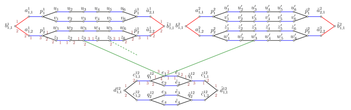
Figure 1: An illustration of construction of graph $G^{\prime}$ in W[1]-hardness of ASM for constant sized preference list. Here, blue colored edges belongs to the stable matching $\mu$. Here, $n=4$, $m=4$, and $r=2$

Claim 1

Graph $G^{\prime}$ is bipartite.

Proof

We show that $G^{\prime}$ is a bipartite graph by creating a bipartition $(X,Y)$ for $G^{\prime}$ as follows. We define the following sets.

$$A=\{a_{j,\ell}^{i}:i\in[k],j\in[\log_{2}(\nicefrac{{n}}{{2}})],\ell\in[\beta_{j}]\}$$

$$\tilde{A}=\{\tilde{a}_{j,\ell}^{i}:i\in[k],j\in[\log_{2}(\nicefrac{{n}}{{2}})],\ell\in[\beta_{j}]\}$$

$$B=\{b_{j,\ell}^{i}:i\in[k],j\in[\log_{2}(\nicefrac{{n}}{{2}})],\ell\in[\gamma_{j}]\}$$

$$\tilde{B}=\{\tilde{b}_{j,\ell}^{i}:i\in[k],j\in[\log_{2}(\nicefrac{{n}}{{2}})],\ell\in[\gamma_{j}]\}$$

We add $A$ to $X$ and $\tilde{A}$ to $Y$. Note that there is no edge between the vertices in $A$ (or $\tilde{A}$). Since no vertex of $B$(or $\tilde{B}$) is adjacent to $\tilde{A}$(or $A$), we add $B$ to $Y$ and $\tilde{B}$ to $X$.

Let $P=\{p_{\ell}^{i}:i\in[k],\ell\in[\beta_{1}]\}$ and $\tilde{P}=\{\tilde{p}_{\ell}^{i}:i\in[k],\ell\in[\beta_{1}]\}$. We add $P$ to $Y$ and $\tilde{P}$ to $X$. We define the following sets of vertices.

$$U_{odd}=\{u_{2h-1}:u\in V_{i},i\in[k],h\in[r+1]\}\text{ and }$$

$$U_{even}=\{u_{2h}:u\in V_{i},i\in[k],h\in[r+1]\}$$

We add $U_{odd}$ to $X$ and $U_{even}$ to $Y$. We define the following sets.

$$E_{1}=\{e:e\in E_{ij},\{i,j\}\subseteq[k]\}\text{ and }$$

$$E_{2}=\{\tilde{e}:e\in E_{ij},\{i,j\}\subseteq[k]\}$$

We add $E_{1}$ to $Y$ and $E_{2}$ to $X$.

We next define the following sets.

$$Q=\{q_{\ell}^{ij}:\{i,j\}\subseteq[k],i<j,\ell\in[\rho_{1}]\}\text{ and }$$

$$\tilde{Q}=\{\tilde{q}_{\ell}^{ij}:\{i,j\}\subseteq[k],i<j,\ell\in[\rho_{1}]\}$$

We add $Q$ to $X$ and $\tilde{Q}$ to $Y$. Again define the the following two sets.

$$C=\{c_{h,\ell}^{ij}:\{i,j\}\subseteq[k],i<j,h\in[\log_{2}(\nicefrac{{m}}{{2}})],\ell\in[\rho_{h}]\}$$

$$\tilde{C}=\{\tilde{c}_{h,\ell}^{ij}:\{i,j\}\subseteq[k],i<j,h\in[\log_{2}(\nicefrac{{m}}{{2}})],\ell\in[\rho_{h}]\}$$

We add $C$ to $Y$ and $\tilde{C}$ to $X$. Finally we define the sets,

$$D=\{d_{h,\ell}^{ij}:\{i,j\}\subseteq[k],i<j,h\in[\log_{2}(\nicefrac{{m}}{{2}})],\ell\in[\tau_{h}]\}$$

$$\tilde{D}=\{\tilde{d}_{h,\ell}^{ij}:\{i,j\}\subseteq[k],i<j,h\in[\log_{2}(\nicefrac{{m}}{{2}})],\ell\in[\tau_{h}]\}$$

We add $D$ to $X$ and $\tilde{D}$ to $Y$. Observe that $X$ and $Y$ are independent sets in $G^{\prime}$. Hence, $G^{\prime}$ is a bipartite graph. Figure 2 illustrates this bipartition of the graph $G^{\prime}$.

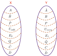
Figure 2: A bipartition of the graph $G^{\prime}$, constructed in the W[1]-hardness of ASM.

This completes the construction of an instance of ASM.

Correctness: Since we are interested in a matching which is at least $t$ more than the size of a stable matching, we need to know the size of a stable matching. Towards this, we construct a stable matching $\mu$ that contains the following set of edge

$$\left(\cup_{\begin{subarray}{c}u\in V(G)\end{subarray}}\{u_{2h-1}u_{2h}\in E(G^{\prime}):h\in[r+1]\}\right)\bigcup\left(\cup_{\begin{subarray}{c}e\in E(G)\end{subarray}}\{e\tilde{e}\in E(G^{\prime})\}\right)$$

Additionally, for each $i\in[k]$ and $\ell\in[\nicefrac{{n}}{{2}}]$, we add $a_{1,\ell}^{i}p_{\ell}^{i}$ and $\tilde{a}_{1,\ell}^{i}\tilde{p}_{\ell}^{i}$ to $\mu$. For each $i\in[k]$, $j\in[\log_{2}(\nicefrac{{n}}{{2}})]\setminus\{1\}$, and $\ell\in[\beta_{j}]$, we add $a_{j,\ell}^{i}b_{j-1,\ell}^{i}$ and $\tilde{a}_{j,\ell}^{i}\tilde{b}_{j-1,\ell}^{i}$ to $\mu$. For each $\{i,j\}\subseteq[k]$, $i<j$, and $\ell\in[\nicefrac{{m}}{{2}}]$, we add $c_{1,\ell}^{ij}q_{\ell}^{ij}$ and $\tilde{c}_{1,\ell}^{ij}\tilde{q}_{\ell}^{ij}$ to $\mu$. For each $\{i,j\}\subseteq[k]$, $i<j$, $h\in[\log_{2}(\nicefrac{{m}}{{2}})]\setminus\{1\}$, and $\ell\in[\rho_{h}]$, we add $c_{h,\ell}^{ij}d_{h-1,\ell}^{ij}$ and $\tilde{c}_{h,\ell}^{ij}\tilde{d}_{(h-1)\ell}^{ij}$ to $\mu$. This completes the construction of the matching $\mu$.

Claim 2

Matching $\mu$ has size $kn(r+1)+\nicefrac{{mk(k-1)}}{{2}}+2k(n-2)+k(k-1)(m-2)$. Furthermore, $\mu$ is a stable matching in $G^{\prime}$.

Proof

Due to Section 3, we know that $\mu$ contains at least $kn(r+1)+\nicefrac{{mk(k-1)}}{{2}}$ edges because $|V_{i}|=n$ for each $i\in[k]$ and $|E_{ij}|=m$ for each $\{i,j\}\subseteq[k]$. The other edges added to $\mu$ can be counted separately, leading to the following relation.

$$|\mu|= ~{}kn(r+1)+\nicefrac{{mk(k-1)}}{{2}}+kn+k(n-4)+(\nicefrac{{mk(k-1)}}{{2}})+(m-4)(\nicefrac{{k(k-1)}}{{2}})$$

$$= ~{}kn(r+1)+\nicefrac{{mk(k-1)}}{{2}}+2k(n-2)+k(k-1)(m-2)$$

Next, to show that $\mu$ is a stable matching in $G^{\prime}$, we will exhaustively argue for each vertex in $G^{\prime}$ that there is no blocking edge incident to it.

We begin by noting that for any vertex $u\in V(G)$, vertices $u_{1}$ and $u_{2}$ in $G^{\prime}$ prefer each other over any other vertex in $G^{\prime}$. Therefore, edge $u_{1}u_{2}$ is a static edge and must belong to every stable matching in $G^{\prime}$. Similarly, for any $e\in E(G)$, we note that $e\tilde{e}$ is a static edge in $G^{\prime}$, and thus belongs to every stable matching in $G^{\prime}$. For any $u\in V(G)$ and $h\in[r]$, we know that vertex $u_{2h+1}$ is the first preference of $u_{2h+2}$. Thus, there cannot exist a blocking edge incident to $u_{2h+2}$, where $h\in[r]$. Moreover, for any $h\in[r]$, the vertices that $u_{2h+1}$ prefers over $u_{2h+2}$ are matched to their top preferences. Consequently, there cannot be a blocking edge incident to $u_{2h+1}$.

Since for each $u\in V_{i}$, $i\in[k]$, vertices $u_{1}$ and $u_{2r+2}$ are matched to their top preferences respectively, thus for any $\ell\in[\nicefrac{{n}}{{2}}]$ the edges $u_{1}p_{\ell}^{i}$ and $u_{2r+2}\tilde{p}_{\ell}^{i}$ cannot be a blocking edge with respect to $\mu$. Thus, there is no blocking edge incident to $p_{\ell}^{i}$ and $\tilde{p}_{\ell}^{i}$, for $\ell\in[\nicefrac{{n}}{{2}}]$. Analogously, we can argue that there is no blocking edge incident on $q_{h}^{ij}$ and $\tilde{q}_{h}^{ij}$, for any $\{i,j\}\subseteq[k]$, $i<j$ and $h\in[\nicefrac{{m}}{{2}}]$.

Since for each $i\in[k]$, $j\in[\log_{2}(\nicefrac{{n}}{{2}})]$, and $\ell\in[\beta_{j}]$, vertices $a_{j,\ell}^{i}$ and $\tilde{a}_{j,\ell}^{i}$ are matched to their top preferences respectively, there is no blocking edge incident to $a_{j,\ell}^{i}$ or $\tilde{a}_{j,\ell}^{i}$. Analogously, there is no blocking edge incident on $c_{h,\ell}^{ij}$ or $\tilde{c}_{h,\ell}^{ij}$, for any $\{i,j\}\subseteq[k],i<j,h\in[\log_{2}(\nicefrac{{m}}{{2}})]$, and $\ell\in[\rho_{h}]$.

For any $i\in[k]$, $j\in[\log_{2}(\nicefrac{{n}}{{2}})]$, and $\ell\in[\gamma_{j}]$, vertices that $b_{j,\ell}^{i}$ prefers over $a_{j+1,\ell}^{i}$ (i.e., $a_{j,2\ell-1}^{i}$ and $a_{j,2\ell}^{i}$) are matched to their top preferences respectively, there is no blocking edge incident to $b_{j,\ell}^{i}$. By symmetry, there is no blocking edge incident to $\tilde{b}_{h,\ell}^{i}$. Analogously, there is also no blocking edge incident to $d_{h^{\prime},\ell^{\prime}}^{ij}$, or $\tilde{d}_{h^{\prime},\ell^{\prime}}^{ij}$, for any $\{i,j\}\subseteq[k],i<j,h^{\prime}\in[\log_{2}(\nicefrac{{m}}{{2}})]$, and $\ell^{\prime}\in[\tau_{h}]$.

Hence, we can conclude that $\mu$ is a stable matching in $G^{\prime}$.

Next, we will formally prove the equivalence between the instance of MCQ and the instance of ASM. In particular, we will prove the following lemma.

Lemma 1

$\mathcal{I}=(G,(V_{1},\ldots,V_{k}))$ is a Yes-instance of MCQ if and only if $\mathcal{J}=(G^{\prime},\mathcal{L},\mu,k^{\prime},t)$ is a Yes-instance of ASM.

Before giving the proof of Lemma 1, we give a structural property of any matching in $G^{\prime}$ which will be used later.

Claim 3

Let $\tilde{\eta}$ be a matching in $G^{\prime}$ of size $|\mu|+t$. Then, $\tilde{\eta}$ is a perfect matching in $G^{\prime}$.

Proof

We first count the number of vertices in $G^{\prime}$. Note that for each vertex in $G$, we have a path of length $2r+2$ in $G^{\prime}$. Since $|V(G)|=nk$, there are $(2r+2)nk$ such vertices in $V(G^{\prime})$. For each $i\in[k]$ and $\ell\in[\nicefrac{{n}}{{2}}]$, we added $p_{\ell}^{i},\tilde{p}_{\ell}^{i}$. Hence, we have added $kn$ special vertices to $V(G^{\prime})$. Note that there are $2k(n-2)$ vertices in the set $\{a_{j\ell}^{i},\tilde{a}_{j\ell}^{i}:i\in[k],j\in[\log_{2}(\nicefrac{{n}}{{2}})],\ell\in[\nicefrac{{n}}{{2^{j}}}]\}$. Additionally, we have $k(n-2)$ vertices in the set $\{b_{j,\ell}^{i},\tilde{b}_{j,\ell}^{i}:i\in[k],j\in[\log_{2}(\nicefrac{{n}}{{2}})],\ell\in[\nicefrac{{n}}{{2^{j+1}}}]\}$.

Now, we count the vertices in $G^{\prime}$ that corresponding to edges in $G$. Note that for each edge in $G$, we have two vertices in $G^{\prime}$. Since $|E_{ij}|=m$, where $\{i,j\}\subseteq[k]$, there are $2m(\nicefrac{{k(k-1)}}{{2}})$ vertices in the set $\{e,\tilde{e}:e\in E(G)\}$. There are $m(\nicefrac{{k(k-1)}}{{2}})$ vertices in the set $\{q_{\ell}^{ij},\tilde{q}_{\ell}^{ij}:\{i,j\}\subseteq[k],i<j,\ell\in[\nicefrac{{m}}{{2}}]\}$. There are $k(k-1)(m-2)$ vertices in the set $\{c_{h,\ell}^{ij},\tilde{c}_{h,\ell}^{ij}:\{i,j\}\subseteq[k],i<j,h\in[\log_{2}(\nicefrac{{m}}{{2}})],\ell\in[\nicefrac{{m}}{{2^{h}}}]\}$. Similarly, we have $\nicefrac{{k(k-1)(m-2)}}{{2}}$ vertices in the set $\{d_{h,\ell}^{ij},\tilde{d}_{h,\ell}^{ij}:\{i,j\}\subseteq[k],h\in[\log_{2}(\nicefrac{{m}}{{2}})],\ell\in[\nicefrac{{m}}{{2^{h+1}}}]\}$. Hence,

$$|V(G^{\prime})|=2(r+1)kn+2k(2n-3)+mk(k-1)+2k(k-1)(m-\nicefrac{{3}}{{2}})$$

Recall that $\lvert\mu\rvert=(r+1)kn+\nicefrac{{mk(k-1)}}{{2}}+2k(n-2)+k(k-1)(m-2)$ and $t=k+\nicefrac{{k(k-1)}}{{2}}$. Therefore, $|\tilde{\eta}|=(r+1)kn+\nicefrac{{mk(k-1)}}{{2}}+k(2n-3)+k(k-1)(m-\nicefrac{{3}}{{2}})$. Hence, $\tilde{\eta}$ is a perfect matching in $G^{\prime}$.

Now, we are ready to prove Lemma 1.

Proof (Proof of Lemma 1)

In the forward direction, let $S$ be a solution of MCQ for $\mathcal{I}$, i.e $|X\cap V_{i}|=1$, for each $i\in[k]$ and $G[X]$ is a clique in $G$.

Defining a solution matching: We construct a solution $\eta$ to $\mathcal{J}$ as follows. Initially, we set $\eta=\mu$. Suppose that $u=S\cap V_{i}$, then from $\eta$ we delete edges $\{u_{2h-1}u_{2h}:h\in[r+1]\}$; and add edges $\{u_{2h}u_{2h+1}:h\in[r]\}$.

Let $\ell=\sigma(V_{i},u)$, i.e the solution $S$ contains the $\ell^{th}$ vertex of the set $V_{i}$. Then, we delete $\{a_{1,\lceil\nicefrac{{\ell}}{{2}}\rceil}^{i}p_{\lceil\nicefrac{{\ell}}{{2}}\rceil}^{i},\tilde{a}_{1,\lceil\nicefrac{{\ell}}{{2}}\rceil}^{i}\tilde{p}_{\lceil\nicefrac{{\ell}}{{2}}\rceil}^{i}\}$ from $\eta$ and add $\{u_{1}p_{\lceil\nicefrac{{\ell}}{{2}}\rceil}^{i},u_{2r+2}\tilde{p}_{\lceil\nicefrac{{\ell}}{{2}}\rceil}^{i}\}$ to $\eta$. Additionally, we delete $\{a_{j,h}^{i}b_{j-1,h}^{i},\tilde{a}_{j,h}^{i}\tilde{b}_{j-1,h}^{i}:j\in[\log_{2}(\nicefrac{{n}}{{2}})]\setminus\{1\},h=\lceil\nicefrac{{\ell}}{{2^{j}}}\rceil\}$ and add set $\{a_{j,h}^{i}b_{j,h^{\prime}}^{i},\tilde{a}_{j,h}^{i}\tilde{b}_{j,h^{\prime}}^{i}:j\in[\log_{2}(\nicefrac{{n}}{{2}})],h=\lceil\nicefrac{{\ell}}{{2^{j}}}\rceil,h^{\prime}=\lceil\nicefrac{{\ell}}{{2^{j+1}}}\rceil\}$ to $\eta$.

Let edge $e=E(G[S])\cap E_{ij}$, i.e. edge $e$ in $E_{ij}$ is in the clique solution, for some $\{i,j\}\subseteq[k]$. Suppose that for some $\ell\in[m]$, $e$ is the $\ell^{th}$ edge in $E_{ij}$. Then, we delete set $\{e\tilde{e},q_{\lceil\nicefrac{{\ell}}{{2}}\rceil}^{ij}c_{1,\lceil\nicefrac{{\ell}}{{2}}\rceil}^{ij},\tilde{q}_{\lceil\nicefrac{{\ell}}{{2}}\rceil}^{ij}\tilde{c}_{1,\lceil\nicefrac{{\ell}}{{2}}\rceil}^{ij}\}$ from $\eta$ and add $\{eq_{\lceil\nicefrac{{\ell}}{{2}}\rceil}^{ij},\tilde{e}\tilde{q}_{\lceil\nicefrac{{\ell}}{{2}}\rceil}^{ij}\}$ to $\eta$. Additionally, we delete edges $\{c_{h,s}^{ij}d_{h-1,s}^{ij},~{}\tilde{c}_{h,s}^{ij}\tilde{d}_{h-1,s}^{ij}:h\in[\log_{2}(\nicefrac{{m}}{{2}})]\setminus\{1\}\},s=\lceil\nicefrac{{\ell}}{{2^{h}}}\rceil\}$ from $\eta$ and add set $\{c_{h,s}^{ij}d_{h,s^{\prime}}^{ij},~{}\tilde{c}_{h,s}^{ij}\tilde{d}_{h,s^{\prime}}^{ij}:h\in[\log_{2}(\nicefrac{{m}}{{2}})],s=\lceil\nicefrac{{\ell}}{{2^{h}}}\rceil,s^{\prime}=\lceil\nicefrac{{\ell}}{{2^{h+1}}}\rceil\}$. Due to the construction of $\eta$, clearly it is a matching.

The following result implies that the matching $\eta$ constructed as above satisfies the size bound of a solution for our instance $\mathcal{J}$ of ASM.

Claim 4

Matching $\eta$ described above has size $|\mu|+k+\nicefrac{{k(k-1)}}{{2}}$.

Proof

For each (clique) vertex $u=S\cap V_{i}$, where $i\in[k]$, we delete $r+2\log_{2}(\nicefrac{{n}}{{2}})+1$ edges from $\eta$ (which also belong to $\mu$), and add $r+2\log_{2}(\nicefrac{{n}}{{2}})+2$ edges to $\eta$. This gives us an an additional $k$ edges in $\eta$.

Similarly, for each clique edge $e=E(G[S])\cap E_{ij}$, where $\{i,j\}\subseteq[k],i<j$, we delete $2\log_{2}(\nicefrac{{m}}{{2}})+1$ edges from $\eta$ (which also belong to $\mu$), and add $2\log_{2}(\nicefrac{{m}}{{2}})+2$ edges to $\eta$. This, gives us an additional $\nicefrac{{k(k-1)}}{{2}}$ edges in $\eta$. Thus, in total $|\eta|=|\mu|+k+\nicefrac{{k(k-1)}}{{2}}$.

Next, we prove that $\eta$ has $k^{\prime}=k+\nicefrac{{k(k-1)}}{{2}}$ blocking edges. Due to Proposition 1, for a blocking edge with respect to $\eta$, at least one of its endpoint is in $V(\mu\triangle\eta)$. Therefore, we only need to investigate the vertices of $V(\mu\triangle\eta)$. We begin by characterizing the vertices in the set $V(\mu\triangle\eta)$.

Note that

$$V(\mu\triangle\eta)=~{}~{}\{u_{2h-1},u_{2h}:u\in S,h\in[r+1]\}\cup\{e,\tilde{e}:e\in E(G[S])\}\\ \hskip 42.67912pt\bigcup\hskip 5.0pt\cup_{i\in[k]}\{p_{\lceil\nicefrac{{\ell}}{{2}}\rceil}^{i},\tilde{p}_{\lceil\nicefrac{{\ell}}{{2}}\rceil}^{i},a_{j,\lceil\nicefrac{{\ell}}{{2^{j}}}\rceil}^{i},\tilde{a}_{j,\lceil\nicefrac{{\ell}}{{2^{j}}}\rceil}^{i},b_{j,\lceil\nicefrac{{\ell}}{{2^{j+1}}}\rceil}^{i},\tilde{b}_{j,\lceil\nicefrac{{\ell}}{{2^{j+1}}}\rceil}^{i}:\\ \hskip 113.81102pt\text{ $S$ contains the $\ell^{th}$ vertex of $V_{i}$ },j\in[\log_{2}(\nicefrac{{n}}{{2}})]\}\\ \hskip 42.67912pt\bigcup\hskip 5.0pt\cup_{\{i,j\}\subseteq[k],i<j}\{q_{\lceil\ell/2\rceil}^{ij},\tilde{q}_{\lceil\ell/2\rceil}^{ij},c_{h,\lceil\ell/2^{h}\rceil}^{ij},\tilde{c}_{h,\lceil\ell/2^{h}\rceil}^{ij},d_{h,\lceil\ell/2^{h+1}\rceil}^{ij},\tilde{d}_{h,\lceil\ell/2^{h+1}\rceil}^{ij}:\\ \hskip 113.81102pt\text{ $G[S]$ contains the $\ell^{th}$ edge of $E_{ij}$, }h\in[\log(m/2)]\}$$

Claim 5

For any $u\in S$ and any $h\in[r]$, there is no blocking edge with respect to $\eta$ that is incident to the vertex $u_{2h+1}$ or $u_{2h+2}$.

Proof

For any value $h\in[r]$, vertex $u_{2h+1}$ is matched to its most preferred vertex in $\eta$, namely $u_{2h}$. Therefore, there is no blocking edge incident on $u_{2h+1}$. For any $h^{\prime}\in[r-1]$, we have $N(u_{2h^{\prime}+2})=\langle u_{2h^{\prime}+1},u_{2h^{\prime}+3}\rangle$. Thus, there is no blocking edge incident to $u_{2h^{\prime}+2}$.

Suppose that $u$ is the $\ell^{th}$ vertex in $V_{i}$. Then, we have $N(u_{2r+2})=\langle u_{2r+1},\tilde{p}_{\lceil\nicefrac{{\ell}}{{2}}\rceil}^{i}\rangle$, and we know that the edge $u_{2r+2}\tilde{p}_{\lceil\nicefrac{{\ell}}{{2}}\rceil}^{i}$ is in $\eta$. However, since $u_{2r+1}$ is matched to its most preferred neighbor, it follows that there is no blocking edge incident to $u_{2r+2}$.

Claim 6

For any vertex $u\in S$, $u_{1}u_{2}$ is a blocking edge in $G^{\prime}$ with respect to $\eta$. Moreover, there is no other blocking edge incident to $u_{1}$ or $u_{2}$ in $G^{\prime}$

Proof

Since vertices $u_{1}$ and $u_{2}$ in $G^{\prime}$ prefer each other over any other vertex, and the edge $u_{1}u_{2}$ is not in $\eta$, it must be a blocking edge with respect to $\eta$.

Let $\ell=\sigma(V_{i},u)$, i.e the solution $S$ contains the $\ell^{th}$ vertex of the set $V_{i}$. Then, $N(u_{1})=\langle u_{2},p_{\lceil\nicefrac{{\ell}}{{2}}\rceil}^{i}\rangle$, and we know that $u_{1}p_{\lceil\nicefrac{{\ell}}{{2}}\rceil}^{i}\in\eta$. Thus, other than $u_{1}$ $u_{2}$, there is no other blocking edge incident to $u_{1}$ in $\eta$. Similarly, since $N(u_{2})=\langle u_{1},u_{3}\rangle$, and $u_{2}u_{3}\in\eta$, it follows that there is no other blocking edge incident to $u_{2}$.

Claim 7

For any $i\in[k]$ and $\ell\in[\nicefrac{{n}}{{2}}]$, there is no blocking edge with respect to $\eta$ that is incident to vertex $p_{\ell}^{i}$ or $\tilde{p}_{\ell}^{i}$.

Proof

Let $u=V_{i}(2\ell-1)$ and $v=V_{i}(2\ell)$, i.e, $u$ and $v$ denote the $2\ell-1^{st}$ and $2\ell^{th}$ elements of $V_{i}$, respectively.

Suppose that $\{u,v\}\cap S=\emptyset$. Then, due to the construction of $\eta$, we know that $u_{1}u_{2}$ and $v_{1}v_{2}$ are in $\eta$. Recall that $N(p_{\ell}^{i})=\langle u_{1},v_{1},a_{1\ell}^{i}\rangle$. Since $u_{1}$ and $v_{1}$ are matched to their most preferred neighbor in $\eta$, namely $u_{2}$ and $v_{2}$, so there is no blocking edge incident to $p_{\ell}^{i}$. Hence, this case is resolved.

Suppose that $u\in S$. Then, $p_{\ell}^{i}u_{1}\in\eta$. Since $p_{\ell}^{i}$ prefers $u_{1}$ over any other vertex, so there is no blocking edge incident to $p_{\ell}^{i}$.

Suppose that $v\in S$. Then, $p_{\ell}^{i}v_{1}\in\eta$, by the construction of $\eta$. Since $|S\cap V_{i}|=1$, and $v\in S$, it follows that $u\notin S$. Hence, $u_{1}u_{2}\in\eta$, implying that $u_{1}$ is matched to its most preferred neighbor $u_{2}$. Therefore, there is no blocking edge with respect to $\eta$ that is incident to $p_{\ell}^{i}$. By symmetry, we can argue that there is no blocking edge incident to $\tilde{p}_{\ell}^{i}$.

Claim 8

For any $i\in[k],j\in[\log_{2}(\nicefrac{{n}}{{2}})]$ and $\ell\in[\beta_{j}]$, there is no blocking edge with respect to $\eta$ that is incident to vertex $a_{j,\ell}^{i}$ or $\tilde{a}_{j,\ell}^{i}$.

Proof

We first consider the case when $j=1$. Recall that $N(a_{1,\ell}^{i})=\langle p_{\ell}^{i},b_{1,\ell}^{i}\rangle$. If $a_{1,\ell}^{i}p_{\ell}^{i}\in\eta$, then $a_{1,\ell}^{i}$ is matched to its most preferred vertex. Thus, there is no blocking edge incident on $a_{1,\ell}^{i}$. Suppose that $a_{1,\ell}^{i}b_{1,\ell}^{i}\in\eta$. In this case, by the construction of $\eta$, either $p_{\ell}^{i}u_{1}\in\eta$ or $p_{\ell}^{i}v_{1}\in\eta$, where $u=V_{i}(2\ell-1)$ and $v=V_{i}(2\ell)$. Note that $p_{\ell}^{i}$ prefers both $u_{1}$ and $v_{1}$ over $a_{1,\ell}^{i}$. Hence, there is no blocking edge incident to $a_{1,\ell}^{i}$. Next, we consider the case when $j\geq 2$. Recall that $N(a_{j,\ell}^{i})=\langle b_{j-1,\ell}^{i},b_{j,\ell}^{i}\rangle$. If $a_{j,\ell}^{i}b_{j-1,\ell}^{i}\in\eta$, then $a_{j,\ell}^{i}$ is matched to its most preferred vertex. Thus, there is no blocking edge incident on $a_{j\ell}^{i}$. Suppose that $a_{j,\ell}^{i}b_{j,\ell}^{i}\in\eta$. Since $a_{j,\ell}^{i}$ is the last preference of $b_{j-1,\ell}^{i}$ (and $b_{j-1,\ell}^{i}$ is matched to $a_{j-1,\ell}^{i}$ in $\eta$), we can conclude that there is no blocking edge incident to $a_{j,\ell}^{i}$. Similarly, there is no blocking edge with respect to $\eta$ that is incident to $\tilde{a}_{j,\ell}^{i}$

Claim 9

For any $i\in[k],j\in[\log_{2}(\nicefrac{{n}}{{2}})]$, and $\ell\in[\gamma_{j}]$, there is no blocking edge with respect to $\eta$ that is incident to vertex $b_{j\ell}^{i}$ or $\tilde{b}_{j\ell}^{i}$.

Proof

We first consider the case when $j\in[\log_{2}(\nicefrac{{n}}{{2}})-1]$. Recall that
$N(b_{j,\ell}^{i})=\langle a_{j,2\ell-1}^{i},~{}a_{j,2\ell}^{i},~{}a_{j+1,\ell}^{i}\rangle$. If $b_{j,\ell}^{i}a_{j,2\ell-1}^{i}\in\eta$, then $b_{j,\ell}^{i}$ is matched to its most preferred vertex. Hence, there is no blocking edge incident on $b_{j,\ell}^{i}$. Suppose that $b_{j,\ell}^{i}a_{j,2\ell}^{i}\in\eta$. Note that $a_{j,2\ell-1}^{i}$ is the only vertex that $b_{j,\ell}^{i}$ prefers over $a_{j,2\ell}^{i}$. Since $b_{j,\ell}^{i}$ is the last preference of $a_{j,2\ell-1}^{i}$, and $a_{j,2\ell-1}^{i}$ is saturated in $\eta$ (Claims 3 and 4 imply that $\eta$ is a perfect matching), there is no blocking edge incident on $b_{j,\ell}^{i}$. If $b_{j,\ell}^{i}a_{j+1,\ell}^{i}\in\eta$, then using the same argument as earlier, there is no blocking edge incident on $b_{j,\ell}^{i}$. Now, consider the case when $j=\log_{2}(\nicefrac{{n}}{{2}})$. Since $N(b_{j,1}^{i})=\langle a_{j,1}^{i},a_{j,2}^{i}\rangle$, there is no blocking edge incident on $b_{j,1}^{i}$ using the same arguments as earlier. Similarly, there is no blocking edge incident on $\tilde{b}_{j,\ell}^{i}$ with respect to $\eta$.

Claim 10

For any $\{i,j\}\subseteq[k],i<j$, and $\ell\in[\nicefrac{{m}}{{2}}]$, there is no blocking edge with respect to $\eta$ that is incident to vertex $q_{\ell}^{ij}$ or $\tilde{q}_{\ell}^{ij}$.

Proof

The proof is similar to the proof of Claim 7.

Claim 11

For any $\{i,j\}\subseteq[k],i<j$, $h\in[\log_{2}(\nicefrac{{m}}{{2}})]$ and $\ell\in[\rho_{h}]$, there is no blocking edge with respect to $\eta$ that is incident to vertex $c_{h,\ell}^{ij}$ or $\tilde{c}_{h,\ell}^{ij}$.

Proof

The proof is similar to the proof of Claim 8.

Claim 12

For any $\{i,j\}\subseteq[k],i<j,h\in[\log_{2}(\nicefrac{{m}}{{2}})],\ell\in[\tau_{h}]$, there is no blocking edge with respect to $\eta$ that is incident to vertex $d_{h,\ell}^{ij}$ or $\tilde{d}_{h,\ell}^{ij}$.

Proof

The proof is similar to the proof of Claim 9.

Claim 13

Let $e$ denote an edge in the clique $G[S]$. Then, the edge $e\tilde{e}$ in $G^{\prime}$ is a blocking edge with respect to $\eta$. Moreover, there is no other blocking edge with respect to $\eta$ that is incident to vertex $e$ or $\tilde{e}$ in $G^{\prime}$.

Proof

Since vertices $e$ and $\tilde{e}$ prefer each other over any other vertex in $G^{\prime}$, and the edge $e\tilde{e}$ is not in $\eta$, it must be a blocking edge with respect to $\eta$.

Let $e=uv$, that is vertices $u\in V_{i}$ and $v\in V_{j}$ are the two endpoints of the edge $e$ in $G$. Suppose that for some $h,h^{\prime}\in[r]$, we have $h=\sigma(E_{u},e)$ and $h^{\prime}=\sigma(E_{v},e)$ i.e, $e$ is the $h^{th}$ element of $E_{u}$ and the $h^{\prime th}$ element of $E_{v}$.

Recall that $N_{G^{\prime}}(e)=\langle\tilde{e},u_{2h+1},v_{2h^{\prime}+1},q_{\lceil\nicefrac{{\ell}}{{2}}\rceil}^{ij}\rangle$, where $\ell=\sigma(E_{ij},e)$, i.e, $e$ is the $\ell^{th}$ element in the set $E_{ij}$. By the construction of $\eta$, we know that the edge $eq_{\lceil\nicefrac{{\ell}}{{2}}\rceil}^{ij}$ is in $\eta$. Moreover, since $\{u,v\}\subseteq S$, we know that vertices $u_{2h+1}$ and $v_{2h^{\prime}+1}$ are matched to their most preferred vertices in $\eta$. Hence, $e\tilde{e}$ must be the only blocking edge with respect to $\eta$ that is incident to $e$. Similarly, we note that since $N(\tilde{e})=\langle e,\tilde{q}_{\lceil\nicefrac{{\ell}}{{2}}\rceil}^{ij}\rangle$ and edge $\tilde{e}\tilde{q}_{\lceil\nicefrac{{\ell}}{{2}}\rceil}^{ij}$ is in $\eta$, the only blocking edge that is incident to the vertex $\tilde{e}$ is $e\tilde{e}$. Thus, the claim is proved.

Note that Claims 5 and 6 imply that for each vertex $u\in S$, there is a unique blocking edge with respect to $\eta$ (namely $u_{1}u_{2}$); and Claim 13 implies that for each edge $e$ in $G[S]$, there is a unique blocking edge (namely $e\tilde{e}$ )with respect to $\eta$. Moreover, Claims 7–12 imply that there are no other blocking edges with respect to $\eta$. Hence, in total there are $k^{\prime}=k+\nicefrac{{k(k-1)}}{{2}}$ blocking edges with respect to $\eta$. Thus, we can conclude that the forward direction is proved $(\Rightarrow$).

$(\Leftarrow)$ In the reverse direction, let $\eta$ be a matching of size at least $\lvert\mu\rvert+k+\nicefrac{{k(k-1)}}{{2}}$ such that $\eta$ has at most $k+\nicefrac{{k(k-1)}}{{2}}$ blocking edges. Due to the size of $\eta$, we can infer that it is a perfect matching.

Let ${\mathtt{B}}_{\eta}$ be the set of blocking edges with respect to $\eta$. We first note some properties of matching $\eta$ and the set ${\mathtt{B}}_{\eta}$. We start by identifying the edges in ${\mathtt{B}}_{\eta}$.

Note that in our instance, the static edges in $G^{\prime}$ are of the following type: For any $u\in V(G)$, edge $u_{1}u_{2}$ in $G^{\prime}$ is a static edge and is called the u-type static edge; for any $e\in E(G)$, edge $e\tilde{e}$ in $G^{\prime}$ is a static edge and is called the e-type static edge.

In the following claims, we prove that a blocking edge with respect to $\eta$ is either a u-type static edge or e-type static edge. In fact, for each $i\in[k]$, there is unique u-type static edge which is a blocking edge, and for each $\{i,j\}\subseteq[k]$, there is unique e-type static edge which is a blocking edge.

Claim 14 (u-type static edge)

For each $i\in[k]$, there exists $u\in V_{i}$, such that $u_{1}u_{2}$ is a blocking edge with respect to $\eta$.

Proof

Since $\eta$ is a perfect matching, for each $i\in[k]$ and $j=\log_{2}(\nicefrac{{n}}{{2}})$, vertex $b_{j,1}^{i}$ is saturated by $\eta$. Recall that $N(b_{j,1}^{i})=\langle a_{j,1}^{i},a_{j,2}^{i}\rangle$. Therefore, there exists a (unique) $z\in[2]$, such that $b_{j,1}^{i}a_{j,z}^{i}\in\eta$.

Since $\eta$ is a perfect matching and $b_{j-1,z}^{i}$ has two other neighbors $a_{j-1,2z-1}^{i}$ and $a_{j-1,2z}^{i}$, it follows that either $b_{j-1,z}^{i}a_{j-1,2z-1}^{i}\in\eta$ or $b_{j-1,z}^{i}a_{j-1,2z}^{i}\in\eta$. We view the index $j$ as indicating a level, the highest being $\log_{2}(\nicefrac{{n}}{{2}})$. As we go down each level starting from the highest, we obtain a matching edge in $\eta$. The lowest level is reached when for some value $h\in[\nicefrac{{n}}{{4}}]$, we reach the vertex $b_{1,h}^{i}$. For this vertex, there are two possible matching partners in $\eta$: $a_{1,2h-1}^{i}$ or $a_{1,2h}^{i}$. Thus, for some value $h^{\prime}\in\{2h-1,2h\}$, edge $b_{1,h}^{i}a_{1,h^{\prime}}^{i}\in\eta$.

Since $\eta$ is a perfect matching, $p_{h^{\prime}}^{i}$ must be matched to either $x_{1}$ or $y_{1}$ (its other two neighbors) in $\eta$, where $x=V_{i}(2h^{\prime}-1)$ and $y=V_{i}(2h^{\prime})$ i.e, $x$ is the $2h^{\prime}-1^{st}$ element of $V_{i}$ and $y$ is the $2h^{\prime th}$ element of $V_{i}$. If $p_{h^{\prime}}^{i}x_{1}\in\eta$, then since $x_{1}$ and $x_{2}$ are each others first preference, the edge $x_{1}x_{2}\in{\mathtt{B}}_{\eta}$. Otherwise, if $p_{h^{\prime}}^{i}y_{1}\in\eta$, then with analogous argument, it follows that the edge $y_{1}y_{2}\in{\mathtt{B}}_{\eta}$. Hence, the result is proved.

Claim 15 (e-type static edge)

For each $\{i,j\}\subseteq[k]$, there exists $e\in E_{ij}$, such that $e\tilde{e}$ is a blocking edge with respect to $\eta$ and $q_{\lceil\nicefrac{{\ell}}{{2}}\rceil}^{ij}e\in\eta$, where $e$ is the $\ell^{th}$ element of $E_{ij}$.

Proof

Since $\eta$ is a perfect matching, for each $\{i,j\}\subseteq[k]$ and $h=\log_{2}(\nicefrac{{m}}{{2}})$, the vertex $d_{h,1}^{ij}$ must be saturated by $\eta$. Recall that $N(d_{h,1}^{ij})=\langle c_{h,1}^{ij},c_{h,2}^{ij}\rangle$. Therefore, there exists a (unique) $z\in[2]$, such that $d_{h,1}^{ij}c_{h,z}^{ij}\in\eta$.

Now, since $\eta$ is a perfect matching, and $N(d_{h-1,z}^{ij})=\langle c_{h-1,2z-1}^{ij},c_{h-1,2z}^{ij},c_{h,z}^{ij}\rangle$, either $d_{h-1,z}^{ij}c_{h-1,2z-1}^{ij}\in\eta$ or $d_{h-1,z}^{ij}c_{h-1,2z}^{ij}\in\eta$. We view the index $h$ as indicating a level, the highest being $\log_{2}(\nicefrac{{m}}{{2}})$. As we go down each level starting from the highest, we obtain a matching edge in $\eta$. The lowest level is reached when for some value $h^{\prime}\in[\nicefrac{{m}}{{4}}]$, we reach the vertex $d_{1,h^{\prime}}^{ij}$. For this vertex, there are two possible matching partners in $\eta$: $c_{1,2h^{\prime}-1}^{ij}$ or $c_{1,2h^{\prime}}^{ij}$. Thus, for some $\bar{h}\in\{2h^{\prime}-1,2h^{\prime}\}$, edge $d_{1,h^{\prime}}^{ij}c_{1,\bar{h}}^{ij}\in\eta$.

Since $\eta$ is a perfect matching, $q_{\bar{h}}^{ij}$ is matched to either $e$ or $e^{\prime}$ in $\eta$, where $e=E_{ij}(2\bar{h}-1)$ and $e^{\prime}=E_{ij}(2\bar{h})$, i.e, $e$ is the $2\bar{h}-1^{st}$ element of $E_{ij}$ and $e^{\prime}$ is the $2\bar{h}^{th}$ element of $E_{ij}$. If $q_{\bar{h}}^{ij}e\in\eta$, then since $e$ and $\tilde{e}$ are each others first preference, edge $e\tilde{e}\in{\mathtt{B}}_{\eta}$. Else if $q_{\bar{h}}^{ij}e^{\prime}\in\eta$, then with analogous argument, it follows that $e^{\prime}\tilde{e^{\prime}}\in{\mathtt{B}}_{\eta}$. Hence, the result is proved.

Corollary 1

For each $i\in[k]$, there exists a unique $u\in V_{i}$, such that the edge $u_{1}u_{2}$ is a blocking edge with respect to $\eta$; and for each $\{i,j\}\subseteq[k]$, there exists a unique $e\in E_{ij}$, such that $e\tilde{e}$ is a blocking edge with respect to $\eta$.

Proof

Using Claims  14 and  15, we know that there are at least $k+\nicefrac{{k(k-1)}}{{2}}$ blocking edges with respect to $\eta$. Since $k^{\prime}=k+\nicefrac{{k(k-1)}}{{2}}$, the uniqueness condition follows.

Conversely, we can also argue the following.

Corollary 2

Any blocking edge with respect to $\eta$ is either a $u$-type static edge or an $e$-type static edge.

Proof

Using Corollary 1, we know that there are at least $k$ u-type blocking edges and $\nicefrac{{k(k-1)}}{{2}}$ $e$-type blocking edges with respect to $\eta$. Since $k^{\prime}=k+\nicefrac{{k(k-1)}}{{2}}$, there cannot exist any other (besides $u$-type and $e$-type) blocking edge with respect to $\eta$.

Next, we prove that the $e$-type (static) blocking edges force certain edges to be in the matching $\eta$.

Claim 16

For any $\{i,j\}\subseteq[k]$, consider some $e\in E_{ij}$ such that $e\tilde{e}$ is a blocking edge with respect to $\eta$. Then, for the value $\ell=\sigma(E_{ij},e)$, the edge $q_{\lceil\nicefrac{{\ell}}{{2}}\rceil}^{ij}e$ is in $\eta$.

Proof

By Claim 15, there exists an edge $e^{\prime}\in E_{ij}$ such that $e^{\prime}\tilde{e^{\prime}}$ is a blocking edge with respect to $\eta$ and $q_{\lceil\nicefrac{{\ell^{\prime}}}{{2}}\rceil}^{ij}e^{\prime}$ is in $\eta$, where $\ell^{\prime}=\sigma(E_{ij},e^{\prime})$. By Corollary 1, we know that $e^{\prime}=e$.

Claim 17 (consistency between u-type static edge and e-type static edge)

Suppose that for some $\{i,j\}\subseteq[k],i<j$, we have $e\in E_{ij}$ such that $e\tilde{e}$ is a blocking edge with respect to $\eta$. Let $u$ and $v$ denote the two endpoints of the edge $e$ in $G$. Then, both $u_{1}u_{2}$ and $v_{1}v_{2}$ are blocking edges with respect to $\eta$.

Proof

For the sake of contradiction, suppose that both $u_{1}u_{2}$ and $v_{1}v_{2}$ are not blocking edges with respect to $\eta$. Without loss of generality, we may assume that $u_{1}u_{2}$ is not a blocking edge. Since $u_{1}$ and $u_{2}$ prefer each other over any other vertex, $u_{1}u_{2}\in\eta$, otherwise it will contradict the fact that $u_{1}u_{2}$ is not a blocking edge. For any $h\in[r]$, suppose that $u_{2h+1}e^{\prime}\in\eta$, where $e^{\prime}=\sigma(E_{u},h)$. Since $e^{\prime}$ and $\tilde{e^{\prime}}$ prefer each other over any other vertex $e^{\prime}\tilde{e^{\prime}}\in\mathtt{B}_{\eta}$. Since $u_{2h+1}e^{\prime}\in\eta$, the edge $q_{\lceil\nicefrac{{\ell}}{{2}}\rceil}^{ij}e^{\prime}\notin\eta$, where $\ell=\sigma(E_{ij},e^{\prime})$, a contradiction to Claim 16. Thus, for any $h\in[r]$, $u_{2h+1}e^{\prime}\notin\eta$, where $e^{\prime}=\sigma(E_{u},h)$. Since $u_{1}u_{2}\in\eta$ and $\eta$ is a perfect matching, we can infer that for each $h\in[r]$, $u_{2h+1}u_{2h+2}\in\eta$. Since $e\tilde{e}\in\mathtt{B}_{\eta}$, due to Claim 16, $q_{\lceil\nicefrac{{\ell}}{{2}}\rceil}^{ij}e\in\eta$, where $\ell=\sigma(E_{ij},e)$. Note that there exists $h\in[r]$ such that $u_{2h+1}e\in E(G^{\prime})$. Since $u_{2h+1}$ prefers $e$ more than its matched partner in $\eta$, i.e., $u_{2h+2}$, and $e$ prefers $u_{2h+1}$ more than its matched partner in $\eta$, $u_{2h+1}e\in\mathtt{B}_{\eta}$, a contradiction to Corollary 2.

Next, we construct two sets $S$ and $E_{S}$ as follows. Let $S=\{u\in V(G):u_{1}u_{2}\in{\mathtt{B}}_{\eta}\}$, i.e, the set of vertices in $G$ that correspond to a $u$-type static blocking edge. Let $E_{S}=\{e\in E(G):e\tilde{e}\in{\mathtt{B}}_{\eta}\}$, i.e, the set of edges in $G$ that correspond to a $e$-type static blocking edge.

We claim that $G_{S}=(S,E_{S})$ is a clique, and $|S\cap V_{i}|=1$, for each $i\in[k]$. Using Claim 17, we know that for each edge $e\in E_{S}$, we have $\{u,v\}\subseteq S$, where $u$ and $v$ are the two endpoints of the edge $e$.

Moreover, using Corollary 1, we that $|V_{i}\cap S|=1$ for each $i\in[k]$ and $|E_{S}|=\nicefrac{{k(k-1)}}{{2}}$. Hence, we may conclude that $G_{S}$ is a clique on $k$ vertices. This completes the proof of the lemma.

Thus, Theorem 1.1 is proved.

4 W$[1]$-hardness of LS-ASM

In this section, we show the parameterized intractability of LS-ASM with respect to several parameters. In particular, we prove Theorem 1.2 and Theorem 1.3.

4.1 Proof of Theorem 1.2

We again give a polynomial-time parameter preserving many-to-one reduction from MCQ on regular graphs. Let $(G,k)$ be an instance of MCQ. To construct an instance $(G^{\prime},\mathcal{L},\mu,k^{\prime},q,t)$ of LS-ASM, we construct a graph $G^{\prime}$, a set of $\mathcal{L}$ containing the preference list of each vertex of $G^{\prime}$, and a stable matching $\mu$ as defined in the proof of Theorem 1.1. We set the parameters $k^{\prime}$ and $t$ also as in the proof of Theorem 1. We set parameter $q$ as follows:

$$q=(2r+3)k+\frac{3k(k-1)}{2}+4k\log_{2}\Big{(}\frac{n}{2}\Big{)}+2k(k-1)\log_{2}\Big{(}\frac{m}{2}\Big{)}$$

Next, we show that $(G,k)$ is a Yes-instance of MCQ if and only if $(G^{\prime},\langle,\rangle\mu,k^{\prime},q,t)$ is a Yes-instance of LS-ASM. In the forward direction, let $X$ be a solution of MCQ for $(G,k)$. We construct a matching $\eta$ as defined in the above proof. As proved above, $|\eta|=|\mu|+t$ and the number of blocking edges with respect to $\eta$ is $k^{\prime}$. Now, we show that $|\mu\triangle\eta|\leq q$. Recall that for each vertex in $X$, we delete $r+2\log_{2}(\nicefrac{{n}}{{2}})+1$ edges from $\eta$ (which also belongs to $\mu$), and add $r+2\log_{2}(\nicefrac{{n}}{{2}})+2$ edges to $\eta$. Similarly, for each edge in $E(G[X])$, we delete $2(\log_{2}\nicefrac{{m}}{{2}})+1$ edge from $\eta$ which is also in $\mu$, and add $2(\log_{2}\nicefrac{{m}}{{2}})+2$ edges to $\eta$. Hence,

$$|\mu\triangle\eta|=(2r+3)k+\frac{3k(k-1)}{2}+4k\log_{2}\Big{(}\frac{n}{2}\Big{)}+2k(k-1)\log_{2}\Big{(}\frac{m}{2}\Big{)}$$

This completes the proof in the forward direction. The proof of backward direction is same as the proof of the backward direction of Theorem 1.1.

4.2 Proof of Theorem 1.3

We again give a polynomial-time parameter preserving many-to-one reduction from MCQ similar to the one in Theorem 1.1. Here, we do not need graph to be a regular graph.

Construction. Given an instance $\mathcal{I}=(G,(V_{1},\ldots,V_{k}))$ of MCQ, we construct an instance $\mathcal{J}=(G^{\prime},\mathcal{L},\mu,k^{\prime},q,t)$ of LS-ASM as follows. For any $\{i,j\}\subseteq[k]$, such that $i<j$, we use $E_{ij}$ to denote the set of edges between sets $V_{i}$ and $V_{j}$.

• For each vertex $v\in V(G)$, we add four vertices in $G^{\prime}$, denoted by $\{u_{i}:i\in[4]\}$, connected via a path: $(u_{1},u_{2},u_{3},u_{4})$ in $G^{\prime}$.

• For each edge $e\in E_{ij}$, we add vertices $e$ and $\tilde{e}$ to $V(G^{\prime})$, and the edge $e\tilde{e}$ to $E(G^{\prime})$.

• For each $i\in[k]$, we add two vertices $p_{1}^{i},p_{2}^{i}$, and for each $\{i,j\}\subseteq[k]$ where $i<j$, we add two vertices $q_{1}^{ij},q_{2}^{ij}$ to $V(G^{\prime})$.

• For each $i\in[k]$ and for each vertex $u\in V_{i}$, we add two edges $u_{1}p_{1}^{i}$ and $u_{4}p_{2}^{i}$ to $E(G^{\prime})$. For each $\{i,j\}\subseteq[k]$, $i<j$, and for each edge $e\in E_{ij}$, we add four edges $q_{1}^{ij}e,q_{2}^{ij}\tilde{e},eu_{3}$, and $ev_{3}$ to $E(G^{\prime})$.

Figure 3 describes the construction of $G^{\prime}$. Note that $V(G^{\prime})=4\lvert V(G)\rvert+2\lvert E(G)\rvert+2k+k(k-1)$. Recall that in the construction of an instance in the proof of Theorem 1.1, for each vertex in $V(G)$, we added a path of length $2r+2$, while here we add a path of length $4$. Moreover, instead of adding $n$ vertices $p_{\ell}^{i}$ and $\tilde{p}_{\ell}^{i}$, for each $i\in[k]$, $\ell\in[\nicefrac{{n}}{{2}}]$, we only add two vertices $p_{1}^{i}$ and $p_{2}^{i}$. Similarly, we added only two vertices $q_{1}^{ij}$ and $q_{2}^{ij}$ instead of adding $m$ such vertices. Furthermore, here we did not add the other special vertices which we added in the previous reduction. This is how we decrease the length of augmenting paths. But, note that degree of vertices $u_{3}$, $p_{1}^{i},p_{2}^{i},q_{1}^{ij},q_{2}^{ij}$, where $u\in V_{i}$, $\{i,j\}\subseteq[k],i<j$, is large.

For any vertex $u\in V(G)$, we define

$$\mathscr{E}_{u}=\{e\in V(G^{\prime})\colon e\in E(G)\text{ and }u\text{ is an endpoint of }e\}$$

The preference list of each vertex in $G^{\prime}$ is presented in Table 2.

Matching $\mu$: Let $\mu=\{u_{1}u_{2},u_{3}u_{4},e\tilde{e}\colon u\in V(G),e\in E(G),\text{ and }i\in[k]\}$. Clearly, $\mu$ is a matching. Note that $\lvert\mu\rvert=2\lvert V(G)\rvert+\lvert E(G)\rvert$.

Parameter: We set $k^{\prime}=k+\nicefrac{{k(k-1)}}{{2}}$, $q=5k+\nicefrac{{3k(k-1)}}{{2}}$, and $t=k^{\prime}$.

Clearly, this construction can be carried out in polynomial time. Next, we will prove some structural properties about our construction, namely that the graph $G^{\prime}$ is bipartite (Claim 18) and $\mu$ is a stable matching (Claim 19).

Claim 18

Graph $G^{\prime}$ is bipartite.

Proof

We show that $G^{\prime}$ is a bipartite graph by creating a bipartition for $G^{\prime}$ as follows. For each $i\in[k]$, and each $u\in V_{i}$, we assign $p_{1}^{i}$, $u_{2}$ and $u_{4}$ to one part and $p_{2}^{i}$, $u_{1}$ and $u_{3}$ to another part. For each $\{i,j\}\subseteq[k]$, $i<j$, since a vertex $e\in V(G^{\prime})$ (corresponding to the edge $e=uv,u\in V_{i},v\in V_{j}$) is connected to $u_{3}$ and $v_{3}$, we assign $e$ and $q_{2}^{ij}$ to the part containing $p_{1}^{i}$, and assign $\tilde{e}$ and $q_{1}^{ij}$ to the part containing $p_{2}^{i}$. Observe that each part is an independent set. Hence $G^{\prime}$ is a bipartite graph.

Claim 19

$\mu$ is a stable matching.

Proof

We begin by noting that for any vertex $u\in V(G)$, vertices $u_{1}$ and $u_{2}$ prefer each other over any other vertex in $G^{\prime}$. Therefore, edge $u_{1}u_{2}$ is a static edge and must belong to every stable matching in $G^{\prime}$. Similarly, for each $e\in E(G)$, we note that $e\tilde{e}$ is a static edge in $G^{\prime}$, and thus belongs to every stable matching in $G^{\prime}$. Since $u_{3}$ is the first preference of $u_{4}$, and the vertices which $u_{3}$ prefers over $u_{4}$ ( i.e., $u_{2}$ and vertices in $\mathscr{E}_{u}$) are matched to their first preferred vertices, it follows that there is no blocking edge with respect to $\mu$. Hence, $\mu$ is a stable matching in $G^{\prime}$.

For each $i\in[k]$ and each $u\in V_{i}$, we have the following preference lists:

$u_{1}\colon$	$\langle u_{2},p_{1}^{i}\rangle$
$u_{2}\colon$	$\langle u_{1},u_{3}\rangle$
$u_{3}\colon$	$\langle u_{2},[\mathscr{E}_{u}],u_{4}\rangle$
$u_{4}\colon$	$\langle u_{3},p_{2}^{i}\rangle$

For each edge $e\in E_{ij}$ with endpoints $u\in V_{i}$ and $v\in V_{j}$ , where $\{i,j\}\subseteq[k]$, $i<j$, we have the following preference lists:

$e\colon$	$\langle\tilde{e},u_{3},v_{3},q_{1}^{ij}\rangle$
$\tilde{e}\colon$	$\langle e,q_{2}^{ij}\rangle$

For each $i\in[k]$ and $\{i,j\}\subseteq[k]$, $i<j$, we have the following preference lists for the remaining vertices:

$p_{1}^{i}\colon$	$\langle[N(p_{1}^{i})]\rangle$
$p_{2}^{i}\colon$	$\langle[N(p_{2}^{i})]\rangle$
$q_{1}^{ij}\colon$	$\langle[N(q_{1}^{ij})]\rangle$
$q_{2}^{ij}\colon$	$\langle[N(q_{2}^{ij})]\rangle$

Table 2: Preference lists in the constructed instance of W[1]-hardness of LS-ASM when parameterized by $k+q+t$. Here, for a set $S$, the symbol $[S]$ denotes that the vertices in this set are listed in some arbitrarily strict order and the notation $\langle\cdot,\cdot\rangle$ denotes the order of preference over neighbors.

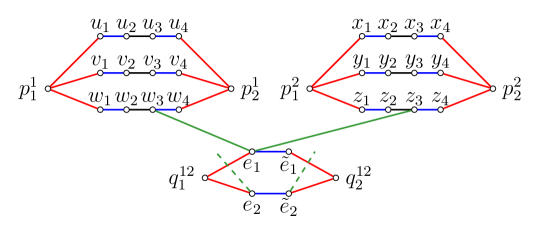
Figure 3: An illustration of the construction of graph $G^{\prime}$ in W[1]-hardness of LS-ASM. Here, blue colored edges belongs to the stable matching $\mu$. Note that $V_{1}=\{u,v,w\}$ and $V_{2}=\{x,y,z\}$, and $e_{1}$ and $e_{2}$ are edges in $E_{12}$.

Correctness. Next, we show the equivalence between the instance $\mathcal{I}$ of MCQ and $\mathcal{J}$ of LS-ASM. Formally, we prove the following:

Lemma 2

$\mathcal{I}=(G,(V_{1},\ldots,V_{k}))$ is a Yes-instance of MCQ if and only if $\mathcal{J}=(G^{\prime},\mathcal{L},\mu,k^{\prime},q,t)$ is a Yes-instance of LS-ASM.

Proof

In the forward direction, let $X$ be a solution of MCQ for $\mathcal{I}$, i.e., for each $i\in[k]$, $|X\cap V_{i}|=1$, and $G[X]$ is a clique. We construct a solution $\eta$ to $\mathcal{J}$ as follows. Initially, we set $\eta=\mu$. For each $i\in[k]$, if $u\in X\cap V_{i}$, we delete edges $u_{1}u_{2}$ and $u_{3}u_{4}$ from $\eta$, and add edges $u_{1}p_{1}^{i},u_{2}u_{3}$, and $u_{4}p_{2}^{i}$ to $\eta$. Also, for each $\{i,j\}\subseteq[k]$, $i<j$, if $e\in E(G[X])\cap E_{ij}$, then we remove the edge $e\tilde{e}$ from $\eta$ and add edges $eq_{1}^{ij}$ and $\tilde{e}q_{2}^{ij}$ to $\eta$.

Claim 20

$\eta$ is a matching

Proof

For each $i\in[k]$ and $u\in X\cap V_{i}$, edges $u_{1}p_{1}^{i}$, $u_{2}u_{3}$, and $u_{4}p_{2}^{i}$ are in $\eta$, and no other edge incident to $u_{1},u_{2},u_{3}$ or $u_{4}$ is in $\eta$. Since for each $i\in[k]$, $|X\cap V_{i}|=1$, there is only one edge incident to each $p_{1}^{i}$ and $p_{2}^{i}$. Similarly, for each $e\in E(G[X])$, there is only one matching edge incident to $e$ and $\tilde{e}$, namely $eq_{1}^{ij}$ and $\tilde{e}q_{2}^{ij}$. Since, the remaning edges of $\eta$ are the same as in $\mu$, this implies $\eta$ is a matching.

Claim 21

$|\eta|=|\mu|+t$ and $|\mu\triangle\eta|=q$

Proof

Note that for each $u\in X$, we delete two edges from $\eta$ (which also belongs to $\mu$), and add three edges to $\eta$. Similarly, for an edge $e\in E(G[X])$, we delete one edge from $\eta$ which is also in $\mu$, and add two edges to $\eta$. Hence, $|\eta|=|\mu|+k+\nicefrac{{k(k-1)}}{{2}}=|\mu|+t$, and $|\mu\triangle\eta|=5k+\nicefrac{{3k(k-1)}}{{2}}=q$.

Next, we prove that $\eta$ has $k^{\prime}=k+\nicefrac{{k(k-1)}}{{2}}$ blocking edges. Due to Proposition  1, to count the blocking edges with respect to $\eta$, we only investigate the vertices of $V(\mu\triangle\eta)$. Note that

$$V(\mu\triangle\eta)={} \{u_{j},p_{\ell}^{i}\in V(G^{\prime})\colon u\in X\cap V_{i},j\in[4],\ell\in[2],i\in[k]\}$$

$$\bigcup\quad\{e,\tilde{e},q_{\ell}^{ij}\in V(G^{\prime})\colon e\in E(G[X]),\{i,j\}\subseteq[k],i<j,\ell\in[2]\}$$

Claim 22

Let $u\in X$. There is no blocking edge incident to $u_{3}$ or $u_{4}$ with respect to $\eta$.

Proof

Since $u_{2}u_{3}\in\eta$, and $u_{3}$ prefers $u_{2}$ over any other vertex, there is no blocking edge incident to $u_{3}$. Let $u\in V_{i}$, for some $i\in[k]$. Recall that the preference list of $u_{4}$ is $\langle u_{3},p_{2}^{i}\rangle$. Since there is no blocking edge incident to $u_{3}$ and $u_{4}p_{2}^{i}\in\eta$, it follows that there is no blocking edge incident to $u_{4}$.

Claim 23

Let $u\in X$. Then, $u_{1}u_{2}$ is a blocking edge with respect to $\eta$. Moreover, there is no other blocking edge incident to $u_{1}$ or $u_{2}$.

Proof

Since $u_{1}$ and $u_{2}$ prefer each other over any other vertex and $u_{1}u_{2}\notin\eta$, it is a blocking edge with respect to $\eta$. Let $u\in V_{i}$, for some $i\in[k]$. Since the preference list of $u_{1}$ is $\langle u_{2},p_{1}^{i}\rangle$ and $u_{1}p_{1}^{i}\in\eta$, there is no other blocking edge incident to $u_{1}$. Similarly, since the preference list of $u_{2}$ is $\langle u_{1},u_{3}\rangle$ and $u_{2}u_{3}\in\eta$, it follows that there is no other blocking edge incident to $u_{2}$.

Using Claims 22 and 23, for each $i\in[k]$ and $u\in X\cap V_{i}$, we introduce exactly one blocking edge with respect to $\eta$ by deleting $u_{1}u_{2}$ and $u_{3}u_{4}$ from $\eta$, and adding edges $u_{1}p_{1}^{i},u_{2}u_{3}$, and $u_{4}p_{2}^{i}$ to it. Since $|X|=k$, in total we introduce $k$ blocking edges with respect to $\eta$ due to the said alternation.

Claim 24

For each $i\in[k]$, there is no blocking edge incident to $p_{1}^{i}$ or $p_{2}^{i}$ with respect to $\eta$.

Proof

Let $u\in X\cap V_{i}$. Then, by the construction of $\eta$, $u_{4}p_{2}^{i}\in\eta$. Let $v\in V_{i}\setminus\{u\}$. Since $|X\cap V_{i}|=1$, $v\notin X$. Hence, $v_{4}v_{3}\in\eta$. Since $v_{4}$ prefers $v_{3}$ over $p_{2}^{i}$, $v_{4}p_{2}^{i}$ is not a blocking edge. Hence, there is no blocking edge incident to $p_{2}^{i}$ as $N(p_{2}^{i})=\{w_{4}\colon w\in V_{i}\}$. Similarly, there is no blocking edge incident to $p_{1}^{i}$.

Claim 25

Let $e\in E(G[X])$. Then, $e\tilde{e}$ is a blocking edge with respect to $\eta$. Moreover, there is no other blocking edge incident to $e$ or $\tilde{e}$.

Proof

Since $e\tilde{e}\notin\eta$, and $e$ and $\tilde{e}$ prefer each other over any other vertex, $e\tilde{e}$ is a blocking edge with respect to $\eta$. Let $e=uv$ where $u\in V_{i}$, and $v\in V_{j}$. Recall that the preference list of $e$ is $\langle\tilde{e},u_{3},v_{3},q_{1}^{ij}\rangle$. Since $u_{3}$ does not prefer $e$ over $u_{2}(=\eta(u_{3}))$, $u_{3}e$ is not a blocking edge with respect to $\eta$. Similarly, $v_{3}e$ is not a blocking edge with respect to $\eta$. Since $eq_{1}^{ij}\in\eta$, $e\tilde{e}$ is the only blocking edge incident to $e$ for $\eta$. Since $N(\tilde{e})=\{e,q_{2}^{ij}\}$, and $\tilde{e}q_{2}^{ij}\in\eta$, there is no other blocking edge incident to $\tilde{e}$ with respect to $\eta$.

Claim 26

For each $\{i,j\}\subseteq[k],i<j$, there is no blocking edge incident to $q_{1}^{ij}$ or $q_{2}^{ij}$ with respect to $\eta$.

Proof

Let $e_{1}\in E(G[X])\cap E_{ij}$. Hence, by the construction of $\eta$, ${e_{1}}q_{1}^{ij},\tilde{e_{1}}q_{2}^{ij}\in\eta$. Let $e_{2}\in E_{ij}\setminus\{e_{1}\}$. Since $|E(G[X])\cap E_{ij}|=1$, $e_{2}$ does not belong to $E(G[X])$. Therefore, by the construction of $\eta$, ${e_{2}}\tilde{e_{2}}\in\eta$. Since ${e_{2}}$ and $\tilde{e_{2}}$ prefer each other over any other vertex, there is no blocking edge incident to ${e_{2}}$ or $\tilde{e_{2}}$. Hence, ${e_{2}}q_{1}^{ij}$ and $\tilde{e_{1}}q_{2}^{ij}$ are not blocking edges. Since $N(q_{1}^{ij})=\{e\in V(G^{\prime})\colon e\in E_{ij}\}$, and $N(q_{2}^{ij})=\{\tilde{e}\in V(G^{\prime})\colon e\in E_{ij}\}$, there is no blocking edge incident to $q_{1}^{ij}$ or $q_{2}^{ij}$.

Hence, for each $e\in E(G[X])$, we introduce one blocking edge $e\tilde{e}$ with respect to $\eta$. That is, we introduce $\nicefrac{{k(k-1)}}{{2}}$ blocking edges. Using Claims 22 to 26, there are $k+\nicefrac{{k(k-1)}}{{2}}$ blocking edges for $\eta$. This completes the proof in the forward direction.

In the reverse direction, let $\eta$ be a matching of size at least $|\mu|+t$ such that $|\mu\triangle\eta|\leq 5k+\nicefrac{{3k(k-1)}}{{2}}$, and $\eta$ has at most $k^{\prime}$ blocking edges. Recall that $|V(G^{\prime})|=4\lvert V(G)\rvert+2\lvert E(G)\rvert+2k+k(k-1)$, $\mu=2\lvert V(G)\rvert+\lvert E(G)\rvert$, and $t=k+\nicefrac{{k(k-1)}}{{2}}$. Hence, $\eta$ is a perfect matching in $G^{\prime}$.

Note that, similar to Theorem 1.1, in our instance, the static edges in $G^{\prime}$ are of the following type: For any $u\in V(G)$, edge $u_{1}u_{2}$ in $G^{\prime}$ is a static edge and is called the $u$-type static edge; for any $e\in E(G)$, edge $e\tilde{e}$ in $G^{\prime}$ is a static edge and is called the $e$-type static edge.

Let ${\mathtt{B}}_{\eta}$ be the set of blocking edges with respect to $\eta$. Let us note the following properties of the set ${\mathtt{B}}_{\eta}$. Specifically we show that an edge in ${\mathtt{B}}_{\eta}$ is either a $u$-type static edge or an $e$-type static edge. In fact, for each $i\in[k]$, there is a unique $u$-type static edge which is a blocking edge, and for each $\{i,j\}\subseteq[k]$, there is a unique $e$-type static edge in ${\mathtt{B}}_{\eta}$.

Claim 27 ($u$-type static edge)

For each $i\in[k]$, there exists a vertex $u\in V_{i}$ such that the edge $u_{1}u_{2}\in{\mathtt{B}}_{\eta}$.

Proof

Since $\eta$ is a perfect matching, $p_{1}^{i}$ is saturated by $\eta$, for each $i\in[k]$. Since $N(p_{1}^{i})=\{u_{1}\colon u\in V_{i}\}$, we have that $p_{1}^{i}u_{1}\in\eta$, for some $u\in V_{i}$. Since $u_{1}$ and $u_{2}$ prefer each other over any other vertex, it follows that $u_{1}u_{2}\in{\mathtt{B}}_{\eta}$.

Claim 28 ($e$-type static edge)

For each $\{i,j\}\subseteq[k]$, there exists an edge $e\in E_{ij}$ such that the edge $e\tilde{e}\in{\mathtt{B}}_{\eta}$.

Proof

Since $\eta$ is a perfect matching, $q_{1}^{ij}$ is saturated by $\eta$, for each $\{i,j\}\subseteq[k]$, where $i<j$. Since $N(q_{1}^{ij})=\{e\in V(G^{\prime})\colon e\in E_{ij}\}$, $eq_{1}^{ij}\in\eta$, for some $e\in V(G^{\prime})$. Since $e$ and $\tilde{e}$ prefer each other over any other vertex, it follows that $e\tilde{e}\in{\mathtt{B}}_{\eta}$.

Using Claims  27 and  28, and the fact that $|{\mathtt{B}}_{\eta}|=k+\nicefrac{{k(k-1)}}{{2}}$, we have following two properties of ${\mathtt{B}}_{\eta}$.

Corollary 3

For each $i\in[k]$, there exists a unique vertex $u\in V_{i}$ such that the edge $u_{1}u_{2}\in{\mathtt{B}}_{\eta}$; and for each $\{i,j\}\subseteq[k]$ where $i<j$, there exists a unique edge $e\in E_{ij}$ such that the edge $e\tilde{e}\in{\mathtt{B}}_{\eta}$.

Corollary 4

Any edge in the set ${\mathtt{B}}_{\eta}$ is either a $u$-type static edge or an $e$-type static edge.

Next, we note a property that forces an edges in the matching $\eta$.

Claim 29

For any $\{i,j\}\subseteq[k]$, consider some $e\in E_{ij}$ such that $e\tilde{e}\in{\mathtt{B}}_{\eta}$. Then $q_{1}^{ij}e\in\eta$.

Proof

Suppose $q_{1}^{ij}e\notin\eta$, then since $\eta$ is a perfect matching, there exists a vertex $e^{\prime}\in V(G^{\prime})$ such that $q_{1}^{ij}e^{\prime}\in\eta$. Since $e^{\prime}$ and $\tilde{e^{\prime}}$ prefer each other over any other vertex, $e^{\prime}\tilde{e^{\prime}}\in{\mathtt{B}}_{\eta}$. Recall that $N(q_{1}^{ij})=\{e^{\prime}\in V(G^{\prime})\colon e^{\prime}\in E_{ij}\}$. Therefore, $e^{\prime}\in E_{ij}$, a contradiction to the uniqueness criteria in Corollary 3. Therefore, $q_{1}^{ij}e\in\eta$.

Claim 30

Let $e=uv$, $u\in V_{i}$ and $v\in V_{j}$ where $\{i,j\}\subseteq[k]$ and $i<j$. If $e\tilde{e}\in{\mathtt{B}}_{\eta}$, then $\{u_{1}u_{2},v_{1}v_{2}\}\subseteq{\mathtt{B}}_{\eta}$,

Proof

We first show that $u_{1}u_{2}\in{\mathtt{B}}_{\eta}$. Recall that the preference list of $u_{3}$ is $\langle u_{2},[\mathscr{E}_{u}],u_{4}\rangle$. If $\eta(u_{3})=u_{2}$, then since $u_{1}$ and $u_{2}$ prefer each other over any other vertex, $u_{1}u_{2}\in{\mathtt{B}}_{\eta}$.

Suppose that $\eta(u_{3})=e^{\prime}$ where $e^{\prime}\in\mathscr{E}_{u}$, then since $e^{\prime}$ and $\tilde{e^{\prime}}$ prefer each other over any other vertex, $e^{\prime}\tilde{e^{\prime}}\in{\mathtt{B}}_{\eta}$. Since $u_{3}e^{\prime}\in\eta$, we get a contradiction to Claim 29. Therefore, $\eta(u_{3})\notin\mathscr{E}_{u}$. Since $\eta$ is a perfect matching, $\eta(u_{3})=u_{4}$. Note that $u_{3}$ prefers the vertex $e$ over $u_{4}$. Since, $e\tilde{e}\in{\mathtt{B}}_{\eta}$, by Claim  29 we have that $q_{1}^{ij}e\in\eta$. Note that $e$ also prefers $u_{3}$ over $q_{1}^{ij}$. Therefore, $u_{3}e\in{\mathtt{B}}_{\eta}$. This contradicts Corollary 4. Similarly, we can show that $v_{1}v_{2}\in{\mathtt{B}}_{\eta}$.

Next, we construct two sets $S$ and $E_{S}$ as follows. Let $S=\{u\in V(G)\colon u_{1}u_{2}\in{\mathtt{B}}_{\eta},i\in[k]\}$, and $E_{S}=\{e\in E(G)\colon e\tilde{e}\in{\mathtt{B}}_{\eta},\{i,j\}\subseteq[k]\}$. We claim that $G_{S}=(S,E_{S})$ is a clique, and $|S\cap V_{i}|=1$, where $i\in[k]$. Let $e=uv$, where $u\in V_{i}$, and $v\in V_{j}$. Using Claim 30, for each $e\tilde{e}\in{\mathtt{B}}_{\eta}$, $\{u_{1}u_{2},v_{1}v_{2}\}\subseteq{\mathtt{B}}_{\eta}$. Hence for each $uv\in E_{S}$, $\{u,v\}\subseteq S$. Using Corollary 3, $|S\cap V_{i}|=1$, i.e., $|S|=k$, and $|E_{S}|=\nicefrac{{k(k-1)}}{{2}}$. Hence, $G_{S}$ is a clique. This completes the proof.

5 FPT Algorithm for LS-ASM

In this section, we give FPT algorithm for LS-ASM with respect to $q+d$ (Theorem 1.4). Recall that $d$ is the degree of the graph $G$, and $q$ is the symmetric difference between a solution matching and the given stable matching $\mu$. Suppose $\eta$ is a hypothetical solution to $(G,\mathcal{L},\mu,k,q,t)$. Let matchings $\mu=\mu_{1}\uplus\mu_{2}$ and $\eta=\mu_{2}\uplus\eta_{2}$. Observe that we can obtain $\eta$ from $\mu$, by deleting $\mu_{2}$, and adding the edges in $\eta_{2}$. Equivalently, we can find $\eta$, if we know $\mu\triangle\eta$, as $\mu\triangle\eta=\mu_{2}\uplus\eta_{2}$. Thus, our goal is reduced to find $\mu\triangle\eta$. Now, we begin with the description of our algorithm, which has three phases: Vertex Separation, Edge Separation, and Size-Fitting. An example describes the algorithm in Figure 4. We begin with the description of a randomized algorithm which will be derandomized later using $n$-$p$-$q$-lopsided universal family [13]. Given an instance $(G,\mathcal{L},\mu,k,q,t)$ of LS-ASM, we proceed as follows.

Phase I: Vertex Separation

Then, the following properties hold for $G$ that is colored using the function $f$:

• Every vertex in $V(\mu\triangle\eta)$ is colored $1$ with probability at least $\frac{1}{2^{2q}}$.

• Let $B$ be a set of the neighbors of the vertices in $V(\mu\triangle\eta)$ outside the set $V(\mu\triangle\eta)$, that is, $B=N_{G}(V(\mu\triangle\eta))$, and $D$ be the set of matching partners of the vertices in $B$, in the matching $\mu$, if they exist. Every vertex in $B\cup D$ is colored $2$ with probability at least $\frac{1}{2^{4qd}}$. To see this note that $|\mu\triangle\eta|\leq q$ and the maximum degree of a vertex in the graph $G$ is $d$, and so $|B\cup D|\leq 2|B|=2|N_{G}(V(\mu\triangle\eta))|\leq 4qd$.

For $i\in[2]$, let $V_{i}$ denote the set of vertices of the graph $G$, that are colored $i$ using the function $f$. Summarizing the above mentioned properties we get the following.

Lemma 3

Let $V_{1},V_{2}$, $B$ and $D$ be as defined above. Then, with probability at least $\frac{1}{2^{2q+4qd}}$, $V(\mu\triangle\eta)\subseteq V_{1}$ and $B\cup D\subseteq V_{2}$.

Due to Lemma 3, we have the following:

Corollary 5

Every component in $G[V(\mu\triangle\eta)]$ is also a component in $G[V_{1}]$ with probability at least $\frac{1}{2^{2q+4qd}}$.

The proof of Corollary 5 follows from the fact that $V(\mu\triangle\eta)\subseteq V_{1}$ and $B=N_{G}(V(\mu\triangle\eta))$ is a subset of $V_{2}$. Thus, due to Corollary 5, if there exists a component in $C$ containing a vertex $u\in V(G)$ such that $\mu(u)\notin C$, then $C$ is not a component in $G[V(\mu\triangle\eta)]$. Thus, we get the following reduction rule.

Reduction Rule 1

If there exists a component in $C$ containing a vertex $u\in V(G)$ such that $\mu(u)\notin C$, then delete the component $C$ from $G[V_{1}]$.

In light of Corollary 5, to find $\mu\triangle\eta$, in Phase II, we color the edges of $G[V_{1}]$ in order to identify the components of the graph that only contains edges of $\mu\triangle\eta$.

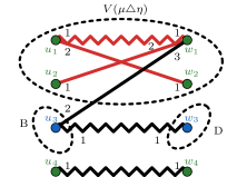
Figure 4: The zigzag edges represent the edges of the stable matching $\mu$. The matching $\eta=\{u_{1}w_{2},u_{2}w_{1},u_{3}w_{3},u_{4}w_{4}\}$, and sets $B$ and $D$ are as defined in the Phase I of the algorithm. Vertex colors $1$ and $2$ in Phase I are represented by green and blue, respectively. Hence, $G_{1}=G[\{u_{1},u_{2},u_{4},w_{1},w_{2},w_{4}\}]$. The red edges represent the edges in $\mu\triangle\eta$ in Phase II.

Phase II: Edge Separation

Let $G_{1}=G[V_{1}]$ and let $G^{\prime}=G_{1}[V(\mu\triangle\eta)]$. Then, the following properties hold for the graph $G_{1}$ that is colored using the function $g$:

• Every edge in $\mu\triangle\eta$ is colored $1$ with probability at least $\frac{1}{2^{q}}$.

• Every edge in $E(G^{\prime})\setminus\!(\mu\triangle\eta)$ is colored $2$ with probability at least $\frac{1}{2^{2qd}}$, because $|V(\mu\triangle\eta)|\leq 2q$ and $d$ is the maximum degree of a vertex in the graph $G$, so $|E(G^{\prime})|\leq 2qd$.

For $i\in[2]$, let $E_{i}$ denote the set of edges of the graph $G_{1}$ that are colored $i$ using the function $g$. Then, due to the above mentioned coloring properties of the graph $G_{1}$, we have the following result:

Lemma 4

Let $G^{\prime}$, $E_{1}$, and $E_{2}$ be as defined above. Then, with probability at least $\frac{1}{2^{q+2qd}}$, $\mu\triangle\eta\subseteq E_{1}$ and $E(G^{\prime})\setminus\!(\mu\triangle\eta)\subseteq E_{2}$.

Note that the edges in $\mu\triangle\eta$ form $\mu$-alternating paths/cycles. Therefore, if there exists a component $C$ in $G_{1}$ such that the set of colored $1$ edges in $C$ do not form a $\mu$-alternating path or a cycle, then we could delete this component from $G_{1}$.

Reduction Rule 2

If there exists a component in $C$ containing a vertex $u\in V(G)$ such that $\mu(u)\notin C$, then delete the component $C$ from $G[V_{1}]$.

Let $G^{\star}=(V_{1},E_{1})$ be a graph on which Reduction Rule 2 is not applicable. Then, we get the following.

Observation 1

Every component in $G^{\star}$ is a $\mu$-alternating path/cycle

The next lemma ensures that we have highlighted our solution with good probability. The proof of it follows from Lemmas 3 and 4.

Lemma 5

Let $(G,\mathcal{L},\mu,k,q,t)$ be a Yes-instance of LS-ASM. Then with probability at least $\frac{1}{2^{3q+6qd}}$, there exists a solution $\eta$ such that (a) it contains every edge of $\mu$ whose both the endpoints are colored $2$ by $f$, and (b) there exists a family of components $\mathscr{C}$ of $G^{\star}$ such that $\eta$ contains all the edges in $\mathscr{C}$ that do not belong to $\mu$ but are colored $1$ by $g$.

In light of Lemma 5, our goal is reduced to find a family of components $\mathscr{C}$ of $G_{1}$ that contains the edges of $\mu\triangle\eta$. Due to Observation 1, to obtain a matching of size $|\mu|+t$, we can choose $t$ components of $G^{\star}$ which are $\mu$-augmenting paths (an alternating path, a path that alternates between matching and a non-matching edge, where the first and the last edge are non-matching edge). However, choosing $t$ components arbitrarily might lead to a large number of blocking edges in the matching $\eta$. Thus, to choose the components of $G^{\star}$ appropriately, we move to Phase III.

Phase III: Size-Fitting with respect to $g$. In this phase, we proceed with the function $g$ and the graph $G^{\star}$ obtained after Phase II (that is the one where every component satisfies the property that edges which are colored $1$ form a $\mu$-alternating path/cycle). Next, we will reduce the instance to an instance of Two-Dimensional Knapsack (2D-KP), and after that use an algorithm for 2D-KP, described in Proposition 2, as a subroutine.

Two-Dimensional Knapsack (2D-KP) Input: A set of tuples, $\mathcal{X}=\{(a_{i},b_{i},p_{i})\in\mathbb{N}^{3}:i\in[n]\}$, and non-negative integers $c_{1},c_{2}$ and $p$ Question: Does there exist a set $Z\subseteq[n]$ such that $\sum_{i\in Z}a_{i}\leq c_{1}$, $\sum_{i\in Z}b_{i}\leq c_{2}$, and $\sum_{i\in Z}p_{i}\geq p$?

Proposition 2

[17] There exists an algorithm $\mathcal{A}$ that given an instance $(\mathcal{X},c_{1},c_{2},p)$ of 2D-KP, in time ${\mathcal{O}}(nc_{1}c_{2})$, outputs a solution if it is a Yes-instance of 2D-KP; otherwise $\mathcal{A}$ outputs “no”.

Next, we construct an instance of 2D-KP as follows. Let $C_{1},\ldots,C_{\ell}$ be the components of the graph $G^{\star}$. For each $i\in[\ell]$, we compute the number of blocking edges, $k_{i}$, incident on the vertices in $C_{i}$ by constructing a matching $\eta_{i}$ as follows. We first add all the edges inside the component $C_{i}$ which are not in $\mu$, to $\eta_{i}$. Further, we add all the edges in $\mu$ which are not in $C_{i}$ and whose at least one of the endpoint is a neighbor of a vertex in $C_{i}$. Clearly, $\eta_{i}$ is a matching in the graph $G$. We set $k_{i}$ as the number of blocking edges with respect to $\eta_{i}$. Let $q_{i}$ denote the number of edges in $C_{i}$, where $i\in[\ell]$. Let $\mu_{i}\subseteq\mu$ be the set edges in $C_{i}$, where $i\in[\ell]$. For each $i\in[\ell]$, let $t_{i}=q_{i}-2|\mu_{i}|$. Intuitively, $t_{i}$ denote the increase in the size of the matching, if we include the $\mu$-alternating path/cycle in $C_{i}$ to the solution matching $\eta$

Let $\mathcal{X}=\{(k_{i},q_{i},t_{i}):i\in[\ell]\}$. This gives us an instance $(\mathcal{X},k,q,t)$ of 2D-KP. We invoke algorithm $\mathcal{A}$ given in Proposition 2 on the instance $(\mathcal{X},k,q,t)$ of 2D-KP. If $\mathcal{A}$ returns a set $Z$, then we return “yes”. Otherwise, we report failure of the algorithm. It is relatively straightforward to create the solution $\eta$ when the answer is “yes”.

Lemma 6

Let $(G,\mathcal{L},\mu,k,q,t)$ be a Yes-instance of LS-ASM. Then, with probability at least $\frac{1}{2^{3q+6qd}}$, we return “yes”.

Proof

Let $\eta$ be a solution claimed in the statement of Lemma 5. Let $\mathscr{C}$ be the family of components mentioned in the statement of Lemma 5. Recall that $C_{1},\ldots,C_{\ell}$ are the components of the graph $G^{\star}$. We next show that $S=\{i\in[\ell]\colon C_{i}\in\mathscr{C}\}$ is a solution to $(\mathcal{X},k,q,t)$. Due to property (b) of the solution $\eta$ and the construction of the instance $(\chi,k,q,t)$, $\sum_{C_{i}\in\mathscr{C}}q_{i}\leq q$ and $\sum_{C_{i}\in\mathscr{C}}t_{i}\geq t$. We next show that $\sum_{C_{i}\in\mathscr{C}}k_{i}\leq k$. Consider a component $C_{i}$ in $\mathscr{C}$. We first recall that if $C_{i}$ is a component in $G[V(\mu\triangle\eta)]$, then $N(V(C_{i}))$ and matching partners of the vertices in $N(V(C_{i}))$, in the matching $\mu$ are colored $2$ by $f$ with probability at least $\frac{1}{2^{4qd}}$. Thus, $\eta_{i}\subseteq\eta$, by the construction of $\eta_{i}$. We next show that every blocking edge with respect to $\eta_{i}$, where $C_{i}$ is a component in $\mathscr{C}$, is also a blocking edge with respect to $\eta$. Let $uv$ be a blocking edge in $\eta_{i}$. Then, $v\succ_{u}\eta_{i}(u)$ and $u\succ_{v}\eta_{i}(v)$. Since $\eta_{i}\subseteq\eta$, it follows that $v\succ_{u}\eta(u)$ and $u\succ_{v}\eta(v)$. Hence, $uv$ is also a blocking edge with respect to $\eta$. Since $k_{i}$ is the the number of blocking edges with respect to $\eta_{i}$, we can infer that $\sum_{C_{i}\in\mathscr{C}}k_{i}\leq k$. Hence, $(\mathcal{X},k,q,t)$ is a Yes-instance of 2D-KP. Therefore, due to Proposition 2, we return “yes”.

Lemma 7

Suppose that $(\chi,k,q,t)$ is a Yes-instance of 2D-KP. Then, $(G,\mathcal{L},\mu,k,q,t)$ is a Yes-instance of LS-ASM.

Proof

Suppose that the algorithm $\mathcal{A}$ in Proposition 2 returns the set $Z$. Given the set $Z$, we obtain the matching $\eta$ as follows. Let $Z(\mathscr{C})$ denote the family of components of $G^{\star}$ corresponding to the indices in $Z$. Formally, $Z(\mathscr{C})=\{C_{i}\colon i\in Z\text{ and }C_{i}\text{ is a component of }G^{\star}\}$. For each component $C\in Z(\mathscr{C})$, we add all the edges in $C$ that are not in $\mu$, to $\eta$. Additionally, we add all the edges in $\mu$ to $\eta$, whose both the endpoints are outside the components in $Z(\mathscr{C})$. We next prove that $\eta$ is a solution to $(G,\mathcal{L},\mu,k,q,t)$.

Claim 31

$\eta$ is a matching.

Proof

Towards the contradiction, suppose that $uv,uw\in\eta$, that is, there exists a pair of edges in $\eta$ that shares an endpoint. Note that $uv$ and $uw$ cannot be in two different components of $G^{\star}$ by the construction of the graph $G^{\star}$. If $uv$ and $uw$ both are in the same component $C\in Z(\mathscr{C})$, then it contradicts Observation 1 as $C$ is also a component in $G^{\star}$. Suppose that $uv\in\mu$ but not in any component in $G^{\star}$. We claim that there is no component in $G^{\star}$ containing $uw$. Towards the contradiction, let $C$ be a component in $G^{\star}$ that contains $uw$. Clearly, $C$ is also a component in $G[V_{1}]$. This contradicts the fact that in Phase I, we have deleted the component $C$ as it contains a vertex $u\in V(G)$ such that $\mu(u)\notin C$. Since $uw\in\eta$ but $uw$ is not in any component in $G^{\star}$, it follows that $uw\in\mu$, by the construction of $\eta$. Since $uv,uw\in\mu$, it contradicts the fact that $\mu$ is a matching.

Claim 32

$|\eta|\geq|\mu|+t$ and $|\mu\triangle\eta|\leq q$.

Proof

For each $C_{i}\in Z(\mathscr{C})$, let $\mu_{i}=\mu\cap E(C_{i})$, that is, $\mu_{i}$ is the set of edges in $C_{i}$ that are in $\mu$. Let $\tilde{\mu}$ be the set of edges in $\mu$ that does not belong to any component in $Z(\mathscr{C})$. Thus, $\mu=\uplus_{C_{i}\in Z(\mathscr{C})}\mu_{i}\uplus\tilde{\mu}$. We first show that if $uv\in\tilde{\mu}$, then both $u$ and $v$ do not belong to any component in $Z(\mathscr{C})$, because if $u$ or $v$ belong to a component $C$ in $Z(\mathscr{C})$, then as argued above it contradicts the fact that we have deleted $C$ in Phase I. Thus, by the construction of $\eta$, $\tilde{\mu}\subseteq\eta$. Furthermore, $\eta=\uplus_{C_{i}\in Z(\mathscr{C})}(E(C_{i})\setminus\mu_{i})\uplus\tilde{\mu}$. Since every $C_{i}\in Z(\mathscr{C})$ is a $\mu$-alternating path due to Observation 1, we have that $|\mu\triangle\eta|=\sum_{C_{i}\in Z(\mathscr{C})}q_{i}\leq q$ as $Z$ is a solution to $(\chi,k,q,t)$. Furthermore, $|\eta|=|\tilde{\mu}|+\sum_{C_{i}\in Z(\mathscr{C})}(E(C_{i})\setminus\mu_{i})=|\tilde{\mu}|+\sum_{C_{i}\in Z(\mathscr{C})}(q_{i}-|\mu_{i}|)=|\tilde{\mu}|+\sum_{C_{i}\in Z(\mathscr{C})}(t_{i}+|\mu_{i}|)$. Since $\sum_{i\in Z}t_{i}\geq t$, we obtained that $|\eta|\geq|\mu|+t$.

Claim 33

There are at most $k$ blocking edges with respect to $\eta$.

Proof

For a component $C_{i}$ in $G^{\star}$, recall the definition of $\eta_{i}$ in Phase III. $\eta_{i}$ contains all the edges in $C_{i}$ which are not in $\mu$ and also the edges which are in $\mu$ but not in $C_{i}$ and whose at least one of the endpoint is a neighbor of a vertex in $C_{i}$. We first prove that every blocking edge with respect to the matching $\eta$ is also a blocking edge with respect to matching $\eta_{i}$, for some $C_{i}\in Z(\mathscr{C})$. Let $uv$ be a blocking edge with respect to $\eta$. Due to Proposition 1 and by the construction of $\eta$, either $u$ or $v$ belongs to a component in $Z(\mathscr{C})$. Without loss of generality, let $u$ belongs to a component $C_{i}\in Z(\mathscr{C})$. Thus, $\eta(u)=\eta_{i}(u)$, by the construction of $\eta$ and $\eta_{i}$. If $v$ is also in $C_{i}$, then $\eta(v)=\eta_{i}(v)$, and hence $uv$ is a blocking edge with respect to $\eta_{i}$. Suppose that $v\notin C_{i}$. Since $uv\in E(G)$, by the construction of the graph $G_{1}$, $v$ does not belong to any other component of $G_{1}$. Thus, by the construction of $\eta$ and $\eta_{i}$, $\eta(v)=\mu(v)$ and $\eta_{i}(v)=\mu(v)$. Therefore, $uv$ is also a blocking edge with respect to $\eta_{i}$. Recall that $k_{i}$ is the number of blocking edges with respect to $\eta_{i}$. Therefore, the number of blocking edges with respect to $\eta$ is at most $\sum_{i\in Z}k_{i}\leq k$.

Due to Claims 31, 32, and 33, we can infer that $\eta$ is a solution to $(G,\mathcal{L},\mu,k,q,t)$.

Due to Lemmas 6 and 7, we obtain a polynomial-time randomized algorithm for LS-ASM which succeeds with probability $\frac{1}{2^{3q+6qd}}$. Therefore, by repeating the algorithm independently $2^{3q+6dq}(\log n)^{{\mathcal{O}}(1)}$ times, where $n$ is the number of vertices in the graph, we obtain the following result:

Theorem 5.1

There exists a randomized algorithm that given an instance of LS-ASM runs in $2^{3q+6dq}n^{{\mathcal{O}}(1)}$ time, where $n$ is the number of vertices in the given graph, and either reports a failure or outputs “yes”. Moreover, if the algorithm is given a Yes-instance of the problem, then it returns “yes” with a constant probability.

5.1 Deterministic FPT algorithm

To make our algorithm deterministic we first introduce the notion of an $n$-$p$-$q$-lopsided universal family. Given a universe $U$ and an integer $\ell$, we denote all the $\ell$-sized subsets of $U$ by ${U\choose\ell}$. We say that a family $\mathcal{F}$ of sets over a universe $U$ with $|U|=n$, is an $n$-$p$-$q$-lopsided universal family if for every $A\in{U\choose p}$ and $B\in{U\setminus A\choose q}$, there is an $F\in\mathcal{F}$ such that $A\subseteq F$ and $B\cap F=\emptyset$.

Lemma 8 ([13])

There is an algorithm that given $n,p,q\in{\mathbb{N}}$ constructs an $n$-$p$-$q$-lopsided universal family $\mathcal{F}$ of cardinality ${p+q\choose p}\cdot 2^{o(p+q)}\log n$ in time $|\mathcal{F}|n$.

Algorithm: Let $n$ and $m$ to denote the number of vertices and edges in the given graph, respectively. To replace the function $f$ in our algorithm, we use an $n$-$2q$-$4qd$-lopsided universal family $\mathcal{F}_{1}$ of cardinality ${2q+4qd\choose q}\cdot 2^{o(dq)}\log n$, where $\mathcal{F}_{1}$ is a family over the vertex set of $G$. To replace the function $g$, we use $m$-$q$-$2qd$-lopsided universal family $\mathcal{F}_{2}$ of cardinality ${q+2qd\choose q}\cdot 2^{o(dq)}\log m$, where $\mathcal{F}_{2}$ is a family over the edge set of $G$. For every set $F\in\mathcal{F}_{1}$ we create a function $f_{F}$ that colors every vertex of $F$ as $1$, and colors all the other vertices as $2$. Similarly, for every set $F\in\mathcal{F}_{1}$, we create a function $g_{F}$ that colors every edge of $F$ as $1$, and colors all the other edges as $2$. Now, for every pair of functions $(f_{F},g_{F^{\prime}})$, where $F\in\mathcal{F}_{1}$ and $F^{\prime}\in\mathcal{F^{\prime}}$, we run our algorithm described above. If for any pair of function $(f_{F},g_{F^{\prime}})$, where $F\in\mathcal{F}_{1}$ and $F^{\prime}\in\mathcal{F^{\prime}}$, the algorithm returns “yes”, then we return “yes”, otherwise “no”.

Correctness and Running Time: Suppose that $(G,\mathcal{L},\mu,k,q,t)$ is a Yes-instance of LS-ASM, and let $\eta$ be one of its solution. Then, $|\mu\triangle\eta|\leq q$, and hence, $|V(\mu\triangle\eta)|\leq 2q$. Let $B=N_{G}(V(\mu\triangle\eta))$ and $D$ be the set of matching partners of the vertices in $B$, in the matching $\mu$. Since the maximum degree of a vertex in the graph $G$ is at most $d$, we have that $|B\cup D|\leq 2|B|\leq 4qd$. Since $\mathcal{F}_{1}$ is a $n$-$2q$-$4qd$-lopsided universal family, there exists a set $F\in\mathcal{F}_{1}$ such that $V(\mu\triangle\eta)\subseteq F$ and $(B\cup D)\cap F=\emptyset$. Let $f_{F}$ be the function corresponding to the set $F$. For $i\in[2]$, let $V_{i}$ be the set of colored $i$ vertices using the function $f_{F}$. Let $G_{1}=G[V_{1}]$ and $G^{\prime}=G_{1}[V(\mu\triangle\eta)]$. Since the maximum degree of a vertex in the graph $G$ is at most $d$ and $|V(\mu\triangle\eta)|\leq 2q$, the number of edges in $G^{\prime}$ is $2qd$. Since $\mathcal{F}_{2}$ is a $m$-$q$-$2qd$-lopsided universal family, there exists a set $F^{\prime}\in\mathcal{F}_{2}$ such that $\mu\triangle\eta\subseteq F^{\prime}$ and $(E(G^{\prime})\setminus(\mu\triangle\eta))\cap F^{\prime}=\emptyset$. Let $g_{F^{\prime}}$ be the function corresponding to the set $F^{\prime}$. Let $G^{\star}$ be the graph as constructed above in the randomized algorithm corresponding to the functions $f_{F^{\prime}}$ and $g_{F^{\prime}}$. Clearly, $\eta$ satisfies properties in the statement of Lemma 5. Thus, using the same arguments as in the proof of Lemma 6, we obtained that the algorithm returns “yes”. For the other direction of the proof, if for any pair of $(f_{F},g_{F^{\prime}})$, where $F\in\mathcal{F}_{1}$ and $F^{\prime}\in\mathcal{F^{\prime}}$, the constructed instance of 2D-KP is a Yes-instance of the problem, then as argued in the proof of Lemma 7, $(G,\mathcal{L},\mu,k,q,t)$ is a Yes-instance of the problem. This completes the correctness of the algorithm.

Note that the running time of the algorithm is upper bounded by $|\mathcal{F}_{1}|\times|\mathcal{F}_{2}|n^{{\mathcal{O}}(1)}$. This results in the running time of the form $2^{{\mathcal{O}}(q\log d)+o(dq)}n^{{\mathcal{O}}(1)}$. To bound the running time we use the well known combinatorial identity that ${n\choose k}\leq(\frac{en}{k})^{k}$, concluding the proof of Theorem 1.4. ∎

6 Conclusion

In this paper, we initiated the study of the computational complexity of the tradeoff between size and stability through the lenses of both local search and multivariate analysis. We wish to mention that the hardness results of Theorems 1.1–1.3 hold even in the highly restrictive setting where every preference list respects a master list, i.e. the relative ordering of the vertices in a preference list is same as that in a master list, a fixed ordering of all the vertices on the other side. This setting ensures that even when the preference lists on either side are both single peaked and single-crossing our hardness results hold true. We conclude the paper with a few directions for further research.

• In certain scenarios, the “satisfaction” of the agents (there exist several measures such as egalitarian, sex-equal, balance) might be of importance. Then, it might be of interest to study the tradeoff between $t$ and $k$ while being $q$-away from the egalitarian stable matching.

• The formulation of LS-ASM can be generalized to the Stable Roommates problem (where graph $G$ may not be bipartite), or where the input contains a utility function on the edges and the objective is to maximize the value of a solution matching subject to this function.

• Lastly, we believe that the examination of the tradeoff between size and stability in real-world instances is of importance as it may shed light on the values of $k$ and $q$ that, in a sense, lead to the “best” exploitation of the tradeoff in practice.

References

- [1] Abraham, D.J., Biró, P., Manlove, D.F.: “Almost stable” matchings in the roommates problem. In: International Workshop on Approximation and Online Algorithms (WG). pp. 1–14 (2005)
- [2] Biró, P., Fleiner, T., Irving, R.W., Manlove, D.F.: The college admissions problem with lower and common quotas. Theoretical Computer Science 411(34-36), 3136–3153 (2010)
- [3] Biró, P., Manlove, D., Mittal, S.: Size versus stability in the marriage problem. Theoretical Computer Science 411(16-18), 1828–1841 (2010)
- [4] Biró, P., Manlove, D.F., McDermid, E.J.: “Almost stable” matchings in the roommates problem with bounded preference lists. Theoretical Computer Science 432, 10–20 (2012)
- [5] Cai, L.: Parameterized complexity of cardinality constrained optimization problems. The Computer Journal 51(1), 102–121 (2008)
- [6] Chen, J., Hermelin, D., Sorge, M., Yedidsion, H.: How hard is it to satisfy (almost) all roommates? In: International Colloquium on Automata, Languages, and Programming, (ICALP). pp. 35:1–35:15 (2018)
- [7] Chen, J., Skowron, P., Sorge, M.: Matchings under preferences: Strength of stability and trade-offs. In: ACM Conference on Economics and Computation (EC). pp. 41–59 (2019)
- [8] Cseh, A., Manlove, D.F.: Stable marriage and roommates problems with restricted edges: Complexity and approximability. Discrete Optimization 20, 62–89 (2016)
- [9] Cygan, M., Fomin, F.V., Kowalik, L., Lokshtanov, D., Marx, D., Pilipczuk, M., Pilipczuk, M., Saurabh, S.: Parameterized Algorithms. Springer (2015)
- [10] Diestel, R.: Graph Theory, 4th Edition, Graduate texts in mathematics, vol. 173. Springer (2012)
- [11] Downey, R.G., Fellows, M.R.: Fundamentals of Parameterized Complexity. Texts in Computer Science, Springer (2013)
- [12] Fellows, M.R., Fomin, F.V., Lokshtanov, D., Rosamond, F.A., Saurabh, S., Villange, Y.: Local search: Is brute-force avoidable? Journal of Computer and System Sciences 78(3), 707–719 (2012)
- [13] Fomin, F.V., Lokshtanov, D., Panolan, F., Saurabh, S.: Efficient computation of representative families with applications in parameterized and exact algorithms. Journal of the ACM 63(4), 29:1–29:60 (2016)
- [14] Gale, D., Shapley, L.S.: College admissions and the stability of marriage. American Mathematical Monthly 69(1), 9–15 (1962)
- [15] Gusfield, D., Irving, R.W.: The stable marriage problem: structure and algorithms. MIT press (1989)
- [16] Irving, R.W., Manlove, D.: ACM Journal of Experimental Algorithmics, chap. Finding large stable matchings (2009)
- [17] Kellerer, H., Pferschy, U., Pisinger, D.: Knapsack problems. Springer (2004)
- [18] Khuller, S., Bhatia, R., Pless, R.: On local search and placement of meters in networks. SIAM journal on computing 32(2), 470–487 (2003)
- [19] Knuth, D.E.: Marriages stables. Technical report (1976)
- [20] Krokhin, A., Marx, D.: On the hardness of losing weight. ACM Transactions on Algorithms 8(2), 1–18 (2012)
- [21] Manlove, D.: Algorithmics of matching under preferences, vol. 2. World Scientific (2013)
- [22] Manlove, D.F., McBride, I., Trimble, J.: ”Almost-stable” matchings in the Hospitals/Residents problem with couples. Constraints 22(1), 50–72 (2017)
- [23] Marx, D.: Local search. Parameterized Complexity News 3, 7–8 (2008)
- [24] Marx, D.: Searching the k-change neighborhood for TSP is W[1]-hard. Operations Research Letters 36(1), 31–36 (2008)
- [25] Marx, D., Schlotter, I.: Parameterized complexity and local search approaches for the stable marriage problem with ties. Algorithmica 58(1), 170–187 (2010)
- [26] Marx, D., Schlotter, I.: Parameterized complexity and local search approaches for the stable marriage problem with ties. Algorithmica 58(1), 170–187 (2010)
- [27] Marx, D., Schlotter, I.: Stable assignment with couples: Parameterized complexity and local search. Discrete Optimization 8(1), 25–40 (2011)
- [28] Marx, D., Schlotter, I.: Table assignment with couples: parameterized complexity and local search. Discrete Optimization 8(1), 25–40 (2011)
- [29] Micali, S., Vazirani, V.V.: An algorithm for finding maximum matching in general graphs. In: Foundations of Computer Science (FOCS). pp. 17–27 (1980)
- [30] Neidermeier, R.: Invitation to fixed-parameter algorithms. Springer (2006)
- [31] Roth, A.E.: The evolution of the labor market for medical interns and residents: a case study in game theory. Journal of Political Economy 92(6) (1984)
- [32] Roth, A.E.: On the allocation of residents to rural hospitals: A general property of two-sided matching markets. Econometrica: Journal of the Econometric Society 54(2), 425–427 (1986)
- [33] Szeider, S.: The parameterized complexity of k-flip local search for sat and max sat. Discrete Optimization 8(1), 139–145 (2011)
- [34] Tomoeda, K.: Finding a stable matching under type-specific minimum quotas. Journal of Economic Theory 176, 81–117 (2018)