Supporting Information: Light-dependent Impedance Spectra and Transient Photoconductivity in a Ruddlesden–Popper 2D Lead-halide Perovskite Revealed by Electrical Scanned Probe Microscopy and Accompanying Theory

S1 Theory: Derivation of Eq. LABEL:eq:frequency_shift_time_varying

To derive Eq. LABEL:eq:frequency_shift_time_varying, we start from the equation for the phase shift $\Delta\phi$ induced by the tip-sample force $F_{\mathrm{ts}}$ Giessibl (1997),

$$\Delta\phi=-\frac{f_{\mathrm{c}}}{k_{\mathrm{c}}A_{0}^{2}}\int_{0}^{t}F_{\mathrm{ts}}(t^{\prime})x(t^{\prime})dt^{\prime},$$ (S1)

where $f_{\mathrm{c}}$ is the cantilever resonance frequency, $k_{\mathrm{c}}$ is the cantilever spring constant, $A_{0}$ is the cantilever’s initial amplitude at $t=0$, and $x(t)$ is the cantilever’s displacement versus time. Following the theory introduced in Ref. 2, the tip-sample force, tip-sample charge, and cantilever displacement are approximated using perturbation theory. We use the notation $x^{(0)}$ to represent the zeroth-order approximation for $x(t)$. From Ref. 2, the zeroth order tip-sample force is

$$F_{\mathrm{ts}}^{(0)}(t)=\frac{1}{2}C_{\mathrm{tip}}^{\prime}\frac{\left[q_{\mathrm{t}}^{(0)}(t)\right]^{2}}{C_{\mathrm{tip}}^{2}}=\frac{1}{2}C_{\mathrm{tip}}^{\prime}V_{\mathrm{t}}(t)^{2}$$

where $q^{(0)}(t)$ is the zeroth order tip voltage and $V_{\mathrm{t}}$ is the zeroth order tip voltage

$$V_{\mathrm{t}}=\frac{q_{\mathrm{t}}^{(0)}(t)}{C_{\mathrm{tip}}}.$$ (S2)

The zeroth order tip-sample force only causes a phase shift if $V_{\mathrm{t}}^{2}$ contains significant content at the cantilever frequency $\omega_{\mathrm{c}}$. For now, we assume that $V_{\mathrm{t}}^{2}$ varies slowly enough that it does not cause a phase shift.

The first-order tip-sample force $F_{\mathrm{ts}}^{(1)}$ describes the oscillating forces caused by the oscillating tip. These oscillating forces cause the frequency shift in most KPFM experiments. In the perturbation theory approximation, the first-order tip-sample force is

$$F_{\mathrm{ts}}^{(1)}=\frac{C^{\prime\prime}_{q}q_{\mathrm{t}}^{(0)}q_{\mathrm{t}}^{(0)}x^{(0)}}{2C_{\mathrm{tip}}^{2}}+\frac{C_{\mathrm{tip}}^{\prime}q_{\mathrm{t}}^{(0)}q_{\mathrm{t}}^{(1)}}{C_{\mathrm{tip}}^{2}}$$ (S3)

where the capacitance derivative $C^{\prime\prime}_{q}$ is

$$C^{\prime\prime}_{q}=C_{\mathrm{tip}}^{\prime\prime}-2(C_{\mathrm{tip}}^{\prime})^{2}/C_{\mathrm{tip}}.$$ (S4)

The two terms of Eq. S3 describe the two possible causes of the oscillating tip-sample force. In the first term, the cause is oscillations in the tip-sample energy arising from the oscillating tip displacement (at constant charge). In the second term, the cause is the oscillating charge that flows in response to the oscillating tip displacement. The resulting phase shift is obtained by substituting back into Eq. S1

$$\Delta\phi=-\frac{f_{\mathrm{c}}}{k_{\mathrm{c}}A_{0}^{2}}\int_{0}^{t}\left[\frac{C^{\prime\prime}_{q}q_{\mathrm{t}}^{(0)}q_{\mathrm{t}}^{(0)}x^{(0)}}{2C_{\mathrm{tip}}^{2}}+\frac{C_{\mathrm{tip}}^{\prime}q_{\mathrm{t}}^{(0)}q_{\mathrm{t}}^{(1)}}{C_{\mathrm{tip}}^{2}}\right]x(t^{\prime})dt^{\prime}.$$

We approximate $x(t)$ by its zeroth-order approximation $x^{(0)}(t)$. In these experiments, the cantilever is excited at its resonance frequency so $x^{(0)}(t)=A_{0}\cos(\omega_{\mathrm{c}}t+\phi_{0})$. For simplicity, we take the initial cantilever phase to be $\phi_{0}=0$; none of the conclusions below depend on this assumption. After plugging in for $x(t)$, the phase shift simplifies to

$$\Delta\phi=\underbrace{-\frac{f_{\mathrm{c}}}{k_{\mathrm{c}}}\int_{0}^{t}\frac{C^{\prime\prime}_{q}q_{\mathrm{t}}^{(0)}q_{\mathrm{t}}^{(0)}}{2C_{\mathrm{tip}}^{2}}\cos^{2}(\omega_{\mathrm{c}}t^{\prime})dt^{\prime}}_{\text{constant charge term}}\,\,\underbrace{-\frac{f_{\mathrm{c}}}{k_{\mathrm{c}}A_{0}}\int_{0}^{t}\frac{C_{\mathrm{tip}}^{\prime}q_{\mathrm{t}}^{(0)}q_{\mathrm{t}}^{(1)}}{C_{\mathrm{tip}}^{2}}\cos(\omega_{\mathrm{c}}t^{\prime})dt^{\prime}}_{\text{oscillating charge term}}.$$ (S5)

To determine the cantilever phase shift during these experiments, we consider the two terms in Eq. S5 individually. The first term ($\Delta\phi_{\mathrm{const}}$) describes the phase shift caused by the tip oscillating at constant charge. The second term ($\Delta\phi_{\mathrm{osc}}$) describes an additional phase shift caused by the tip charge oscillating along with the oscillating tip displacement. Using the definition of $V_{\mathrm{t}}$ (Eq. S2) and the trigonometric identity for $\cos^{2}\theta$, the first term simplifies to

$$\Delta\phi_{\mathrm{const}}=-\frac{f_{\mathrm{c}}}{4k_{\mathrm{c}}}C^{\prime\prime}_{q}\int_{0}^{t}\,V_{\mathrm{t}}(t^{\prime})^{2}+\underbrace{V_{\mathrm{t}}(t^{\prime})^{2}\cos(2\omega_{\mathrm{c}}t)}dt^{\prime}.$$ (S6)

If $V_{\mathrm{t}}(t)$ varies slowly, the under-braced term integrates to zero over each cantilever oscillation period. In this case, the overall frequency shift $\Delta f=d\Delta\phi/dt$ caused by the first term is

$$\Delta f_{\mathrm{const}}(t)=-\frac{f_{\mathrm{c}}}{4k_{\mathrm{c}}}C^{\prime\prime}_{q}V_{\mathrm{t}}(t)^{2}.$$

For the second term, we take the same basic approach. The second term simplifies to

$$\Delta\phi_{\mathrm{osc}}=-\frac{f_{\mathrm{c}}C_{\mathrm{tip}}^{\prime}}{k_{\mathrm{c}}A_{0}C_{\mathrm{tip}}}\int_{0}^{t}V_{\mathrm{t}}q_{\mathrm{t}}^{(1)}\cos(\omega_{\mathrm{c}}t^{\prime})dt^{\prime}$$ (S7)

We need the first-order tip-charge $q_{\mathrm{t}}^{(1)}$. In the time-independent case, this was given by

$$q_{\mathrm{t}}^{(1)}=C_{\mathrm{tip}}\,h\ast V_{x}=C_{\mathrm{tip}}\int_{t_{0}}^{t}h(t-t^{\prime})V_{x}(t^{\prime})\,dt^{\prime},$$ (S8)

where $h$ is the impulse response function between the applied tip-sample voltage $V_{\mathrm{ts}}(t)$ and the voltage that drops across the tip capacitor $V_{\mathrm{t}}=q_{\mathrm{t}}^{(0)}/C_{\mathrm{tip}}$, $\ast$ denotes convolution, and $V_{x}$ is the oscillating voltage induced by the oscillating tip displacement, $V_{x}=C_{\mathrm{tip}}^{\prime}q_{\mathrm{t}}^{(0)}x^{(0)}/C_{\mathrm{tip}}^{2}$. In the time-dependent case, the convolution integral is replaced by the generalized convolution

$$q_{\mathrm{t}}^{(1)} =C_{\mathrm{tip}}\int_{t_{0}}^{t}h(t,t^{\prime})V_{x}(t^{\prime})\,dt^{\prime}.$$

The time-varying impulse response function $$h(t,t^{\prime}) t t^{\prime} V_{x}$$ describes the response at time to an impulse applied at a time . Substituting in for , we obtain

$$q_{\mathrm{t}}^{(1)} =\int_{t_{0}}^{t}h(t,t^{\prime})\frac{q_{\mathrm{t}}^{(0)}(t^{\prime})}{C_{\mathrm{tip}}}C_{\mathrm{tip}}^{\prime}\,x^{(0)}(t^{\prime})\,dt^{\prime}.$$

Substituting in for $$x^{(0)}$$ and simplifying gives

$$q_{\mathrm{t}}^{(1)} =A_{0}C_{\mathrm{tip}}^{\prime}\int_{t_{0}}^{t}h(t,t^{\prime})V_{\mathrm{t}}(t^{\prime})\cos(\omega_{\mathrm{c}}t^{\prime})\,dt^{\prime}.$$ (S9)

In the experiments we consider, the spectral content of $V_{\mathrm{t}}$ will be concentrated at low frequencies. Looking back to Eq. S7, the integral will only have non-zero values over a cantilever period when the response is in phase with the oscillating position. Therefore, to a good approximation, we need the component of the oscillating tip charge at the cantilever frequency $\omega_{\mathrm{c}}$. Since the spectral content of $V_{\mathrm{t}}$ is concentrated at low frequencies, this will be given by the time-varying response function $H(\omega_{\mathrm{c}},t)$

$$q_{\mathrm{t}}^{(1)}\approx A_{0}C_{\mathrm{tip}}^{\prime}V_{\mathrm{t}}(t)\left[\operatorname{Re}{\!\big{[}H(\omega_{\mathrm{c}},t)\big{]}}\cos(\omega_{\mathrm{c}}t)-\operatorname{Im}{\!\big{[}H(\omega_{\mathrm{c}},t)\big{]}\sin(\omega_{\mathrm{c}}t)}\right]$$ (S10)

Substituting this equation for $q_{\mathrm{t}}^{(1)}$ into Eq. S7, we obtain

$$\Delta\phi_{\mathrm{osc}}=-\frac{f_{\mathrm{c}}(C_{\mathrm{tip}}^{\prime})^{2}}{k_{\mathrm{c}}C_{\mathrm{tip}}}\int_{0}^{t}V_{\mathrm{t}}(t^{\prime})^{2}\left[\cos^{2}(\omega_{\mathrm{c}}t^{\prime})\operatorname{Re}{\!\big{[}H(\omega_{\mathrm{c}},t^{\prime})\big{]}}+\sin(\omega_{\mathrm{c}}t^{\prime})\cos(\omega_{\mathrm{c}}t^{\prime})\operatorname{Im}{\!\big{[}H(\omega_{\mathrm{c}},t^{\prime})\big{]}}\right]dt^{\prime}$$

Simplifying using the double angle formulas and the definition $\Delta C^{\prime\prime}=2(C_{\mathrm{tip}}^{\prime})^{2}/C_{\mathrm{tip}}$,

$$\Delta\phi_{\mathrm{osc}}=-\frac{f_{\mathrm{c}}\Delta C^{\prime\prime}}{4k_{\mathrm{c}}}\int_{0}^{t}V_{\mathrm{t}}(t^{\prime})^{2}\bigg{[}\underbrace{\operatorname{Re}{\!\big{[}H(\omega_{\mathrm{c}},t^{\prime})\big{]}}}+\cos(2\omega_{\mathrm{c}}t^{\prime})\operatorname{Re}{\!\big{[}H(\omega_{\mathrm{c}},t^{\prime})\big{]}}\\ +\sin(2\omega_{\mathrm{c}}t^{\prime})\operatorname{Im}{\!\big{[}H(\omega_{\mathrm{c}},t^{\prime})\big{]}}\bigg{]}dt^{\prime}.$$ (S11)

If $V_{\mathrm{t}}^{2}$ varies slowly and $H(\omega_{\mathrm{c}},t)$ is linear within each cantilever period, then only the underbraced term contributes to the integral over a cantilever oscillation period. In this case, the frequency shift $\Delta f=d\Delta\phi/dt$ is

$$\Delta f_{\mathrm{osc}}(t)=-\frac{f_{\mathrm{c}}\Delta C^{\prime\prime}}{4k_{\mathrm{c}}}V_{\mathrm{t}}(t)^{2}\operatorname{Re}{\!\big{[}H(\omega_{\mathrm{c}},t)\big{]}}.$$

Adding the two terms, we obtain the overall frequency shift given in Eq. LABEL:eq:frequency_shift_time_varying:

$$\Delta f(t)=-\frac{f_{\mathrm{c}}}{4k_{\mathrm{c}}}\left(C^{\prime\prime}_{q}+\Delta C^{\prime\prime}\operatorname{Re}{\!\big{[}H(\omega_{\mathrm{c}},t)\big{]}}\right)V_{\mathrm{t}}(t)^{2}.$$

The zeroth order tip voltage $V_{\mathrm{t}}(t)$ is

$$V_{\mathrm{t}}(t)=\int_{t_{0}}^{t}h(t,t^{\prime})V_{\mathrm{ts}}(t^{\prime})\,dt^{\prime}.$$ (S12)

The two key approximations made in this derivation were (1) $V_{\mathrm{t}}$ and $V_{\mathrm{t}}^{2}$ do not have significant spectral content at the cantilever resonance frequency $\omega_{\mathrm{c}}$ and (2) the real and imaginary components of $H(\omega_{\mathrm{c}},t)$ are linear over each cantilever period.

S2 Determining the time-varying response function

The time-varying response function is the Fourier transform of the modified time-varying impulse response $\bar{h}(t,\tau)$, where $\tau=t-t^{\prime}$ is the delay between the time $t$ at which the response is measured and the time $t^{\prime}$ at which the impulse was applied. The modified time-varying impulse response is

$$\bar{h}(t,\tau) =h(t,t-\tau)$$ (S13)

and the Fourier transform is

$$H(\omega,t)=\int_{-\infty}^{\infty}\bar{h}(t,\tau)e^{-j\omega\tau}\,d\tau$$

Next we describe how $H(\omega_{\mathrm{c}},t)$ can be calculated for the single parallel sample resistance and capacitance model used in the text ($R_{\mathrm{s}}\parallelslant C_{\mathrm{s}}$, circuit shown in Fig. S1a).

In this case, the differential equations describing the evolution of the tip charge $q_{\mathrm{t}}$ can be expressed in terms of $q_{R}$, where $\dot{q}_{R}$ is the current through the sample resistance $R_{\mathrm{s}}$. The state variable $q_{R}$ is described by the differential equation

$$\dot{q}_{R} =-\omega_{\mathrm{fast}}(t)q_{R}+C_{\mathrm{tip}}\omega_{\mathrm{fast}}(t)V_{\mathrm{ts}}(t)$$ (S14)

where $\omega_{\mathrm{fast}}(t)=\big{(}R_{\mathrm{s}}(t)(C_{\mathrm{s}}+C_{\mathrm{tip}})\big{)}^{-1}$. To zeroth order, the dependence of the tip capacitance on distance is negligible and the system is linear. The system is time-varying through the time-dependence of the resistance $R_{\mathrm{s}}$. The tip charge and tip voltage are

$$q_{\mathrm{t}} =\left(\frac{C_{\mathrm{tip}}}{C_{\mathrm{tip}}+C_{\mathrm{s}}}\right)q_{R}+\left(\frac{C_{\mathrm{tip}}C_{\mathrm{s}}}{C_{\mathrm{tip}}+C_{\mathrm{s}}}\right)V_{\mathrm{ts}}(t)$$ (S15)

$$V_{\mathrm{t}} =\left(\frac{1}{C_{\mathrm{tip}}+C_{\mathrm{s}}}\right)q_{R}+\left(\frac{C_{\mathrm{s}}}{C_{\mathrm{tip}}+C_{\mathrm{s}}}\right)V_{\mathrm{ts}}(t)$$ (S16)

The propagator (or state transition matrix) $\Phi$ describes the evolution of the state variable, with $q_{R}(t)=\Phi(t,t_{0})q_{R}(t_{0})$ in the absence of a voltage input. For this system, the propagator is

$$\Phi(t,t^{\prime})=e^{-\int_{t^{\prime}}^{t}\omega_{\mathrm{fast}}(\theta)d\theta}.$$ (S17)

The time-varying impulse response gives the response of the tip voltage at a time $t$ to a voltage input applied at time $t^{\prime}$

$$h(t,t^{\prime})=\left(\frac{C_{\mathrm{tip}}}{C_{\mathrm{s}}+C_{\mathrm{tip}}}\right)\omega_{\mathrm{fast}}(t^{\prime})\Phi(t,t^{\prime})u(t-t^{\prime})+\left(\frac{C_{\mathrm{s}}}{C_{\mathrm{s}}+C_{\mathrm{tip}}}\right)\delta(t-t^{\prime}),$$

where $u(t)$ is the Heaviside step function ($u(t)=0$ for $t<0$, $u(t)=1$ for $t>0$) and $\delta(t)$ is the Dirac delta function. The modified time varying impulse response is given by defining the delay $\tau=t-t^{\prime}$,

$$\bar{h}(t,\tau)=\left(\frac{C_{\mathrm{tip}}}{C_{\mathrm{s}}+C_{\mathrm{tip}}}\right)\omega_{\mathrm{fast}}(t-\tau)\Phi(t,t-\tau)u(\tau)+\left(\frac{C_{\mathrm{s}}}{C_{\mathrm{s}}+C_{\mathrm{tip}}}\right)\delta(\tau).$$

The sought-after time-varying frequency response is the Fourier transform of $\bar{h}$ with respect to $\tau$

$$H(\omega,t) =\int_{-\infty}^{\infty}\left[\left(\frac{C_{\mathrm{tip}}}{C_{\mathrm{s}}+C_{\mathrm{tip}}}\right)\omega_{\mathrm{fast}}(t-\tau)\Phi(t,t-\tau)u(\tau)+\left(\frac{C_{\mathrm{s}}}{C_{\mathrm{s}}+C_{\mathrm{tip}}}\right)\delta(\tau)\right]e^{-j\omega\tau}\,d\tau,$$

$$=\int_{0}^{\infty}\left(\frac{C_{\mathrm{tip}}}{C_{\mathrm{s}}+C_{\mathrm{tip}}}\right)\omega_{\mathrm{fast}}(t-\tau)\Phi(t,t-\tau)e^{-j\omega\tau}\,d\tau+\int_{-\infty}^{\infty}\left(\frac{C_{\mathrm{s}}}{C_{\mathrm{s}}+C_{\mathrm{tip}}}\right)\delta(\tau)e^{-j\omega\tau}d\tau.$$

Simplifying the second integral and substituting the expression for $\Phi$ from Eq. S17, we obtain Eq. LABEL:eq:time-varying-response. In words, $H(\omega,t)$ gives the response of $V_{\mathrm{t}}$ to an applied external voltage $e^{j\omega t}$. In the limit that $\omega_{\mathrm{fast}}$ is constant, $H(\omega,t)$ becomes time-independent and reduces to $H(\omega)$ given by Eq. LABEL:eq:H-full.

S3 tr-EFM and pk-EFM Simulations

The approximation for $\Delta f$ given by Eq. LABEL:eq:frequency_shift_time_varying was compared against the results of numerical simulations of the cantilever’s dynamics for tr-EFM and pk-EFM experiments. To simulate a tr-EFM or pk-EFM experiment in which the light is turned on at $t=0$, the sample resistance was taken to respond to light with a time constant $\tau_{\mathrm{L}}$,

$$R_{\mathrm{s}}(t)=\begin{cases}R_{\mathrm{dark}}&t\leq 0\\ R_{\mathrm{dark}}+(R_{\mathrm{light}}-R_{\mathrm{dark}})(1-e^{-t/\tau_{\mathrm{L}}})&t>0,\end{cases}$$ (S18)

where $R_{\mathrm{dark}}$ is the sample’s dark resistance and $R_{\mathrm{light}}$ is the sample’s final resistance after the light has been on for a long time.

To simulate a tr-EFM experiment, the tip-sample voltage was left constant $V_{\mathrm{ts}}(t)=V$. To simulate a pk-EFM experiment, the tip-sample voltage $V_{\mathrm{ts}}$ was stepped back to zero after a time $t_{\mathrm{p}}$

$$V_{\mathrm{ts}}(t)=\begin{cases}V&t\leq t_{\mathrm{p}}\\ 0&t>t_{\mathrm{p}}.\end{cases}$$ (S19)

In our simulations, the tip-sample voltage was always $V=$10\text{\,}\mathrm{V}$$.

In Eq. LABEL:eq:frequency_shift_time_varying, the two factors that affect the frequency shift are the zeroth order tip voltage $V_{\mathrm{t}}$ and the time-varying transfer function $H(\omega_{\mathrm{c}},t)$ at the cantilever frequency $\omega_{\mathrm{c}}$. Figure S1 illustrates the effect of each factor for a sample where the light decreases the sample resistance from $R_{\mathrm{dark}}=$100\text{\,}\mathrm{G\SIUnitSymbolOhm}$$ to $R_{\mathrm{light}}=$10\text{\,}\mathrm{M\SIUnitSymbolOhm}$$ with an exponential risetime of $\tau_{\mathrm{L}}=$10\text{\,}\mathrm{\SIUnitSymbolMicro s}$$. These values were chosen to clearly illustrate how each factor affects the frequency shift.

The experiment begins when the applied voltage $V_{\mathrm{ts}}$ is switched from 0 to $10\text{\,}\mathrm{V}$. Initially, equal charges build up on both capacitors and the voltage drop across the tip capacitor is $V_{\mathrm{t}}=V_{\mathrm{ts}}C_{\mathrm{s}}/(C_{\mathrm{s}}+C_{\mathrm{tip}})$ (Fig. S1a). The sample capacitor discharges with an $RC$ time constant $R_{\mathrm{dark}}(C_{\mathrm{tip}}+C_{\mathrm{s}})=$1.1\text{\,}\mathrm{ms}$$, so that eventually, all of the applied voltage drops across the tip capacitor (Fig. S1b). When the light is turned on, the sample resistance $R_{\mathrm{s}}$ decreases by 6 orders of magnitude, decreasing the $RC$ time constant from $1.1\text{\,}\mathrm{ms}$ to $1.1\text{\,}\mathrm{ns}$.

Dramatic differences in the frequency shift are observed depending on when the light is turned on. Fig. S1c shows the tip voltage versus time after the light is turned on ($t=0$) when the tip is only partially charged (blue), and, for comparison, when the tip is fully charged (orange). If the tip is only partially charged, the light-induced decrease in sample resistance speeds up the charging of the tip capacitor—the tip charges fully in $200\text{\,}\mathrm{\SIUnitSymbolMicro s}$ compared to the $3\text{\,}\mathrm{ms}$ it would take in the dark. If allowed to charge fully before turning on the light, $V_{\mathrm{t}}$ remains constant (orange).

Figure S1d shows the resulting frequency shift versus time signal calculated from numerical simulations (points) and approximated using Eq. LABEL:eq:frequency_shift_time_varying (lines). According to Eq. LABEL:eq:frequency_shift_time_varying, the frequency shift $\Delta f$ is proportional to $V_{\mathrm{t}}^{2}$, so the blue trace and circles show an increase in frequency shift from $t=0$ to $200\text{\,}\mathrm{\SIUnitSymbolMicro s}$ as the tip charges. The messy oscillations in the numerically simulated frequency-shift transient (blue circles) occur because the tip charge and dc displacement are changing rapidly on the timescale of the cantilever period, so the cantilever frequency shift is poorly defined during these periods. The phase shift is still well-defined, however, and Fig. S1d shows that Eq. LABEL:eq:frequency_shift_time_varying accurately captures the numerically simulated phase shift remarkably well.

The increase in frequency shift after $200\text{\,}\mathrm{u}\mathrm{s}$ is caused by an increase in the time-varying transfer function at the cantilever frequency ($H(\omega_{\mathrm{c}},t)$). Physically, as the circuit’s $RC$ time constant drops below the cantilever’s inverse resonance frequency $\omega_{\mathrm{c}}^{-}1=$2.5\text{\,}\mathrm{\SIUnitSymbolMicro s}$$, more of the tip charge is able to oscillate on and off the tip during motion, so that the oscillating force in-phase with the tip displacement increases. The predicted frequency and phase shift agrees closely with the numerical simulations.

All of these light and bias-dependent effects can be understood using the time-varying transfer function $H(\omega,t)$. Fig. S1f plots the real part of $H$ versus angular frequency at $40\text{\,}\mathrm{\SIUnitSymbolMicro s}$ intervals after the light is turned on at $t=0$. Over the first $160\text{\,}\mathrm{\SIUnitSymbolMicro s}$ after the light is turned on, the main effect of the reduced sample resistance is an increase in $H$ at frequencies well below the cantilever frequency $\omega_{\mathrm{c}}$. This low-frequency response can affect the frequency shift through the tip voltage $V_{\mathrm{t}}$, which is the generalized convolution of the time-varying impulse response function and the applied tip-sample voltage (Eq. S12). Notice that the increase in $H$ at low-frequencies has no effect if all of the tip-sample voltage is already dropping across the tip, as for the orange traces in Fig. S1(c,d). In this case, light-induced frequency shifts can be attributed to changes in $\operatorname{Re}{H(\omega_{\mathrm{c}},t)}$ alone. The experimental data of Fig. LABEL:fig:trEFM-tp-time shows this same dependence of the light-induced frequency shift on the initial tip charge.

While the effect of the increase in $H$ at low-frequencies depends on the initial tip charge, a change in $\operatorname{Re}{H(\omega_{\mathrm{c}},t)}$ directly affects the cantilever frequency shift. Between $160\text{\,}\mathrm{\SIUnitSymbolMicro s}$ and $280\text{\,}\mathrm{\SIUnitSymbolMicro s}$, the real part of the transfer function $\operatorname{Re}{H(\omega_{\mathrm{c}},t)}$ increases dramatically at the cantilever frequency (Fig. S1a). The cantilever frequency shift (Fig. S1c) increases further as a result.

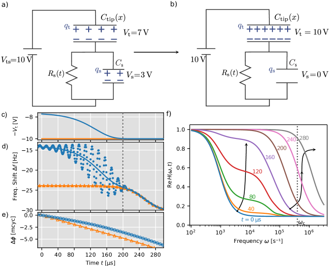
Figure S1: Frequency shift and time-varying transfer function versus time for a representative pk-EFM experiment. (a) The model circuit used in this simulation. After the tip-sample voltage is applied, charge builds up on the tip and sample capacitors. (b) Eventually, the sample capacitor discharges and $V_{\mathrm{t}}=V_{\mathrm{ts}}$. The (c) negative zeroth order tip voltage $-V_{\mathrm{t}}$, (d) frequency shift, and (e) phase shift calculated using numerical simulations (points) and analytically using Eq. LABEL:eq:frequency_shift_time_varying (line). For (c)–(e), $V_{\mathrm{t}}(t_{0})=$7\text{\,}\mathrm{V}$$ (blue circles), $10\text{\,}\mathrm{V}$ (orange triangles). (f) The time-varying response function $H(\omega,t)$ shown at times $t=$ 0, 40, 80, …, $280\text{\,}\mathrm{\SIUnitSymbolMicro s}$. Constant experimental parameters: $R_{\mathrm{dark}}=$10\text{\,}\mathrm{T\SIUnitSymbolOhm}$$, $R_{\mathrm{light}}=$10\text{\,}\mathrm{M\SIUnitSymbolOhm}$$, $\tau_{\mathrm{L}}=$40\text{\,}\mathrm{\SIUnitSymbolMicro s}$$, $k_{\mathrm{c}}=$3.5\text{\,}\mathrm{N}\text{\,}{\mathrm{m}}^{-1}$$, $f_{\mathrm{c}}=$62\text{\,}\mathrm{kHz}$$, $Q=$26\,000$$, $C_{\mathrm{tip}}=$1\text{\times}{10}^{-4}\text{\,}\mathrm{pF}$$, $C_{\mathrm{tip}}^{\prime}=$-2.8\text{\times}{10}^{-5}\text{\,}\mathrm{pF}\text{\,}{\mathrm{\SIUnitSymbolMicro m}}^{-1}$$, $C_{\mathrm{s}}=$1\text{\times}{10}^{-5}\text{\,}\mathrm{pF}$$, $C_{\mathrm{tip}}^{\prime\prime}=$6.77\text{\times}{10}^{-5}\text{\,}\mathrm{pF}\text{\,}{\mathrm{\SIUnitSymbolMicro m}}^{-2}$$, $V_{\mathrm{ts}}=$10\text{\,}\mathrm{V}$$, $t_{0}=$-200\text{\,}\mathrm{\SIUnitSymbolMicro s}$$.

Simulations were performed for a wide variety of experimental parameters, designed to cover regimes where each factor ($V_{\mathrm{t}}$ and $\operatorname{Re}{H(\omega_{\mathrm{c}},t)}$) influences the frequency shift. For sample tr-EFM experiments, Figure S2 shows that Eq. LABEL:eq:frequency_shift_time_varying is a good approximation of the cantilever frequency shift.

To assess pk-EFM experiments, the measured and predicted phase shifts were compared for 1080 simulated experiments. Figure S3 shows that over a wide variety of sample and cantilever parameters, the predicted and measured phase shift in pk-EFM experiments agreed closely. The residuals $r=\Delta\phi_{\mathrm{simulated}}-\Delta\phi_{\mathrm{predicted}}$ had a mean and standard deviation of $0.027\text{\,}\mathrm{mcyc}$ and $0.049\text{\,}\mathrm{mcyc}$ respectively. The maximum residual was $0.20\text{\,}\mathrm{mcyc}$.

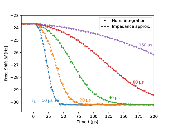
Figure S2: Frequency shift versus time for representative simulated EFM experiments. For different light-induced time constants $\tau_{\mathrm{L}}$ (Eq. S18), points show the frequency shift calculated from numerical integration of Eq. S20 and dashed lines show the results calculated using the approximation in Eq. LABEL:eq:frequency_shift_time_varying. For each trace, the following experimental parameters were held constant: $f_{\mathrm{c}}=$62.5\text{\,}\mathrm{kHz}$$, $k_{\mathrm{c}}=$3.5\text{\,}\mathrm{N}\text{\,}{\mathrm{m}}^{-1}$$, $Q=$26\,000$$, $A_{0}=$50\text{\,}\mathrm{nm}$$, $\phi_{0}=\pi$, $t_{0}=$-100\text{\,}\mathrm{\SIUnitSymbolMicro s}$$, $R_{\mathrm{dark}}=$100\text{\,}\mathrm{G\SIUnitSymbolOhm}$$, $R_{\mathrm{light}}=$10\text{\,}\mathrm{M\SIUnitSymbolOhm}$$, $C_{\mathrm{s}}=0$, $C_{\mathrm{tip}}=$1\text{\times}{10}^{-4}\text{\,}\mathrm{pF}$$, $C^{\prime\prime}_{q}=$52.1\text{\,}\mathrm{pF}\text{\,}{\mathrm{nm}}^{-2}$$, $\Delta C^{\prime\prime}=$15.7\text{\,}\mathrm{pF}\text{\,}{\mathrm{nm}}^{-2}$$, $V_{\mathrm{t}}(t_{0})=$10\text{\,}\mathrm{V}$$, $V_{\mathrm{ts}}=$10\text{\,}\mathrm{V}$$.

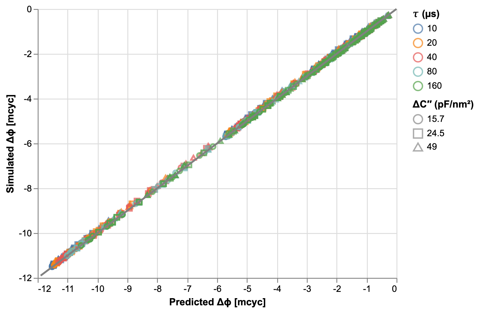
Figure S3: Simulated phase shift agrees closely with predicted phase shift in pk-EFM experiments. Experimental parameters: $R_{\mathrm{dark}}$ = $1\text{\times}{10}^{5}$, $1\text{\times}{10}^{7}$, $1\text{\times}{10}^{8}\text{\,}\mathrm{M\SIUnitSymbolOhm}$; $R_{\mathrm{light}}=$10\text{\,}\mathrm{M\SIUnitSymbolOhm}$$; $\tau_{\mathrm{L}}=$ 10, 20, 40, 80, $160\text{\,}\mathrm{\SIUnitSymbolMicro s}$; $V_{\mathrm{t}}(t_{0})=$ 7, $10\text{\,}\mathrm{V}$; $t_{\mathrm{p}}=$ 48, 96, 192, $384\text{\,}\mathrm{\SIUnitSymbolMicro s}$; $C_{\mathrm{s}}=$ $0.01$, $0.04$, $0.1\text{\,}\mathrm{fF}$; $C_{\mathrm{tip}}^{\prime}=$ $-28$, $-35$, $-49.5\text{\,}\mathrm{fF}\text{\,}{\mathrm{nm}}^{-1}$; $C_{\mathrm{tip}}=$ $0.1\text{\,}\mathrm{fF}$; $f_{\mathrm{c}}=$62.5\text{\,}\mathrm{kHz}$$; $k_{\mathrm{c}}=$3.5\text{\,}\mathrm{N}\text{\,}{\mathrm{m}}^{-1}$$; $Q=$26\,000$$, $A_{0}=$50\text{\,}\mathrm{nm}$$; $A_{0}=$50\text{\,}\mathrm{nm}$$; $t_{0}=$-200\text{\,}\mathrm{\SIUnitSymbolMicro s}$$; $\phi_{0}=0$.

S3A Numerical simulations

The numerical simulations used to generate Figs. S2– S3 were performed in Python. The code for these simulations is publicly available Dwyer et al. (2020). The coupled first-order ordinary differential equations that described the cantilever dynamics are

$$\dot{x} =v$$ (S20a)

$$\dot{v} =-\omega_{\mathrm{c}}^{2}x-\frac{\omega_{\mathrm{c}}}{Q}v+\frac{C_{\mathrm{tip}}^{\prime}(x)}{2mC_{\mathrm{tip}}(x)^{2}}q_{\mathrm{t}}^{2}$$ (S20b)

$$\dot{q}_{R} =-\frac{1}{R_{\mathrm{s}}(t)(C_{\mathrm{tip}}(x)+C_{\mathrm{s}})}q_{R}+\frac{C_{\mathrm{tip}}(x)}{R_{\mathrm{s}}(t)(C_{\mathrm{tip}}(x)+C_{\mathrm{s}})}V_{\mathrm{ts}}(t).$$ (S20c)

where $v$ is the cantilever velocity. For convenient comparison to the model developed above, the zeroth order charge was also computed using

$$\dot{q}_{R}^{(0)}=-\frac{1}{R_{\mathrm{s}}(t)(C+C_{\mathrm{s}})}q_{R}^{(0)}+\frac{C}{R_{\mathrm{s}}(t)(C+C_{\mathrm{s}})}V_{\mathrm{ts}}(t),$$ (S21)

where $C=C_{\mathrm{tip}}(0)$. The tip capacitance and its derivatives were given by $C_{\mathrm{tip}}(x)=C+C^{\prime}x+C^{\prime\prime}x^{2}/2$. In Eq. S20b, the tip charge $q_{\mathrm{t}}$ was calculated using Eq. S15. The numerical integration was performed in Python using Scipy’s odeint function, storing the state vector $\bm{y}=(x\,\,\,v\,\,\,q_{R}\,\,\,q_{R}^{(0)})^{T}$ every $1\text{\,}\mathrm{\SIUnitSymbolMicro s}$.

The initial state vector for the cantilever was

$$\bm{y}_{0}=\begin{pmatrix}x\\ v\\ q_{R}\\ q_{R}^{(0)}\end{pmatrix}=\begin{pmatrix}A_{0}\cos(\omega_{\mathrm{c}}t_{0}+\phi_{0})\\ A_{0}\omega_{\mathrm{c}}\sin(\omega_{\mathrm{c}}t_{0}+\phi_{0})\\ \beta\,CV\\ \beta\,CV\end{pmatrix},$$

where $A_{0}$ is the cantilever’s initial amplitude, $\phi_{0}$ is the cantilever’s initial phase, $t_{0}=$-100\text{\,}\mathrm{\SIUnitSymbolMicro s}$$ is the initial time the numerical integration was started, $\beta$ is the initial fraction of the tip sample voltage that drops across the tip capacitor, and the applied tip-sample voltage $V=$10\text{\,}\mathrm{V}$$ (Eq. S19).

The output of the numerical integration was used to determine the cantilever’s amplitude, phase, and frequency. The cantilever amplitude $A=\lvert z\rvert$ and phase $\phi=\arg{z}$ were calculated using the complex number

$$z=(x-x_{\mathrm{eq}})-jv/\omega_{\mathrm{c}}.$$ (S22)

where $x_{\mathrm{eq}}=C_{\mathrm{tip}}^{\prime}V_{\mathrm{ts}}^{2}/(2k_{\mathrm{c}})$. The amplitude and phase data were filtered by averaging over a single cantilever period (16 data points). The frequency shift was calculated by numerically differentiating the filtered phase shift (using second order central differences via numpy’s gradient function).

To compare the impedance theory approximation to the numerical integration, the zeroth order tip voltage $V_{\mathrm{t}}$ and the time-varying frequency response $H(\omega,t)$ must be known. The zeroth order tip voltage was calculated using Eq. S16 with $q_{R}=q_{R}^{(0)}$. To approximate $H(\omega,t)$, the double integral of Eq. LABEL:eq:time-varying-response was broken into pieces depending on the value of $t$ and $\omega_{\mathrm{fast}}(t)$. When $\omega_{\mathrm{fast}}\ll\omega_{\mathrm{c}}$, the necessary integral is oscillatory and decays slowly which makes converging a numerical approximation difficult. In this case, the integrand was sampled at points equally spaced through the cantilever cycle ($160$ points per cycle) and Simpson’s rule was used to compute the value of the integral.

S4 Scanning probe microscopy

The scanning probe microscopy set up used to perform different measurements here has been described in our previous reports Dwyer et al. (2017). Cantilever motion was detected using a fiber interferometer operating at $1490\text{\,}\mathrm{nm}$ (Corning SMF-28 fiber). The laser diode’s (QPhotonics laser diode QFLD1490-1490-5S) dc current was set using a precision current source (ILX Lightwave LDX-3620), and the current was modulated at radio frequencies using the input on the laser diode mount (ILX Lightwave LDM 4984, temperature-controlled with ILX Lightwave LDT-5910B). The interferometer light was detected with a 200-kHz bandwidth photodetector (New Focus model 2011, built-in high-pass filter set to $200\text{\,}\mathrm{kHz}$) and digitized at $1\text{\,}\mathrm{MHz}$ (National Instruments, PCI-6259). The cantilever was driven using a commercial PLL cantilever controller (RHK Technology, PLLPro2 Universal AFM controller) with PLL feedback loop integral gain $I$ $=$ $2.5\text{\,}\mathrm{Hz}$, proportional gain $P$ $=$ $-5\text{\,}\mathrm{\SIUnitSymbolDegree}\text{\,}\mathrm{Hz}$. The sample was illuminated from above with a fiber-coupled $405\text{\,}\mathrm{nm}$ laser (Thorlabs model LP405-SF10, held at $25\text{\,}\mathrm{\SIUnitSymbolCelsius}$ with a Thorlabs model TED200C temperature controller). The laser current was controlled using the external modulation input of the laser’s current controller (Thorlabs model LDC202, $200\text{\,}\mathrm{kHz}$ bandwidth). The light was coupled to the sample through a multimode, $50\text{\,}\mathrm{\SIUnitSymbolMicro m}$ diameter core, $0.22$ NA optical fiber (Thorlabs model FG050LGA). The intensity at sample surface was calculated based on an estimated spot size of $\approx$ $0.26\text{\,}{\mathrm{mm}}^{2}$

Implementation of broad band local dielectric spectroscopy has been described previously in Refs. 6 and 7. The procedure is reproduced below for reference. For amplitude modulation BLDS (Fig. LABEL:fig:frequency-BLDSb), we applied a time-dependent voltage to the cantilever tip :

$$V_{\mathrm{m}}(t)=V_{\mathrm{pp}}\left(\frac{1}{2}+\frac{1}{2}\cos(2\pi f_{\mathrm{am}}t)\right)\>\cos(2\pi f_{\mathrm{m}}t).$$ (S23)

In the experiments reported in the manuscript, $f_{\mathrm{m}}=$200\text{\,}\mathrm{Hz}$$ to $1.5\text{\,}\mathrm{MHz}$, $f_{\mathrm{am}}=$45\text{\,}\mathrm{Hz}$$, and the amplitude was set to $V_{\mathrm{pp}}=$6\text{\,}\mathrm{V}$$. The time-dependent voltage in Equation S23 was generated using a digital signal generator (Keysight 33600). The cantilever frequency shift was measured in real time using a phase-locked loop (PLL; RHK Technology, model PLLPro2 Universal AFM controller), the output of which was fed into a lock-in amplifier (LIA; Stanford Research Systems, model $830$). The LIA time constant and filter bandwidth were $300\text{\,}\mathrm{ms}$ and $$6\text{\,}\mathrm{dB}$/\mathrm{oct}$, respectively. At each stepped value of $f_{\mathrm{m}}$, a wait time of $1500\text{\,}\mathrm{ms}$ was employed, after which frequency-shift data were recorded for an integer number of frequency cycles corresponding to $\approx$2\text{\,}\sec$$ of data acquisition at each $f_{\mathrm{m}}$. The measurable $\Delta f_{\mathrm{BLDS}}$ primarily probes the response at $\omega_{\mathrm{m}}$ (Eq. S24).

$$\Delta f_{\mathrm{BLDS}}(\omega_{\mathrm{m}})=-\frac{f_{\mathrm{c}}V_{\mathrm{m}}^{2}}{16k}\Big{[}C^{\prime\prime}_{q}+\Delta C^{\prime\prime}\operatorname{Re}\Big{(}\hat{H}(\omega_{\mathrm{m}}+\omega_{\mathrm{c}})\\ +\hat{H}(\omega_{\mathrm{m}}-\omega_{\mathrm{c}})\big{)}\Big{]}\lvert\hat{H}(\omega_{\mathrm{m}})\rvert^{2}$$ (S24)

$\Delta f_{\mathrm{BLDS}}$ is related to the plotted voltage-normalized frequency shift $\alpha$ by Eq. S25.

$$\alpha=\frac{\Delta f_{\mathrm{BLDS}}(\omega_{\mathrm{m}})}{V_{\mathrm{m}}^{2}}.$$ (S25)

The $\Delta f_{\mathrm{BLDS}}$ frequency-shift signal was obtained from the LIA outputs as follows. From the (real) in-phase and out-of-phase voltage signals $V_{X}$ and $V_{Y}$, respectively, a single (complex signal) in hertz was calculated using the formula

$$Z_{\mathrm{Hz}}=\left(V_{x}+j\,V_{y}\right)\frac{S}{10}\times\sqrt{2}\times 20\,\frac{\text{Hz}}{\text{V}}$$ (S26)

From $Z_{\mathrm{Hz}}$ we calculate $\alpha$

$$\alpha=\frac{4\lvert Z_{\mathrm{Hz}}\rvert}{V_{\mathrm{pp}}^{2}}=\frac{8\sqrt{2}\,S\sqrt{V_{x}^{2}+V_{y}^{2}}}{V_{\mathrm{pp}}^{2}}.$$ (S27)

In frequency shift BLDS (Fig. LABEL:fig:frequency-BLDSa) described in Ref. 7, the applied waveform is not amplitude modulated at $45\text{\,}\mathrm{Hz}$ and instead an equal period ON/OFF amplitude-modulating is applied. The resultant frequency shift is calculated by software demodulation of the cantilever response by subtracting the average frequency shift during the ON period from the OFF period.

S4A tr-EFM and pk-EFM

Implementation and data work up details for tr-EFM and pk-EFM have been extensively described in Ref. 5 and Ref. 8 and is reproduced briefly below for reference. A commercial pulse and delay generator (Berkeley Nucleonics, BNC565) was used to generate tip voltage and light modulation pulses, as well as to turn off the cantilever drive voltage. The PLLPro2 generated the cantilever drive voltage and also output a $1\text{\,}\mathrm{V}$, phase-shifted sine wave copy of the cantilever oscillation, generated by an internal lock-in amplifier coupled to the phase-locked loop. A home built gated cantilever clock circuit converted this $1\text{\,}\mathrm{V}$ phase-shifted sine wave to a square wave, which was used as a clock for timing tip voltage and light pulses. A $5\text{\,}\mathrm{V}$ digital signal output by the National Instruments PCI-6259 gates the clock, controlling the start of the experiment. The BNC565 was used to trigger all signals relative to the cantilever clock. Cantilever drive was switched off ($2\text{\,}\mathrm{ms}10\text{\,}\mathrm{ms}$) before the start of light pulse. The raw cantilever oscillation data (digitized at 1 MHz) was saved along with counter timings (PCI-6259, 80-MHz counter) indicating the precise starting time of the light pulse (synchronized to the cantilever oscillation), allowing the start of the light pulse to be determined to within $12.5\text{\,}\mathrm{ns}$. Along with each pk-EFM phase shift data point, a control data point, identical except without turning on the light, was collected.

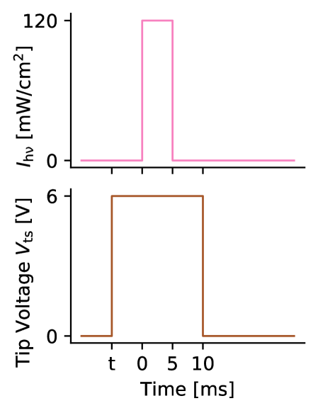
Figure S4: Timing diagram for voltage and light pulse used in Fig. LABEL:fig:trEFM-tp-time experiments. Bias time in dark $t$ is varied from $-2\text{\,}\mathrm{ms}$ to $-1000\text{\,}\mathrm{ms}$.

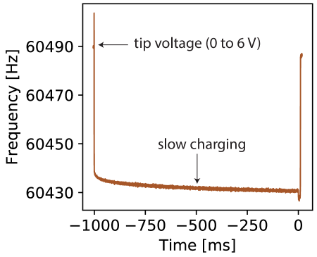
Figure S5: tr-EFM frequency shift for $t_{\mathrm{p}}$ $=$ $1\text{\,}\mathrm{s}$ shown in Fig. LABEL:fig:trEFM-tp-time. Additional frequency shift due to slow charging is apparent in the measured frequency shift after the tip voltage $V_{\mathrm{ts}}$ is changed to $6\text{\,}\mathrm{V}$ even after several hundred millisecond wait.

Figure S6: Dielectric response at $\omega_{\mathrm{m}}$ $=$ $1257\text{\,}{\mathrm{s}}^{-1}$ for a period of illumination at two different light intensities. Dielectric response measured by $\alpha$ increases and decreases within the time resolution of the measurement ($\approx$ $1\text{\,}\mathrm{s}$). Light was turned at time $t$ $=$ $20\text{\,}\mathrm{s}$ and turned off at time $t$ $=$ $52\text{\,}\mathrm{s}$. Experimental parameters: $V_{\mathrm{ts}}=$6\text{\,}\mathrm{V}$$, $h=$200\text{\,}\mathrm{nm}$$.

Figure S7: Surface potential measured through frequency voltage parabolas at selected light intensities.

Figure S8: Absorbance spectra of BA2PbI4.

Figure S9: AFM topography image of the perovskite film.

Figure S10: XRD spectra of the perovskite film.

References

• Giessibl (1997) F. J. Giessibl, Phys. Rev. B 56, 16010 (1997), [url].
• Dwyer et al. (2019) R. P. Dwyer, L. E. Harrell, and J. A. Marohn, Phys. Rev. Applied 11, 064020 (2019), [url].
• Kailath (1980) T. Kailath, Linear Systems (Prentice-Hall, Inc., Englewood Cliffs, N.J, 1980), 1st ed.
• Shmaliy (2007) Y. Shmaliy, Continuous-Time Systems (SPRINGER NATURE, 2007).
• Dwyer et al. (2017) R. P. Dwyer, S. R. Nathan, and J. A. Marohn, Sci. Adv. 3, e1602951 (2017), [url].
• Tirmzi et al. (2017) A. M. Tirmzi, R. P. Dwyer, T. Hanrath, and J. A. Marohn, ACS Energy Lett. 2, 488 (2017), [url].
• Tirmzi et al. (2019) A. M. Tirmzi, J. A. Christians, R. P. Dwyer, D. T. Moore, and J. A. Marohn, J. Phys. Chem. C 123, 3402 (2019), [url].
• Dwyer (2017) R. P. Dwyer, Ph.D. thesis, Cornell University, Ithaca, New York (2017).
• Dwyer et al. (2020) R. P. Dwyer, A. M. Tirmzi, and J. A. Marohn, Numerical simulations and theory for “Light-dependent Impedance Spectra and Transient Photoconductivity in a Ruddlesden–Popper 2D Lead-halide Perovskite Revealed by Electrical Scanned probe Microscopy and Accompanying Theory”, Available from https://github.com/ryanpdwyer/light-dependent-impedance-spectra (2020), [url].