Attack-Resilient State Estimation with Intermittent Data Authentication

Abstract

Network-based attacks on control systems may alter sensor data delivered to the controller, effectively causing degradation in control performance. As a result, having access to accurate state estimates, even in the presence of attacks on sensor measurements, is of critical importance. In this paper, we analyze performance of resilient state estimators (RSEs) when any subset of sensors may be compromised by a stealthy attacker. Specifically, we consider systems with the well-known $l_{0}$-based RSE and two commonly used sound intrusion detectors (IDs). For linear time-invariant plants with bounded noise, we define the notion of perfect attackability (PA) when attacks may result in unbounded estimation errors while remaining undetected by the employed ID (i.e., stealthy). We derive necessary and sufficient PA conditions, showing that a system can be perfectly attackable even if the plant is stable. While PA can be prevented with the use the standard cryptographic mechanisms (e.g., message authentication) that ensure data integrity under network-based attacks, their continuous use imposes significant communication and computational overhead. Consequently, we also study the impact that even intermittent use of data authentication has on RSE performance guarantees in the presence of stealthy attacks. We show that if messages from some of the sensors are even intermittently authenticated, stealthy attacks could not result in unbounded state estimation errors.

,

1 Introduction

The challenge of securing control systems has recently attracted significant attention due to high profile attacks, such as the attack on Ukrainian power grid [25] and the StuxNet attack [8]. In such incidents, the attacker can affect a physical plant by altering actuation commands or sensory measurements, or affecting execution of the controller. One approach to address this problem has been to exploit a dynamical model of the plant for attack detection and attack-resilient control (e.g., [12, 24, 19, 1, 18, 14, 15, 23, 6]).

For instance, consider the problem of attack-resilient control when measurements from a subset of the plant sensors may be compromised. One line of work employs a widely used (non-resilient) Kalman filter, with a standard residual-based probabilistic detector (e.g., $\mathcal{X}^{2}$ detector) triggering alarm in the presence of attack [24, 7, 3]. These Kalman filter-based controllers of linear time-invariant (LTI) plants may be vulnerable to stealthy (i.e., undetected) attacks resulting in unbounded state-estimation errors; thus, such systems are referred to as perfectly attackable (PA) [24, 7, 3]. Specifically, for LTI systems with Gaussian noise and Kalman filter-based controllers, the notion of perfect attackability (PA) is introduced in [24]. In particular, [24], and [3] for larger classes of intrusion detectors (IDs), show that the system is PA if and only if the plant is unstable and the set of compromised sensors satisfies that no unstable eigenvector lie in the kernel of their observation matrix.

Resilient (i.e., secure) state estimation is another approach to achieve attack-resilient control; here, the objective is to estimate the system state when a subset of the sensors is corrupted [1, 16]. This allows for the use of standard feedback controllers to provide strong control guarantees in the presence of attacks. A common approach is to use a batch-processing resilient state estimator (RSE) to estimate the system state and attack vectors (e.g., [1, 15, 14, 18]). For LTI systems without noise, the state and attack vectors can be obtained by solving an $l_{0}$, or under more restrictive condition $l_{1}$, optimization problem [1]. These results are extended to systems with bounded noise [14], showing that the worst case state estimation error is a linear with the noise size; thus, the attacker cannot exploit the noise to introduce unbounded state-estimation errors, unless a sufficiently large number of sensors is corrupted. SMT- and graph-based estimators from [18] and [11] improve computational efficiency of the estimators. However, all these methods employ a common restrictive assumption that the maximal number of corrupted sensors is bounded; at best, less than half of sensors can be compromised. Moreover, to the best of our knowledge, the impact of stealthy attacks on the RSEs has not been considered, either in the general case or under such restrictive assumptions.

However, the assumption that measurements from only a subset of sensors are compromised cannot be justified in the common scenarios where the attacker has access to the network used to transmit data from sensors to the controller. Thus, it is important to analyze impact of such Man-in-the-Middle attacks on performance of the RSEs. A common defense against network-based attacks is the use of cryptographic tools, such as adding Message Authentication Codes (MACs) to measurement messages to guarantee their integrity. Yet, continuous use of security primitives such as MACs, can cause computation and communication overhead, which limits its applicability in resource-constrained control systems [9, 10]. To overcome this, intermittent data authentication can be used for control systems [3]; specifically, LTI systems with Gaussian noise and a Kalman filter-based controller, cannot be PA if message authentication is at least intermittently employed. On the other hand, no such guarantees have been shown in systems with bounded-size noise and RSE-based controllers.

Consequently, in this work, we focus on performance of LTI systems with bounded-size noise, employing an RSE-based controller, under stealthy attacks on an arbitrary number of sensors. Specifically, we consider a system with an $l_{0}$-based RSE, due to the strongest resiliency guarantees, and one of two previously reported intrusion detectors (IDs) for systems with set-based noise. Due to the batch-processing nature of RSEs, we introduce two notions of PA for such systems – at a single time point and over time, where a stealthy attacker may introduce arbitrarily large estimation errors. Then, we provide necessary and sufficient conditions for both notions of PA. We show that unlike PA in the Kalman filter-based estimators, a system may be PA over time even if the physical plant is not unstable. Furthermore, we show that even intermittent data authentication guarantee can help against such perfect attacks for some types of IDs. Unlike [3], we show that using authentication only once in every bounded time interval ensures bounded estimation errors under any stealthy attack.

This paper is organized as follows. Section 2 formalizes the problem including the system and attack models. In Section 3, we define the concept of perfectly attackable systems and find the necessary and sufficient conditions for PA. In Section 4, we study effects of intermittent message authentication on performance guarantees under attack. Finally, our results are illustrated in case studies in Section 5, before concluding remarks in Section 6.

Notation. $\mathbb{B}$ and $\mathbb{R}$ denote the set of Boolean and real numbers, respectively, and $\mathbb{I}(.)$ is the indicator function. For a matrix $A$, $\mathcal{N}(A)$ denotes its null space, $A^{T}$ its transpose, $A^{\dagger}$ its Moore-Penrose pseudoinverse, and $||A||$ the $l_{2}$ norm of the matrix. For a vector $x\in{\mathbb{R}^{n}}$, we denote by $||x||_{p}$ the $p$-norm of $x$; when $p$ is not specified, the 2-norm is implied. In addition, we use $x_{i}$ to denote the $i^{\text{th}}$ element of $x$, while $\text{supp}(x)$ denotes the indices of nonzero elements of $x$ – i.e., $\text{supp}(x)=\{i~{}|~{}i\in\{1,...,n\},x_{i}\neq 0\}$.

Projection vector $e_{i}$ is the unit vector where a 1 in its $i^{th}$ position is the only nonzero element of the vector. For set $\mathcal{S}$, $|\mathcal{S}|$ denotes the cardinality of the set and $\mathcal{S}^{\complement}$ its complement. $\mathcal{P}_{\mathcal{K}}x$ is the projection from the set $\mathcal{S}$ to set $\mathcal{K}$ ($\mathcal{K}\subseteq\mathcal{S}$) by keeping only elements of $x$ with indices from $\mathcal{K}$; formally, $\mathcal{P}_{\mathcal{K}}=\left[\begin{smallmatrix}e_{j_{1}}|\ldots|e_{j_{|\mathcal{K}|}}\end{smallmatrix}\right]^{T}$, where $\mathcal{K}=\{s_{j_{1}},...,s_{j_{|\mathcal{K}|}}\}\subseteq{S}$ and $j_{1}<j_{2}<...<j_{|\mathcal{K}|}$. If e.g., $\mathcal{S}=\{1,2,3,4\}$ and $\mathcal{K}=\{2,4\}$, then $\mathcal{P}_{\mathcal{K}}x=\left[\begin{smallmatrix}x_{2}&x_{4}\end{smallmatrix}\right]^{T}$.

2 Problem Description

We start by introducing the system (Fig. 1) and attack model, before formalizing the considered problem.

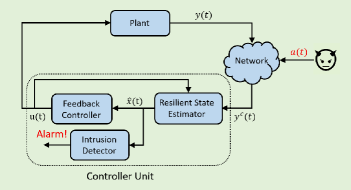
Figure 1: Control architecture under network-based attacks.

2.1 System and Attack Model

We now describe each system component from Fig. 1.

Plant Model. We assume that the plant is an observable linear time-invariant (LTI) dynamical system that can be modeled in the standard state-space form as

$$\begin{split}x(t+1)&=Ax(t)+Bu(t)+v_{P}(t),\\ y(t)&=Cx(t)+v_{M}(t).\end{split}$$ (1)

Here, $x\in{\mathbb{R}^{n}}$, $u\in{\mathbb{R}^{m}}$, $y\in{\mathbb{R}^{p}}$ denote the state, input and output vectors, respectively. The plant output vector captures measurements from the set of plant sensors $\mathcal{S}=\{s_{1},s_{2},...,s_{p}\}$. In addition, $v_{P}\in{\mathbb{R}^{n}}$ and $v_{M}\in{\mathbb{R}^{p}}$ are bounded process and measurement noise vectors – i.e., there exist $\delta_{v_{P}},\delta_{v_{M}}\in\mathbb{R}$ such that for all $t\geq{0}$,

$$\left\lVert v_{P}(t)\right\rVert_{2}\leq{\delta_{v_{P}}},\quad\left\lVert v_{M}(t)\right\rVert_{2}\leq{\delta_{v_{M}}}.$$ (2)

Note that we make no assumptions about the distributions of the sensor and measurement noise models.

Attack Model. We assume that the attacker was able to compromise information flow from a subset of sensors $\mathcal{K}\subseteq{\mathcal{S}}$; however, we make no assumption about the set $\mathcal{K}$ (e.g., its size or elements). Hence, the sensor measurements delivered to the controller can be modeled as

$$y^{c}(t)=y(t)+a(t).$$ (3)

Here, $a(t)\in{\mathbb{R}^{p}}$ denotes the sparse attack signal injected by the attacker at time $t$ via the compromised information flows (i.e., sensors) from $\mathcal{K}$; hence, $\mathcal{K}=\text{supp}(a(t))$.

We use a commonly adopted threat model (e.g., [3]) where:

1. the attacker has the full knowledge of the system, its dynamics and design (e.g., controller and ID), as well as the employed security mechanisms – e.g., the times when authentication is used,

2. the attacker has the required computation power to calculate suitable attack signals to inject via the set $\mathcal{K}$, while planning ahead as needed,

3. the attacker’s goal is to design attack signal $a(t)$ such that it always remain stealthy (i.e., undetected by the ID), while maximizing control degradation.

The notions of stealthiness and control performance degradation depend on the controller, and thus will be formally defined after the controller design is introduced.

Controller Design. The controller employs an RSE whose output is used for standard feedback control, and an ID (Fig. 1). To simplify our notation while describing the RSE, the model (1) can be considered in the form

$$\begin{split}x(t+1)&=Ax(t),\\ y(t)=y^{c}(t)&=Cx(t)+w(t)+a(t);\end{split}$$ (4)

specifically, we can ignore the contribution of $u(t)$ as it is a known signal (no attacks on actuator are considered in this work) and thus has no effect on resilient state estimation. As shown in [13, 14], the bounds on the size of measurement noise $w$ in (4) can be related to the bounds on the size of process and measurement noise vectors $v_{P}$ and $v_{M}$; i.e., there exists $\delta_{w}>0$ such that

$$||w(t)||\leq\delta_{w},\qquad\text{for all }~{}t\geq 0.$$ (5)

Resilient State Estimator. The goal of an RSE is to reconstruct the system state $x(t)$ from $N$ sensor measurements $\{y(t),...,y(t+N-1)\}$. We assume that $N=n$; however, the results can be extended to the case $N<n$, or $N>n$. To formally capture RSE requirements, we rewrite the system model from (4) as

$${\mathbf{y}}(t)=\mathbf{O}x(t)+\mathbf{a}(t)+{\mathbf{w}}(t),$$ (6)

where $\mathbf{O}=[\mathbf{O}_{1}^{T}~{}|~{}...~{}|~{}\mathbf{O}_{p}^{T}]^{T}$. For each sensor $i$ and a subset of sensors $\mathcal{K}$, we define the matrices $\mathbf{O}_{i}$ and $\mathbf{O}_{\mathcal{K}}$ as

$$\mathbf{O}_{\mathcal{K}}=\begin{bmatrix}(\mathcal{P}_{\mathcal{K}}C)^{T}&(\mathcal{P}_{\mathcal{K}}CA)^{T}&\dots&(\mathcal{P}_{\mathcal{K}}CA^{N-1})^{T}\end{bmatrix}^{T},$$ (7)

with $\mathbf{O}_{i}=\mathbf{O}_{\{s_{i}\}}$. Also, each of the block vectors $\mathbf{a}$, ${\mathbf{y}}$, ${\mathbf{w}}\in{\mathbb{R}^{pN}}$, satisfies $\mathbf{a}(t)=[\mathbf{a}_{1}^{T}(t)~{}|~{}...~{}|~{}\mathbf{a}_{p}^{T}(t)]^{T}$, ${\mathbf{y}}(t)=[{\mathbf{y}}_{1}^{T}(t)~{}|~{}...~{}|~{}{\mathbf{y}}_{p}^{T}(t)]^{T}$ and ${\mathbf{w}}(t)=[{\mathbf{w}}_{1}^{T}(t)~{}|~{}...~{}|~{}{\mathbf{w}}_{p}^{T}(t)]^{T}$. Now, for each sensor $i\in{\mathcal{S}}$, it holds that

$${\mathbf{y}}_{i}(t)=\mathbf{O}_{i}x(t)+\mathbf{a}_{i}(t)+{\mathbf{w}_{i}}(t)$$ (8)

with ${\mathbf{a}}_{i}(t)=[a_{i}(t)~{}|~{}a_{i}(t+1)~{}|...|~{}a_{i}(t+N-1)]^{T}\in{\mathbb{R}^{N}}$ denoting the values injected via $i^{\text{th}}$ sensor at time steps $t,...,t+N-1$, with ${\mathbf{a}}_{i}(t)=0$ if $i\notin{\mathcal{K}}$. Finally, ${{\mathbf{y}}}_{i}(t)=[y_{i}(t)~{}|~{}y_{i}(t+1)~{}|...|~{}y_{i}(t+N-1)]^{T}\in{\mathbb{R}^{N}}$ and ${{\mathbf{w}}}_{i}(t)=[w_{i}(t)~{}|~{}w_{i}(t+1)~{}|...|~{}w_{i}(t+N-1)]^{T}\in{\mathbb{R}^{N}}$ are the values of sensor $i$ measurements and its noise.

In general, the RSE functionality can be captured as [1]

$$\mathcal{E}:\mathbb{R}^{Np}\mapsto\mathbb{R}^{n}\times\mathbb{R}^{Np}~{}~{}s.t.\quad\mathcal{E}({\mathbf{y}}(t))=\big{(}\hat{x}(t),{\hat{\mathbf{a}}}(t)\big{)}.$$ (9)

Here, $\hat{x}(t)$ and ${\hat{\mathbf{a}}}(t)$ are the state and attack vectors estimated from the delivered sensor measurements. The estimation error of an RSE is defined as

$$\Delta x(t)=\hat{x}(t)-x(t).$$ (10)

A conventional RSE is the $l_{0}$-based decoder [14], or its equivalent forms (e.g., [1, 18]), defined as optimization

$$\begin{split}&\min\limits_{\hat{x}(t),{\hat{\mathbf{a}}}(t)}\sum\nolimits_{i=1}^{p}\mathbb{I}\big{(}\left\lVert{\hat{\mathbf{a}}}_{i}(t)\right\rVert>0\big{)}\\ &s.\,\,t.\,\,\,\,\,{\mathbf{y}}(t)=\mathbf{O}\hat{x}(t)+\hat{{\mathbf{w}}}(t)+\hat{\mathbf{a}}(t)\\ &\,\,\,\,\,\,\,\,\,\,\,\,\,\,\,{\hat{{\mathbf{w}}}(t)}\in{\Omega}.\end{split}$$ (11)

Here, $\Omega$ denotes the feasible set of noise vectors, determined by the noise bounds from (5). The vectors ${\hat{{\mathbf{w}}}(t)}$ and ${\hat{{\mathbf{a}}}(t)}$ are estimated at time $t$ independently from the estimated vectors at time step $t-1$. Hence, we denote ${\hat{{\mathbf{w}}}(t)}=[{\hat{\mathbf{w}}}_{1}^{T}(t)~{}|~{}...~{}|~{}\hat{{\mathbf{w}}}_{p}^{T}(t)]^{T}$, ${\hat{{\mathbf{a}}}(t)}=[{\hat{\mathbf{a}}}_{1}^{T}(t)~{}|~{}...~{}|~{}{\hat{\mathbf{a}}}_{p}^{T}(t)]^{T}$, with ${\hat{\mathbf{w}}}_{i}(t)=[\hat{w}^{(t)}_{i}(t)|...|\hat{w}^{(t)}_{i}(t+N-1)]^{T}$ and ${\hat{\mathbf{a}}}_{i}(t)=[\hat{a}^{(t)}_{i}(t)|...|\hat{a}^{(t)}_{i}(t+N-1)]^{T}$, in which $\hat{a}^{(t)}_{i}(k)$ and $\hat{w}^{(t)}_{i}(k)$ are the estimated noise and attack vectors at time $k$, as computed at time $t$, for $k=t,...,t+N-1$.

When not more than $s$ sensors are compromised in a $2s$-sparse observable system [17], the estimation error of the RSE (11) is bounded [14]; $2s$-sparse observable depends on the properties of the observability matrix of $(A,C)$.

Intrusion Detector. We consider two ID used to detect the presence of any system anomaly (including attacks):

1. ID${}_{\textit{\@slowromancap i@}}$: We capture the ID${}_{\@slowromancap}i@$ functionality in the general form as mapping $\mathcal{D}_{\textit{\@slowromancap i@}}:\mathbb{R}^{Np}\mapsto\mathbb{B}$ defined as

   $$\mathcal{D}_{\textit{\@slowromancap i@}}(\hat{\mathbf{a}}(t))=\mathbb{I}(\left\lVert\hat{\mathbf{a}}(t)\right\rVert>0);$$ (12)

   i.e., if the estimated attack vector is non-zero, ID${}_{\textit{\@slowromancap i@}}$ raises alarm. Note that our goal is not to identify the exact set of attacked sensors, which would result in a nonzero threshold in (12), as shown in [14].

2. ID${}_{\textit{\@slowromancap ii@}}$: We define the ID${}_{\textit{\@slowromancap ii@}}$ as $\mathcal{D}_{\textit{\@slowromancap ii@}}:\mathbb{R}^{Np+2n}\mapsto\mathbb{B}$ with

   $$\begin{split}&\mathcal{D}_{\textit{\@slowromancap ii@}}(\hat{\mathbf{a}}(t),\hat{x}(t),\hat{x}(t-1))=\\ &\mathbb{I}\big{(}\left\lVert\hat{\mathbf{a}}(t)\right\rVert>0\big{)}\lor\mathbb{I}\big{(}||\hat{x}(t)-A\hat{x}(t-1)||>{d}\big{)};\end{split}$$ (13)

   here, $\lor$ is Boolean OR and $d$ is defined by Prop. 1.

We use $\mathcal{D}_{\textit{\@slowromancap i@}}(\hat{\mathbf{a}})$ and $\mathcal{D}_{\textit{\@slowromancap ii@}}(\hat{\mathbf{a}},\hat{x})$ instead of $\mathcal{D}_{\textit{\@slowromancap i@}}(\hat{\mathbf{a}}(t))$ and $\mathcal{D}_{\textit{\@slowromancap ii@}}(\hat{\mathbf{a}}(t),\hat{x}(t),\hat{x}(t-1))$, respectively. We also denote the system (4) with ID${}_{\textit{{i}}}$ ($\textit{{i}}\in\{$ i@, ii@$\}$) as $\Sigma_{\textit{i}}(A,C,\delta_{w},\mathcal{K})$. Yet, if results hold for both IDs, we remove the subscript i.

Proposition 1.

For the system without attack, it holds that $||\hat{x}(t)-A\hat{x}(t-1)||\leq d=2\sqrt{N}\delta_{w}||\mathbf{O}^{\dagger}||_{2}(1+||A||_{2})$.

Constraints in (11) at time $t$ and $t-1$ imply

$$\begin{split}\mathbf{O}{x}(t)+{\mathbf{w}}(t)=&\mathbf{O}\hat{x}(t)+\hat{{\mathbf{w}}}(t)\\ \mathbf{O}{x}(t-1)+{\mathbf{w}}(t-1)=&\mathbf{O}\hat{x}(t-1)+\hat{{\mathbf{w}}}(t-1)\end{split}$$ (14)

For $\Delta{\mathbf{w}}(t)={\mathbf{w}}(t)-\hat{{\mathbf{w}}}(t)$, since $(A,C)$ is observable,

$$\begin{split}\hat{x}(t)=&x(t)-\mathbf{O}^{\dagger}\Delta{{\mathbf{w}}}(t)\\ \hat{x}(t-1)=&x(t-1)-\mathbf{O}^{\dagger}\Delta{{\mathbf{w}}}(t-1).\end{split}$$ (15)

Hence, from (4), $||\hat{x}(t)-A\hat{x}(t-1)||=||A\mathbf{O}^{\dagger}\Delta{{\mathbf{w}}}(t-1)-\mathbf{O}^{\dagger}\Delta{{\mathbf{w}}}(t)||\leq||\mathbf{O}^{\dagger}||_{2}||\Delta{{\mathbf{w}}}(t)||+||A||_{2}||\mathbf{O}^{\dagger}||_{2}||\Delta{{\mathbf{w}}}(t-1)||.$ On the other hand, $||\Delta{{\mathbf{w}}}(t)||_{2}\leq 2\sqrt{N}\delta_{w}$, which also holds for $\Delta{{\mathbf{w}}}(t-1)$, and thus concludes the proof.

2.2 Problem Formulation

In this work, we focus on the following two problems.

Problem 1: Under which conditions, a stealthy attacker could introduce arbitrarily large estimation errors (10)? From (12), (13), the stealthiness conditions for ID${}_{\textit{\@slowromancap i@}}$, ID${}_{\textit{\@slowromancap ii@}}$ are

$$\mathcal{D}_{\textit{\@slowromancap i@}}(\hat{\mathbf{a}})=0,\qquad\mathcal{D}_{\textit{\@slowromancap ii@}}(\hat{\mathbf{a}},\hat{x})=0.$$ (16)

Note that if an attack is stealthy from ID${}_{\textit{\@slowromancap ii@}}$ it cannot be detected by ID${}_{\textit{\@slowromancap i@}}$ either. Due to the batch-processing nature of the RSE and bounded-size noise, the approach and conditions from [24, 7] cannot be used. Hence, we introduce PA for LTI systems with bounded-size noise.

Problem 2: As we show in next section, for a large class of systems $\Sigma_{\textit{\@slowromancap i@}}(A,C,\delta_{w},\mathcal{K})$, an unbounded state estimation error can be inserted by compromising a subset of sensors. Although the use of ID${}_{\textit{\@slowromancap ii@}}$ (i.e., for systems $\Sigma_{\textit{\@slowromancap ii@}}(A,C,\delta_{w},\mathcal{K})$) restricts these conditions, unstable plants are vulnerable to perfect attacks (i.e., stealthy attacks that cause unbounded estimation errors). On the other hand, the use of security mechanisms, such as message authentication, could ensure integrity of the received sensor measurements. Thus, a stealthy attack vector has to satisfy $a_{i}(t)=0$ when the measurement of sensor $s_{i}$ is authenticated at time $t$, and ${a}(t)=0$ if integrity of all sensors is enforced at time $t$. Since authentication comes with additional computational and communication cost, we study the effects of intermittent data authentication on attack impact. Our goal is to find conditions that the authentication policy (i.e., times when authentication is used) should satisfy so that the systems $\Sigma_{\textit{\@slowromancap i@}}(A,C,\delta_{w},\mathcal{K})$, $\Sigma_{\textit{\@slowromancap ii@}}(A,C,\delta_{w},\mathcal{K})$ are not PA.

3 PA of LTI Systems with Bounded-Noise

The notion of PA is introduced in [24, 7] for systems with a statistical ($\chi^{2}$) ID and a Kalman-filter implementing continuous (i.e., streamed) processing of sensor measurements. On the other hand, most existing RSEs for systems with bounded noise (e.g., [14, 18, 21, 20]) are based on batch-processing of sensor data – i.e., processing a window of sensor measurements at each time step (mostly even without taking previous computations into account). Thus, the notion of PA needs to differentiate between PA at a single time point vs. PA over a time interval. In this section, we first define these two notions of PA for systems with one of the two IDs, before providing the necessary and sufficient conditions individually.

Definition 1.

System $\Sigma_{\textit{\@slowromancap i@}}(A,C,\delta_{w},\mathcal{K})$ is perfectly attackable at a single time step if for any $M>0$, there exists a stealthy sequence of attack signals $\mathbf{a}(t)$ over $N$ time steps (i.e., satisfying (16)), for which the RSE estimation error satisfies $||\Delta{x}(t)||>M$. Such attack vector $\mathbf{a}(t)$ is called a perfect attack for the system $\Sigma_{\textit{\@slowromancap i@}}(A,C,\delta_{w},\mathcal{K})$.

Definition 1 does not require that the attack is stealthy before or remains stealthy at time steps after $t$. Such notion of PA for the system $\Sigma_{\textit{\@slowromancap ii@}}(A,C,\delta_{w},\mathcal{K})$ is not relevant because the ID${}_{\textit{\@slowromancap ii@}}$, from (13), validates that the estimated states in every two consecutive steps do not violate plant dynamics. Thus, we characterize a more realistic requirements for stealthy attacks – PA over a time-interval.

Definition 2.

System $\Sigma(A,C,\delta_{w},\mathcal{K})$ is perfectly attackable over time if for all $M>0$ there exists a sequence of attack signals $\mathbf{a}(t),\mathbf{a}(t+1),...$ and a time point $t^{\prime}\geq t$ such that for all $k$, where $k\geq t^{\prime}$, it holds that $||\Delta{x}(k)||>M$, and for all time steps, the estimated attack vectors $\hat{\mathbf{a}}$ satisfies the corresponding stealthiness requirements in (16).

To simplify our presentation, instead of formally stating that the estimation error may be arbitrarily large, we may say that the estimation error is unbounded.

Remark 1.

If the system $\Sigma_{\textit{\@slowromancap ii@}}(A,C,\delta_{w},\mathcal{K})$ is perfectly attackable over time, then the $\Sigma_{\textit{\@slowromancap i@}}(A,C,\delta_{w},\mathcal{K})$ is also perfectly attackable over time because the stealthiness condition in (16) for ID${}_{\textit{\@slowromancap ii@}}$ also includes the condition for ID${}_{\textit{\@slowromancap i@}}$.

Note that PA over time is a stronger notion than PA at a single time point because $\mathcal{D}_{\textit{\@slowromancap i@}}\big{(}\hat{\mathbf{a}}(t))\big{)}$ should be equal to zero for all time steps. Therefore, the following holds.

Proposition 2.

If the system $\Sigma_{\textit{\@slowromancap i@}}(A,C,\delta_{w},\mathcal{K})$ is PA over time, then it is also PA at a single time step.

3.1 PA of $\Sigma_{\textit{\@slowromancap i@}}(A,C,\delta_{w},\mathcal{K})$ System

We now capture conditions for PA at a single time.

Theorem 1.

System $\Sigma_{\textit{\@slowromancap i@}}(A,C,\delta_{w},\mathcal{K})$ is PA at a singletime step if and only if pair $(A,\mathcal{P}_{\mathcal{K}^{\complement}}C)$ is not observable.

($\Rightarrow$) Let us assume that the pair $(A,\mathcal{P}_{\mathcal{K}^{\complement}}C)$ is observable, while the system $\Sigma_{\textit{\@slowromancap i@}}(A,C,\delta_{w},\mathcal{K})$ is PA at a single time step, which we denote as $t$. Then, there exists a stealthy attack sequence ${\mathbf{a}}(t)$ for which the RSE estimated attack vector $\hat{\mathbf{a}}(t)=0$ and $\left\lVert\Delta{x}(t)\right\rVert$ is unbounded.

Consider data from noncompromised sensors in $\mathcal{K}^{\complement}$; i.e.,

$$\mathcal{P}_{\mathcal{K}^{\complement}}\mathbf{y}(t)\overset{\text{\small(i)}}{=}\mathbf{O}_{\mathcal{K}^{\complement}}x(t)+\mathcal{P}_{\mathcal{K}^{\complement}}{\mathbf{w}}(t)\overset{\text{\small(ii)}}{=}\mathbf{O}_{\mathcal{K}^{\complement}}\hat{x}(t)+\mathcal{P}_{\mathcal{K}^{\complement}}\hat{{\mathbf{w}}}(t),$$

where (i) holds from (6) as the sensors are noncompromised, whereas (ii) holds from (11) since the attack is stealthy (i.e., $\hat{\mathbf{a}}(t)=0$). Hence, it follows that $\mathbf{O}_{\mathcal{K}^{\complement}}\Delta{x}(t)=\mathcal{P}_{\mathcal{K}^{\complement}}\Delta{\mathbf{w}}(t),$ where $\Delta{\mathbf{w}}(t)={\mathbf{w}}(t)-\hat{{\mathbf{w}}}(t)$. Since the matrix $\mathbf{O}_{\mathcal{K}^{\complement}}$ is full rank, $\Delta{x}(t)=\big{(}\mathbf{O}_{\mathcal{K}^{\complement}}\big{)}^{\dagger}\Big{(}\mathcal{P}_{\mathcal{K}^{\complement}}\Delta{\mathbf{w}}(t)\Big{)},$ and thus

$$\begin{split}\left\lVert\Delta{x}(t)\right\rVert\leq&\left\lVert\big{(}\mathbf{O}_{\mathcal{K}^{\complement}}\big{)}^{\dagger}\right\rVert\Big{(}\left\lVert\mathcal{P}_{\mathcal{K}^{\complement}}\Delta{\mathbf{w}}(t)\right\rVert\Big{)}.\end{split}$$ (17)

The matrix $\big{(}\mathbf{O}_{\mathcal{K}^{\complement}}\big{)}^{\dagger}$ has a bounded norm, $\mathbf{w}(t)$ and $\hat{\mathbf{w}}(t)$ are also bounded. Thus, the right side of (17) is bounded, meaning that $\Delta x(t)$ is bounded, which is a contradiction.

($\Leftarrow$) Suppose that the pair $(A,\mathcal{P}_{\mathcal{K}^{\complement}}C)$ is not observable; thus, there exists a nonzero vector ${z}$ such that $\mathbf{O}_{\mathcal{K}^{\complement}}{z}=0$. Let us assume that the system is in state $x(t)$ when attack ${\mathbf{a}}(t)=\begin{bmatrix}(\mathcal{P}_{\mathcal{K}}{\mathbf{a}}(t))^{T}&(\mathcal{P}_{\mathcal{K}^{\complement}}{\mathbf{a}}(t))^{T}\end{bmatrix}^{T}=\mathbf{O}{z}=\begin{bmatrix}(\mathbf{O}_{\mathcal{K}}z)^{T}&0\end{bmatrix}^{T}$ is applied. Then, from (6) we have that

$${\mathbf{y}}(t)=\mathbf{O}{x}(t)+{{\mathbf{w}}}(t)+{\mathbf{a}}(t)=\mathbf{O}\hat{x}(t)+\hat{{\mathbf{w}}}(t)+\hat{\mathbf{a}}(t).$$ (18)

Consider $\hat{{\mathbf{w}}}^{\prime}(t)=\hat{{\mathbf{w}}}(t)$, $\hat{x}^{\prime}(t)=\hat{x}(t)+z$ and $\hat{\mathbf{a}}^{\prime}(t)=0$. Now, $\left(\hat{{{x}}}^{\prime}(t),\hat{{\mathbf{w}}}^{\prime}(t),\hat{{\mathbf{a}}}^{\prime}(t)\right)$ is a feasible point for the RSE optimization problem from (11) that also minimizes the objective to zero. Thus, the output of RSE $\left(\hat{x}(t),\hat{\mathbf{a}}(t)\right)$ also has to have the same value for the objective function – i.e., $\hat{\mathbf{a}}=\mathbf{0}$, and the attack will not be detected.

Since $(A,C)$ is observable, from (18) and (10), we have $\Delta x(t)=\mathbf{O}^{\dagger}\Delta{\mathbf{w}}(t)+\mathbf{O}^{\dagger}\mathbf{a}(t)=\mathbf{O}^{\dagger}\Delta{\mathbf{w}}(t)+z.$ As $\Delta{\mathbf{w}}(t)$ is bounded, and ${z}$ is any nonzero vector in the null-space of $\mathbf{O}_{\mathcal{K}^{\complement}}$, it can be chosen with an arbitrarily large norm. Thus, $\Sigma_{\textit{\@slowromancap i@}}(A,C,\delta_{w},\mathcal{K})$ is PA at a single time step.

As the plant $(A,C)$ is observable, the next result follows.

Corollary 1.

System $\Sigma_{\textit{\@slowromancap i@}}(A,C,\delta_{w},\mathcal{S})$ (i.e., all sensors compromised) is perfectly attackable at a single time step.

Corollary 2.

If the attack to the system $\Sigma_{\textit{\@slowromancap i@}}(A,C,\delta_{w},\mathcal{K})$ has the form $\mathbf{a}(t)=\mathbf{O}z(t)$, for some $z\in\mathbb{R}^{n}$, then $\hat{\mathbf{a}}(t)=0$ and the RSE error satisfies $\Delta{x}(t)=\mathbf{O}^{\dagger}\Delta{{\mathbf{w}}}(t)+z$.

Remark 2.

Although in this paper we consider $l_{0}$-based estimators, it is straightforward to show that the results of Theorem 1 are valid for any batch processing estimators like $l_{1}$-based estimator or estimators from [18, 17].

Example 1.

To illustrate PA at time point, consider system $\Sigma_{\textit{\@slowromancap i@}}(A,C,\delta_{w},\mathcal{K})$ with $\delta_{w}=0$, $\mathcal{K}=\mathcal{S}=\{s_{1}\}$, $N=2$, $A=\left[\begin{smallmatrix}.3&1\\ 0&.5\end{smallmatrix}\right],~{}~{}C=\begin{bmatrix}1&0\end{bmatrix}.$ The attack vector ${\mathbf{a}}(t)=\begin{bmatrix}a^{T}(t)&a^{T}(t+1)\end{bmatrix}^{T}=\mathbf{O}z$ results in estimation error $\Delta x(t)=z$ and $\hat{\mathbf{a}}(t)=0$, for $z$ being any arbitrary nonzero vector; thus, can generate a perfect attack vector at time $t$.

We now provide a necessary and sufficient condition that the system $\Sigma_{\textit{\@slowromancap i@}}(A,C,\delta_{w},\mathcal{K})$ is PA over time.

Theorem 2.

Consider the system $\Sigma_{\textit{\@slowromancap i@}}(A,C,\delta_{w},\mathcal{K})$ and let us define the matrix $F(\mathcal{K},N)$ as

$${F(\mathcal{K},N)}=\begin{bmatrix}\mathbf{O}_{\mathcal{K}^{\complement}}^{T}&(\mathcal{P}_{\mathcal{K}}C)^{T}&...&(\mathcal{P}_{\mathcal{K}}CA^{N-2})^{T}\end{bmatrix}^{T}.$$ (19)

a) Suppose $F(\mathcal{K},N)$ is not full rank. Then, the system $\Sigma_{\textit{\@slowromancap i@}}(A,C,\delta_{w},\mathcal{K})$ is perfectly attackable over time if and only if it is perfectly attackable at a single time step.

b) Suppose $F(\mathcal{K},N)$ is full rank. Then $\Sigma_{\textit{\@slowromancap i@}}(A,C,\delta_{w},\mathcal{K})$ is PA over time if and only if it is PA at a single time step, $A$ is unstable and at least one eigenvector $v_{i}$ corresponding to an unstable eigenvalue satisfies $v_{i}\in\mathcal{N}(\mathcal{O}_{\mathcal{K}^{\complement}})$.

From Theorem 2 it holds that, unlike the notion of PA in systems with probabilistic noise and statistical IDs [24, 7, 3], for systems with bounded noise and $l_{0}$-based RSEs, a system can be perfectly attackable over time even if the plant is not unstable. Before proving Theorem 2, first we introduce the following lemmas used in the proof.

Lemma 1.

Consider attack on the system $\Sigma_{\textit{\@slowromancap i@}}(A,C,\delta_{w},\mathcal{K})$ in the form $\mathbf{a}(t)=\mathbf{O}z(t)$, where it also holds that if $\mathcal{N}(F(\mathcal{K},N))=0$ then $z(t)\not\in\mathcal{N}(A)$. If $z(t+1)=Az(t)+\alpha(t)$, where $\alpha(t)\in{\mathcal{N}(F(\mathcal{K},N))}$, then $\mathbf{a}(t+1)=\mathbf{O}z(t+1)$ is also a stealthy attack vector for the system.

For $\mathbf{a}(t+1)$ to be a feasible attack vector, we need to show that $\mathcal{P}_{\mathcal{K}^{\complement}}{\mathbf{a}}(t+1)=0$, which is equivalent to

$$\mathbf{O}_{\mathcal{K}^{\complement}}z(t+1)=\mathbf{O}_{\mathcal{K}^{\complement}}(Az(t)+\alpha(t))=0.$$ (20)

As $\alpha(t)\in{\mathcal{N}(F(\mathcal{K},N))}$, we have $\mathbf{O}_{\mathcal{K}^{\complement}}\alpha(t)=0$. From Cayley-Hamilton theorem and assumption that $\mathbf{O}_{\mathcal{K}^{\complement}}z(t)=0$ (since $\mathcal{P}_{\mathcal{K}^{\complement}}\mathbf{a}(t)=0$ as sensors from $\mathcal{K}^{\complement}$ are not compromised), we have $\mathbf{O}_{\mathcal{K}^{\complement}}Az(t)=0$; thus, (20) also holds.

We now show time consistency for the attacks; i.e., that the corresponding elements of $\mathcal{P}_{\mathcal{K}}{a}(t+1)$,…,$\mathcal{P}_{\mathcal{K}}{a}(t+N-1)$ of vectors $\mathcal{P}_{\mathcal{K}}{\mathbf{a}}(t)$ and $\mathcal{P}_{\mathcal{K}}{\mathbf{a}}(t+1)$ are equal. We have

$$\begin{split}\mathcal{P}_{\mathcal{K}}{\mathbf{a}}&(t+1)=\begin{bmatrix}(\mathcal{P}_{\mathcal{K}}C)^{T}&\dots&(\mathcal{P}_{\mathcal{K}}CA^{N-1})^{T}\end{bmatrix}^{T}(Az(t)+\alpha(t))\\ &=\begin{bmatrix}(\mathcal{P}_{\mathcal{K}}CA)^{T}&\dots&(\mathcal{P}_{\mathcal{K}}CA^{N})^{T}\end{bmatrix}^{T}z(t)+\mathbf{O}_{\mathcal{K}}\alpha(t)\end{split}$$

$$\mathcal{P}_{\mathcal{K}}{\mathbf{a}}(t)=\begin{bmatrix}(\mathcal{P}_{\mathcal{K}}C)^{T}&\dots&(\mathcal{P}_{\mathcal{K}}CA^{N-1})^{T}\end{bmatrix}^{T}z(t).$$

By comparing the shared elements of vectors $\mathcal{P}_{\mathcal{K}}{\mathbf{a}}(t)$ and $\mathcal{P}_{\mathcal{K}}{\mathbf{a}}(t+1)$ we have that they are equal, ending the proof.

Lemma 2.

Let the system $\Sigma_{\textit{\@slowromancap i@}}(A,C,\delta_{w},\mathcal{K})$, at two consecutive time steps $t$ and $t+1$ have estimation error $\Delta{x}(t)$ and $\Delta{x}(t+1)$, while $\mathcal{D}\big{(}\hat{\mathbf{a}}(t)\big{)}=\mathcal{D}\big{(}\hat{\mathbf{a}}(t+1)\big{)}=0$. Then $\Delta{x}(t+1)=A\Delta{x}(t)+\alpha(t)+p(t)$, where $\alpha(t)\in{\mathcal{N}(F(\mathcal{K},N))}$ and $p(t)$ is a bounded vector.

From $\mathcal{D}_{\textit{\@slowromancap i@}}\big{(}\hat{\mathbf{a}}(t)\big{)}=\mathcal{D}_{\textit{\@slowromancap i@}}\big{(}\hat{\mathbf{a}}(t+1)\big{)}=0$, as in (18)

$$\begin{split}{\mathbf{a}}(t)&=\mathbf{O}\Delta{x}(t)+\Delta{{\mathbf{w}}}(t)\\ {\mathbf{a}}(t+1)&=\mathbf{O}\Delta{x}(t+1)+\Delta{{\mathbf{w}}}(t+1).\end{split}$$ (21)

Since the sensors from $\mathcal{K}^{\complement}$ are not compromised, $\mathbf{O}_{\mathcal{K}^{\complement}}\Delta{x}(t)=-\mathcal{P}_{\mathcal{K}^{\complement}}\Delta{{\mathbf{w}}}(t)$ holds. Thus, we have that

$$\begin{split}&\mathbf{O}_{\mathcal{K}^{\complement}}A\Delta{x}(t)=\begin{bmatrix}(\mathcal{P}_{\mathcal{K}^{\complement}}CA)^{T}&\dots&(\mathcal{P}_{\mathcal{K}^{\complement}}CA^{N})^{T}\end{bmatrix}\Delta{x}(t)=\\ &\begin{bmatrix}-(\mathcal{P}_{\mathcal{K}^{\complement}}\Delta{{{w}}}^{t}(t+1))^{T}&\dots&-(\mathcal{P}_{\mathcal{K}^{\complement}}\Delta{{{w}}}^{t}(t+N-1))^{T}&\beta^{T}(t)\end{bmatrix}^{T}\\ &=h(t),\end{split}$$

where $\beta(t)=\mathcal{P}_{\mathcal{K}^{\complement}}CA^{N}\Delta{x}(t)$ and $\Delta{{{w}}}^{t}(k)=w(k)-\hat{w}^{t}(k)$ for $k=t,...,t+N-1$. Using Cayley-Hamilton theorem, it holds that $A^{N}=c_{0}I+...+c_{N-1}A^{N-1}$, for some $c_{0},...,c_{N-1}\in\mathbb{R}$. Thus, we get $\beta(t)=\mathcal{P}_{\mathcal{K}^{\complement}}\big{(}c_{0}\Delta{{{w}}}^{t}(t)+...+c_{N-1}\Delta{{{w}}}^{t}(t+N-1)\big{)}$. On the other hand, we have $\mathbf{O}_{\mathcal{K}^{\complement}}\Delta{x}(t+1)=-\mathcal{P}_{\mathcal{K}^{\complement}}\Delta{{{\mathbf{w}}}}(t+1)$. Hence, it follows that

$$\mathbf{O}_{\mathcal{K}^{\complement}}(\Delta{x}(t+1)-A\Delta{x}(t)) =-\mathcal{P}_{\mathcal{K}^{\complement}}\Delta{{{\mathbf{w}}}}(t+1)-h(t)$$

The attack vectors for compromised sensors are

$$\begin{split}{\mathcal{P}_{\mathcal{K}}\mathbf{a}}(t)=&\begin{bmatrix}(\mathcal{P}_{\mathcal{K}}C)^{T}&(\mathcal{P}_{\mathcal{K}}CA)^{T}&\dots&(\mathcal{P}_{\mathcal{K}}CA^{N-1})^{T}\end{bmatrix}^{T}\Delta{x}(t)\\ &+\mathcal{P}_{\mathcal{K}}\Delta{{\mathbf{w}}}(t)\end{split}$$

$$\begin{split}{\mathcal{P}_{\mathcal{K}}\mathbf{a}}(t+1)=&\begin{bmatrix}(\mathcal{P}_{\mathcal{K}}C)^{T}&(\mathcal{P}_{\mathcal{K}}CA)^{T}&\dots&(\mathcal{P}_{\mathcal{K}}CA^{N-1})^{T}\end{bmatrix}^{T}\\ &\times\Delta{x}(t+1)+\mathcal{P}_{\mathcal{K}}\Delta{{\mathbf{w}}}(t+1)\end{split}$$

Let us define $\mathbf{O}_{\mathcal{K}}^{N-2}=\begin{bmatrix}(\mathcal{P}_{\mathcal{K}}C)^{T}&\cdots&(\mathcal{P}_{\mathcal{K}}CA^{N-2})^{T}\end{bmatrix}^{T}$. Consistency in the overlapping terms of the vectors in above equations, implies that

$$\begin{split}\mathbf{O}_{\mathcal{K}}^{N-2}\Delta{x}(t+1)&+\begin{bmatrix}\mathcal{P}_{\mathcal{K}}\Delta{{{w}}}^{t+1}(t+1)\\ \vdots\\ \mathcal{P}_{\mathcal{K}}\Delta{{{w}}}^{t+1}(t+N-1)\end{bmatrix}=\\ &\mathbf{O}_{\mathcal{K}}^{N-2}A\Delta{x}(t)+\begin{bmatrix}\mathcal{P}_{\mathcal{K}}\Delta{{{w}}}^{t}(t+1)\\ \vdots\\ \mathcal{P}_{\mathcal{K}}\Delta{{{w}}}^{t}(t+N-1)\end{bmatrix}.\end{split}$$

Now, we define

$$r_{2}(t)\mathrel{\ensurestackMath{\stackon[1pt]{=}{\scriptstyle\Delta}}}\begin{bmatrix}\mathcal{P}_{\mathcal{K}}\Delta{{{w}}}^{t}(t+1)\\ \vdots\\ \mathcal{P}_{\mathcal{K}}\Delta{{{w}}}^{t}(t+N-1)\end{bmatrix}-\begin{bmatrix}\mathcal{P}_{\mathcal{K}}\Delta{{{w}}}^{t+1}(t+1)\\ \vdots\\ \mathcal{P}_{\mathcal{K}}\Delta{{{w}}}^{t+1}(t+N-1)\end{bmatrix}.$$

Combining the above equation with (LABEL:eq17) results in

$$\begin{split}F(\mathcal{K},N)(\Delta{x}(t+1)-A\Delta{x}(t))&=\begin{bmatrix}r_{1}(t)\\ r_{2}(t)\end{bmatrix}\mathrel{\ensurestackMath{\stackon[1pt]{=}{\scriptstyle\Delta}}}r(t),\end{split}$$ (22)

where $r(t)$ is bounded since both $r_{1}(t)$ and $r_{2}(t)$ are bounded. Thus, the solution of (22) can be captured as

$$\Delta{x}(t+1)-A\Delta{x}(t)=\alpha(t)+p(t)$$ (23)

where $p(t)\in\mathbb{R}^{n}$ is any bounded vector that satisfies $F(\mathcal{K},N)p(t)=r(t)$ and $\alpha(t)\in{\mathcal{N}(F(\mathcal{K},N))}$.

Lemma 3.

Suppose that $\Sigma_{\textit{\@slowromancap i@}}(A,C,\delta_{w},\mathcal{K})$ is PA at a single time step and $\Delta{x}(t)$ is bounded while $\hat{\mathbf{a}}(t)=0$. If $F(\mathcal{K},N)$ is full rank, then there exists no attack vector ${\mathbf{a}}(t+1)$ such that $\Delta{x}(t+1)$ becomes arbitrarily large while $\hat{\mathbf{a}}(t+1)=0$.

Assume that we can find attack ${\mathbf{a}}(t+1)$ such that $\Delta{x}(t+1)$ becomes arbitrarily large while $\hat{\mathbf{a}}(t+1)=0$. Since $\Delta{x}(t)$ is bounded and $\hat{\mathbf{a}}(t)=0$, it means that ${\mathbf{a}}(t)$ is also bounded. Also, $\mathcal{P}_{\mathcal{K}^{\complement}}a(t+N)=0$. Let us define the augmented vectors as $\mathbf{a}_{\mathcal{F}}(t+1)=\begin{bmatrix}a^{T}(t+1)|...|a^{T}(t+N-1)|\mathcal{P}_{\mathcal{K}^{\complement}}a^{T}(t+N)\end{bmatrix}^{T}$; similarly $\Delta{\mathbf{w}}_{\mathcal{F}}(t+1)$. Then, from the constraint of (11) we have that $\Delta{x}(t+1)=F^{\dagger}(\mathcal{K},N)\mathbf{a}_{\mathcal{F}}(t+1)-F^{\dagger}(\mathcal{K},N)\mathbf{w}_{\mathcal{F}}(t+1).$ The right side of the equation is bounded whereas the left may be arbitrarily large, which is a contradiction.

Corollary 3.

If $F(\mathcal{K},N)$ for the system $\Sigma_{\textit{\@slowromancap i@}}(A,C,\delta_{w},\mathcal{K})$ is full rank, then a stealthy cannot induce an unbounded estimation error in the initial step of the attack.

Before starting attack at time $t_{0}$, the estimation error is bounded. Now, based on Lemma 3, if the matrix $F(\mathcal{K},N)$ is full rank, it will be impossible to have unbounded estimation error $\Delta{x}(t_{0})$ while $\hat{\mathbf{a}}(t_{0})=0$

Lemma 4.

There exists a nonzero attack vector ${\mathbf{a}}(t)$ (i.e., $\epsilon<\left\lVert{\mathbf{a}}(t)\right\rVert$ with $\epsilon>0$) such that $\mathcal{D}(\hat{\mathbf{a}}(i),\hat{x}(i))=0$ for any $t-(N-1)\leq i\leq t+(N-1)$.

The claim should be proven for both $\mathcal{D}_{\textit{\@slowromancap i@}}$ and $\mathcal{D}_{\textit{\@slowromancap ii@}}$. As the proof for $\mathcal{D}_{\textit{\@slowromancap ii@}}$ also covers the case for $\mathcal{D}_{\textit{\@slowromancap i@}}$ IDs, due to space constraint, we will focus on $\mathcal{D}_{\textit{\@slowromancap ii@}}$.

Based on the stealthiness condition $\mathcal{D}_{\textit{\@slowromancap ii@}}(\hat{\mathbf{a}}(i))=0$ for any $t-(N-1)\leq i\leq t+N-1$, it holds that

$${\mathbf{y}}(i)=\mathbf{O}{x}(i)+{{\mathbf{w}}}(i)+{\mathbf{a}}(i)=\mathbf{O}\hat{x}(i)+\hat{{\mathbf{w}}}(i).$$ (24)

$\hat{{\mathbf{w}}}(i)={{\mathbf{w}}}(i)+{\mathbf{a}}(i)$ and $\hat{x}(i)=x(i)$ are a feasible point for constraint (24). In this case, $||\hat{x}(i)-A\hat{x}(i-1)||=||x(i)-Ax(i-1)||=0$ satisfies the second stealthiness condition of ID${}_{\textit{\@slowromancap ii@}}$ from (13), for any $i$. Thus, we need to find a nonzero attack ${\mathbf{a}}(i)$ such that $||\hat{{\mathbf{w}}}(i)||\leq\sqrt{N}\delta_{w}$ is satisfied. If for any $t-(N-1)\leq i\leq t+N-1$ it holds that $||{{\mathbf{w}}}(i)||<\sqrt{N}\delta_{w}$, then any nonzero attack vector satisfying $||{\mathbf{a}}(i)||<\sqrt{N}\delta_{w}-||{\mathbf{w}}(i)||$ is stealthy – note that no other constraint beyond the norm-bound is required. Similarly, if for some $i^{\prime}$, $||{{\mathbf{w}}}(i^{\prime})||=\sqrt{N}\delta_{w}$, then ${\mathbf{a}}(i)=\gamma{{\mathbf{w}}}(i)+{\mathbf{a}}^{\prime}(i)$ with any ${\mathbf{a}}^{\prime}(i)$ satisfying $||{\mathbf{a}}^{\prime}(i)||\leq(1-|\gamma+1|)\sqrt{N}\delta_{w}$ and $-2<\gamma<0$ is a stealthy nonzero attack vector. (again, $\mathbf{a}^{\prime}(i^{\prime})$ in only norm constrained).

Remark 3.

In Definitions 1, 2, we only focus on whether there exists such a sequence of nonzero stealthy attack vectors that results in unbounded estimation errors, and thus, making the system PA – i.e., we do not consider how the attacker attempts to find it.

[Proof of Theorem 2] a) First, assume that the system $\Sigma_{\textit{\@slowromancap i@}}(A,C,\delta_{w},\mathcal{K})$ is PA over time. Based on Remark 1, it is also PA at a single time step. Inversely, assume that $\Sigma_{\textit{\@slowromancap i@}}(A,C,\delta_{w},\mathcal{K})$ is PA at a single time step. Suppose that the attack starts at time $t_{0}$. Thus, $\mathcal{D}_{\textit{\@slowromancap i@}}(\hat{\mathbf{a}}(t))=0$ for any $t<t_{0}-(N-1)$. The augmented attack vector ${\mathbf{a}}(t_{0}-(N-1))$ will be

$$\begin{split}{\mathbf{a}}(t_{0}-(N-1))=\begin{bmatrix}0^{T}&(\mathcal{P}_{\mathcal{K}}{\mathbf{a}}(t_{0}-(N-1)))^{T}\end{bmatrix}^{T},\end{split}$$ (25)

where   $\mathcal{P}_{\mathcal{K}}{\mathbf{a}}(t_{0}-(N-1))=\begin{bmatrix}0&\dots&0&(\mathcal{P}_{\mathcal{K}}a(t_{0}))^{T}\end{bmatrix}^{T}.$

As $F(\mathcal{K},N)$ is not full rank, there exists a nonzero vector $z(t_{0}-(N-1))$ where $F(\mathcal{K},N)z(t_{0}-(N-1))=0$ and

$$\begin{split}&{\mathbf{a}}(t_{0}-(N-1))=\begin{bmatrix}0&\dots&0&(\mathcal{P}_{\mathcal{K}}a(t_{0}))^{T}\end{bmatrix}^{T}\\ &=\begin{bmatrix}\mathbf{O}_{\mathcal{K}^{\complement}}\\ \mathbf{O}_{\mathcal{K}}\end{bmatrix}z(t_{0}-(N-1))=\mathbf{O}z(t_{0}-(N-1)).\end{split}$$ (26)

Here, $z(t_{0}-(N-1))$ can be chosen arbitrarily large – i.e., ${\mathbf{a}}(t_{0}-(N-1))$ is a perfect attack vector. Now, from Lemma 1, the consecutive perfect attack vectors can also be constructed using ${\mathbf{a}}(t)=\mathbf{O}z(t)$ with $z(t)=A^{t-t_{0}+(N-1)}z(t_{0}-(N-1))+\sum_{i=t_{0}}^{t-1}A^{t-i-1}\alpha(i)$ for any $t>t_{0}-(N-1)$, where $\alpha(i)\in{\mathcal{N}(F(\mathcal{K},N))}$. Since $\alpha$ can be arbitrarily large, the system will have arbitrarily large estimation error for $t\geq t_{0}-(N-1)$ while remaining stealthy from $\text{ID}_{\textit{\@slowromancap i@}}$ – i.e., $\Sigma_{\textit{\@slowromancap i@}}(A,C,\delta_{w},\mathcal{K})$ is PA over time.

b) ($\Leftarrow$) Suppose that $A$ is unstable and the system is PA at a time step; thus, $\mathbf{O}_{{\mathcal{K}^{\complement}}}$ is not full rank. From Lemma 4 (and its proof), there exists a nonzero attack vector ${\mathbf{a}}(t_{0})$ such that for any $t_{0}-(N-1)\leq i\leq t_{0}$, $\mathcal{D}_{\textit{\@slowromancap i@}}(\hat{\mathbf{a}}(i))=0$, as well as ${\mathbf{a}}(t_{0})=\mathbf{O}z(t_{0})$ and $\mathbf{O}_{{\mathcal{K}^{\complement}}}z(t_{0})=0$ (this holds, from the proof of the lemma which only constraints ${\mathbf{a}}(t_{0})$ to have a certain norm bound).

Based on Lemma 1 if $z(t_{0}+1)=Az(t_{0})+\mathcal{N}(F(\mathcal{K},N))$, it is possible to have $\mathbf{a}(t_{0}+1)=\mathbf{O}z(t_{0}+1)$ with $\mathcal{D}_{\textit{\@slowromancap i@}}(\hat{\mathbf{a}}(t_{0}+1))=0$. Since $F(\mathcal{K},N)$ is full rank, $\mathcal{N}(F(\mathcal{K},N))=0$. By continuing inserting attack vector in the form of $\mathbf{a}(t)=\mathbf{O}z(t)$ for a period of time $[t_{0},t]$, we can get $z(t)=A^{t-t_{0}}z(t_{0})$. Now, we consider two cases:

Case i@ – The unstable eigenvalues of the matrix $A$ are diagonizable. Let us denote by $v_{1},...,v_{q}$ eigenvectors that correspond to unstable eigenvalues of matrix $A$, which we sometimes refer to as ‘unstable’ eigenvectors. From the theorem assumption, one of these eigenvectors $v_{i}\in\mathcal{N}(\mathcal{O}_{\mathcal{K}^{\complement}})$, $i\in\{1,...,q\}$. Now, if we consider $z(t_{0})=cv_{i}\neq 0$, we get $\mathbf{O}_{{\mathcal{K}^{\complement}}}z(t_{0})=0$ where $c$ is chosen so that $\left\lVert\mathbf{O}z(t_{0})\right\rVert=\epsilon$, for some $\epsilon>0$. Hence, we get $z(t)=A^{t-t_{0}}z(t_{0})=c\lambda_{i}^{t-t_{0}}v_{i}$. Since $|\lambda_{i}|>1$, $||z(t)||$ will be unbounded if $t\to\infty$. Therefore, based on the Corollary 2 and Definition 2 the system is PA over time. Case ii@ – Unstable eigenvalues of $A$ are not diagonizable and we consider generalized eigenvectors. For each independent eigenvector $v_{i}$ associated with $|\lambda_{i}|\geq 1$, we index its generalized eigenvector chain with length of $q_{i}$ as $v_{i+1},...,v_{i+q_{i}}$, where $v_{i}\in\mathcal{N}(\mathcal{O}_{\mathcal{K}^{\complement}})$. Now, consider $z(t_{0})=cv_{i+q_{i}}$. Similarly to the Case I, we get $z(t)=A^{t-t_{0}}z(t_{0})=\sum\limits_{l=0}^{q_{i}}c{{t-t_{0}}\choose{l}}\lambda_{i}^{t-t_{0}-l}v_{i+q_{i}-l}$ [2]. Since $|\lambda_{i}|\geq 1$, $z(t)$ is unbounded when $t\to\infty$. Hence, the system will be PA over time.

($\Rightarrow{}$) Let us assume that the system is PA over time and $A$ is stable. From Definition 2, for all $M>0$ there exists a time step $t^{\prime}$ such that for any $t\geq t^{\prime}$, $||\Delta{x}(t)||>M$.

Since $F(\mathcal{K},N)$ is full rank, from Corollary 3, the estimation error is bounded when attack starts at $t_{0}+N-1$, i.e., $||\Delta{x}(t_{0})||\leq\delta$ for some $\delta>0$. Now, for the interval $t_{0}<t<t^{\prime}$ from Lemma 2, $\Delta{x}(t)=A^{t-t_{0}}\Delta{x}(t_{0})+\sum_{i=t_{0}}^{t-1}A^{t-i-1}p(i)$. Since the eigenvectors of $A$ span $\mathbb{R}^{n}$ (here we assume $A$ is diagonizable, yet, the results can be easily extended to the undiagonizable case), we have

$$\begin{split}\left\lVert\Delta{x}(t^{\prime})\right\rVert&=\left\lVert A^{t^{\prime}-t_{0}}\Delta{x}(t_{0})+\sum_{i=t_{0}}^{t^{\prime}-1}A^{t^{\prime}-i-1}p(i)\right\rVert\\ =&\left\lVert\sum_{j=1}^{n}d_{j}\lambda_{j}^{t^{\prime}-t_{0}}v_{j}+\sum_{i=t_{0}}^{t^{\prime}-1}\sum_{j=1}^{n}d^{\prime}_{i,j}\lambda_{j}^{t^{\prime}-i-1}v_{j}\right\rVert\\ \leq&|\lambda_{max}|^{t^{\prime}-t_{0}}\left\lVert\Delta{x}(t_{0})\right\rVert+\left\lVert\sum_{i=t_{0}}^{t^{\prime}-1}|\lambda_{max}|^{t^{\prime}-i-1}p(i)\right\rVert\\ \leq&\delta+\frac{1}{1-|\lambda_{max}|}p_{max},\end{split}$$

where $\lambda_{max}$ is the largest-norm eigenvalue and $p_{max}=\max_{t_{0}\leq i\leq t^{\prime}-1}||p(i)||$. As $|\lambda_{max}|<1$ ($A$ is stable), for all $t^{\prime}>t_{0}$, we have $|\lambda_{max}|^{t^{\prime}-t_{0}}<1$. Thus, $\left\lVert\Delta{x}(t^{\prime})\right\rVert$ is bounded for any $t^{\prime}>t_{0}$, contradicting that the system is PA.

Now, assume that none of the unstable eigenvectors of $A$ belong to $\mathcal{N}(\mathcal{O}_{\mathcal{K}^{\complement}})$. Again, we have that $\Delta{x}(t^{\prime})$ can be written as $\Delta{x}(t^{\prime})=c_{1}(t^{\prime})v_{1}+...+c_{q}(t^{\prime})v_{q}+\sigma(t^{\prime}),$ where $c_{j}(t^{\prime})=(d_{j}\lambda_{j}^{t^{\prime}-t_{0}}+\sum_{i=t_{0}}^{t^{\prime}-1}d^{\prime}_{i,j}\lambda_{j}^{t^{\prime}-i-1})v_{j}$ for $j=1,...,q$ and $\sigma(t^{\prime})$ is the expansion of $\Delta{x}(t^{\prime})$ over stable eigenvalues (satisfying $\sigma(t^{\prime})\rightarrow 0$ as $t^{\prime}\rightarrow\infty$). As the system is PA over time, at least one of the coefficients $c_{j}(t^{\prime})$ should be arbitrarily large as $t^{\prime}$ increases. Now, since $\hat{\mathbf{a}}(t)=0$, it follows that $\mathbf{O}_{\mathcal{K}^{\complement}}\Delta{x}(t^{\prime})=\mathcal{P}_{\mathcal{K}^{\complement}}\Delta{\mathbf{w}}(t^{\prime}),$ making $\mathbf{O}_{\mathcal{K}^{\complement}}\Delta{x}(t^{\prime})$ bounded. Thus, $\mathbf{O}_{\mathcal{K}^{\complement}}c_{j}(t^{\prime})v_{j}$ is bounded because $v_{1},...,v_{n}$ span $\mathbb{R}^{n}$ (the results can be easily extended to the case where $A$ is not-diagonizable) and the other unstable eigenvectors cannot be used to compensate for $c_{j}(t^{\prime})v_{j}$. From $\mathbf{O}_{\mathcal{K}^{\complement}}c_{j}(t^{\prime})v_{j}$ being bounded while $c_{j}(t^{\prime})$ is arbitrarily large, it holds that $v_{j}\in\mathcal{N}(\mathbf{O}_{\mathcal{K}^{\complement}})$, which is a contradiction – i.e., there exists an unstable eigenvector that lies in $\mathcal{N}(\mathbf{O}_{\mathcal{K}^{\complement}})$.

Example 2.

Consider the system $\Sigma_{\textit{\@slowromancap i@}}(A,C,\delta_{w},\mathcal{K})$ from Example 1; it holds that $F(\mathcal{K},N)=C$ for $N=2$. If we assume that attack starts at time zero, then it suffices to have ${\mathbf{a}}(-1)=\begin{bmatrix}a(-1)&a(0)\end{bmatrix}^{T}=\mathbf{O}z(-1)$ with $a(-1)=0$. By solving this equation, we get $z(-1)=\begin{bmatrix}0&\eta\end{bmatrix}^{T}$ where $\eta$ can be chosen arbitrarily large to impose unbounded estimation error at time $-1$ (consider that although the attack starts at time $0$, delay of the RSE causes unbounded error even at time -1). By choosing $z(t)=Az(t-1)$ for $t\geq 0$, and using ${\mathbf{a}}(t)=\begin{bmatrix}a(t-1)&a(t)\end{bmatrix}^{T}=\mathbf{O}z(t)$, the attack vector can be constructed over time. However, if we choose $N=3$, it is impossible to find the attack vector ${\mathbf{a}}(-2)=\begin{bmatrix}a(-2)&a(-1)&a(0)\end{bmatrix}^{T}=\mathbf{O}z(-2)$ with $a(-2)=a(-1)=0$, and since matrix $A$ is stable, it is impossible to perfectly attack the system over time.

3.2 Perfect Attackabilty for $\Sigma_{\textit{\@slowromancap ii@}}(A,C,\delta_{w},\mathcal{K})$

As previously described, for the system $\Sigma_{\textit{\@slowromancap ii@}}(A,C,\delta_{w},\mathcal{K})$ only PA over time should be considered; we now capture necessary and sufficient conditions.

Theorem 3.

System $\Sigma_{\textit{\@slowromancap ii@}}(A,C,\delta_{w},\mathcal{K})$ is PA over time if and only if $\Sigma_{\textit{\@slowromancap i@}}(A,C,\delta_{w},\mathcal{K})$ is PA at a single time step, $A$ is unstable and least one eigenvector $v_{i}$ corresponding to an unstable eigenvalue satisfies $v_{i}\in\mathcal{N}(\mathcal{O}_{\mathcal{K}^{\complement}})$.

($\Rightarrow$) Assume that $\Sigma_{\textit{\@slowromancap ii@}}(A,C,\delta_{w},\mathcal{K})$ is PA over time. Then from Remark 1, $\Sigma_{\textit{\@slowromancap i@}}(A,C,\delta_{w},\mathcal{K})$ is PA at single time step. Hence, we need to show that $A$ is unstable. So, let us assume that $A$ is stable while $\Sigma_{\textit{\@slowromancap ii@}}(A,C,\delta_{w},\mathcal{K})$ is PA over time. From Definition 2, $\forall M>0$ there exists a time point $t^{\prime}$ such that for all $k\geq t^{\prime}$, $||\Delta{x}(k)||>M$. Now, let us assume that the attack starts at $t_{0}+N-1$. Since $\Delta{x}(t_{0}-1)$ is bounded, from $\mathcal{D}_{\textit{\@slowromancap ii@}}\big{(}\hat{\mathbf{a}}(t_{0}),\hat{x}(t_{0})\big{)}=0$ there exists $\delta>0$ such that $||\Delta{x}(t_{0})||\leq\delta$. Now, for the interval $t_{0}<t\leq t^{\prime}$ we have $\Delta{x}(t)=A^{t-t_{0}}\Delta{x}(t_{0})+\sum_{i=t_{0}}^{t-1}A^{t-i-1}(p(i)+\alpha(i))$ with $||\Delta{x}(t_{0})||\leq\delta$. On the other hand, by combining the condition $\mathcal{D}_{\textit{\@slowromancap ii@}}\big{(}\hat{\mathbf{a}},\hat{x}\big{)}=0$ for all time steps $t\geq t_{0}$ with (4) ($x(t)=Ax(t-1)$) we get

$$\begin{split}&||\hat{x}(t)-A\hat{x}(t-1)||\\ &=||\hat{x}(t)-A\hat{x}(t-1)-x(t)+Ax(t-1)||\\ &=||\Delta{x}(t)-A\Delta{x}(t-1)||=||p(t)+\alpha(t)||\leq d\end{split}$$ (27)

Since the eigenvectors of $A$ span the space $\mathbb{R}^{n}$ (here we assume the matrix $A$ is diagonizable, however, the results can be easily extended to the undiagonizable case), it holds that $\Delta{x}(t_{0})=\alpha_{1}v_{1}+...+\alpha_{n}v_{n}$, $p(i)=\beta_{i,1}v_{1}+...+\beta_{i,n}v_{n}$ and $\alpha(i)=\gamma_{i,1}v_{1}+...+\gamma_{i,n}v_{n}$. Now, we have

$$\begin{split}||\Delta{x}(t^{\prime})||&=\left\lVert A^{t^{\prime}-t_{0}}\Delta{x}(t_{0})+\sum_{i=t_{0}}^{t^{\prime}-1}A^{t^{\prime}-i-1}(p(i)+\alpha(i))\right\rVert\\ =&\left\lVert\sum_{j=1}^{n}\alpha_{j}\lambda_{j}^{t^{\prime}-t_{0}}v_{j}+\sum_{i=t_{0}}^{t^{\prime}-1}\sum_{j=1}^{n}(\beta_{i,j}+\gamma_{i,j})\lambda_{j}^{t^{\prime}-i-1}v_{j}\right\rVert\\ \leq|\lambda_{max}|^{t^{\prime}-t_{0}}&\left\lVert\Delta{x}(t_{0})\right\rVert+\left\lVert\sum_{i=t_{0}}^{t-1}|\lambda_{max}|^{t^{\prime}-i-1}(p(i)+\alpha(i))\right\rVert\\ &\leq\delta+\frac{d}{1-|\lambda_{max}|},\end{split}$$

where $\lambda_{max}$ is the eigenvalue with the largest absolute value. Based on our assumption, $|\lambda_{max}|<1$ and for $t>t_{0}$ we have also $|\lambda_{max}|^{t-t_{0}}<1$. Hence, $\left\lVert\Delta{x}(t^{\prime})\right\rVert$ will be bounded for any $t^{\prime}>t_{0}$, contradicting our assumption that the system $\Sigma_{\textit{\@slowromancap ii@}}(A,C,\delta_{w},\mathcal{K})$ is PA. Finally, proof that at least one unstable eigenvector belongs to $\mathcal{N}(\mathcal{O}_{\mathcal{K}^{\complement}})$) directly follows the approach for Theorem 2.

($\Leftarrow$) Suppose that matrix $A$ has at least one eigenvalue outside the unit circle. From Lemma 4, there exists a nonzero attack vector ${\mathbf{a}}(t_{0})$ such that for any $t_{0}-(N-1)\leq i\leq t_{0}$, $\mathcal{D}_{\textit{\@slowromancap ii@}}(\hat{\mathbf{a}}(i))=0$. Thus, there exists $\epsilon>0$ such that $\left\lVert{\mathbf{a}}(t_{0})\right\rVert=\epsilon$, and similarly to the proof of Theorem 2, we can consider ${\mathbf{a}}(t_{0})=\mathbf{O}z(t_{0})$. Since $\mathbf{O}$ is full rank and $\Sigma_{\textit{\@slowromancap i@}}(A,C,\delta_{w},\mathcal{K})$ is PA at a single time point, $z(t_{0})$ can be any nonzero vector that satisfies $\left\lVert\mathbf{O}z(t_{0})\right\rVert=\epsilon$ with $\mathbf{O}_{\mathcal{K}^{\complement}}z({t_{0}})=0$; any such vector $z(t_{0})$ may be chosen arbitrarily by the attacker.

From Lemma 1 if $z(t_{0}+1)=Az(t_{0})$, then attack $\mathbf{a}(t_{0}+1)=\mathbf{O}z(t_{0}+1)$ results in $\mathcal{D}_{\textit{\@slowromancap i@}}(\hat{\mathbf{a}}(t_{0}+1))=0$. Now, we need to show $||\hat{x}(t_{0}+1)-A\hat{x}(t_{0})||\leq d$. From Corollary 2

$$\begin{split}&||\hat{x}(t_{0}+1)-A\hat{x}(t_{0})||=||\Delta{x}(t_{0}+1)-A\Delta{x}(t_{0})||\\ &=||\mathbf{O}^{\dagger}\Delta{{\mathbf{w}}}(t_{0}+1)+z(t_{0}+1)-A\mathbf{O}^{\dagger}\Delta{{\mathbf{w}}}(t_{0})-Az(t_{0})||\\ &=||\mathbf{O}^{\dagger}\Delta{{\mathbf{w}}}(t_{0}+1)-A\mathbf{O}^{\dagger}\Delta{{\mathbf{w}}}(t_{0})||\leq d\end{split}$$

By continuing with attacks in the form of $\mathbf{a}(t)=\mathbf{O}z(t)$ for a period of time $[t_{0},t]$, we get $z(t)=A^{t-t_{0}}z(t_{0})$ while remaining stealthy from ID${}_{\textit{\@slowromancap ii@}}$. Now, consider two cases:

Case i@ – The unstable eigenvalues of $A$ are diagonizable. Let us denote by $v_{1},...,v_{q}$ eigenvectors that correspond to unstable eigenvalues of matrix $A$. From our assumption, there exists $v_{i}\in\mathcal{N}(\mathcal{O}_{\mathcal{K}^{\complement}})$, $i\in\{1,...,q\}$. Now, if we consider $z(t_{0})=cv_{i}\neq 0$, we get $\mathbf{O}_{{\mathcal{K}^{\complement}}}z(t_{0})=0$, where $c$ is chosen such that $\left\lVert\mathbf{O}z(t_{0})\right\rVert\leq\epsilon$. Thus, $z(t)=A^{t-t_{0}}z(t_{0})=c\lambda_{1}^{t-t_{0}}v_{i}$. Since $|\lambda_{i}|>1$, $||z(t)||$ will be unbounded if $t\to\infty$. Hence, from Corollary 2 and Definition 2, the system will be PA over time. Case ii@ – The unstable eigenvalues of $A$ are not diagonizable and we consider generalized eigenvectors. For each independent eigenvector $v_{i}$ associated with $|\lambda_{i}|\geq 1$, we index its generalized eigenvector chain with length $q_{i}$ as $v_{i+1},...,v_{i+q_{i}}$. Consider $z(t_{0})=cv_{i+q_{i}}$, where $v_{i}\in\mathcal{N}(\mathcal{O}_{\mathcal{K}^{\complement}})$. Similarly to Case I, $z(t)=A^{t-t_{0}}z(t_{0})=\sum\limits_{l=0}^{q_{i}}c{{t-t_{0}}\choose{l}}\lambda_{i}^{t-t_{0}-l}v_{i+q_{i}-1}$ [2]. Since $|\lambda_{i}|\geq 1$, $z(t)$ is unbounded as $t\to\infty$, and from Corollary 2 the system is PA over time.

The condition of PA over time for $\Sigma_{\textit{\@slowromancap ii@}}(A,C,\delta_{w},\mathcal{K})$ is the same as for $\Sigma_{\textit{\@slowromancap i@}}(A,C,\delta_{w},\mathcal{K})$ when $F(\mathcal{K},N)$ is full rank. When $F(\mathcal{K},N)$ is rank deficient, we can use $N=n+1$ to make the matrix full rank and get the same PA condition as for $\Sigma_{\textit{\@slowromancap ii@}}(A,C,\delta_{w},\mathcal{K})$. Yet, increasing $N$ would increase computational overhead at each time step, which may be a problem in resource-constrained systems. Instead, one can use $\Sigma_{\textit{\@slowromancap ii@}}(A,C,\delta_{w},\mathcal{K})$ (i.e., $ID_{\textit{\@slowromancap ii@}}$) that only requires additional comparison, from (13), at each time step.

4 Estimation with Intermittent Authentication

We now study the effects of intermittent data authentication (sometimes refered to as intermittent integrity enforcement [3]) on estimation error of $\Sigma(A,C,\delta_{w},\mathcal{K})$.

Definition 3.

The intermittent data authentication policy for $i$-th sensor ($s_{i}\in{\mathcal{S}}$), denoted by $(\mu_{i},L_{i})$ where $\mu_{i}=\{t_{k}^{i}\}_{k=0}^{\infty}$ such that $t_{k}^{i}>t_{k-1}^{i}$ and $L_{i}=sup(t_{k}^{i}-t_{k-1}^{i})$, ensures that $a_{i}(t_{k}^{i})=0.$

Intermittent data authentication for sensor $i$ guarantees that the attack injected through the $i$-th sensor is zero at some specific points ($t_{k}^{i}$), whereas the interval between each of consecutive points is at most $L_{i}$ time steps. A global intermittent authentication policy is defined if all sensors use same $(\mu_{i},L_{i})$. We now capture conditions that $\Sigma_{\textit{\@slowromancap i@}}(A,C,\delta_{w},\mathcal{K})$, satisfying Theorem 1, is not PA.

Theorem 4.

If ${\mathcal{I}}_{i}\subseteq{\mathcal{S}}$, $i\in\{1,...,N\}$, consider matrix

$$\mathbf{O}_{\mathcal{I},\mathcal{K}^{\complement}}=\begin{bmatrix}(\mathcal{P}_{{\mathcal{I}}_{1}\cup{\mathcal{K}}^{\complement}}C)^{T}&...(\mathcal{P}_{{\mathcal{I}}_{N}\cup{\mathcal{K}}^{\complement}}CA^{N-1})^{T}\end{bmatrix}^{T}.$$ (28)

If intermittent data authentication is used at time $t+i$ for each sensor set $\mathcal{I}_{i}$, $i\in\{0,...,N-1\}$, then $\Sigma_{\textit{\@slowromancap i@}}(A,C,\delta_{w},\mathcal{K})$ is not PA at time $t$ if and only if $\mathbf{O}_{\mathcal{I},\mathcal{K}^{\complement}}$ is full rank.

($\Leftarrow$) Suppose $\Sigma_{\textit{\@slowromancap i@}}(A,C,\delta_{w},\mathcal{K})$ is PA at time $t$. Since for any $i\in{1,...,N}$ intermittent data authentication is used, $\mathcal{P}_{{\mathcal{I}}_{i}}{a}(t+i)=0$, and thus

$$\begin{split}\mathbf{O}_{\mathcal{I},\mathcal{K}^{\complement}}x(t)+&\begin{bmatrix}\mathcal{P}_{{\mathcal{I}}_{1}\cup{\mathcal{K}}^{\complement}}{w}(t)\\ \vdots\\ \mathcal{P}_{{\mathcal{I}}_{N}\cup{\mathcal{K}}^{\complement}}{w}(t+N-1)\end{bmatrix}=\\ &\mathbf{O}_{\mathcal{I},\mathcal{K}^{\complement}}\hat{x}(t)+\begin{bmatrix}\mathcal{P}_{{\mathcal{I}}_{1}\cup{\mathcal{K}}^{\complement}}\hat{{w}}(t)\\ \vdots\\ \mathcal{P}_{{\mathcal{I}}_{N}\cup{\mathcal{K}}^{\complement}}\hat{{w}}(t+N-1)\end{bmatrix}\Rightarrow\end{split}$$

$$\begin{split}&\mathbf{O}_{\mathcal{I},\mathcal{K}^{\complement}}\Delta{x}(t)=\\ &=\begin{bmatrix}\mathcal{P}_{{\mathcal{I}}_{1}\cup{\mathcal{K}}^{\complement}}\Big{(}{w}(t)-\hat{{w}}(t)\Big{)}\\ \vdots\\ \mathcal{P}_{{\mathcal{I}}_{N}\cup{\mathcal{K}}^{\complement}}\Big{(}{w}(t+N-1)-\hat{{w}}(t+N-1)\Big{)}\end{bmatrix}\end{split}$$ (29)

We denote the right side of (29) as $f(t)$. Since $\mathbf{O}_{\mathcal{I},\mathcal{K}^{\complement}}$ is full rank, from (29) we have $\Delta{x}(t)=\mathbf{O}_{\mathcal{I},\mathcal{K}^{\complement}}^{\dagger}f(t);$ i.e., $\left\lVert\Delta{x}(t)\right\rVert=\left\lVert\mathbf{O}_{\mathcal{I},\mathcal{K}^{\complement}}^{\dagger}f(t)\right\rVert\leq\left\lVert\mathbf{O}_{\mathcal{I},\mathcal{K}^{\complement}}^{\dagger}\right\rVert\left\lVert f(t)\right\rVert=\bar{c}.$ As the actual and estimated noise are bounded, $\left\lVert f(t)\right\rVert$ and $\bar{c}$ are also bounded, contradicting PA of the system.

($\Rightarrow$) System $\Sigma_{\textit{\@slowromancap i@}}(A,C,\delta_{w},\mathcal{K})$ is not PA at time $t$, and assume that $\mathbf{O}_{\mathcal{I},\mathcal{K}^{\complement}}$ is not full rank. Then, exists a nonzero vector $z$ such that $\mathbf{O}_{\mathcal{I},\mathcal{K}^{\complement}}z=0$; thus, $\mathbf{O}_{\mathcal{K}^{\complement}}z=0$ and the pair ($\mathcal{P}_{\mathcal{K}^{\complement}}C,A$) is not observable, From Theorem 1, $\Sigma_{\textit{\@slowromancap i@}}(A,C,\delta_{w},\mathcal{K})$ is PA at $t$, which is a contradiction.

Theorem 4 provides an intermittent data authentication policy such that the system is not PA at a single time step. To derive conditions of not being PA for all time steps, the condition of Theorem 4 should be satisfied at each time. Our goal is to derive conditions that a system is not PA over time, and we start with the following.

Proposition 3.

Assume $F(\mathcal{S},N)$ is not full rank. Then system $\Sigma_{\textit{\@slowromancap i@}}(A,C,\delta_{w},\mathcal{K})$ is not PA over time for any compromised sensor set $\mathcal{K}$, if the intermittent data authentication policy is used with $L_{i}=1$, $\forall i\in\mathcal{F}$, where $\mathcal{F}$ is a sensor subset such that the pair $(A,\mathcal{P}_{\mathcal{F}}C)$ is observable.

As for any $t>0$, authentication is used in $\{t,...,t+N-1\}$, $\mathcal{P}_{\mathcal{F}}a(t)=\mathcal{P}_{\mathcal{F}}a(t+1)=...=\mathcal{P}_{\mathcal{F}}a(t+N-1)=0$. The corresponding matrix for the authentication policy is $\mathbf{O}_{\mathcal{F}}=\begin{bmatrix}\mathcal{P}_{\mathcal{F}}C^{T}&\mathcal{P}_{\mathcal{F}}(CA)^{T}&...&\mathcal{P}_{\mathcal{F}}(CA^{N-1})^{T}\end{bmatrix}^{T}.$ Since $\mathbf{O}_{\mathcal{F}}$ is full rank, from Theorem 4, system $\Sigma(A,C,\mathcal{K})$ is not PA at time $t$. As this holds for any time $t$, from Definition 2 the system is not PA over time.

From Proposition 3 it follows that if matrix $F(\mathcal{S},N)$ is not full rank, then we can avoid PA over time by using data authentication at each time step for some specific subset of sensors. Although this may seem conservative, but in the following example, we show that a perfect attack can be achieved by only compromising suitable sensors at a single time step.

Example 3.

Consider again the model from Example 1, and assume that the attack is only injected at time zero. There are two vectors $z(-1)$, $z(0)\in{\mathbb{R}}^{2}$ which can satisfy $\mathbf{a}(-1)=\begin{bmatrix}a(-1)\\ a(0)\end{bmatrix}=\mathbf{O}z(-1)=\begin{bmatrix}1&0\\ .3&1\end{bmatrix}\begin{bmatrix}z_{1}(-1)\\ z_{2}(-1)\end{bmatrix},$ $\mathbf{a}(0)=\begin{bmatrix}a(0)\\ a(1)\end{bmatrix}=\mathbf{O}z(0)=\begin{bmatrix}1&0\\ .3&1\end{bmatrix}\begin{bmatrix}z_{1}(0)\\ z_{2}(0)\end{bmatrix},$ with $a(-1)=a(1)=0$. Solving the above two equations gives $a(0)=z_{2}(-1)=z_{1}(0)=-\frac{z_{2}(0)}{.3}$ and $z_{1}(-1)=0$. Using Corollary 2, we get $\Delta{x}(-1)=\begin{bmatrix}0&a(0)\end{bmatrix}^{T}$ and $\Delta{x}(0)=\begin{bmatrix}a(0)&-.3a(0)\end{bmatrix}^{T}$ (which can be chosen arbitrarily large by controlling the scalar $a(0)$), whereas ID${}_{\textit{\@slowromancap i@}}$ will not trigger alarm in these two time steps. Consider that $a(0)$ is not included in other time steps; thus, by inserting attack vector only at time zero, the system $\Sigma_{\textit{\@slowromancap i@}}(A,C,0,s_{1})$ can have unbounded estimation error without triggering alarm.

The above example shows that for $\Sigma_{\textit{\@slowromancap i@}}(A,C,\delta_{w},\mathcal{K})$ when $F(\mathcal{S},N)$ is not full rank, a stealthy attack can result in arbitrarily large estimation error, even by injecting false data only at one time step. Hence, it is essential to use data authentication at all time steps – i.e., non-intermittently. However, as shown below, when $F(\mathcal{S},N)$ is full rank, $\Sigma_{\textit{\@slowromancap i@}}(A,C,\delta_{w},\mathcal{K})$ cannot be PA over time even when only intermittent authentication is used; this holds for $\Sigma_{\textit{\@slowromancap ii@}}(A,C,\delta_{w},\mathcal{K})$ independently of the $F(\mathcal{S},N)$ rank.

Theorem 5.

Consider two cases: a) $\Sigma_{\textit{\@slowromancap i@}}(A,C,\delta_{w},\mathcal{K})$ with full rank $F(\mathcal{S},N)$; b) $\Sigma_{\textit{\@slowromancap ii@}}(A,C,\delta_{w},\mathcal{K})$. Both (a) and (b) are not PA over time if the intermittent authentication policy is used with $L_{i}=\mathcal{T}$, $\forall i\in\mathcal{F}$ for a bounded $\mathcal{T}$, where $\mathcal{F}$ is any sensor set such that $(A,\mathcal{P}_{\mathcal{F}}C)$ is observable.

From Lemma 2 and (18), it follows that

$$\begin{split}\Delta{x}(t+1)=&A\Delta{x}(t)+\alpha(t)+p(t)\\ {\mathbf{a}}(t)=&\mathbf{O}\Delta{x}(t)+\Delta{{\mathbf{w}}}(t)\end{split}$$ (30)

for any $t\geq t_{0}$ if the attacker initiates the attack at time $t_{0}+N-1$. For system (a), $\alpha(t)=0$ and since $p(t)$ is bounded at all time steps $t$, thus $p(t)+\alpha(t)$ is bounded. For system (b) the stealthiness condition $||\Delta{x}(t+1)-A\Delta{x}(t)||<d$ causes $||p(t)+\alpha(t)||<d$. Thus, for both cases $p(t)+\alpha(t)$ is bounded. Assume $t_{k_{0}}$ is the first time instant that authentication is used after $t_{0}$. Then $\forall i\in\mathcal{F}$ we have

$$a_{i}(t_{k_{0}})=a_{i}(t_{k_{0}}+\mathcal{T})=...=0$$ (31)

Hence, $\mathcal{P}_{\mathcal{F}}a(t_{k_{0}})=\mathcal{P}_{\mathcal{F}}a(t_{k_{0}}+\mathcal{T})=...=0$. On the other hand, from (30) we get $\mathcal{P}_{\mathcal{F}}a(t)=\mathcal{P}_{\mathcal{F}}C\Delta{x}(t)+\mathcal{P}_{\mathcal{F}}\Delta{w}(t)$ for any $t\geq t_{0}+N-1$. Now, consider $\mathcal{P}_{\mathcal{F}}a(t_{k_{0}}+i\mathcal{T})$ for any $i\geq 0$. Then, for $j\in\{1,...,N-1\}$ we have

$$\begin{split}&\mathcal{P}_{\mathcal{F}}a(t_{k_{0}}+(i+j)\mathcal{T})=\mathcal{P}_{\mathcal{F}}CA^{j\mathcal{T}}\Delta{x}(t_{k_{0}}+i\mathcal{T})\\ &+\sum_{f=t_{k_{0}}+i\mathcal{T}}^{t_{k_{0}}+(i+j)\mathcal{T}-1}\mathcal{P}_{\mathcal{F}}CA^{t_{k_{0}}+(i+j)\mathcal{T}-1-f}(p(f)+\alpha(f))\\ &+\mathcal{P}_{\mathcal{F}}\Delta{w}(t_{k_{0}}+(i+j)\mathcal{T})=0;\end{split}$$

for $j=0$, $\mathcal{P}_{\mathcal{F}}a(t_{k_{0}}+(i+j)\mathcal{T})=\mathcal{P}_{\mathcal{F}}CA^{j\mathcal{T}}\Delta{x}(t_{k_{0}}+i\mathcal{T})$. By augmenting $\mathcal{P}_{\mathcal{F}}a(t_{k_{0}}+(i+j)\mathcal{T})$, $\forall j\in\{0,...,N-1\}$,

$$\begin{split}&\begin{bmatrix}\mathcal{P}_{\mathcal{F}}a(t_{k_{0}}+i\mathcal{T})\\ \vdots\\ \mathcal{P}_{\mathcal{F}}a(t_{k_{0}}+(i+N-1)\mathcal{T})\end{bmatrix}=0\Rightarrow\\ &\begin{bmatrix}(\mathcal{P}_{\mathcal{F}}C)^{T}&\dots&(\mathcal{P}_{\mathcal{F}}CA^{(N-1)\mathcal{T}})^{T}\end{bmatrix}^{T}\Delta{x}(t_{k_{0}}+i\mathcal{T})=\\ &\begin{bmatrix}\sum_{f=t_{k_{0}}+i\mathcal{T}}^{t_{k_{0}}+(i)\mathcal{T}-1}\mathcal{P}_{\mathcal{F}}CA^{t_{k_{0}}+(i)\mathcal{T}-1-f}(p(f)+\alpha(f))\\ \vdots\\ \sum_{f=t_{k_{0}}+i\mathcal{T}}^{t_{k_{0}}+(i+N-1)\mathcal{T}-1}\mathcal{P}_{\mathcal{F}}CA^{t_{k_{0}}+(i+N-1)\mathcal{T}-1-f}(p(f)+\alpha(f))\end{bmatrix}\\ &+\begin{bmatrix}\mathcal{P}_{\mathcal{F}}\Delta{w}(t_{k_{0}}+(i)\mathcal{T})\\ \vdots\\ \mathcal{P}_{\mathcal{F}}\Delta{w}(t_{k_{0}}+(i+N-1)\mathcal{T})\end{bmatrix}\end{split}$$

Now, since $\begin{bmatrix}(\mathcal{P}_{\mathcal{F}}C)^{T}&(\mathcal{P}_{\mathcal{F}}CA^{\mathcal{T}})^{T}&\dots&(\mathcal{P}_{\mathcal{F}}CA^{(N-1)\mathcal{T}})^{T}\end{bmatrix}^{T}$ is full rank and the right side of the above equation is bounded, we have $\Delta{x}(t_{k_{0}}+i\mathcal{T})$ is bounded for any $i\geq 0$. On the other hand, from (30) and the fact that $\alpha(t)$ and $p(t)$ are bounded for $t\geq t_{0}$, we can conclude that $\Delta{x}(t)$ is bounded for any $i\mathcal{T}\leq t\leq(i+1)\mathcal{T}$ for any $i\geq 0$.

5 Numerical Results

We illustrate our results on a realistic case study – Vehicle Trajectory Following (VTF). Specifically, we show how the attacker can perfectly attack the system when the necessary conditions are satisfied and how intermittent data authentication effectively prevents such attacks. We consider the model from [4], discretized with sampling time .01 s; i.e., $A=\left[\begin{smallmatrix}1&.01\\ 0&1\end{smallmatrix}\right],B=\left[\begin{smallmatrix}.0001\\ .01\end{smallmatrix}\right],C=\left[\begin{smallmatrix}1&0&0\\ 0&1&1\end{smallmatrix}\right]^{T}.$ We assume that all sensors are compromised – i.e., $\mathcal{K}=\mathcal{S}=\{s_{1},s_{2},s_{3}\}$ . Therefore, the system is PA over time as $A$ is also unstable. For simulation, we also assume that each element of sensor and system noise comes from uniform distribution $v_{P},v_{M}\sim U(-.05,.05)$. Moreover, $N=2$ and the maximum possible estimation error when the system is not under attack is obtained as $||\Delta{x}||\leq||\mathbf{O}^{\dagger}||||\Delta{{\mathbf{w}}}||=.0789$ from (15).

Fig.  2 shows the evolution of the $l_{2}$ norm of estimation error in different scenarios. In Fig. 2(a), $||\Delta{x}(t)||$ is shown when the system is not under attack, whereas in Fig 2(b) the system is under a perfect attack. In Fig 2(c), we considered two different data authentication policies $\mu_{10}$ and $\mu_{100}$; meaning $L=10$ and $L=100$, respectively, while the system is under by stealthy attack. As shown, when data authentication is used, the system is not PA over time and the estimation error remains bounded, and very low for less than 10% of authenticated measurements; as the period of authentication increases, a stealthy attack can achieve higher maximum estimation error.

Finally, we considered resilient state estimation within the VTF – trajectory tracking; Fig 3 shows 60 seconds simulation. As shown, if a data authentication policy is used with $L=10$ (i.e., 10% of authenticated messages), we obtain suitable control performance even under stealthy attack. If authentication is not used, a stealthy attack can force the system from the desired path.

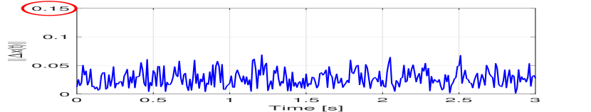
(a) System without attack

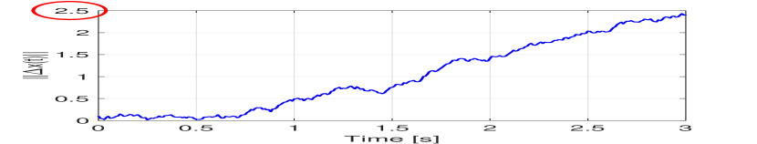
(b) Under a perfect attack, without authentication

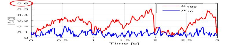
(c) With two different integrity enforcement policies, with periods $L=10,100$

Figure 2: Evolution of the estimation error norm for the VTF system; note the highlighted (circled) different error ranges.

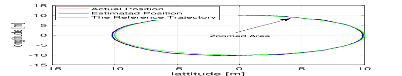
(a) State estimates under stealthy attack with integrity enforcement policy $L=10$.

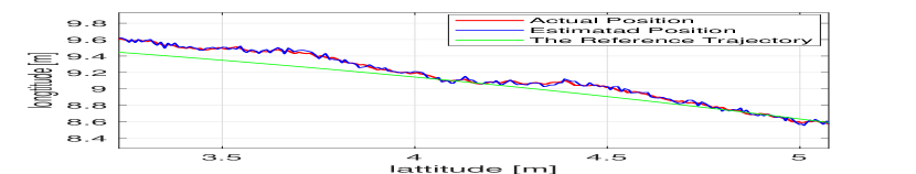
(b) Zoomed area of (a)

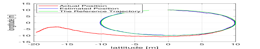
(c) State estimates under stealthy attack without integrity enforcement

Figure 3: Simultaneous trajectory tracking and state estimation for the VTF system. At each time step, system state is estimated and used by the controller to track a circle trajectory. The duration of the simulation is $60~{}s$ and the attack starts at $t=20~{}s$.

6 Conclusion

In this work, we considered the problem of resilient state estimation for LTI systems with bounded noise, when a subset of sensors are under attack. We defined two notions of perfect attackability (PA) – at a time point and over time – where stealthy attacks can cause an arbitrarily large estimation errors, and derived necessary and sufficient conditions for PA. We showed that, unlike the Kalman filter-based observers, batch processing-based resilient state estimators (RSE), such as $l_{0}$-based RSE, may be perfectly attackable even if the plant is not unstable. Furthermore, we studied the effects of intermittent data authentication on attack-induced estimation error. We showed that it is sufficient to even intermittently use data authentication, once every bounded time period, to ensure that a system is not perfectly attackable.

References

- Fawzi et al. [2014] H. Fawzi, P. Tabuada, and S. Diggavi. Secure estimation and control for cyber-physical systems under adversarial attacks. IEEE Transactions on Automatic control, 59(6):1454–1467, 2014.
- Golub and Van Loan [2012] G. H. Golub and C. F. Van Loan. Matrix computations, volume 3. JHU press, 2012.
- Jovanov and Pajic [2019] I. Jovanov and M. Pajic. Relaxing integrity requirements for attack-resilient cyber-physical systems. IEEE Transactions on Automatic Control, 64(12):4843–4858, 2019. ISSN 2334-3303.
- Kerns et al. [2014] A. J. Kerns, D. P. Shepard, J. A. Bhatti, and T. E. Humphreys. Unmanned aircraft capture and control via gps spoofing. Journal of Field Robotics, 31(4):617–636, 2014.
- Khazraei and Pajic [2020] A. Khazraei and M. Pajic. Perfect attackability of linear dynamical systems with bounded noise. In 2020 American Control Conference (ACC), 2020.
- Khazraei et al. [2017] A. Khazraei, H. Kebriaei, and F. R. Salmasi. A new watermarking approach for replay attack detection in lqg systems. In 56th IEEE Annual Conf. on Decision and Control (CDC), pages 5143–5148, 2017.
- Kwon et al. [2014] C. Kwon, W. Liu, and I. Hwang. Analysis and design of stealthy cyber attacks on unmanned aerial systems. Journal of Aerospace Information Systems, 11(8):525–539, 2014.
- Langner [2011] R. Langner. Stuxnet: Dissecting a cyberwarfare weapon. IEEE Security & Privacy, 9(3):49–51, 2011.
- Lesi et al. [2017] V. Lesi, I. Jovanov, and M. Pajic. Security-aware scheduling of embedded control tasks. ACM Trans. Embed. Comput. Syst., 16(5s):188:1–188:21, 2017.
- Lesi et al. [2020] V. Lesi, I. Jovanov, and M. Pajic. Integrating security in resource-constrained cyber-physical systems. ACM Trans. on Cyber-Physical Systems, 2020. https://arxiv.org/abs/1811.03538.
- Luo et al. [2019] X. Luo, M. Pajic, and M. M. Zavlanos. A scalable and optimal graph-search method for secure state estimation. arXiv preprint arXiv:1903.10620, 2019.
- Mo and Sinopoli [2009] Y. Mo and B. Sinopoli. Secure control against replay attacks. In 47th Annual Allerton Conference on Communication, Control, and Computing, pages 911–918. IEEE, 2009.
- Pajic et al. [2014] M. Pajic, J. Weimer, N. Bezzo, P. Tabuada, O. Sokolsky, I. Lee, and G. Pappas. Robustness of attack-resilient state estimators. In ACM/IEEE International Conference on Cyber-Physical Systems (ICCPS), pages 163–174, April 2014.
- Pajic et al. [2017a] M. Pajic, I. Lee, and G. J. Pappas. Attack-resilient state estimation for noisy dynamical systems. IEEE Transactions on Control of Network Systems, 4(1):82–92, 2017a.
- Pajic et al. [2017b] M. Pajic, J. Weimer, N. Bezzo, O. Sokolsky, G. J. Pappas, and I. Lee. Design and implementation of attack-resilient cyberphysical systems: With a focus on attack-resilient state estimators. IEEE Control Systems Magazine, 37(2):66–81, 2017b.
- Pasqualetti et al. [2013] F. Pasqualetti, F. Dörfler, and F. Bullo. Attack detection and identification in cyber-physical systems. IEEE Transactions on Automatic Control, 58(11):2715–2729, 2013.
- Shoukry and Tabuada [2016] Y. Shoukry and P. Tabuada. Event-triggered state observers for sparse sensor noise/attacks. IEEE Trans. on Aut. Control, 61(8):2079–2091, 2016.
- Shoukry et al. [2017] Y. Shoukry, P. Nuzzo, A. Puggelli, A. L. Sangiovanni-Vincentelli, S. A. Seshia, and P. Tabuada. Secure state estimation for cyber-physical systems under sensor attacks: A satisfiability modulo theory approach. IEEE Transactions on Automatic Control, 62(10):4917–4932, 2017.
- Smith [2015] R. S. Smith. Covert misappropriation of networked control systems: Presenting a feedback structure. IEEE Control Systems Magazine, 35(1):82–92, 2015.
- Sundaram and Hadjicostis [2011] S. Sundaram and C. N. Hadjicostis. Distributed function calculation via linear iterative strategies in the presence of malicious agents. IEEE Transactions on Automatic Control, 56(7):1495–1508, 2011.
- Sundaram et al. [2010] S. Sundaram, M. Pajic, C. Hadjicostis, R. Mangharam, and G. Pappas. The Wireless Control Network: Monitoring for Malicious Behavior. In 49th IEEE Conference on Decision and Control (CDC), pages 5979–5984, Dec 2010.
- Teixeira et al. [2012] A. Teixeira, D. Pérez, H. Sandberg, and K. H. Johansson. Attack models and scenarios for networked control systems. In 1st ACM Int. Conf. on High Confidence Netw. Systems, pages 55–64, 2012.
- Teixeira et al. [2015] A. Teixeira, I. Shames, H. Sandberg, and K. H. Johansson. A secure control framework for resource-limited adversaries. Automatica, 51:135–148, 2015.
- Y. Mo and B. Sinopoli [2010] Y. Mo and B. Sinopoli. False data injection attacks in control systems. In First workshop on Secure Control Systems, pages 1–6, 2010.
- Zetter [2016] K. Zetter. Inside the cunning, unprecedented hack of ukraine’s power grid. Wired, 2016.