Analytic Signal Phase in $\mathop{N\mathchar 45\relax D}$ by Linear Symmetry Tensor–fingerprint modeling

Abstract

We reveal that the Analytic Signal phase, and its gradient have a hitherto unstudied discontinuity in $\mathop{2\mathchar 45\relax D}$ and higher dimensions. The shortcoming can result in severe artifacts whereas the problem does not exist in $\mathop{1\mathchar 45\relax D}$ signals. Direct use of Gabor phase, or its gradient, in computer vision and biometric recognition e.g., as done in influential studies [12, 36], may produce undesired results that will go unnoticed unless special images similar to ours reveal them. Instead of the Analytic Signal phase, we suggest the use of Linear Symmetry phase, relying on more than one set of Gabor filters, but with a negligible computational add-on, as a remedy. Gradient magnitudes of this phase are continuous in contrast to that of the analytic signal whereas continuity of the gradient direction of the phase is guaranteed if Linear Symmetry Tensor replaces gradient vector. The suggested phase has also a built-in automatic scale estimator, useful for robust detection of patterns by multi-scale processing. We show crucial concepts on synthesized fingerprint images, where ground truth regarding instantaneous frequency, (scale & direction), and phase are known with favorable results. A comparison to a baseline alternative is also reported. To that end, a novel multi-scale minutia model where location, direction, and scale of minutia parameters are steerable, without creation of uncontrollable minutia is also presented. This is a useful tool, to reduce development times of minutia detection methods with explainable behavior. A revealed consequence is that minutia directions are not determined by the linear phase alone, but also by each other and the influence must be corrected to obtain steerability and accurate ground truths. Essential conclusions are readily transferable to $\mathop{N\mathchar 45\relax D}$, and unrelated applications, e.g. optical flow or disparity estimation in stereo.

1 Introduction

Phase is extensively used in speaker and speech recognition [31], Geo and seismic studies [9][25], as well as in optics [2]. It is also used in biometric identification and image processing since long, [36], [18], [17]. Inspired by $\mathop{1\mathchar 45\relax D}$, and given the ill-posedness of continuous Phase unwrapping, one approach has been to use the derivative of phase e.g. [12], since the derivative is continuous in $\mathop{1\mathchar 45\relax D}$, even if the phase is not.

Analytic Signal concept originates in real functions of $\mathop{1\mathchar 45\relax D}$ where negative frequencies of a function are set to zero. The procedure does not yield a loss of information because a real signal $f(r)$, has the Fourier Transform $F(\omega)$, FT, with complex values containing redundant information: $F(\omega)=F^{*}(-\omega)$. This is also known as the Hermitian Symmetry. Thereby, the Analytic Signal is complex valued and has phase in its values.

The Analytic Signal, $z(\bm{r})$, corresponding to a real function $f(\bm{r})$ where $\bm{r}\in\mathop{N\mathchar 45\relax D}$ can be defined in a similar manner. Thus $z(\bm{r})$ corresponding to $f(\bm{r})$ is obtained by the inverse FT of $Z(\bm{\omega})=F\cdot\chi(\bm{\hat{n}}^{T}\bm{\omega})$ where $\chi$ is the Heaviside function, which assumes values zero or one.

A different extension of the analytic signal to $\mathop{2\mathchar 45\relax D}$ is offered via the Riesz transform. It assumes that the local input is linearly symmetric, [5], also known as intrinsically $\mathop{1\mathchar 45\relax D}$, and the direction of the symmetry is known. Then phase, direction and amplitude of the local input can be embedded in a $\mathop{3\mathchar 45\relax D}$ hypercomplex [10] field, called the monogenic signal. The three elements can be computed via convolutions by quadrature filters, yielding a linear feature vector, [11], [26], [33], tuned to a fixed scale. The resulting phase does not coincide with the FT phase if a dominant direction cannot be computed, [1]. By contrast, phase interpretation provided by narrow bandwidth Gabor filters coincides with that of the FT phase even if the input signal is not linearly symmetric. Nonetheless, the discontinuity of phase and its gradient, which we will detail in the sequel, cause similar artifacts in the phase of monogenic signal. A taxonomy of phase discontinuities is also a main motivation of the present study.

2 Analytic Signal by Gabor filtering

A Gabor filter is defined conveniently in the FT domain as a Gaussian located at $\bm{\omega}$. In the spatial domain, the filter is then given by

$$g_{\sigma^{2},\bm{\omega}_{k}}(\bm{r})\!=\!\frac{1}{c}\!\exp(i\bm{\omega}_{k}^{T}\!\bm{r})\!\exp(\!-\frac{\|\bm{r}\|^{2}}{2\sigma^{2}})$$ (1)

such that its magnitude is a Gaussian, with variance $\sigma^{2}$ where $c=(2\pi\sigma^{2})^{N/2}$ and $\bm{r},\bm{\omega}_{k}\in R^{N}$.

A Gabor filter response to a real (local) image $f$ is complex valued. It is obtained as a collection of scalar products with translated versions of $g$, typically obtained by convolution

$$\!z_{\bm{\omega}_{j}}(\bm{r})\! = \!\langle g_{\sigma^{2},\bm{\omega}_{j}}(\bm{r}-\bm{r}^{\prime})\,,f\rangle$$ (2)

$$= \int g_{\sigma^{2},\bm{\omega}_{j}}^{*}(\bm{r}-\bm{r}^{\prime})f(\bm{r}^{\prime})d\bm{r}^{\prime}$$

A collection of such responses obtained for a set of $\{\bm{\omega}_{j}\}$ at the same image location $\bm{r}$ represent the sampled local spectrum since filter bandwidths can be made appropriately small in every direction by choosing $\sigma^{2}$ accordingly, including by making $\sigma^{2}$ to depend on $\bm{\omega}_{j}$. Because of the latter, and to reduce symbol clutter, we have omitted to express dependency of $z$ on $\sigma^{2}$ in (2).

Gabor filters must be placed on the same side of an arbitrary but fixed hyper-plane passing through the spectral origin to provide a sampled version of the analytic signal. The normal of the hyper-plane, $\bm{\hat{n}}$, pointing into the non-zero half space and is called walking direction here.

2.1 Linear Symmetry Tensor driven phase $\Phi^{LS}$

Using the scalar product definition in (2), Linear Symmetry, LS, tensor $\bm{S}^{D}$ is obtained as an $N\times N$ matrix by convolutions combined with intermediate pixel-wise products, [5],

$$\bm{S}^{D}(\bm{r})=\langle\nabla f\,,\nabla^{T}f\rangle$$ (4)

LS tensor is generalizable to curvilinear coordinates defined by harmonic functions [3]. It can estimate local image direction $\bm{\omega}$, and $N$ coherence/certainty measures, representing the error between a component tensor model and the local image. This is also the reason why “D” (for intrinsic direction) marks the tensor in the equation. The concept of direction comprises direction in local harmonic curves which can define intricate symmetries. Coherence measures are obtained by eigenvalues of the LS tensor whereas eigenvectors represent tensor model parameters (the directions) explaining the input data best.

The eigenvalue decomposition of the tensor can be rearranged further to represent subspaces pedagogically, especially in its Cartesian $\mathop{N\mathchar 45\relax D}$ generalization, e.g. as a linear combination of the “plane” tensor, “stick” tensor, “ball” tensor etc, [20], [29], [4]. A $\mathop{2\mathchar 45\relax D}$ version of the LS tensor without generalizations (to $\mathop{N\mathchar 45\relax D}$ nor to harmonic functions) was simultaneously suggested in [21]. Its eigenvalue combinations were suggested early as corner detectors, [14], [19]. LS tensor is also known as Structure Tensor [23], and can be estimated by quadrature filters.

In a recent result on LS tensor, it has been shown that the trace of the tensor in the log-scale space yields another LS tensor, $\bm{S}^{S}$. The latter is always a $2\times 2$ matrix, regardless the “$N$”. The tensor $\bm{S}^{S}$ determines the characteristic absolute frequency of the local image, $\|\bm{\omega}\|$, where “$S$” in the exponent marks that it is an LS tensor representing the intrinsic scale. The absolute frequency is also known as scale as both are terms used to represent the intrinsic “size” associated with a pattern. Thereby scale is determined by eigenvectors of $\bm{S}^{S}$ whereas coherence w.r.t. scale is determined by its eigenvalues, [6]. Thus, using $\bm{S}^{D}$ for direction and $\bm{S}^{S}$ for scale, $\bm{\omega}$ and up to $N+2$ coherence measures ($N$ for direction and $2$ for the scale) can be obtained. We recall that without help of $\bm{S}^{S}$, one can only estimate the direction of $\bm{\omega}$ by $\bm{S}^{D}$, up to a sign change i.e. $\pm\bm{\omega}/\|\bm{\omega}\|$.

LS tensor driven phase, $\Phi^{LS}$, is the phase of

$$z_{\bm{\omega}(f)}(\bm{r})\!=\!u(\bm{r})\!+\!iv(\bm{r})\!=\!m(\bm{r})\!\exp(i\Phi^{LS}(\bm{r}))$$ (5)

which is the response of a Gabor filter tuned to $\bm{\omega}$ estimated via $\bm{S}^{D}$, and $\bm{S}^{S}$ i.e.

$$\Phi^{LS}(\bm{r})=\arg(z_{\bm{\omega}(f)}(\bm{r}))$$ (6)

Here $f$ is the input image, and the $\bm{\omega}(f)$ in $z_{\bm{\omega}(f)}$ is the tune-in frequency vector estimated by $\bm{S}^{D}$, and $\bm{S}^{S}$. Dependence of this phase on the walking direction $\bm{\hat{n}}$ is implicit, as our analytic signal in $\mathop{N\mathchar 45\relax D}$ is the classic one, presupposing an arbitrary (but fixed) $\bm{\hat{n}}$. LS tensor driven phase necessitates $\bm{\omega}(r)$ along with coherence measures, allowing to determine where in the image $\bm{\omega}$ is meaningful to compute.

2.2 Comparison of phase in $\mathop{1\mathchar 45\relax D}$ and $\mathop{N\mathchar 45\relax D}$

Gradient field of the phase, $\nabla\Phi^{LS}(\bm{r})$, defines the instantaneous frequency (vector field). A sinusoid $f$ is the motivating example of the definition, where the gradient “kicks-out” the frequency vector.

$$f=\cos({\bm{\omega}^{T}\!\bm{r}})\;\;\Leftrightarrow\;\;z=\exp(i\bm{\omega}^{T}\!\bm{r})\;\;\bm{r},\bm{\omega}\in R^{N}$$ (7)

The complex version of the sinusoid, $z$, is the illustrious example of the analytic signal. Here, the challenge is to define a useful phase in $\mathop{N\mathchar 45\relax D}$. It is a challenge because for such a sinusoid there exists singular directions at every location $\bm{r}$ along which one can translate (“walk in”) the local signal, and yet the phase of $z$ remains unchanged. Singular directions (denoted by $\bm{\omega}_{\perp}$) are given by the $N-1$ dimensional subspace containing vectors orthogonal to $\bm{\omega}$, that is $\bm{\omega}_{\perp}^{T}\bm{\omega}=0$. By contrast, in $\mathop{1\mathchar 45\relax D}$, i.e. $\bm{r}=r\in R^{1}$, there is a change of phase as soon as location changes. For this reason, in $\mathop{1\mathchar 45\relax D}$, the location $r$ relative to a landmark can be uniquely determined, from the phase of $z$ (though up to period $2\pi/\omega$) but not in $\mathop{N\mathchar 45\relax D}$. Directions, including singular directions, do not exist in $\mathop{1\mathchar 45\relax D}$.

To recover $\bm{r}\in R^{N}$ by phase of $z(\bm{r})$ is impossible for dimensions $N>1$. The next best thing to achieve is a projection of $\bm{r}$ on the direction of the wavefront of the sinusoid, $\bm{\omega}$. In turn this requires that $\bm{\omega}$, including its norm, is reliably estimated so that a phase change can be mapped to a displacement of $\bm{r}$ in the direction of $\bm{\omega}$, up to period $2\pi/\|\bm{\omega}\|$. Accordingly, availability of $\bm{\omega}$ estimation, is a sine-qua-non of a phase estimation in $\mathop{N\mathchar 45\relax D}$.

Another difference of $\mathop{N\mathchar 45\relax D}$ in comparison to $\mathop{1\mathchar 45\relax D}$ is that the Analytic Signal $z(\bm{r})$ is not unique since $\bm{\hat{n}}$, defining half the volume of FT domain, is not unique. The half volume can be chosen arbitrarily via $\bm{\hat{n}}$.

2.3 Modeling, synthesizing and controlling minutiae by phase

Often, high quality is a challenge or impossible to obtain when imaging fingerprints, e.g. of crime scenes [35]. One goal of this study is to contribute with automatic production of large numbers of images which have realistic appearance of local fingerprints. These are characterized by ridges changing direction, dotted with singularities representing ridge-ends or bifurcations, called minutiae, [22]. Minutiae are by far the most common features extracted and used for identification of fingerprints in Automated Fingerprint Identification Systems, AFIS, of law enforcement, in courts to convince judges, in convenient applications e.g. laptops, mobile phones and doors. Labeled minutiae are needed by the current pattern recognition trend, increasingly using deep neural networks, which require large data sets with known and steerable ground truths.

Labeled minutiae are also needed if minutiae detection algorithms are to be evaluated on their own merits, [30], disjoint from minutia matching algorithms. This can be done by using expert annotations. However, this is an expensive method beside that the variability is not sufficient, e.g. currently the only publicly available labeled minutia data-set, [15], contains around 5500 minutiae pairs and contains fingerprints of adults only.

One problem in automatic synthesis of minutiae is steerability of ground truths, i.e. when minutiae are created in desired locations, new non-steerable and unavoidable minutiae can also be created. As will be discussed below, all minutiae also influence each other, which exacerbates the problem. Controllability of minutia presence and steerability of their properties when present have not been discussed in previous studies, [8], [7], but exists when attempting to create multiple minutiae, e.g. for automatic labeling.

In addition to ground-truths for traditional minutia properties, being location, direction, and type, we want that a new minutia property, absolute frequency, will be steerable too. We also want to control the amount and the nature of contamination/noise degrading minutiae quality. As will be shown below, minutia directions are not determined entirely by the global direction map. Even minutiae influences the final direction map, much like planets in the solar system influence the sun’s and each other’s gravitation fields.

The studies [32], [27] have recognized the importance of orientation maps, which can be obtained from LS tensor fields, [5], in localization and description of minutiae by searching for signatures in the gradient field of phase. An advantage of phase based (single) minutia model, which we chose to extend to multiple steerable minutiae here, is that it offers a direct synthesis of a minutia, in addition to their localization and description.

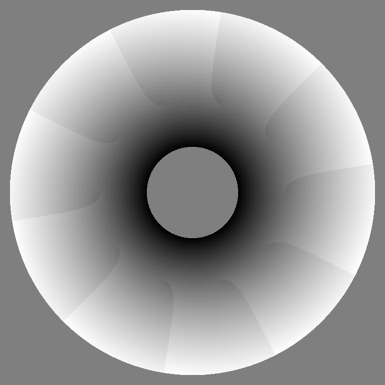
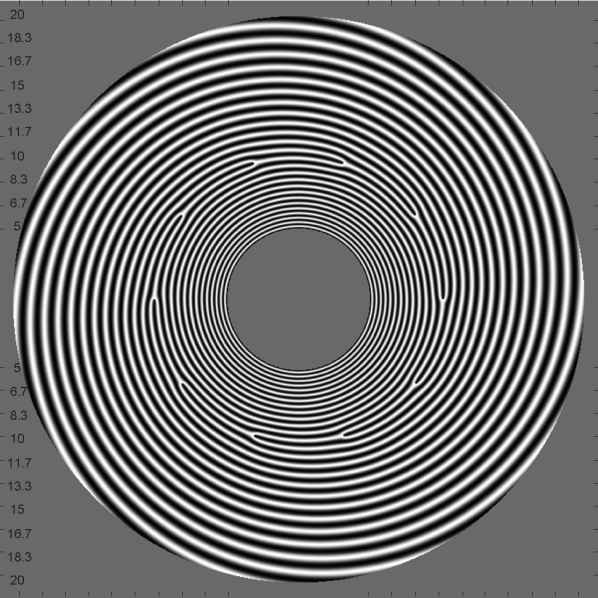
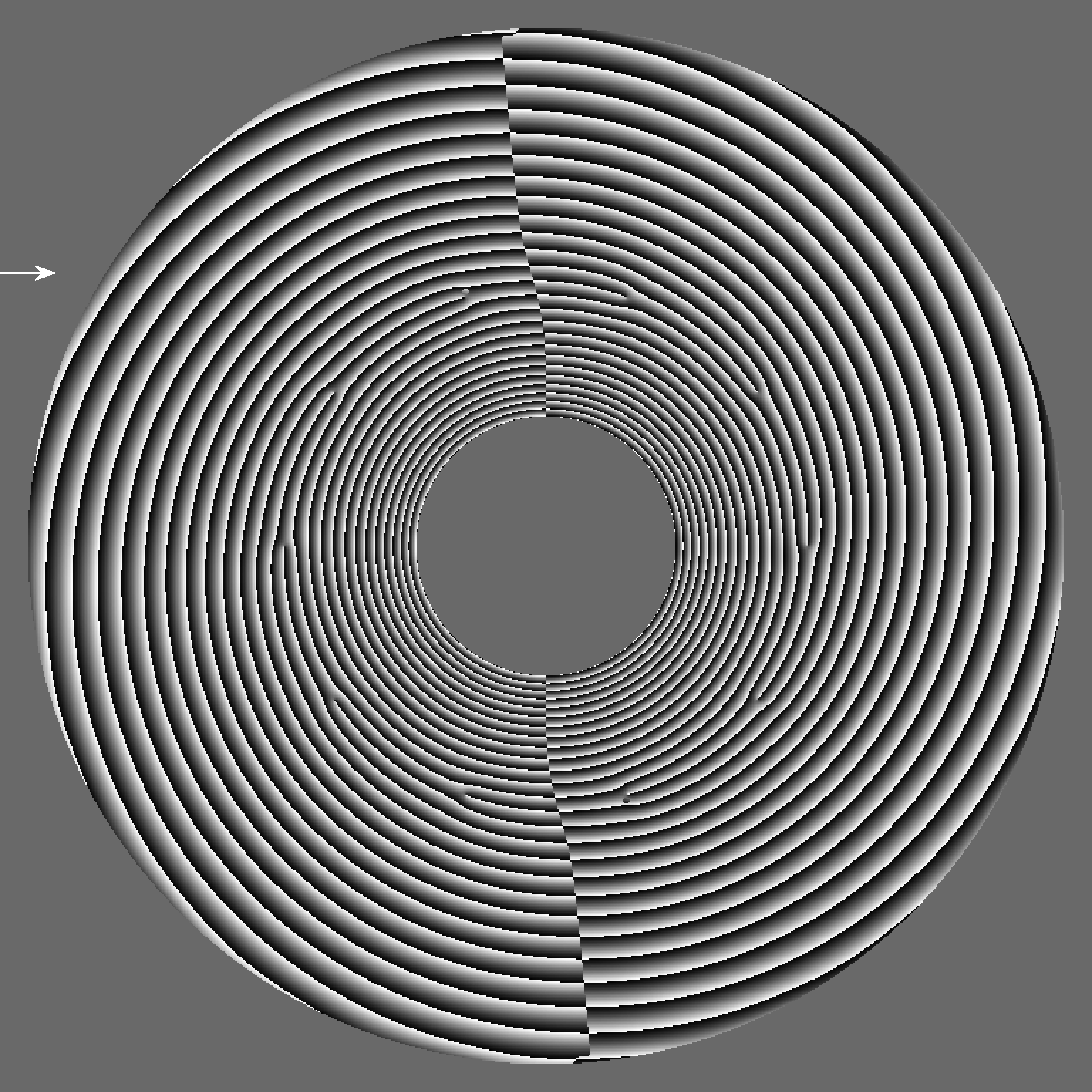
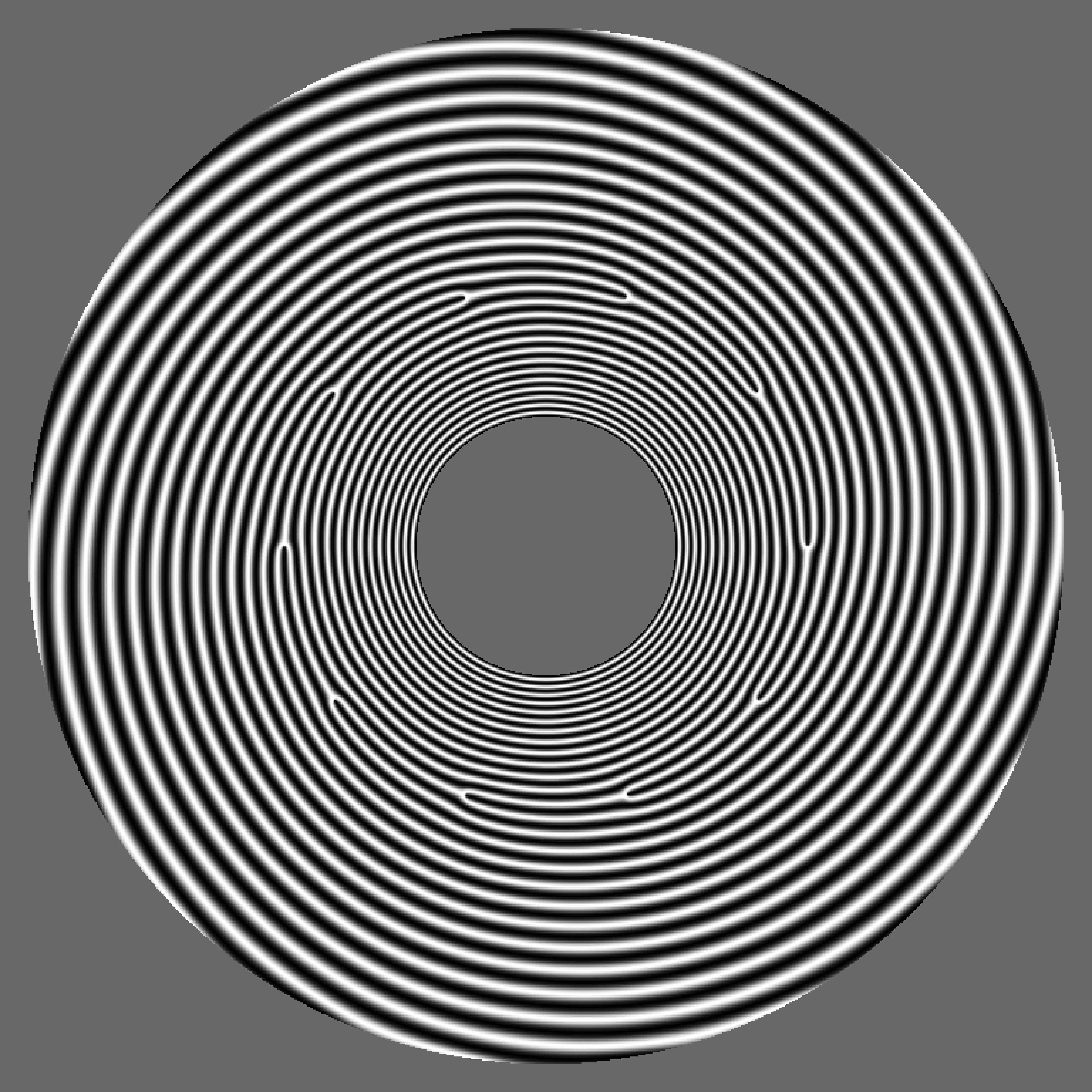
Figure 1: (L;R;T;D;) Continuous phase $\Phi$; Minutiae containing image $I$, produced by the continuous phase as $I=\Re\exp(i\Phi)$; LS tensor driven phase $\Phi^{LS}(I)$ estimated from $I$; Reconstruction by using the estimated phase $\Phi^{LS}(I)$ in $\Re\exp(i\Phi^{LS})$.

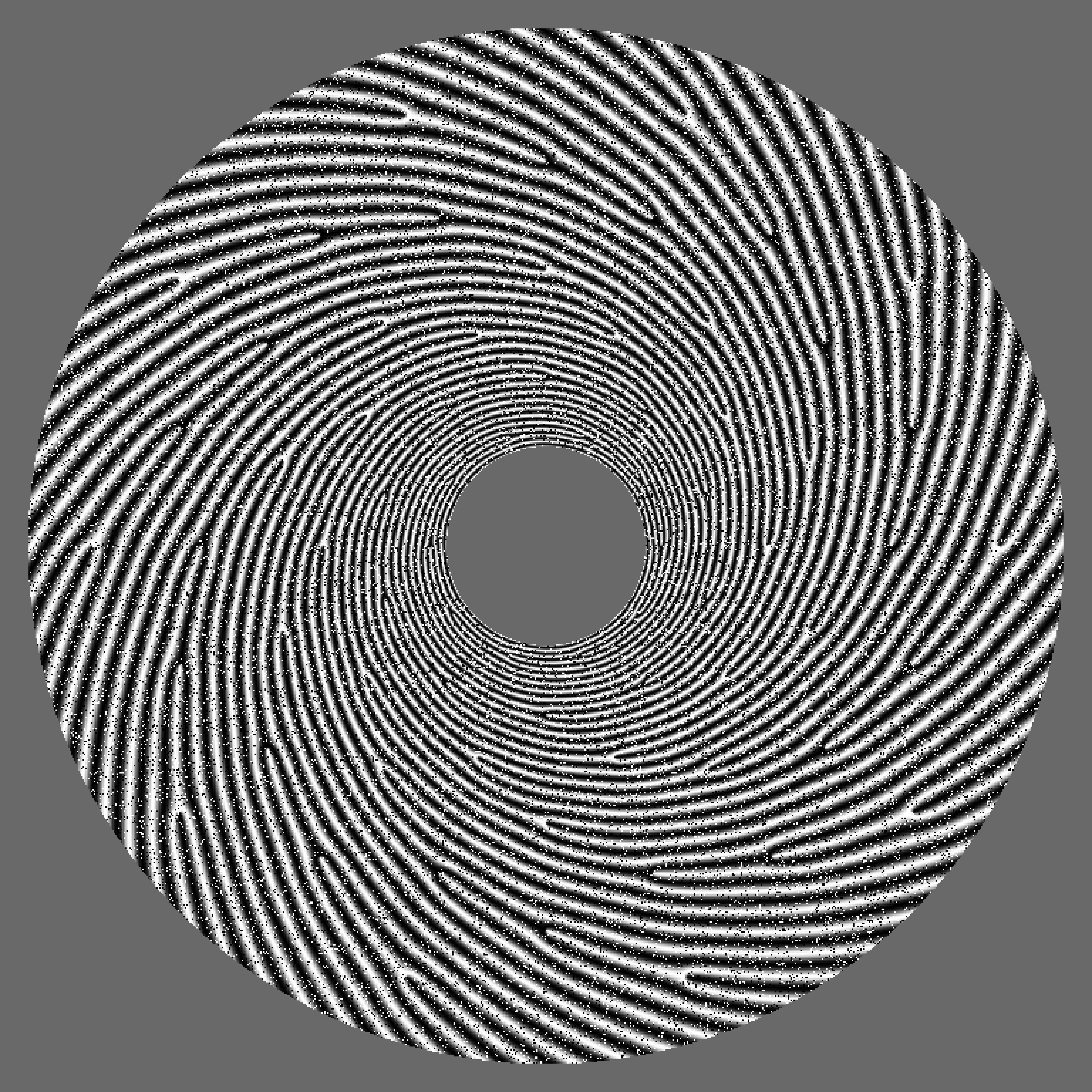
Figure 2: Minutiae are produced as in Fig. 3 but followed by contamination with noise. Ground-truths of minutia parameters, as well as phase, are the same.

In Fig. 1 (Top-R) a total of 10 minutiae all sharing the same type, bifurcation, and the same scale are shown, to serve as input with known ground-truth, to illustrate our point. Likewise, in Fig. 2, in total 70, both bifurcation and ridge-end minutia types are shown. Minutiae are embedded in waves whose instantaneous period, i.e. scale, changes continuously in a range which can be chosen. At four edges of Fig. 1 (Top-R) exact periods in mid vertical and horizontal directions have been indicated by ticks. Horizontal labels are not spelled out for compactness, but are deducable from vertical ones as they are identical. Random salt and pepper replacement, SPR, as shown in Fig. 2, or additive Gaussian noise (not shown) can be chosen to contaminate the image to simulate degradation of quality in a span of levels.

The degradation that we offer is basic and has the purpose to increase efficiency of developing novel algorithms with explainable behavior when variables of minutiae change. Explainability is a major weakness of Deep Learning networks, the performance of which depends on variability and statistics of training data, which is more efficiently controlled with synthetic data. The purpose of synthetic data is by no means to replace real data, but to make use of this precious data more efficiently.

To achieve this, we start with a single minutia model below, Eq. (8), and expand it to produce a constellation of minutiae in the same image. The model superposes a linear component and a non-linear component to produce the phase of a minutia:

$$\Phi(\bm{r})=\Phi_{L}(\bm{r})+\Phi_{P}(\bm{r})=\bm{\omega}^{T}\bm{r}+\arg(\frac{\tilde{\bm{r}}}{i\tilde{\bm{\omega}}})+(-1)^{t}\pi$$ (8)

where $\bm{\omega}$ is constant and $\bm{\omega},\bm{r}\in R^{2}$. The operator $\tilde{\cdot}$ turns the $\mathop{2\mathchar 45\relax D}$ vector in the place holder “$\cdot$”, to the corresponding complex number, e.g. if $\bm{r}=(1,1)^{T}$, then $\tilde{\bm{r}}=1+i$. The first term $\Phi_{L}(\bm{r})$, the linear phase, is responsible for generating the local planar wave of ridges, with $\bm{\omega}$ being its frequency vector. Later, the vector $\bm{\omega}$ will be allowed to change spatially slowly, so that in a small neighborhood it can be viewed as constant.

The second component $\Phi_{P}(\bm{r})$, called polar phase, (also known as spiral phase) produces a continuous phase increase (modulo $2\pi$) when moving around the origin, set to the current point in the equation to avoid symbol clutter. Dividing $\tilde{\bm{r}}$ with $i\tilde{\bm{\omega}}$ starts the increase from the iso-curve direction of the current (ridge) point. Addition of the two terms produces the phase of a minutia having the direction $\arg(i\tilde{\bm{\omega}})$, measured in the way ISO standard does, at a neighborhood having $|\tilde{\bm{\omega}}|$ as absolute frequency of the underlying planar wave.

The third term determines the type, where $t\in\{0,1\}$, switches between $\{\hbox{\em bifurcation},\hbox{\em ridge-end}\}$, respectively.

Other intermediate directions can be obtained by rotating the local coordinate frame, whereas scale can be changed to the desired one by changing $\|\bm{\omega}\|$. A local image, $I$, containing a minutia at the origin is then obtained by taking the real part of the complex wave having $\Phi$ as its phase,

$$I(\bm{r})=\Re(\exp(i\Phi(\bm{r})))$$ (9)

where iso-gray curves of $I$ are the same as those of $\Phi$.

For a desired set of minutiae with minutia $j$ at location $\bm{r}_{j}$, all sharing the same minutia type, one can synthesize a fingerprint image by the additive, polar phase model:

$$\Phi(\bm{r})\!\!\! = \!\!\!\Phi_{L}(\bm{r})+\Phi_{P}(\bm{r})$$ (10)

$$= \!\!\!\bm{r}^{T}\bm{\omega}^{L}\!(\bm{r})+(-1)^{t}\pi+\!\sum_{j}\!\arg(\frac{\tilde{\bm{r}}-\tilde{\bm{r}}_{j}}{i\tilde{\bm{\omega}}_{j}})$$

where $\bm{\omega}^{L}(\bm{r})$ is such that it varies slowly with $\bm{r}$ and can be assumed to be constant when $\bm{r}$ is near minutia location $\bm{r}_{j}$. When aggregated, minutiae have to be described relative the (common) origin rather than minutiae singularities, explaining translations with $\tilde{\bm{r}}_{j}$ depicting their locations. Also, the minutia direction must be parallel to the direction of the surrounding ridges, i.e. the minutia direction is orthogonal to the direction of the wave vector of the surrounding waves. This is achieved by the complex division with $i\tilde{\bm{\omega}}_{j}$.

In case $j$ is the only minutia in the image, both $\bm{\omega}^{L}(\bm{r}_{j})$ and $i\bm{\omega}_{j}$ directions agree because the polar phase is then alignable with linear phase by complex division with $i\tilde{\bm{\omega}}_{j}=i\tilde{\bm{\omega}}_{j}^{L}$, (10). However, they are generally different in case there are more than one minutia in the image. Phase of other minutiae, in addition to the linear phase will contribute to the phase in the vicinity of $\bm{r}_{j}$ which in turn will contribute to a change of $\bm{\omega}^{L}$. To find the resulting minutia direction, we apply $\nabla$ to (10). The left hand side is then the instantaneous wave vector, $\bm{\omega}(\bm{r})=\nabla\Phi(\bm{r})$. The right hand side is composed by the gradient of the linear term and aggregated gradients of polar terms of all minutiae.

$$\bm{\omega}(\bm{r}) = \nabla\Phi_{L}+\sum_{k}\nabla\arg(\frac{\tilde{\bm{r}}-\tilde{\bm{r}}_{k}}{i\tilde{\bm{\omega}}_{k}})$$ (11)

$$= \bm{\omega}^{L}(\bm{r})+\sum_{k}i\frac{\tilde{\bm{r}}-\tilde{\bm{r}}_{k}}{|\tilde{\bm{r}}-\tilde{\bm{r}}_{k}|^{2}}$$ (12)

To obtain (11), we have used the assumption that the linear phase varies slowly, i.e it is approximated well locally by $\Phi_{L}=\bm{r}^{T}\bm{\omega}^{L}$. Accordingly, the gradient of the linear term is yields $\nabla\Phi_{L}=\bm{\omega}^{L}(\bm{r})$. The result (12) yields noting that gradient fields of polar phases are additive and, that the factor $1/i\tilde{\bm{\omega}}_{k}$ does not influence such gradient contributions. The latter is because such factors subtract (constant) start angles which disappear under derivation. Thus, the above equation can be sampled at $\bm{r}_{j}$, wherein $\bm{\omega}^{L}$ is replaced with $\bm{\omega}^{L}_{j}$ and $\bm{r}$ is replaced with $\bm{r}_{j}$. The last term in the equation changes as $1/\|\bm{r}\|$ in local minutia coordinates, proving that the global direction map, $\nabla\Phi_{L}$, is corrected by individual minutiae in a similar manner as the gravitation field of the sun is corrected by contributions from all masses of planets.

In a real fingerprint, ground-truth w.r.t. slowly varying $\Phi_{L}$ and its directions are unknown, in addition to those of minutiae. Determination of ground-truths, if needed is possible by experts but it is very costly. This is another motivation of the present study, namely to construct synthetic test images which will mimic real fingerprints with precisely known ground-truths even w.r.t. $\Phi_{L}$ and its directions which must accord with minutia directions.

In particular, for the image shown in Fig. 1 (Top-L) which represents the continuous phase $\Phi$, we have selected

$$\Phi_{L}(\bm{r})=C\log(\|\bm{r}\|)$$ (13)

as slowly varying linear phase, as its symmetry eases visual evaluations too. Here, the coordinate origin is the center of the image and $C$ is a constant. The image represents the continuous phase $\Phi=\Phi_{L}+\Phi_{P}$. Thus it contains the polar phase superimposed on the linear one. Without the term $\Phi_{P}$, the phase $\Phi$ would be perfectly rotationally symmetric, i.e. $\Phi(\|\bm{r}\|)$, which it is not due to minutiae produced via $\Phi_{P}$ breaking the symmetry. The 10 Polar phase locations are clearly visible.

To compute $\Phi$ one needs to determine $\bm{\omega}_{j}$ at every polar phase (minutia) location. We have done this via $\bm{\omega}_{j}=\nabla\Phi(\bm{r}_{j})$ using (12).

$$\bm{\omega}_{j}=\bm{\omega}(\bm{r}_{j})=C\frac{\bm{r}_{j}}{\|\bm{r}_{j}\|^{2}}+\sum_{k}i\frac{\tilde{\bm{r}}_{j}-\tilde{\bm{r}}_{k}}{|\tilde{\bm{r}}-\tilde{\bm{r}}_{k}|^{2}}$$ (14)

where we have applied the fact that $\nabla\Phi_{L}=C\frac{\bm{r}}{\|\bm{r}_{j}\|^{2}}$.

The constant $C$ in (13) is the means to control the range of scales appearing in the image. By way of example, the constant C is determined by assuming that there are no-minutia in the image. The scale can be formally defined as $T$ which is $2\pi/\|\bm{\omega}\|$. The absolute frequency $\|\bm{\omega}\|$, is obtained by applying gradient to (13), yielding $\|\bm{\omega}\|=\frac{C}{\|\bm{r}\|}$. Accordingly, $C=2\pi\|\bm{r}_{\max}\|/T_{\max}$ is fixated by means of the largest allowed scale of planar waves, $T_{\max}$, which is attained at locations with largest radius, $\|\bm{r}_{\max}\|$. In turn this determines the image size. The tiniest allowed scale $T_{\min}$ determines likewise the inner radius of the test image $\bm{r}_{\min}$ via $\frac{2\pi}{T_{\min}}=\frac{C}{\|\bm{r}\|}$, within which the image is set to a constant.

Next, we design minutiae at desired scale and locations. Plugging (14), (13) into (10) yields $\Phi$, e.g. Fig. 1 (Top-L). In turn this produces via (9) the corresponding minutia image. Fig. 1 (Top-R), containing 10 minutiae sharing the same scale is obtained in this manner from Fig. 1 (Top-L). It is evident from the result that multiple minutia presence in the same scale has caused a correction to direction resulting in a spiral pattern. Without minutia, the monotonously increasing linear phase in radial direction would produce perfect circles.

Likewise, Fig. 2 containing 7 different scales with 10 minutiae in each with regularly alternating type, was obtained in an analogous manner. The evidence of spirals is more prominent suggesting that the more minutia there are the more they influence each other’s minutia directions. Each minutia corrects the direction of the linear phase as well as directions of other minutia in our model. To the best of our knowledge, a multi minutia model, (10), (12), explaining and computing the influence of minutiae on each other’s direction as well as on the global direction map explicitly is a novelty.

Contamination was applied after the minutia image was synthesized by replacing pixels randomly with black or white, Salt & Pepper Replacement, SPR, noise. To keep the study focused, we do not dwell on other degradations, which are evidently possible.

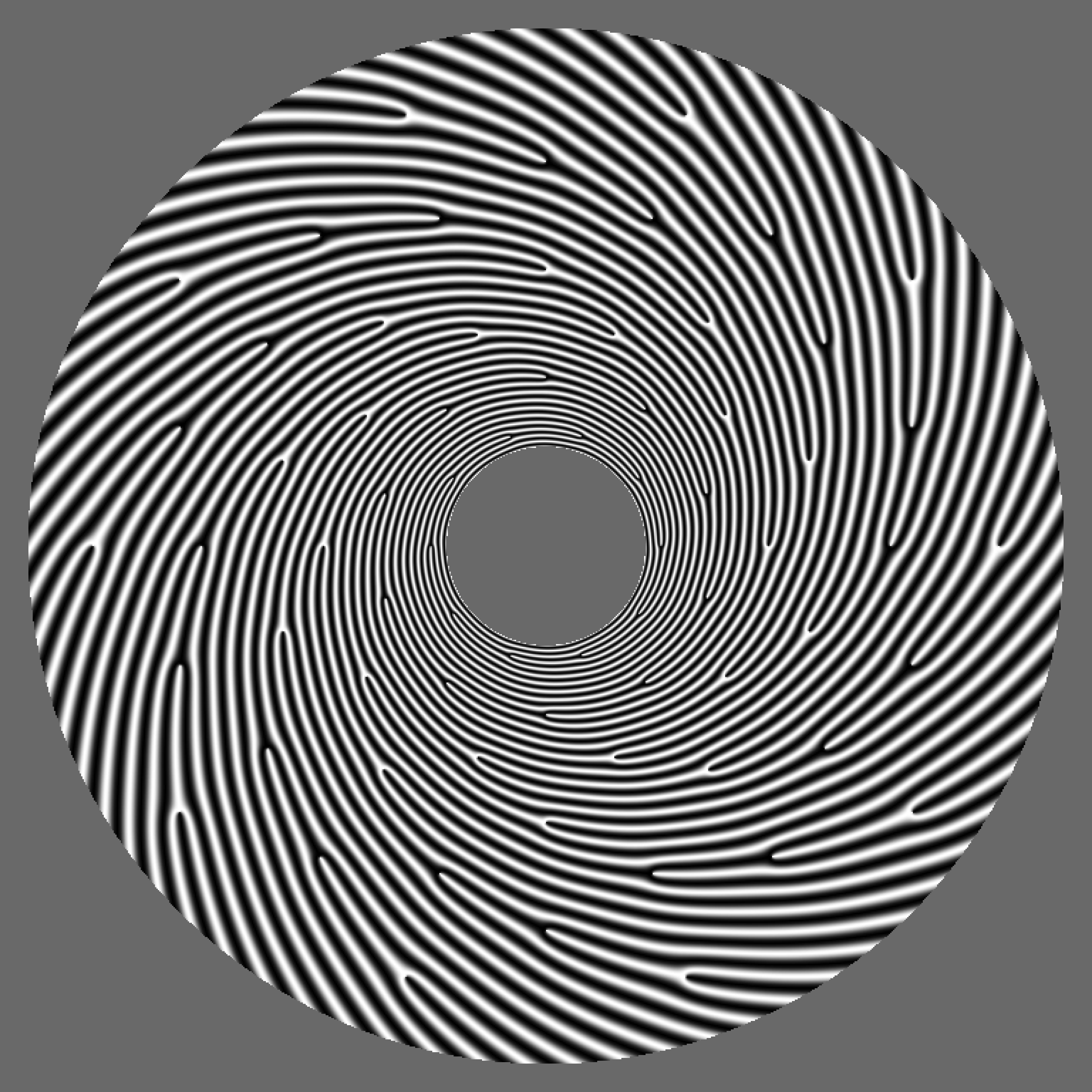
Figure 3: Seven Scales of 70 minutiae with different directions and periods. Minutiae are produced by the synthesis of $\Phi$. Ground-truths of minutia parameters, as well as phase, are known.

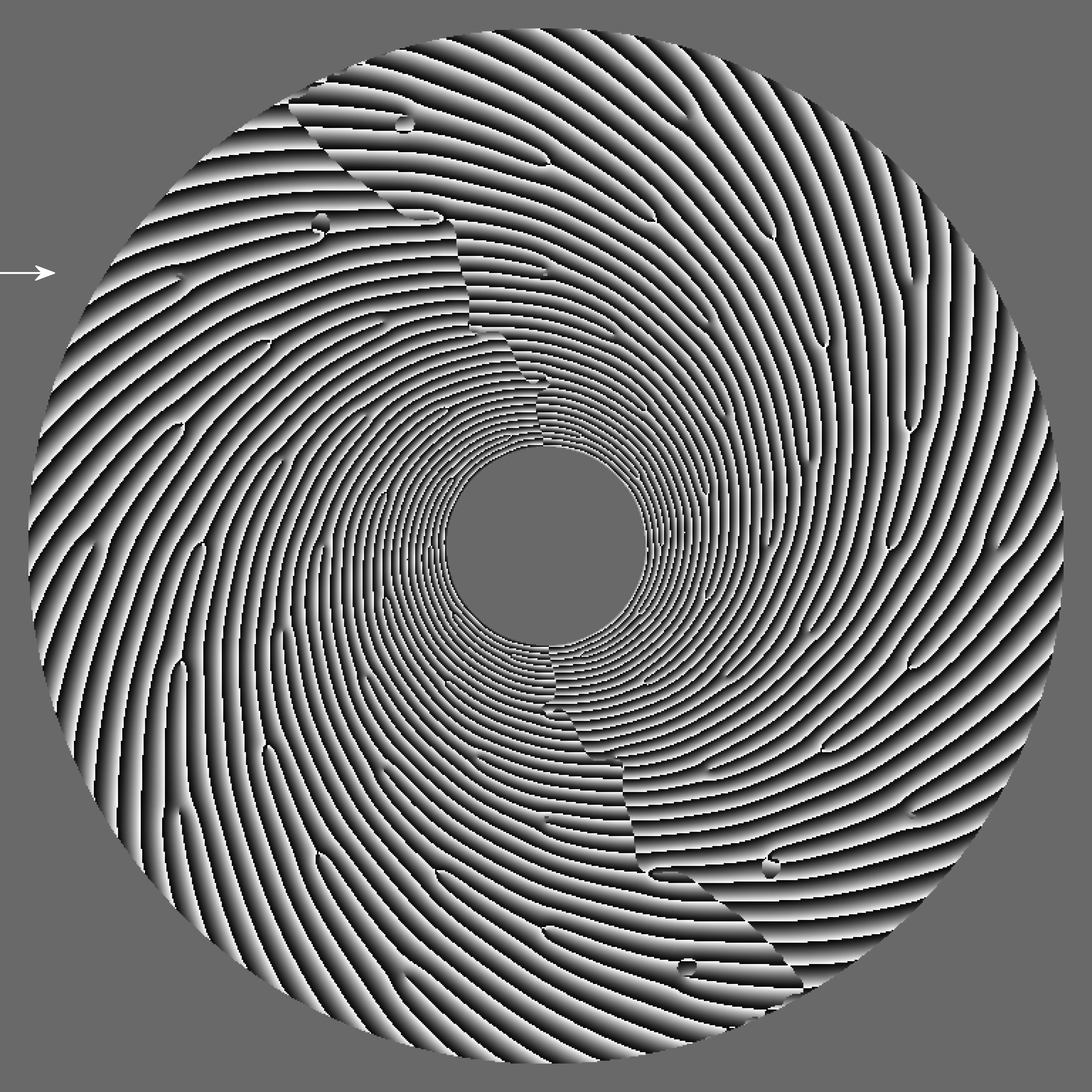
Figure 4: LS tensor driven phase of Fig. 3;

3 Artifact discontinuities of phase and noise

Fig. 1 (Top-R) and Fig. 3 show synthetic images containing fingerprint minutiae obtained by phase obtained via (14). Fig. 1 (Down-L) shows the LS tensor driven phase. Likewise Fig. 4 shows the LS tensor driven phase, on Fig. 3 to depict artifacts. We distinguish two types of artifacts in the phase, discussed next.

3.1 Circular discontinuities

Figure 1 (Down-L) shows LS tensor driven phase $\Phi^{LS}$ of the image $I$ (Top-R) computed via (6). Radially, gray values in $\Phi^{LS}$ have saw-toothed shape since the computed phase is only piece-wise linear instead of being fully linear w.r.t. $\bm{r}$. This is because angles constitute an equivalence class under addition of $2\pi k$, with $k$ being (unknown) integer, and computations involved in $\Phi^{LS}$ are local. Computed phase $\hat{\phi}$ is therefore not equal to the continuous phase $\Phi$ (Top-L). The discontinuities, along radial directions have jumps of exactly $2\pi$ and are called here circular discontinuities. They disappear if one enforces modulo $2\pi$ equivalence of $\Phi^{LS}$. For example, if we would have used HSV color representation (instead of gray levels) where the equivalence is present, such discontinuities would not be perceivable to human vision, Fig. 18 . Likewise, in machine vision, if we map the computed phase to e.g. $\exp(i\Phi^{LS})$, there Will be no such discontinuities after the mapping. This type of discontinuity appears in $\mathop{1\mathchar 45\relax D}$ as well as in higher dimensional signals. Circular discontinuity is the well-known phase unwrapping discontinuity, where phase jumps equal to (integer multiples of) $2\pi$. These are also visible in Fig. 4.

The extensively studied “phase unwrapping” problem e.g. in Synthetic Array Radar, SAR, imaging [16], aims at reconstructing continuous phase from wrapped phase. Solutions of the ill-posed problem fill circular discontinuities to yield as continuous a phase as possible. Gap constancy ($=2\pi$) at phase discontinuities is an overriding key assumption of algorithms suggesting solutions.

3.2 Hyper-Plane discontinuities

The second type is visible near the mid-column of Fig. 1 (Down-L), on waves with vertical wave vectors. It is due to $\bm{\hat{n}}$ and the local wave vector $\bm{\omega}$ is orthogonal to $\bm{\hat{n}}=0$. At such a point’s vicinity, $\bm{\omega}$ will wander in or out of the zero zone in the FT domain when $\bm{r}$ changes.

By construction, the phase must grow along the walking direction in a Gabor decomposition. This is evidenced by Fig. 1 (Down-L) where in the middle there is a jump but $\Phi^{LS}$ increases on both sides. The continuous phase (Top-L) obviously does not have jumps.

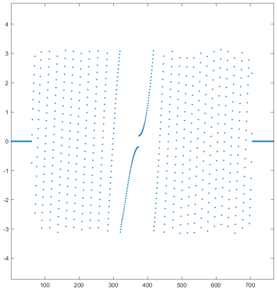
Figure 5: LS tensor driven phase along the white marked vector showing circular (saw-toothed) and hyper-plane (middle) discontinuities in Fig. 1 (D;L; White vector).

Such discontinuities are characterized by that i) they occur only at $\bm{r}$ where $\bm{\omega}(\bm{r})$ is orthogonal to the walking direction, $\bm{\omega}^{T}\bm{\hat{n}}=0$, ii) they occur only in $\mathop{N\mathchar 45\relax D}$ with $N>1$ since only then there is a direction concept at all for hyper-planes, iii) they disappear in representations where $\pm\bm{\omega}$ are equivalent. iv) discontinuity gaps equal to $2|\bm{\omega}^{T}\bm{r}|$ i.e. they depend on $\bm{r}$, The latter point is illustrated by comparing the gap at the central portion of Fig. 5 with $2\pi$ gaps. The graph is a snapshot of LS tensor driven phase image in the walking direction (white vector) of Figure 1 D;L. Accordingly, these artifact discontinuities are called here hyper-plane discontinuities. Hyper-Plane refers to the $N-1$ dimensional (arbitrary) hyper-plane separating the zero half from the non-zero half in the FT domain in which the Gabor decomposition has been defined.

The representation

$$I=\Re\exp(i\Phi^{LS})$$ (15)

is invariant to $\pm\Phi^{LS}$, thus invariant to $\pm\bm{\omega}$ when the phase is approximated well by linear phase, as well as full rotations $\Phi^{LS}+2\pi k$. These properties of the transformation are useful to avoid both artifact discontinuities. In (15), there is the implicit assumption that the local amplitude is known, and is set to 1. This is justified since our goal is to study the phase and normalizing local amplitude is one way to study the phase in isolation. Amplitude estimation can be done separately, e.g. by the magnitude $|z_{\bm{\omega}(f)}|$ when computing the LS tensor driven phase, (6).

Hyper-Plane artifacts are on continuous curves in $\mathop{2\mathchar 45\relax D}$, on continuous surfaces in $3\mathchar 45\relax D$, and generally on continuous $N-1$ dimensional planes embedded in $\mathop{N\mathchar 45\relax D}$ displaying non-constant phase jumps. Accordingly, a search for gaps of constant size as means to identify them, as is done in SAR phase unwarping, is bound to fail. Already in $\mathop{2\mathchar 45\relax D}$ images the loci of such points in LS tensor driven phase can be massive in length, e.g. in a fingerprint they can be continuous curves along which phase gradient have abrupt, unnatural direction changes, where phase jumps are not $2j\pi$.

Phase unwrapping algorithms, popular in SAR image processing, do attempt to remove artifact discontinuities, but the work hypothesis is that phase artifacts are due to circular discontinuities. One reason that this hypothesis makes sense in SAR context is that the phase comes from measured complex radar signals, phasors, as opposed to Gabor phase which is computed (from a real signal). Consequently, the FT of SAR (phasor) images are continuous whereas the reconstructed analytic signal has discontinuities in FT domain along a (randomly defined) hyper-plane. Thus it is a mistake to apply SAR phase unwrapping techniques to Gabor phase without taking into account hyper-plane discontinuities.

The need of an aggregated phase from phases of individual quadrature filters responses has been emphasized by [18], who also recognized their discontinuity in signs of edges in $\mathop{2\mathchar 45\relax D}$ images. However, to the best of our knowledge gaps of hyper-plane discontinuity in Gabor phase in $\mathop{N\mathchar 45\relax D}$, and remedies by using Gabor phase have not been identified and quantified before, although alternative phase representations have been suggested. On the contrary, phase of Gabor filter response has been used in feature vectors directly in numerous studies, e.g. in the influential study [36] in face recognition, without discussion of hyper-plane artifacts. Likewise, another influential study [12] in motion estimation, has relied on gradient of Gabor phase but fails short of identifying hyper-plane artifacts as obstacle. As detailed below, even phase gradients suffer from hyper-plane artifacts.

4 True discontinuities

True discontinuities correspond to abrupt changes in physical structures having expression in their images.

In $\mathop{2\mathchar 45\relax D}$ images, edges, corners, and line ends are such “visual objects”. In particular, minutia that will be discussed below, exemplifies true discontinuities in fingerprints.

Examples representing true discontinuities in higher dimensional images are blood vessel boundaries and junctions, tissue and organ boundaries, bone surfaces in tomography (volume) images, as well as boundaries of moving objects in video images.

Discontinuity in analytic signal phase in $\mathop{N\mathchar 45\relax D}$ is a hallmark of observations of true discontinuities, if one can discern them from artifact discontinuities. Using Gradient of Gabor phase is discussed next to model and detect true discontinuities, because it has been favored for the purpose by i) general $\mathop{N\mathchar 45\relax D}$ signal processing of human vision, [24] ii) $\mathop{3\mathchar 45\relax D}$ Gabor phase processing in previous studies, [12] and ii) by phase unwarping of SAR images, [16].

5 Image reconstruction/enhancement

The transformation in (15) is also the basis of our image enhancement suggestion using LS tensor driven phase. Essentially, $\Phi^{LS}$ is estimated first, and then the transformation is applied to the estimated phase. Fig. 1 (Down-R) corresponds to $I$ obtained from (15). It shows the result of enhancement using LS tensor driven phase $\Phi^{LS}$ estimation only, i.e. Fig. 1 (Down-L), without access to continuous phase (Top-L). The Real part of the complex signal delivered by the LS tensor driven phase represents a simple reconstruction mechanism of the original. Despite this, and that the estimation of $\bm{\omega}$ via Linear Symmetry Tensor must have operated under non-ideal conditions in minutia regions, the enhancement result does not suffer from artifacts. Non-ideal conditions in minutiae regions exist for LS tensor computations because, such regions have significant spiral term contributions, (10), (8), making them less than ideal planar waves. These regions are strictly speaking not linearly symmetric, even without noise. In comparison, Fig. 1 (Top-R) is the original produced by Fig. 1 (Top-L). Reconstruction errors of Fig. 1 (Down-R) around minutiae, representing true discontinuities discussed next, are virtually imperceptible.

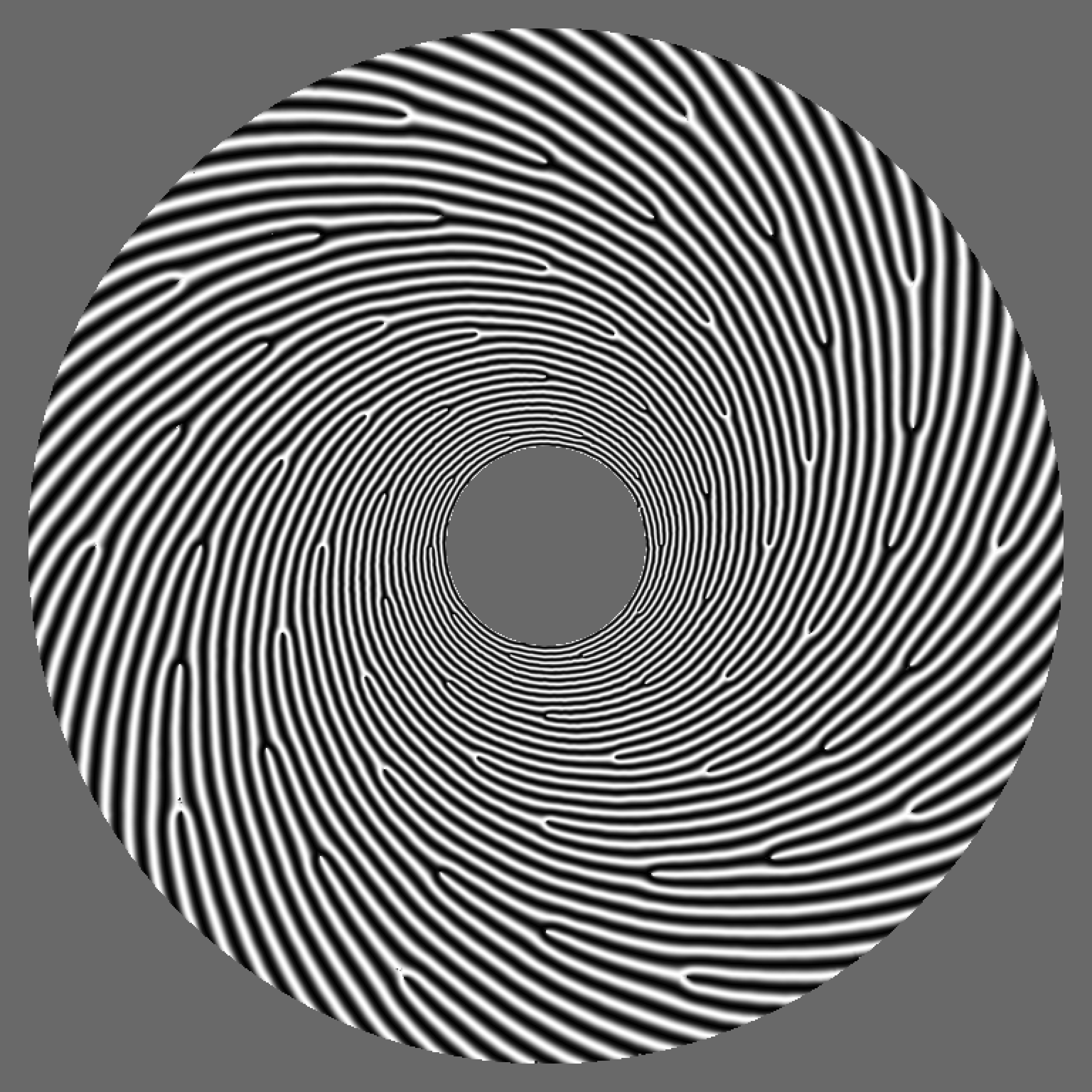
Figure 6: Reconstructed image from the LS tensor driven phase of noisy Fig. 2.

We show in Fig. 6, the image reconstructed from the LS tensor driven phase of the noisy original (given in Fig. 2) via the same technique. As can be verified visually, i) it is not identical to the original which contains noise, ii) the method has instead reconstructed nearly unflawed not only ridge waves (as can be expected because these are linearly symmetric), but also minutiae perfectly, despite SPR noise, and iii) The mapping $\Re\exp(i\Phi^{LS})$ is invariant to $\pm\bm{\omega}$ and $j2\pi$ translations of the phase, explaining the “disappearance” of the artifacts. In summary,

$$\{\bm{S}^{D},\bm{S}^{S},\Re\exp(i\Phi^{LS})\}$$ (16)

is a continuous and isotropic representation of phase where $\Re\exp(i\Phi^{LS})$ applies directional smoothing respecting phase discontinuities.

These and similar tests provide evidence for that, i) Linear Symmetry Tensors $\bm{S}^{D}$ and $\bm{S}^{S}$ are able to estimate $\bm{\omega}$ (save the sign), and ii) artifacts obey the theory in Section 3.1,3.2 and can be accounted for by appropriate mapping of $\Phi^{LS}$, e.g. (15) iii) LS tensor driven phase is sufficient for reconstructing the (amplitude normalized) original with unnoticable errors by human and computer vision, including in regions having either artifact discontinuity.

6 Gradient of LS tensor driven phase

6.1 Direct Gradient

Real and imaginary parts of Gabor filter responses,

$$z_{\bm{\omega}(f)}=u+iv=\exp(i\Phi^{LS})$$ (17)

are differentiable, where the amplitude $|z_{\bm{\omega}(f)}|$ is set to 1, without loss of generality. The dependence of $f,u,v,\Phi^{LS}$, and $z_{\bm{\omega}(f)}$ on $\bm{r}$ is not spelled out to reduce clutter. Consequently, the Gradient is given by

$$\nabla\Phi^{LS}=-v\nabla u+u\nabla v$$ (18)

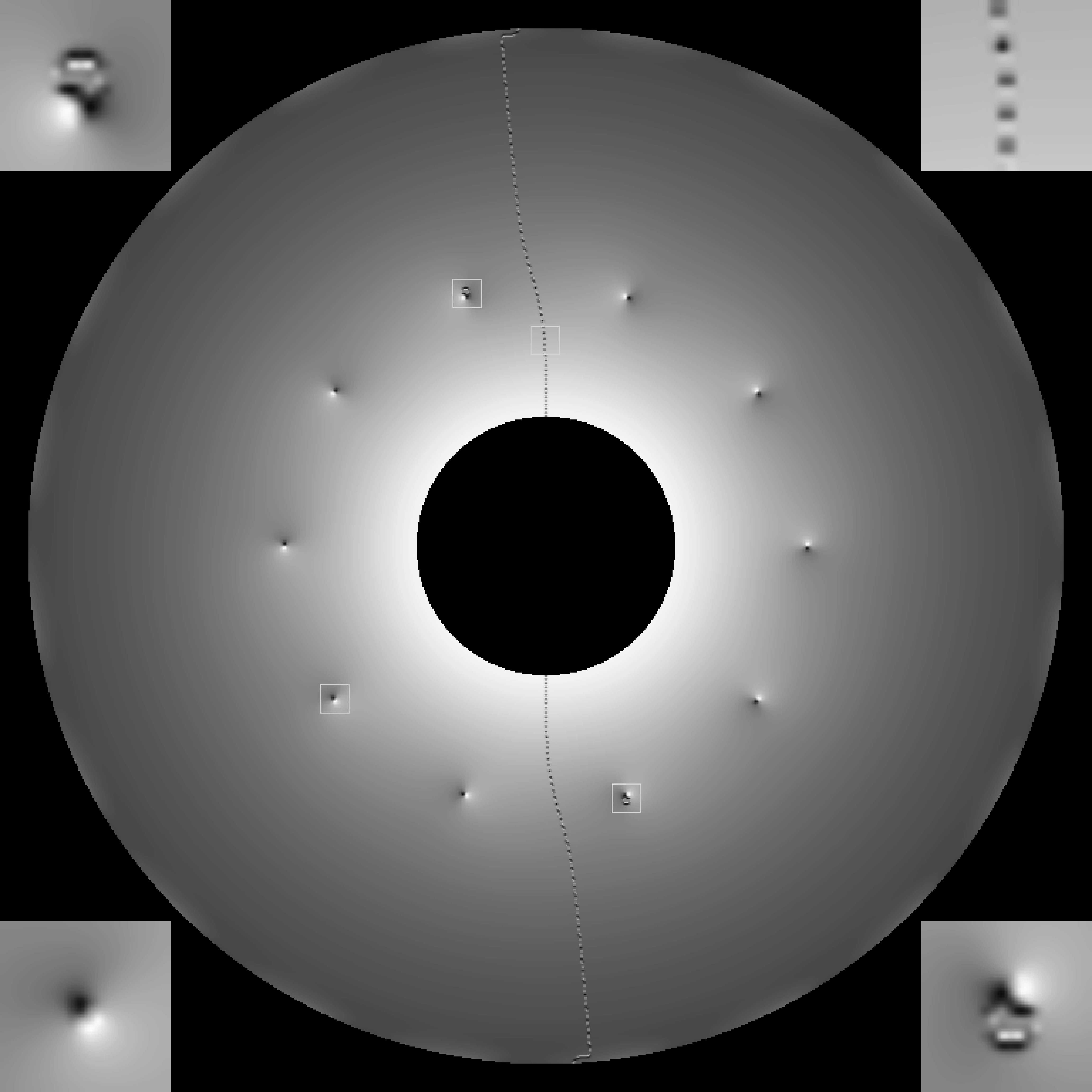
Figure 7: Magnitude of LS tensor driven phase gradient, $\|\nabla\Phi^{LS}\|$, direct implementation. Input is Fig. 1 (TR). Zoomed squares are inset at closest corners.

Fig. 7 shows the magnitude of gradients $\|\nabla\Phi^{LS}\|$ according to (18), evidencing that it is continuous at circular artifacts but not at all at hyper-plane ones despite that the input and its phase (Fig 1 TR and DL) are essentially noise-free. Circular artifacts in phase do not cause artifacts in gradients because phase gap at a presumed circular discontinuity point $\bm{r}$ is $2\pi$ which is in turn equivalent to multiplying $z_{\bm{\omega}(f)}$ with $\exp(i2\pi)=1$, causing no difference in $u,v$, nor in $\nabla u,$ and $\nabla v$ of (18).

In non-minutia neighborhoods of mid vertical portion, (zoomed in at T-R), local images are planar waves with constant $\bm{\omega}$, (8), obeying $\bm{\omega}^{T}\bm{\hat{n}}=0$. Here hyper-plane artifacts clearly survive standard implementation of derivation operator defying the intuition inherited from $\mathop{1\mathchar 45\relax D}$. The phase difference in neighboring pixels is no longer an integer multiple of $2\pi$ but can be as much as $2|\bm{\omega}^{T}\bm{r}|$. This is noticable in gradient magnitudes, as a zig-zag patterned artifact wave.

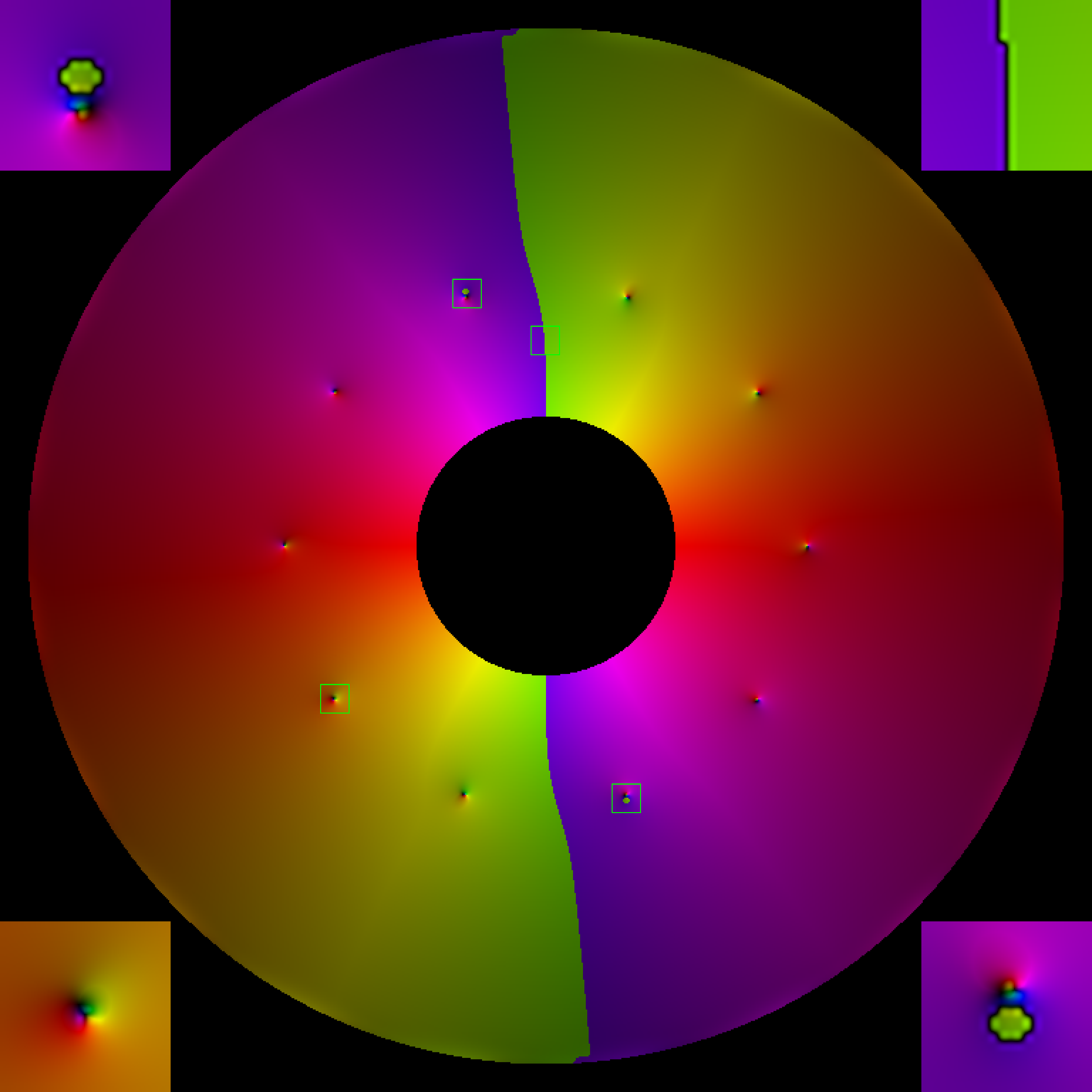
Figure 8: LS tensor driven phase gradient, $\nabla\Phi^{LS}$, compound implementation. Zoomed squares are inset at closest corners.

Unsurprisingly, hyper-plane artifacts plague even other neighborhoods with minutiae having directions aligned with $\bm{\hat{n}}$ or close to it. Therein one can observe that artifacts compared to other minutiae neighborhoods are prominent, Figure 8 zoomed in. Using the simple, one-minutia model in (8), which also has the minutia at the origin, the gradient field around such a minutia yields

$$\tilde{\nabla}\Phi^{LS}=\tilde{\bm{\omega}}+\frac{1}{r}\exp(i(\varphi+\pi/2))$$ (19)

in complex representation (since $\arg(\frac{\tilde{\bm{r}}}{i\tilde{\bm{\omega}}})=(\varphi-\pi/2-\arg(\tilde{\bm{\omega}})$). That is, the term $\tilde{\bm{\omega}}$ will dominate the gradient at sufficiently large distances $r$ from the origin(=minutia), i.e. at $1/\omega<r$. However, $\tilde{\bm{\omega}}$ is peculiar because if it is on the hyper-plane it will cause discontinuities. That is why hyper-plane artifacts will affect even gradients of horizontal minutiae (due to $\bm{\omega}^{T}\bm{\hat{n}}=0$ therein).

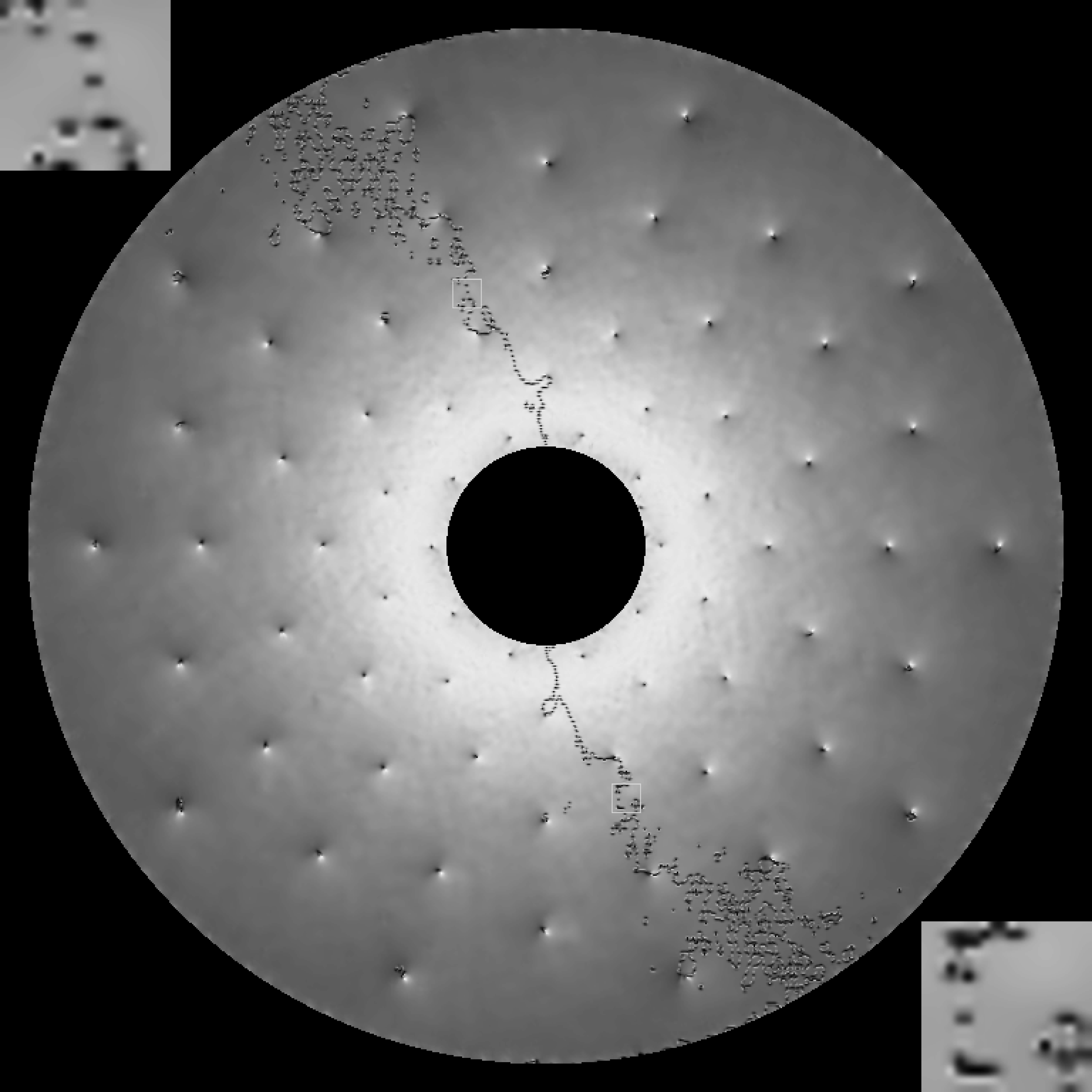
Figure 9: Magnitude of LS tensor driven phasegradient, $\|\nabla\Phi^{LS}\|$, direct implementation. Zoomed squares are inset at closest corners. Input image is the noisy Fig. 2.

Similarly, Fig. 9 is the direct implementation of Gradient magnitudes, via (18), for the input of Fig. 2, having minutiae at a wider range of scales. One observes the same type of artifacts, i.e. near minutiae having horizontal directions and at ridges with horizontal wave-fronts.

The overriding explanation is that the phase gradient will fluctuate $\pm\bm{\omega}$ at points having gradient directions in the hyper-plane. Phase gaps between neighboring points can then be as much as $2|\bm{\omega}^{T}\bm{r}|$, which also depends on $\bm{r}$. Standard gradient implementations will then have random jumps in vicinity of such points, expressed as a zig-zag artifact.

Consequently, to avoid hyper-plane artifacts in $\|\nabla\Phi^{LS}\|$, where phase gradient magnitude is $\|\bm{\omega}\|$ and should be continuous even if $\bm{\omega}$ is multiplied with $\pm 1$ at random, one must implement gradient operation differently. This is suggested here next, where the method exploits the direction of $\bm{\omega}$ such that the risk of producing vanishing $\bm{\omega}^{T}\bm{\hat{n}}=0$ is eliminated by using multiple $\bm{\hat{n}}$s. Direct implementation of gradient5 via (18) lacks the needed provision.

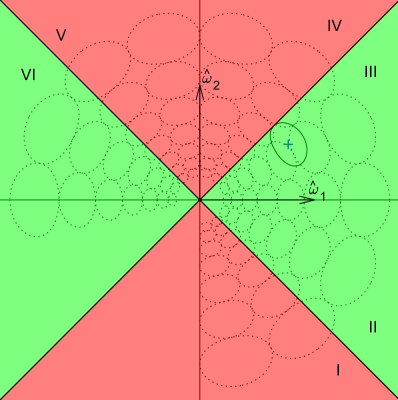
Figure 10: FT in $\mathop{2\mathchar 45\relax D}$ with two different analytic signal representations of the same signal, 1-IV being the first with $\bm{\hat{n}}=\hat{\bm{\omega}}_{1}$ and III-VI being the second with $\bm{\hat{n}}=\hat{\bm{\omega}}_{2}$. Green II-III marks the region that is safest with $\bm{\hat{n}}=\hat{\bm{\omega}}_{1}$. Iso curves of Gabor filters for inputs with different $\bm{\omega}$ are in black.

6.2 Compound gradients and their magnitudes

We detail compound implementation in $\mathop{2\mathchar 45\relax D}$, Fig. 10, for pedagogical reasons. The idea will be extended to $\mathop{N\mathchar 45\relax D}$ subsequently. Let $\hat{\bm{\omega}}_{1}$, $\hat{\bm{\omega}}_{2}$, be basis vectors of 2D FT domain. We assume that the walking direction vector is, $\bm{\hat{n}}=\hat{\bm{\omega}}_{1}$. Then the specific input sinusoid, $f(\bm{r})=\cos(\omega\hat{\bm{\omega}}_{1}^{T}\bm{r})$, with $\bm{\omega}$ located in $\pm\pi/4$ around $\bm{\omega}_{1}$ will produce the most reliable phase. By contrast, if the walking direction $\bm{\hat{n}}=\hat{\bm{\omega}}_{2}$ would have been assumed, the $\bm{\omega}$ of the input sinusoid in region $\pm\pi/4$ around $\bm{\omega}_{2}$ would produce the most reliable phase.

By using two different representations, $\bm{\hat{n}}\!=\!\hat{\bm{\omega}}_{1}$, and $\bm{\hat{n}}\!=\!\hat{\bm{\omega}}_{2}$ respectively, one can obtain two phases $\Phi_{1}^{LS}$ and $\Phi_{2}^{LS}$ having different reliabilities. Each signal representation would then have its own half-space of FT where the FT of the respective analytic function $z_{\bm{\omega}(f)}$ is non-zero (and zero). This requires the additional knowledge of $\Phi^{LS}_{2}$, which can be construed from $\Phi^{LS}_{1}$,

$$\Phi^{LS}_{2}(\bm{r})=\operatorname{sgn}(\hat{\bm{\omega}}_{2}^{T}\bm{\omega}(\bm{r}))\Phi^{LS}_{1}(\bm{r})$$ (20)

One can then expect that $\|\nabla\Phi_{1}^{LS}\|=\|\nabla\Phi_{2}^{LS}\|=\omega$ will be continuous when $\bm{\omega}$ is at a comfortable distance from the applicable hyper-plane.

After defining the index $J$

$$J(\bm{r})=\operatorname*{argmax}_{j}\{|\hat{\bm{\omega}}_{j}^{T}\bm{\omega}(\bm{r})|\}_{j=1}^{N=2}$$ (21)

identifying the most reliable phase, we can apply gradient to $\Phi^{LS}_{1}$, and $\Phi^{LS}_{2}$, yielding the compound gradient

$$\nabla\Phi^{LS}(\bm{r})=\operatorname{sgn}(\hat{\bm{\omega}}_{J}^{T}\bm{\omega}(\bm{r}))\nabla\Phi^{LS}_{J}(\bm{r})$$ (22)

where $\operatorname{sgn}$ is the sign function. To reduce symbol clutter, we represent compound gradients in the same way as gradients by $\nabla$. The gradient direction has thereby sign-rectification to assure that $\bm{\omega}$ (computed by LS tensor) points into the reference non-zero zone. We recall that there are two Gabor decompositions involved, but only one of them serves as the reference defining the half plane in which aggregated “$\bm{\omega}$”s are delivered.

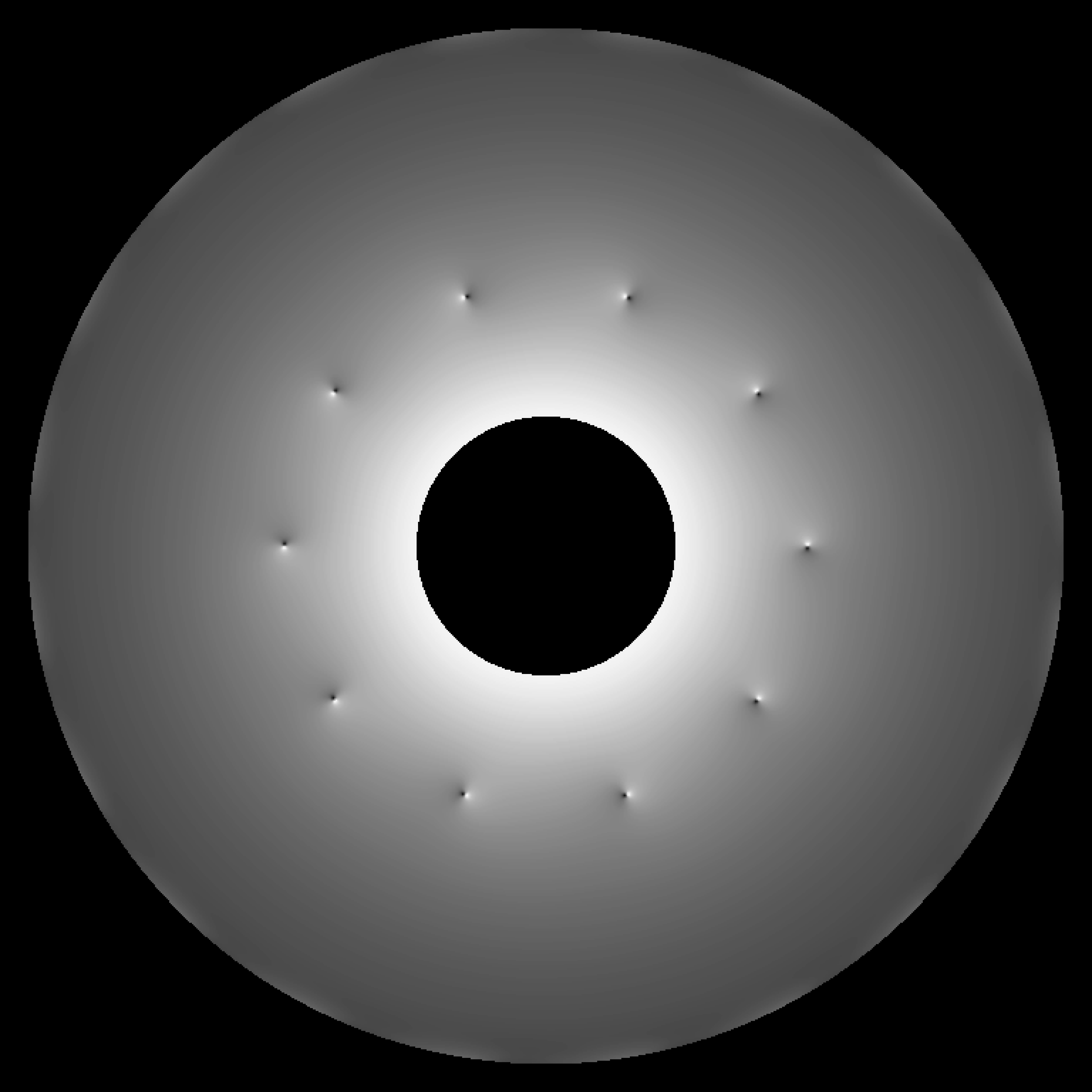
Figure 11: Magnitude of LS tensor driven phase gradient, $\|\nabla\Phi^{LS}\|$, compound implementation. The input is Fig. 1 (R;T).

Fig. 11 shows the magnitude of the compound gradient, $\|\nabla\Phi^{LS}\|^{2}$, computed via (22). It depicts no zig-zag patterned artifacts, the hallmark of hyper-plane discontinuity. Fig. 8 shows gradient vectors in color (HSV), showing that magnitude wise discontinuity has been eliminated.

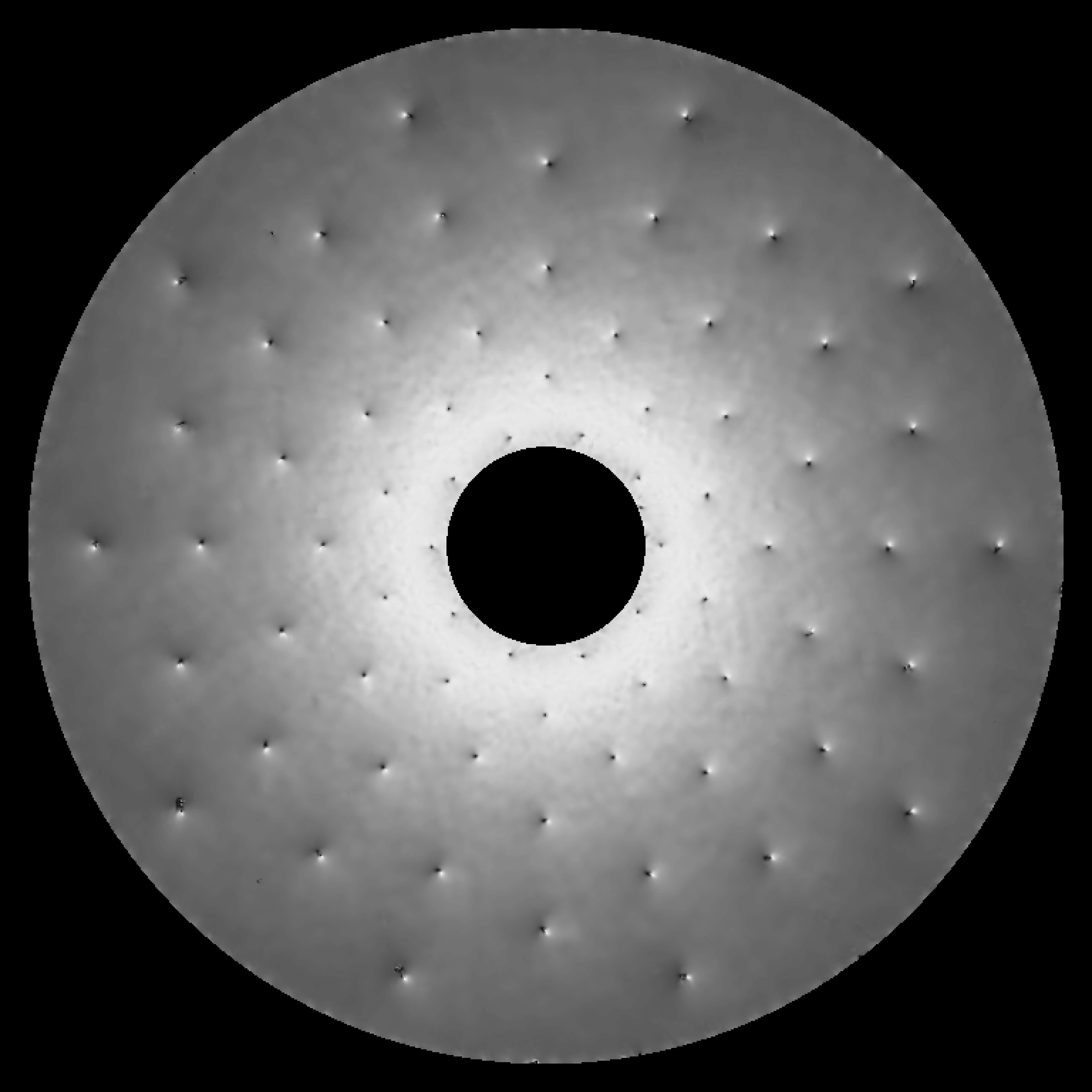
Figure 12: Magnitude of LS tensor driven phasegradient, $\|\nabla\Phi^{LS}\|$, compound implementation. Input image is the noisy Fig. 2.

Likewise, Fig. 12, which is computed for the noisy multi minutia image 2, the brightness is continuous. The brightness is modulated by the magnitude $\|\nabla\Phi^{LS}\|$, where the gradient is obtained by compound gradient method above.

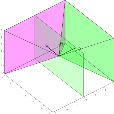
Figure 13: FT in $\mathop{3\mathchar 45\relax D}$ with its reliable pyramid (green) under the assumption $\bm{\hat{n}}=\hat{\bm{\omega}}_{1}$ defining the (green) hyper-plane. Ditto pyramid (pink), but for the alternative $\bm{\hat{n}}=\hat{\bm{\omega}}_{2}$ (hyper-plane not drawn).

Compound gradient implementation and conclusions above can be generalized to $\mathop{N\mathchar 45\relax D}$ in a straight forward manner. Assuming an analytic signal having $\bm{\hat{n}}=\hat{\bm{\omega}}_{1}$, the region of most reliable phase in the FT space is a hyper-pyramid around $\bm{\hat{n}}$, green ”Egyptian pyramid” in Fig. 13. The least reliable region is the remainder of the non-zero zone, i.e. $N-1$ half hyper-pyramids between the reliable hyper-pyramid and the hyper-plane $\bm{\hat{n}}^{T}\bm{\omega}=0$, marked green in the figure. Phase being $\Phi^{LS}_{1}$ under the presumption (of $\bm{\hat{n}}=\hat{\bm{\omega}}_{1}$), $N-1$ alternative phases $\Phi^{LS}_{2},\cdots\Phi^{LS}_{N}$ can be construed from it based on respective presumptions on walking directions, $\bm{\hat{n}}=\hat{\bm{\omega}}_{2},\cdots\bm{\hat{n}}=\hat{\bm{\omega}}_{3}$ (without filtering with Gabor filters anew) via:

$$\Phi^{LS}_{j}(\bm{r})=\operatorname{sgn}(\hat{\bm{\omega}}_{j}^{T}\bm{\omega}(\bm{r}))\Phi^{LS}_{1}(\bm{r})\quad j\in 2\cdots N$$ (23)

Each $\Phi^{LS}_{j}$ has its own reliable hyper-pyramid. Such a pyramid is marked as pink in $\mathop{3\mathchar 45\relax D}$ in the figure for $\Phi^{LS}_{2}$.

A compound phase gradient is then sewn together by cherry-picking among phase gradients of reliable pyramids. A practical way of achieving this is by using the index $J$

$$J(\bm{r})=\operatorname*{argmax}_{j}(\{|\hat{\bm{\omega}}_{j}^{T}\bm{\omega}(\bm{r})|\}_{j})\qquad j,J\in 1\cdots N$$ (24)

It identifies the most reliable hyper-pyramid in which $\bm{\omega}(\bm{r})$ is. The ambiguity when max is not unique (at hyper-pyramid boundaries), is resolved e.g. by setting J as min of (two) $j$s in the cause. Note that $\bm{\omega}(\bm{r})$ is always located in the non-zero zone of the FT partition produced by the $\bm{\hat{n}}=\hat{\bm{\omega}}_{1}$ assumption, albeit the location can be in its non-reliable zone. In the latter case, the location can be in the zero zone of another partitioning of the FT space.

A phase gradient selection, the analog of (22), decided by $J$ produces finally the compound gradient.

$$\nabla\Phi^{LS}(\bm{r})\!=\!\operatorname{sgn}(\hat{\bm{\omega}}_{J(\bm{r})}^{T}\bm{\omega}(\bm{r}))\nabla\Phi^{LS}_{J(\bm{r})}(\bm{r})$$ (25)

Apart from book-keeping cost of constructing $\operatorname{sgn}(\bm{\omega}_{j}^{T}\bm{\omega}(\bm{r}))$, and $J(\bm{r})$, compound gradients can be obtained at the same cost as direct implementation. This is because $J(\bm{r})$ can be used to compute not more than one $\nabla\Phi^{LS}_{J(\bm{r})}(\bm{r})$ per point $\bm{r}$. Book-keeping cost is at the order of $N^{2}$ arithmetic operations per point, if projections $\bm{\omega}_{j}^{T}\bm{\omega}$ are computed directly. However, rather than projections, look-up tables on components of $\bm{\omega}$ can be used to decide signs and orderings of $\bm{\omega}_{j}^{T}\bm{\omega}$, marginalizing the overhead.

In summary, the compound phase gradient

$$\{\bm{S}^{D},\bm{S}^{S},\Re\exp(i\Phi^{LS}),\|\nabla\Phi^{LS}\|\}$$ (26)

is a continuous and isotropic representation in magnitude.

6.3 LS tensor of Phase

The direction of phase gradient remains discontinuous across neighborhoods with wave vectors in the Analytic Signal hyper-plane. This means that while $\|\nabla\Phi^{LS}\|$ is continuous for use in applications (e.g. it can be smoothed) when implemented via compound gradient, $\nabla\Phi^{LS}$ is not continuous. Compound gradient achieves continuity of norms of gradients but falls short of providing the same for their directions.

We suggest the LS tensor of phase, as an alternative to gradient of phase and a remedy to its directional discontinuity, in applications. This is defined as the (infinitesimal) Linear Symmetry Tensor of Phase here next. The phase is then implemented as LS tensor driven phase, whereas the gradient is implemented as compound gradient.

$$\|\bm{\omega}\|^{-\gamma}\nabla\Phi^{LS}\nabla^{T}\!\Phi^{LS}$$ (27)

The choice and effect of $\gamma$ is discussed further below. For now we set $\gamma=0$ to ease the discussion.

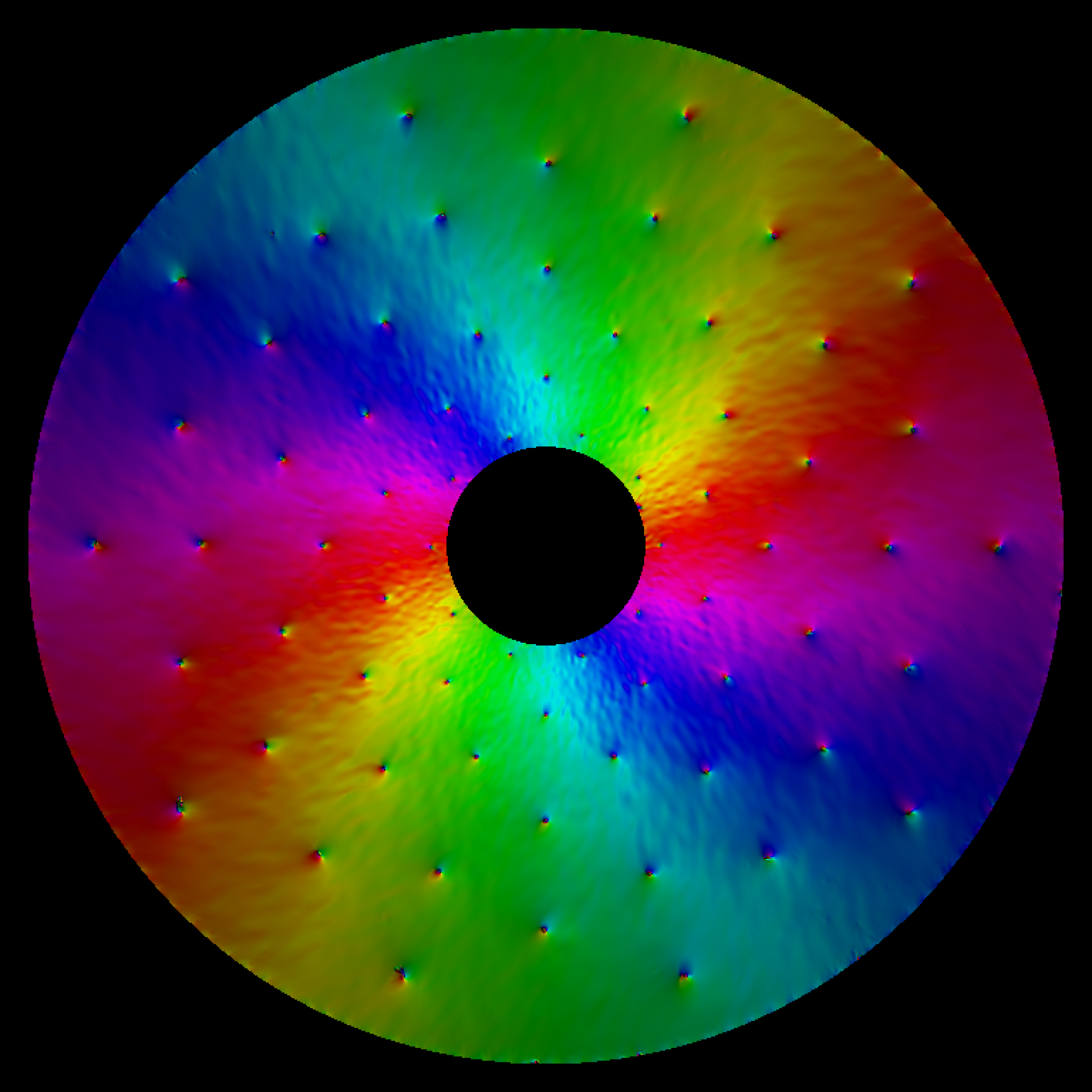
Figure 14: Complex image with pixels representing $(\tilde{\nabla}\Phi^{LS})^{2}$ eliminating hyper-plane artifacts. Hue and intensity depict angles and magnitudes of complex pixels. Input image is the noisy Fig. 2.

In 2D, LS tensor is equivalent to complex squaring of the gradient [5], when the gradient is represented as a complex number i.e. $(\tilde{\nabla}\Phi^{LS})^{2}$. The tensor is illustrated in Fig. 14, with hue depicting the direction of “squared gradients”. That neither magnitude nor direction suffer from hyper-plane artifacts is evidenced by the image. Additionally, this tensor can be averaged (as opposed to $\nabla\Phi^{LS}$ vectors), suggesting better estimates of the local direction and the scale, $2\pi/\|\bm{\omega}\|$ [6],[28]. An application of this representation of phase gradients showing its usefulness is readily presented in the next section.

In applications, when averaging $\nabla\Phi^{LS}\nabla^{T}\Phi^{LS}$, the highest absolute frequencies will dominate the average due to the inherent squaring and cross products in the tensor. To give absolute frequencies uniform weight, when used in subsequent operations, e.g. averaging, one could use $\|\bm{\omega}\|^{-1}\nabla\Phi^{LS}\nabla^{T}\Phi^{LS}$ which corresponds to $\gamma=1$ in (27). Generally, to have steerable weights of scales comprised in local images can be desirable in applications, e.g. higher weights to low absolute frequencies, which can be achieved by using different values of $\gamma$. This adaptation is also known as gamma correction from computer display technologies which try to render color synthesis to match human expectations.

In summary,

$$\{\bm{S}^{D},\bm{S}^{S},\Re\exp(i\Phi^{LS}),\|\bm{\omega}\|^{-\gamma}\nabla\Phi^{LS}\nabla^{T}\!\Phi^{LS}\}$$ (28)

is a continuous and isotropic representation of phase gradients which can be smoothed.

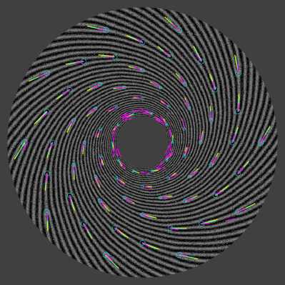
Figure 15: Detected minutiae aggregated over multiple scales overlaid the original, as suggested here (yellow). Detected minutiae by baseline method mindtct [34] (pink). Ground truth periods and locations are indicated as circles and dashed lines (cyan).

7 Minutia scale space and LS of phase in $\mathop{2\mathchar 45\relax D}$

Applying LS tensor to the phase of the single minutia fingerprint minutia model, (8), where $r,\varphi$ are local coordinates, yields

$$(\tilde{\nabla}\Phi^{LS})^{2}=\tilde{\bm{\omega}}^{2}+\frac{2i\tilde{\bm{\omega}}}{r}\exp(i\varphi)-\frac{1}{r^{2}}\exp(i2\varphi)$$ (29)

Projecting this on a filter with phase term $w=i\exp(i\varphi)$ will annihilate the first and the third component (because $\exp(i\varphi)$ is orthogonal to $\exp(i2\varphi)$), resulting in a (high magnitude) complex value sharing direction with $\tilde{\bm{\omega}}$ at the minutia location. A pixel magnitude will indicate the certainty of the location to be a minutia, and the argument the minutia direction (ISO standard). Additionally, minutia period, $T=2\pi/\|\bm{\omega}\|$ via $\|\bm{\omega}\|=\|\nabla\Phi^{LS}\|$ will be obtained, which is a novelty. These are evidenced in Fig. ​15, which (in yellow) shows the found minutiae from magnitude thresholded complex image added to a dimmed version of the original for convenience. Magnitudes depict automatically estimated minutia periods.

One could also project neighborhoods of $(\tilde{\nabla}\Phi^{LS})^{2}$ on $w^{2}$, (29). This will annihilate the first and the second terms, retaining the third term of the equation, which will yield an additional manner to obtain the minutia location. Although, the direction information $\tilde{\bm{\omega}}$ vanishes, the result can nonetheless be useful, e.g. as a second piece of evidence for minutia location in noisy images, complementing the projection on $w$. Such projections define a formalism for minutia location, direction and type determination via complex convolutions as LS tensor of phase is continuous, both in direction and magnitude. .

It is desirable to extract minutia scale accurately, too. This is because, the filter $w$ has a fixed size and convolution (even when complex) is linear yielding in that minutiae can be detected only within a certain range of scales. This is due to the fact that FT of linear filters must attenuate as the absolute frequency increases. However, large variations of scale can occur within the same fingerprint, in addition to between different fingerprints for natural reasons. Next we suggest a formalism addressing multi-scale minutia modeling and detection, within LS tensor driven phase computations.

As scale, we have suggested to use $T=2\pi/\|\bm{\omega}\|$ where $\|\bm{\omega}\|$ is the absolute frequency employed in LS tensor driven phase. Though not exactly the same, this is an analogue of the scale concept of [37], [13],[28] with main differences being that our scale is based on a non-linear scale space produced by the $\bm{S}^{S}$, our scale tensor based on the trace of $\bm{S}^{D}$, which is the Linear Symmetry Tensor of the input but using multiple “$\sigma$”s in derivations. In the method, the logarithm of trace is used at fixed samples of $\sigma$ to interpolate the $\bm{\omega}$ when driving our Gabor filter selection process. Thereby $\|\bm{\omega}\|$ is already estimated when LS tensor driven phase is so that additional scale estimations for fingerprint period calculations are not necessary.

To locate, and compute minutia direction, scale and type is done in three steps where the input is the LS tensor of phase, as shown in Fig. 14 for the multi-scale, noisy minutiae image, Fig. 2.

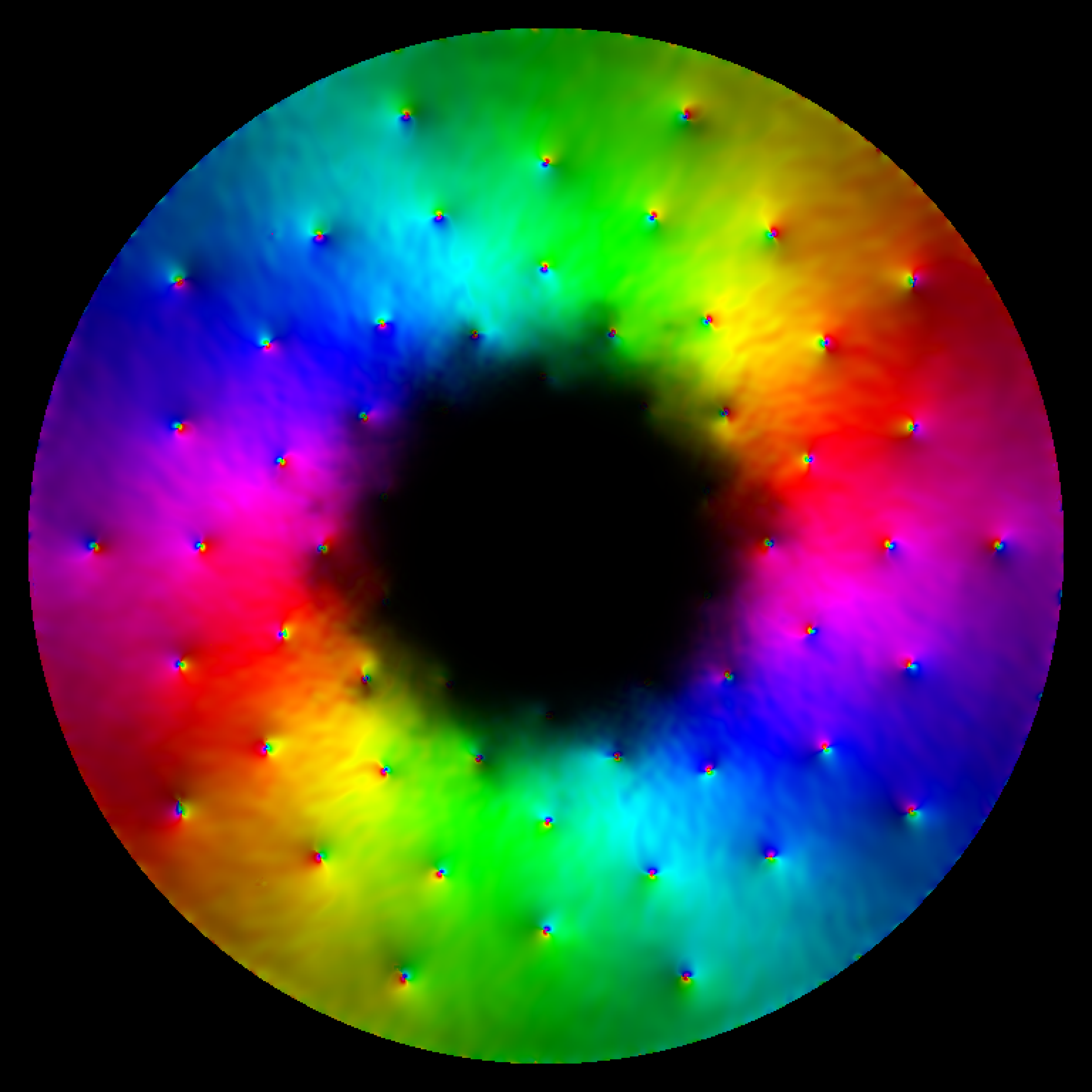
Figure 16: One scale of $(\tilde{\nabla}\Phi^{LS})^{2}$ corresponding to Fig. 2 which is convolved with scale adapted complex filter $w$ to find minutiae.

1. The available range of $\|\bm{\omega}\|$ in the LS tensor of phase, Fig. 14, is partitioned into overlapping intervals. The purpose is to use multiple complex detection filters $w$ since minutiae have scale variations even in the same fingerprint. Here, we have deliberately used three (instead of e.g. seven) partitions to illustrate the point, that it is permissible not to know the actual “number” of scales a priori. Thus, using such arbitrary partitions, we have replaced $|\tilde{\nabla}\Phi^{LS}|^{2}$ with belongingness value, $\beta(\|\bm{\omega}\|)=\exp(-|\|\bm{\omega}\|-\|\bm{\omega}_{p}\||^{2}/(2\sigma_{p}^{2}))$ where $\|\bm{\omega}_{p}\|$ are partition centers. The result is the belongingness, [38], of the estimated $\|\bm{\omega}\|$ at an image location to the scale partition. The variance $\sigma_{p}^{2}$ is chosen such that the distance to the next partition center is $\approx 3\sigma_{p}$, where $\beta$ reduces to insignificance. Fig. 16 shows one of the three scales, $p$, in HSV colors. Pixel magnitudes represent now belongingness to the scale interval denoted with the index $p$, (not $|\tilde{\nabla}\Phi^{LS}|^{2}$) whereas pixel arguments are unchanged (i.e. double angles of compound gradients $\angle(\tilde{\nabla}\Phi^{LS})^{2}$).

   

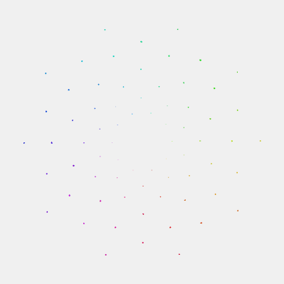
   Figure 17: Minutia detection by complex filtering where hue represents direction angles of minutiae, in HSV color standard using noisy Fig. 2 as input. However, we have given zero pixels white value (instead of black) in the image to improve the visibility of colored points, representing minutiae. All 70 minutiae comprising 7 different scales are detected with correct angles, see also Fig. 15.

2. To each such complex map, one complex filter $w_{p}$ with size according with the partition center, was applied to detect minutiae via convolution. Detection results from all belongingness maps were subsequently aggregated by choosing the maximum magnitude responses, yielding a single minutia map. In the aggregated result, complex pixels are expected to have large magnitudes and correct minutia angles at minutia locations, and small magnitudes (near zero) in non-minutia locations which is the case, see Fig. 17.

3. Magnitudes of (complex) pixels are blob like and large at minutia locations in the resulting image. These can be refined by a centroid finding algorithm to obtain one minutiae location per blob. The corresponding minutia directions can be retained from arguments of complex pixel results of the previous step, at centroids. Scales of minutia can be retained from the exact $T$s retained from the original LS tensor of phase map in the first step, before creating belongingness partitions. The result is illustrated in Fig. 15.

8 Experiments

Table 1 compares the detection accuracies of our and a baseline method, mindtct [34], when we have increased the noise amount until the present method started to deteriorate from 0 % FR, FA error level. This happened when SNR was 0.61, e.g., Fig. 2, when Salt & Pepper replacement, SPR, noise, is used as a contaminator. The baseline was then operating at 34% FA, and 20% FR error (pink, in Fig. 15) versus ours 0% and 0% respectively. Detection is deemed correct if minutia location is within half the minutia period, which is known for every minutia, from the ground truth location. The color cyan represents ground truths, which include locations, directions and periods. Periods are shown in two ways for convenience of comparison: as circles and as vector magnitudes.

Table 2 shows statistics of correctly detected minutiae. Our estimation of period was having a mean (relative) error of 0.09 with remarkably low standard deviation, 0.03, suggesting a stable estimation of periods. Investigating period estimations closer, we found to our surprise that ground truth periods, $T_{j}$, were systematically less than estimated periods $T$. The average bias, i.e. the average of $\Delta T/T_{j}$ (without absolute value) was 0.07. This is however reasonable and explained by that the (replacement) noise increases the observed frequency of input patches, hence the period was observed as reduced. Period estimation was not available with mindtct method.

Direction estimation errors were within 0.07 radians for our method, and 0.14 radians for the baseline. The standard deviation of direction estimations, was significantly lower in the present method, 0.06, than mindtct 0.39 indicating more accuracy and stability of direction.

Means of localization errors for detected minutiae (by respective method) were slightly in favor of mindtct than our method, 0.15 versus 0.25, with essentially the same standard deviation, 0.08 versus 0.09. On the other hand, our result includes minutiae that were missed by mindtct all together which are not in the statistics of mindtct performance.

Detection instability reaches minutiae with larger periods with increased noise, although graceful degradation is less systematic for mindtct, e.g., the false (pink) minutia near BR corner, Fig. 15. The observation confirms that fingerprints of young children are more vulnerable to noise than adults at the currently practiced imaging resolution (510 dpi i.e., the mid-scale in Fig. 2, 15) and in commonly used algorithms.

Present Mindtct

FR FA 0.0 0.0 0.20 0.34

Table 1: Performance of minutia detection in degraded images).

	${|\Delta\bm{r}|/T_{j}}$	${|\Delta\theta|}$	${|\Delta T|/T_{j}}$
Present
$\mu$	0.25	0.07	0.09
$\sigma$	0.09	0.06	0.03
Mindtct
$\mu$	0.15	0.14	N/A
$\sigma$	0.08	0.39	N/A

Table 2: Error statistics of locations, directions and periods of detected minutiae in degraded images. Means and standard deviations are in rows marked with $\mu$ and $\sigma$. Location and period estimation errors are normalized with ground truth minutiae periods $T_{j}$ so that all errors are dimensionless.

9 Conclusions

Our main conclusions are listed as follows.

• Representation of phase via

  $$\{\bm{S}^{D},\bm{S}^{S},\Re\exp(i\Phi^{LS})\}$$ (30)

  is continuous and isotropic. The representation is useful in image denoising.

• Vector representation of phase gradient

  $$\{\bm{S}^{D},\bm{S}^{S},\Re\exp(i\Phi^{LS}),\|\nabla\Phi^{LS}\|\}$$ (31)

  is continuous and isotropic in magnitude, if compound gradients are used.

• LS tensor of phase

  $$\{\bm{S}^{D},\bm{S}^{S},\Re\exp(i\Phi^{LS}),\|\bm{\omega}\|^{-\gamma}\nabla\Phi^{LS}\nabla^{T}\Phi^{LS}\}$$ (32)

  is continuous and isotropic in magnitude and orientation, if compound gradients are used. This can be attractive to applications as an alternative to phase gradient vectors lacking directional continuity.

• Synthetic images can be produced upon the user sets type, direction, period of minutia, the number of minutiae per scale, and the number of scales. In the resul i) minutiae are embedded in all ridge directions in a dense range of ridge periods $(T_{\min},T_{\max})$; ii) ground truths w.r.t. directions and periods at any accuracy are available at all image locations; iii) no new minutiae are created other than those specified.

• LS tensors of phase can be used to detect physical (non-artifact) discontinuities, e.g. minutiae. Robust detection via multi-scales is possible since scale is inherently estimated in the LS tensor of phase, (27).

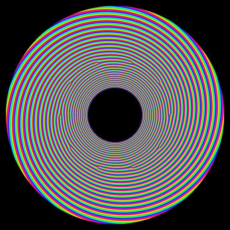
Figure 18: (Continuous phase as in Fig. 1 (Top-L) but represented in HSV colors, with Saturation set to max;

Appendix

Fig. 18 is the same image as the synthesized phase image shown in Fig. 1 T,L but represented in HSV colors, with Hue modulated by the phase. Value and Saturation are set to max. As Hue is an angle in this representation, there are no discontinuities except those at minutiae.

Fig. 1 T,R is shown in Fig. 19 where Hue modulates the LS tensor driven phase. Radially, colors are not displaying discontinuities anymore (in comparison to Fig. 1 T,R) and colors are the same as those in Fig. 18 except in the left half. This leads to the discontinuity observed in the mid-vertical portion. Phase the left half differs from the ground-truth with $\pi$ since Analytic Signal knows about only $\bm{\omega}$ residing in one half of FT domain, since Gabor filters exist only there.

Continuity in the radial direction is explained by that angles are rendered by Hue and are equivalent up to $2\pi k$ addition in HSV color scheme, causing no perceivable jumps. This shows that i) phase jumps at circular discontinuities equal to $2\pi$ (else they would be visible since they were present in all directions, see Fig. 1 T,R.) ii) whether this is a problem depends on how phase is represented and if the continuous phase is actually needed. If needed, a phase reconstruction algorithm must be applied to Gabor phase, as a color representation will not suffice.

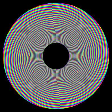
Figure 19: LS tensor driven phase in HSV colors corresponding to Fig. 1 (Down-L).

By contrast, hyper-plane discontinuities are noticable discontinuities even in HSV representation recognized by that i) gaps do not equal to $2\pi$ at discontinuities except very rarely, and ii) discontinuities occur always at boundary of Gabor half space, i.e. waves with vectors $\bm{\hat{n}}^{T}\bm{r}=0$.

Fig. 20 shows in HSV color representation LS tensor driven phase of a fingerprint. In HSV representation, which is perception wise continuous in Hue (since Hue is an angle), is modulated by $\Phi^{LS}$ as estimated by LS tensor driven phase, (6). Thereby, circular discontinuities are suppressed by the mechanism rendering the color. Along horizontal ridges however, color discontinuities representing hyper-plane artifacts are visible. The image also evidences that synthetic images with known ground truths w.r.t. orientation, scale and phase simplify evaluation and identification of causes, consequences and effectiveness of remedies.

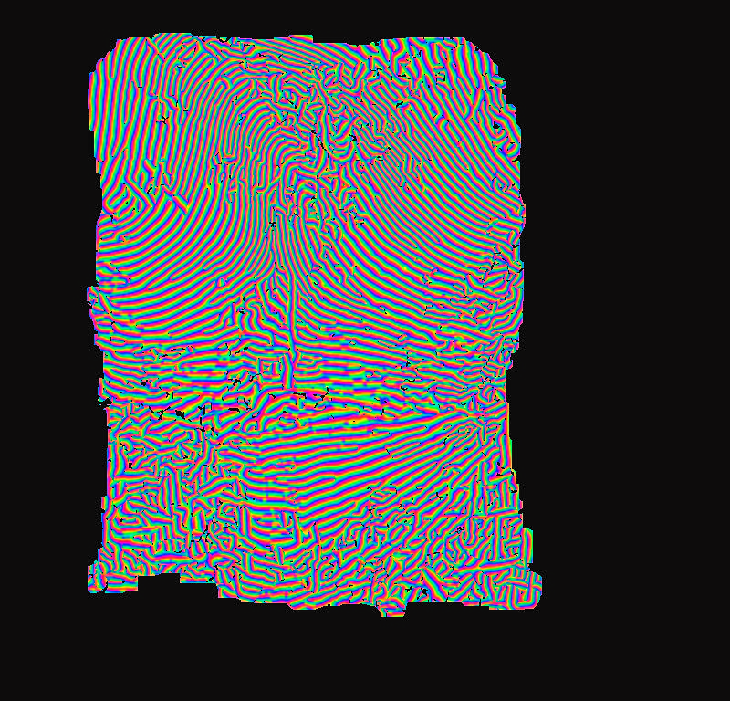
Figure 20: Fingerprint phase showing discontinuity near horizontal ridges

References

- [1] Martino Alessandrini, Olivier Bernard, Adrian Basarab, and Hervé Liebgott. Multiscale optical flow computation from the monogenic signal. IRBM, 34(1):33–37, 2013.
- [2] Basanta Bhaduri and Gabriel Popescu. Derivative method for phase retrieval in off-axis quantitative phase imaging. Optics letters, 37(11):1868–1870, 2012.
- [3] J. Bigun. Pattern recognition by detection of local symmetries. In E.S. Gelsema and L.N. Kanal, editors, Pattern recognition and artificial intelligence, pages 75–90. North-Holland, 1988.
- [4] J. Bigun. Vision with Direction. Springer, Heidelberg, 2006.
- [5] J. Bigun and G.H. Granlund. Optimal orientation detection of linear symmetry. In ICCV, London, June 8–11, pages 433–438. IEEE Computer Society, 1987.
- [6] Josef Bigun and Anna Mikaelyan. Frequency map by structure tensor in logarithmic scale space and forensic fingerprints. In Proceedings of the IEEE Conference on Computer Vision and Pattern Recognition Workshops, pages 136–145, 2016.
- [7] Kai Cao and Anil K Jain. Latent orientation field estimation via convolutional neural network. In Biometrics (ICB), 2015 International Conference on, pages 349–356. IEEE, 2015.
- [8] Raffaele Cappelli, Dario Maio, Alessandra Lumini, and Davide Maltoni. Fingerprint image reconstruction from standard templates. IEEE transactions on pattern analysis and machine intelligence, 29(9):1489–1503, 2007.
- [9] Mario Costantini. A novel phase unwrapping method based on network programming. IEEE Transactions on geoscience and remote sensing, 36(3):813–821, 1998.
- [10] Richard Delanghe and Fred Brackx. Hypercomplex function theory and hilbert modules with reproducing kernel. Proceedings of the London Mathematical Society, 3(3):545–576, 1978.
- [11] Michael Felsberg and Gerald Sommer. Structure multivector for local analysis of images. In Multi-image analysis, pages 93–104. Springer, 2001.
- [12] D.J. Fleet and A.D. Jepson. Computation of component image velocity from local phase information. International Journal of Computer Vision, 5(1):77–104, 1990.
- [13] LMJ Florack, BM ter Haar Romeny, JJ Koenderink, and MA Viergever. Linear scale-space. Journal of Mathematical Imaging and Vision, 4(4):325–351, 1994.
- [14] W. Förstner and E. Gülch. A fast operator for detection and precise location of distinct points, corners and centres of circular features. In Proc. Intercommission Conference on Fast Processing of Photogrammetric Data, Interlaken, pages 281–305, 1987.
- [15] M.D. Garris and R.M. McCabe. Nist special database 27: Fingerprint minutiae from latent and matching tenprint images. Technical report, NIST, Gaithersburg, MD, USA, 2000.
- [16] Dennis C Ghiglia and Mark D Pritt. Two-dimensional phase unwrapping: theory, algorithms, and software, volume 4. Wiley New York, 1998.
- [17] Enrico Glerean, Juha Salmi, Juha M Lahnakoski, Iiro P Jääskeläinen, and Mikko Sams. Functional magnetic resonance imaging phase synchronization as a measure of dynamic functional connectivity. Brain connectivity, 2(2):91–101, 2012.
- [18] Leif Haglund. Adaptive multidimensional filtering. PhD thesis, Linköping University Electronic Press, 1991.
- [19] C. Harris and M. Stephens. A combined corner and edge detector. In Proceedings of the fourth Alvey Vision Conference, pages 147–151, 1988.
- [20] B. Jähne. Spatio-Temporal Image Processing. LNCS 751. Springer, Heidelberg, 1993.
- [21] M. Kass and A. Witkin. Analyzing oriented patterns. Computer Vision, Graphics, and Image Processing, 37:362–385, 1987.
- [22] M. Kawagoe and A. Tojo. Fingerprint pattern classification. Pattern Recognition, 17:295–303, 1984.
- [23] H. Knutsson. Representing local structure using tensors. In Proceedings 6th Scandinavian Conf. on Image Analysis, Oulu, June, pages 244–251, 1989.
- [24] J.J. Koenderink and A.J. van Doorn. Receptive field families. Biol. Cybern., 63:291–298, 1990.
- [25] Peter Kovesi, Ben Richardson, Eun-Jung Holden, and Jeffrey Shragge. Phase-based image analysis of 3d seismic data. ASEG Extended Abstracts, 2012(1):1–4, 2012.
- [26] Kieran G Larkin. Natural demodulation of two-dimensional fringe patterns. ii. stationary phase analysis of the spiral phase quadrature transform. JOSA A, 18(8):1871–1881, 2001.
- [27] K. G. Larkin and P. A. Fletcher. A coherent framework for fingerprint analysis: are fingerprints holograms? Optics Express, 15(14):8667–8677, 2007.
- [28] T Lindeberg. Feature detection with automatic scale selection. International Journal of Computer Vision, 30(2):79–116, 1998.
- [29] G. Medioni, M.S. Lee, and C.K. Tang. A computational framework for segmentation and grouping. Elsevier, 2000.
- [30] A. Mikaelyan and J. Bigun. Ground truth and evaluation for latent fingerprint matching. In CVPR Workshop on Biometrics. IEEE-XPLORE, Piscataway, NJ, 6 2012.
- [31] Seiichi Nakagawa, Longbiao Wang, and Shinji Ohtsuka. Speaker identification and verification by combining mfcc and phase information. IEEE transactions on audio, speech, and language processing, 20(4):1085–1095, 2012.
- [32] BG Sherlock and DM Monro. A model for interpreting fingerprint topology. Pattern Recognition, 26:1047–1055, 1993.
- [33] Michael Unser, Daniel Sage, and Dimitri Van De Ville. Multiresolution monogenic signal analysis using the riesz–laplace wavelet transform. IEEE Transactions on Image Processing, 18(11):2402–2418, 2009.
- [34] Craig I Watson, Michael D Garris, Elham Tabassi, Charles L Wilson, R Michael McCabe, Stanley Janet, and Kenneth Ko. User’s guide to nist biometric image software (nbis). Technical report, NIST, 2007.
- [35] J. H. Wegstein. An automated fingerprint identification system. Technical Report Special Publication 500-89, National Bureau of Standards, NBS–NIST, 2 1982.
- [36] Laurenz Wiskott, Jean-Marc Fellous, Norbert Krüger, and Christoph Von Der Malsburg. Face recognition by elastic bunch graph matching. In International Conference on Computer Analysis of Images and Patterns, pages 456–463. Springer, 1997.
- [37] A.P. Witkin. Scale-space filtering. In Proceedings of the Eighth international joint conference on Artificial intelligence-Volume 2, pages 1019–1022. Morgan Kaufmann Publishers Inc., 1983.
- [38] L. A. Zadeh. Fuzzy sets. Information and Control, 8(3):338–353, 1965.