Single-Stage Semantic Segmentation from Image Labels

Abstract

Recent years have seen a rapid growth in new approaches improving the accuracy of semantic segmentation in a weakly supervised setting, i.e. with only image-level labels available for training. However, this has come at the cost of increased model complexity and sophisticated multi-stage training procedures. This is in contrast to earlier work that used only a single stage – training one segmentation network on image labels – which was abandoned due to inferior segmentation accuracy. In this work, we first define three desirable properties of a weakly supervised method: local consistency, semantic fidelity, and completeness. Using these properties as guidelines, we then develop a segmentation-based network model and a self-supervised training scheme to train for semantic masks from image-level annotations in a single stage. We show that despite its simplicity, our method achieves results that are competitive with significantly more complex pipelines, substantially outperforming earlier single-stage methods.

1 Introduction

Many applications of scene understanding require some form of semantic localisation with pixel-level precision, hence semantic segmentation has enjoyed enormous popularity. Despite the successes of supervised learning approaches [8, 36], their general applicability remains limited due to their reliance on pixel-level annotations. We thus consider the task of learning semantic segmentation from image-level annotations alone, aiming to develop a practical approach. This problem setup is especially challenging compared to other weakly supervised scenarios that assume available localisation cues, such as bounding boxes, scribbles, and points [4, 10, 27, 33, 51].

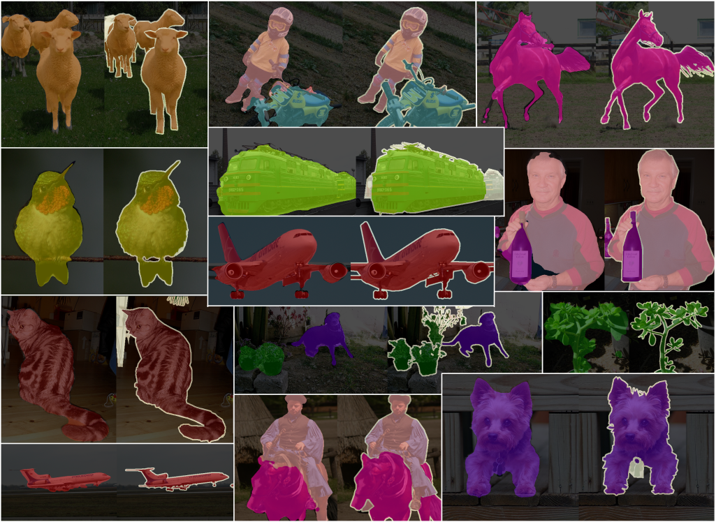
Figure 1: Our segmentation model can produce high-quality semantic masks (left) approaching the ground truth (right) in a single stage of training while using only image-level annotation. No post-processing was applied to these examples.

Attention mechanisms, such Class Activation Maps (CAM) [63], offer a partial solution: they localise the most discriminative regions in the image using only a pre-trained classification network. Such masks, however, are quite coarse – they violate object boundaries, tend to be incomplete for large-scale objects and imprecise for small ones. This is not surprising, since attention maps were not designed for segmentation in the first place. Nevertheless, most methods for weakly supervised segmentation from image labels adopt attention maps (e.g., CAMs) as initial seeds for further refinement. Yet the remarkable progress these methods have achieved – currently reaching more than 80% of fully supervised accuracy [3, 57] – has come along with increased model and training complexity. While early methods consisted of a single stage, i.e. training one network [17, 38, 40, 41], they were soon superseded by more advanced pipelines, employing multiple models, training cycles, and off-the-shelf saliency methods [24, 55, 57, 60].

In this work, we develop an effective single-stage approach for weakly supervised semantic segmentation that streamlines previous multi-stage attempts, and uses neither saliency estimation nor additional data. Our key insight is to enable segmentation-aware training for classification. Consider Fig. 2 depicting typical limitations of attention maps: (i) two areas in local proximity with similar appearance may be assigned different classes, i.e. the semantic labelling may be locally inconsistent; (ii) attention maps tend to be incomplete in terms of covering the whole extent of the object; (iii) while the area of the attention maps dominates for the correct object class, parts of the map may still be mislabelled (i.e. are semantically inaccurate). These observations lead us to define three properties a segmentation-aware training should encompass: (a) local consistency implies that neighbouring pixels with similar appearance share the same label; (b) semantic fidelity is exhibited by models producing segmentation masks that allow for reliable classification decisions (e.g., with good generalisation); (c) completeness means that our model identifies all visible class occurrences in the image. Note that since classification requires only sufficient evidence, CAMs neither ensure completeness nor local consistency.

Using these concepts as our guidelines, we design an approach that significantly outperforms CAMs in terms of segmentation accuracy. First, we propose normalised Global Weighted Pooling, a novel process for computing the classification scores, which enables concurrent training for the segmentation task. Second, we encourage masks to heed appearance cues with Pixel-Adaptive Mask Refinement. These masks are supplied to our model as pseudo ground truth for self-supervised segmentation. Third, to counter the compounding effect of inaccuracies in the pseudo mask annotation (a common problem of self-supervised methods), we introduce a Stochastic Gate that mixes feature representations with varying receptive field sizes. As our experiments demonstrate, the resulting single-stage model offers segmentation quality on par or outperforming the state of the art, while being simple to train and to use.

Figure 2: Typical shortcomings of attention maps (left) vs. pixel-level annotations (right). Our observations of failure modes in attention maps lead to three defining properties of segmentation-aware training from image labels, which we incorporate into our model: semantic fidelity, local consistency, and completeness.

2 Related Work

Methods for weakly supervised semantic segmentation have evolved rapidly from simple single-stage models to more complex ones, employing saliency estimation methods, additional data (e.g., videos), and fully supervised “fine-tuning” (cf. Appendix A).

Single-stage methods.   Following [40], Pinheiro & Collobert [41] used a Multiple Instance Learning (MIL) formulation, but applied a LogSumExp-aggregation of the pixel-level predictions in the output layer to produce the class scores, and refined the segments with image-level priors. Papandreou et al. [38] took an expectation-maximisation (EM) approach, where masks are inferred from intermediate predictions and used as pseudo ground truth. [43] combines top-down attention masks with bottom-up segmentation cues in an end-to-end model using CRF-RNN [62]. The attention-based model [17] allows for joint classification and segmentation training in a cross-domain setting. Despite their simplicity, single-stage models have fallen out of favour, owing to their inferior segmentation accuracy.

Seed and expand.   Kolesnikov & Lampert [28] introduced the idea of expanding high-precision localisation cues, such as CAMs [63], to align with segment boundaries. In this framework, a segmentation network can be trained end-to-end, but the localisation cues are pre-computed from a standalone classification network. Consequently, higher-quality localisation [32] can further improve the segmentation accuracy. Following the seed-and-expand principle, Huang et al. [24] employed a seeded region growing algorithm [1] to encourage larger coverage of the initial localisation seeds.

Erasing.   One common observation with CAMs [63] is their tendency to identify only the most discriminative class evidence. Wei et al. [55] explored the idea of “erasing” these high-confidence areas from the images and re-training the network for classification using the left-over regions to mine for additional cues. Similarly, SeeNet [21] implements erasing using two decoder branches aided by saliency [20]; the first branch removes the peak CAM-response and feeds into the second. To avoid re-training or modifying the decoder structure, Chaudhry et al. [5] iteratively applied an off-the-shelf saliency detector [35] to a progressively erased image in order to accumulate the foreground mask.

Multiple training rounds.   Another line of work trains a chain of segmentation networks, each learning the predictions of its predecessor [27]. Wei et al. [56] sequentially trained three networks in increasing order of task difficulty. Following Khoreva et al. [27], Jing et al. [26] used multiple training rounds and refine intermediate results with GrabCut [42], yet without the use of bounding-box annotations. Similarly, Wang et al. [54] iteratively train a network with the seed-and-expand principle, refine the intermediate results with saliency maps [53], and provide them as supervision to the segmentation network.

Additional data.   Hong et al. [18] sought additional data in videos for training a class-agnostic decoder: at inference time the class-specific attention map has to pass through the decoder individually. More recently, Lee et al. [31] aggregated additional attention maps from videos by merging the detected masks from consecutive frames via warping.

Saliency and further refinement.   Zeng et al. [60] showed that joint training with saliency ground truth significantly improves the mask accuracy. Fan et al. [14] combined the saliency detector of [13] with attention maps to partition the features within each detection window into a segment. To increase the recall of attention maps, Wei et al. [57] added multiple dilation rates in the last layer. Towards the same goal, Lee et al. [30] stochastically selected hidden units and supplied the improved initial seeds to DSRG [24].

Image-level labels only.   In this work we adhere to the early practice of relying only on image-label annotation. Following this setup, Ahn & Kwak [3] modeled the pixel-level affinity distance from initial CAMs and employed a random walk to propagate individual class labels at the pixel level. Instance-aware affinity encoding provides additional benefits [2]. Both methods require training a standalone segmentation network on the masks for the final result – a common practice (e.g., [24, 55, 56, 57]). Shimoda & Yanai [45] proposed to post-refine these masks with a cascade of three additional “difference detection” modules.

In contrast to these works, we develop a competitive alternative with practicality in mind: a single network for weakly supervised segmentation, trained in one cycle.

3 Model

3.1 Overview

Our network model, illustrated in Fig. 3, follows the established design of a fully convolutional segmentation network with a softmax output and skip connections [36]. This allows for a straightforward extension of any segmentation-based network architecture and exploiting pre-trained classification models for parameter pre-conditioning. Inference requires only a single forward pass, analogous to fully supervised segmentation networks. By contrast, however, our model allows to learn for segmentation in a self-supervised fashion from image labels alone.

Figure 3: Architecture overview. Our model shares the design of a segmentation network, but additionally makes use of normalised Global Weighted Pooling (nGWP, Sec. 3.2) and Pixel-Adaptive Mask Refinement (PAMR, Sec. 3.3) to enable self-supervised learning for segmentation from image labels.

We propose three novel components relevant to our task: (i) a new class aggregation function, (ii) a local mask refinement module, and (iii) a stochastic gate. The purpose of the class aggregation function is to leverage segmentation masks for classification decisions, i.e. to provide semantic fidelity as defined earlier. To this end, we develop a normalised Global Weighted Pooling (nGWP) that utilises pixel-level confidence predictions for relative weighting of the corresponding classification scores. Additionally, we incorporate a focal mask penalty into the classification scores to encourage completeness. We discuss these components in more detail in Sec. 3.2. Next, in order to comply with local consistency, we propose Pixel-Adaptive Mask Refinement (PAMR), which revises the coarse mask predictions w.r.t. appearance cues. The updated masks are further used as pseudo ground truth for segmentation, trained jointly along with the classification objective, as we explain in Sec. 3.3. The refined masks produced by PAMR may still contain inaccuracies w.r.t. the ground truth, and self-supervised learning may further compound these errors via overfitting. To alleviate these effects, we devise a Stochastic Gate (SG) that combines a deep feature representation susceptible to this phenomenon with more robust, but less expressive shallow features in a stochastic way. Sec. 3.4 provides further detail.

3.2 Classification scores

CAMs.

It is instructive to briefly review how the class score is normally computed with Global Average Pooling (GAP), since this analysis builds the premise for our aggregation mapping. Let $x_{k,:,:}$ denote one of $K$ feature channels of size $h\times w$ preceding GAP, and $a_{c,:}$ be the parameter vector for class $c$ in the fully connected prediction layer. The class score for class $c$ is then obtained as

$$y^{\text{GAP}}_{c}=\frac{1}{hw}\sum_{k=1}^{K}a_{c,k}\sum_{i,j}x_{k,i,j}.$$ (1)

Next, we can compute the Class Activation Mapping (CAM) [63] for class $c$ as

$$m^{\text{CAM}}_{c,:,:}=\max\bigg{(}0,\sum_{k=1}^{K}a_{c,k}x_{k,:,:}\bigg{)}.$$ (2)

Fig. 4(a) illustrates this process, which we refer to as CAM-GAP. From Eq. 1 we observe that it encourages all pixels in the feature map to identify with the target class. This may disadvantage small segments and increase the reliance of the classifier on the context, which can be undesirable due to a loss in mask precision. Also, as becomes evident from Eq. 2, there are two more issues if we were to adopt CAM-GAP to provide segment cues for learning. First, the mask value is not bounded from above, yet in segmentation we seek a normalised representation (e.g. $\in(0,1)$) that can be interpreted as a confidence by downstream applications. Second, GAP does not encode the notion of pixel-level competition from the underlying segmentation task where each pixel can assume only one class label (i.e. there is no softmax or a related component). We thus argue that CAM-GAP is ill-suited for the segmentation task.

(a)

(b)

Figure 4: The original GAP-CAM architecture 4(a) and our proposed modification, nGWP 4(b). Our analysis of CAMs prompts us to devise an alternative aggregation mapping of class scores, nGWP, which allows to re-use the original classification loss, yet enables joint training for segmentation with substantial improvements in mask quality.

Going beyond CAMs.   To address this, we propose a novel scheme of score aggregation, see Fig. 4(b) for an overview, which allows for seamless integration into existing backbones, yet does not inherit the shortcomings of CAM-GAP. Note that the following discussion is orthogonal to the loss function applied on the final classification scores, which we keep from our baseline model.

Given features $x_{:,:,:}$, we first predict classification scores $y_{:,:,:}$ of size $C\times h\times w$ for each pixel. We then add a background channel (with a constant value) and compute a pixelwise softmax to obtain masks with confidence values $m_{:,:,:}$ – this is a standard block in segmentation. To compute a classification score, we propose normalised Global Weighted Pooling (nGWP), defined as

$$y_{c}^{\text{nGWP}}=\frac{\sum_{i,j}m_{c,i,j}y_{c,i,j}}{\epsilon+\sum_{i^{\prime},j^{\prime}}m_{c,i^{\prime},j^{\prime}}}.$$ (3)

Here, a small $\epsilon>0$ tackles the saturation problem often observed in practice (cf. Appendix B).

As we observe from Eq. 3, nGWP is invariant to the mask size. This may bring advantages for small segments, but lead to inferior recall compared to the more aggressive GAP aggregation. To encourage completeness, we encourage increased mask size for positive classes with a penalty term:

$$y_{c}^{\text{size}}=\log\Big{(}\lambda+\frac{1}{hw}\sum_{i,j}m_{c,i,j}\Big{)}.$$ (4)

The magnitude of this penalty is controlled by a small $\lambda>0$. The logarithmic scale ensures that we incur a large negative value of the penalty only when the mask is near zero. Since we decouple the influence of the class scores (captured by Eq. 3) from that of the mask size (through Eq. 4), we can apply difficulty-aware loss functions. We generalise the penalty term in Eq. 4 to the focal loss [34], used in our final model:

$$y_{c}^{\text{size-focal}}=(1-\bar{m}_{c})^{p}\log(\lambda+\bar{m}_{c}),\>\;\bar{m}_{c}=\tfrac{1}{hw}\sum_{i,j}m_{c,i,j}.$$ (5)

Note that as the mask size approaches zero, $\bar{m}_{c}\rightarrow 0$, the penalty retains its original form, i.e. Eq. 4. However, if the mask is non-zero, $p>0$ discounts the further increase in mask size to focus on the failure cases of near-zero masks. We compute our final classification scores as $y_{c}\equiv y_{c}^{\text{nGWP}}+y_{c}^{\text{size-focal}}$ and use the multi-label soft-margin loss function [39] used in previous work [3, 57] as the classification loss,

$$\mathcal{L}_{\text{cls}}(\mathbf{y},\mathbf{z})=-\frac{1}{C}\sum^{C}_{c=1} z_{c}\log{\bigg{(}\frac{1}{1+e^{-y_{c}}}\bigg{)}}+$$ (6)

$$+(1-z_{c})\log\bigg{(}\frac{e^{-y_{c}}}{1+e^{-y_{c}}}\bigg{)},$$

where $\mathbf{z}$ is a binary vector of ground-truth labels. The loss encourages $y_{c}<0$ for negative classes (i.e. when $z_{c}=0$) and $y_{c}>0$ for positive classes (i.e. when $z_{c}=1$).

3.3 Pixel-adaptive mask refinement

While our classification loss accounts for semantic fidelity and completeness, the task of local mask refinement is to fulfil local consistency: nearby regions sharing the same appearance should be assigned to the same class.

The mapping formalising this idea takes the pixel-level mask predictions $m_{:,:,:}\in(0,1)^{(C+1)\times h\times w}$ (note $+1$ for the background class) and considers the image $I$ to produce refined masks $m_{:,:,:}^{\ast}$. Such a mapping has to be efficient, since we will use it to produce self-supervision for segmentation trained concurrently with the classification objective. Therefore, a naive choice of GrabCut [42] or dense CRFs [29] would slow down the training process.

Figure 5: Concept illustration of Pixel-Adaptive Mask Refinement (PAMR). For each pixel, we compute an affinity kernel measuring its proximity to its neighbours in RGB space. We iteratively apply this kernel to the semantic masks via an adaptive convolution to obtain refined labels.

Instead, our implementation derives from the Pixel-Adaptive Convolution (PAC) [49]. The idea, illustrated in Fig. 5, is to iteratively update pixel label $m_{:,i,j}$ using a convex combination of the labels of its neighbours $\mathcal{N}(i,j)$, i.e. at the $t^{\text{th}}$ iteration we have

$$m^{t}_{:,i,j}=\sum_{(l,n)\in\mathcal{N}(i,j)}\alpha_{i,j,l,n}\cdot m^{t-1}_{:,l,n},$$ (7)

where the pixel-level affinity $\alpha_{i,j,l,n}$ is a function of the image $I$. To compute $\alpha$, we use a kernel function on the pixel intensities $I$,

$$k(I_{i,j},I_{l,n})=-\tfrac{\lvert I_{i,j}-I_{l,n}\rvert}{\sigma_{i,j}^{2}},$$ (8)

where we define $\sigma_{i,j}$ as the standard deviation of the image intensity computed locally for the affinity kernel. We apply a softmax to obtain the final affinity distance $\alpha_{i,j,l,n}$ for each neighbour $(l,n)$ of $(i,j)$, i.e. $\alpha_{i,j,l,n}=e^{\bar{k}(I_{i,j},I_{l,n})}/\sum_{(q,r)\in\mathcal{N}(i,j)}e^{\bar{k}(I_{i,j},I_{q,r}))}$, where $\bar{k}$ is the average affinity value across the RGB channels.

This local refinement, termed Pixel-Adaptive Mask Refinement (PAMR), is implemented as a parameter-free recurrent module, which iteratively updates the labels following Eq. 7. Clearly, the number of required iterations depends on the size and shape of the affinity kernel (e.g. $3\times 3$ in Fig. 5). In practice, we combine multiple $3\times 3$-kernels with varying dilation rates. We study the choice of the affinity structure in more detail in our ablation study (cf. Sec. 4.2). Note that since we do not back-propagate through PAMR, it is always in “evaluation” mode, hence memory-efficient. In practice, one iteration adds less than $1\%$ of the baseline’s GPU footprint, and we empirically found 10 refinement steps to provide a sufficient trade-off between the efficiency and the delivered accuracy boost from PAMR.

Self-supervised segmentation loss.   We generate pseudo ground-truth masks from PAMR by considering pixels with confidence $>60\%$ of the maximum value ($>70\%$ for the background class). Conflicting pixels and pixels with low confidence are ignored by the loss function. We fully discard images for which some of the ground-truth classes do not give rise to any confident pseudo ground-truth pixels. Following the fully supervised case [8], we use pixelwise cross-entropy, but balance the loss distribution across the classes, i.e. the loss for each individual class is normalised w.r.t. the number of corresponding pixels contained in the pseudo ground truth. The intermediate results for segmentation self-supervision at training time are illustrated in Fig. 6.

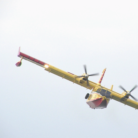
(a) Input

(b) Ground Truth

(c) Prediction

(d) Refinement

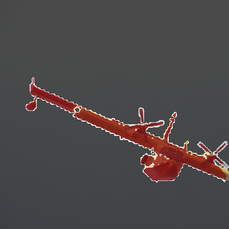
(e) Pseudo GT

Figure 6: Intermediate results at training time. PAMR refines model predictions (middle) by accounting for appearance cues in the image. The revised masks ($4^{\text{th}}$ column) serve as pseudo ground truth, where we use only high-confidence pixels (last column).

3.4 Stochastic gate

In self-supervised learning we expect the model to “average out” inaccuracies (manifested by their irregular nature) in the pseudo ground truth, thereby improving the predictions and thus the pseudo supervision. However, a powerful model may just as well learn to mimic these errors. Strong evidence from previous work indicates that the large receptive field of the deep features enables the model to learn such complex phenomena in segmentation [8, 58, 61].

To counter the compounding effect of the errors in self-supervision, we propose a type of regularisation, referred to as Stochastic Gate (SG). The underlying idea, shown in Fig. 7, is to encourage information sharing between the deep features (with a large receptive field) and “shallow” representation of the preceding layers (with a lower receptive field), by stochastically exchanging these representations, yet maintaining the deep features as the expected value. Formally, let $x^{(d)}$ and $x^{(s)}$ represent the activation in the deep and shallow feature map, respectively (omitting the tensor subscripts for brevity). Applying SG for each pixel at training time is reminiscent of Dropout [48]:

$$\begin{aligned} x^{\text{SG}}=(1-r)\underbrace{\delta[x^{(d)}-\psi x^{(s)}]}_{x^{(\ast)}}+rx^{(s)},\>\text{with}\>r\sim\text{Bern}(\psi),\end{aligned}$$ (9)

where the mixing rate $\psi\in[0,1]$ regulates the proportion of $x^{(\ast)}$ and $x^{(s)}$ in the output tensor. The constant $\delta=1/(1-\psi)$ ensures that $\mathbb{E}[x^{\text{SG}}]=x^{(d)}$. It is easy to show that $x^{(\ast)}\approx x^{(s)}$, encouraged by the stochasticity, implies $x^{(d)}\approx x^{(s)}$, i.e. feature sharing between the deep and shallow representations. At inference time, we deterministically combine the two, now complementary, streams:

$$x^{\text{SG}}=(1-\psi)x^{(d)}+\psi x^{(s)}.$$ (10)

Figure 7: Concept illustration of the Stochastic Gate. All rectangular blocks are tensors of the same size. The baseline model from DeepLabv3+ [8] is shown in red: the output from ASPP is augmented via a skip connection from conv3 and the result, $x^{(d)}$, passes directly through the decoder. Shown in blue, our modification (GCI) infuses global cues extracted from the deep features into the shallow features via AdIN [23]. The enriched shallow and the deep features are then combined using Eq. 9 at training and Eq. 10 at inference time.

Shallow features alone may be too limited in terms of the semantic information they contain. To enrich their representation, yet preserve their original receptive field, we devise Global Cue Injection (GCI) via Adaptive Instance Normalisation (AdIN) [23]. As shown in Fig. 7, we first apply a $1\!\times\!1$ convolution to the deep feature tensor to double the number of channels. Then, we extract two vectors with global information (i.e. without spatial cues) via Global Max Pooling (GMP). Shown as the left (unshaded) and right (shaded) half of the 1D vector after GMP in Fig. 7, let $z^{(a)}$ and $b^{(a)}$ denote two parts of such a representation, which will be shared by each site in a shallow feature channel. We compute the augmented shallow activation $x^{(s)^{\ast}}$ as

$$x^{(s)^{\ast}}=\texttt{ReLU}\Big{(}z^{(a)}\Big{(}\tfrac{x^{(s)}-\mu(x^{(s)})}{\sigma(x^{(s)})}\Big{)}+b^{(a)}\Big{)},$$ (11)

where $\mu(\cdot)$ and $\sigma(\cdot)$ are the mean and the standard deviation of each channel of $x^{(s)}$. The updated activation, $x^{(s)^{\ast}}$, goes through a $1\!\times\!1$-convolution and replaces the original $x^{(s)}$ in Eq. 9 and Eq. 10 in the final form of SG. Following [8], the output from SG then passes through a 3-layer decoder.

4 Experiments

4.1 Setup

Dataset.

Pascal VOC 2012 [12] is an established benchmark for weakly supervised semantic segmentation and contains 20 object categories. Following the standard practice [3, 28, 57], we augment the original VOC training data with an additional image set provided by Hariharan et al. [15]. In total, we use $10\,582$ images with image-level annotation for training and $1449$ images for validation.

Implementation details.   Our model is implemented in PyTorch [39]. We use a WideResNet-38 backbone network [58] provided by [3] (see Appendix F, for experiments with VGG16 [47] and ResNet backbones [16]). We further extend this model to DeepLabv3+ by adding Atrous Spatial Pyramid Pooling (ASPP), a skip connection (with our Stochastic Gate), and the 3-layer decoder [8]. We train our model for $20$ epochs with SGD using weight decay $5\text{\times}{10}^{-4}$ with momentum $0.9$, a constant learning rate of $0.01$ for the new (randomly initialised) modules and $0.001$ for WideResNet-38 parameters, initialised from ImageNet [11] pre-training. We first train our model for 5 epochs using only the classification loss and switch on the self-supervised segmentation loss for the remaining 15 epochs. We use inference with multi-scale inputs [7] and remove masks for classes with classifier confidence $<0.1$.

Data augmentation.   Following common practice [3, 57], we use random rescaling (in the $(0.9,1.0)$ range w.r.t. the original image area), horizontal flipping, colour jittering, and train our model on random crops of size $321\times 321$.

$\downarrow p\hfill/\hfill\lambda\rightarrow$	$0.1$	$0.01$	$0.001$
$0$	$58.8$	$58.9$	$57.4$
$3$	$59.5$	$59.4$	$58.1$
$5$	$60.2$	$59.1$	$57.1$

(a) IoU (val,%) w.r.t. focal mask penalty. We fix $\psi\!=\!0.5$ w/ GCI for SG and use PAMR kernel $[1,2,4,8,12,24]$.

1	2	4	8	12	24	IoU
✓	✓	✓	✓	✓	✓	$59.4$
(no refinement)						$31.8$
✓	✓	✓	✓			$50.6$
✓	✓	✓	✓	✓		$55.7$
✓	3	6	9	✓	16	$57.9$
✓	✓	✓	✓	✓	16	$58.2$

(b) IoU (val,%) w.r.t. Pixel-Adaptive Mask Refinement. We fix $\psi\!=\!0.5$ w/ GCI for SG and set $p\!=\!3,\lambda\!=\!0.01$.

Config	IoU	IoU (+ CRF)
$\psi=0.5$	$59.4$	$62.2$
$\psi=0.5$ w/o GCI	$59.8$	$60.9$
$\psi=0.3$	$59.7$	$62.7$
$\psi=0.3$ w/o GCI	$57.7$	$60.3$
w/o SG	$55.6$	$57.5$
Deterministic Gate	$57.5$	$57.7$

(c) IoU (val,%) w.r.t. the Stochastic Gate. We use $p\!=\!3,\lambda\!=\!0.01$ for the focal penalty and use PAMR kernel $[1,2,4,8,12,24]$.

Table 1: Ablation study on Pascal VOC. We study the role of 1(a) the focal mask penalty, 1(b) the Pixel-Adaptive Mask Refinement, and 1(c) the Stochastic Gate.

4.2 Ablation study

Focal mask penalty.

Following the intuition from [34], the focal mask penalty emphasises training on the current failure cases, i.e. small (large) masks for the classes present (absent) in the image. Recall from Eq. 5 that $\lambda$ controls the penalty magnitude, while $p$ is the discounting rate for better-off image samples. We aim to verify if the “focal” aspect of the mask penalty provides advantages over the baseline penalty (i.e. $p=0$). Table 1(a) summarises the results.

First, we find that the focal version of the mask penalty improves the segmentation quality of the baseline. This improvement, maximised with $p=5$ and $\lambda=0.1$, is tangible, yet comes at a negligible computational cost. Second, we observe that increasing $\lambda$ tends to increase the segmentation accuracy. While changing $\lambda$ from $0.01$ to $0.001$ leads to higher recall on average, it has a detrimental effect on precision. Lastly, we also find that moderate positive values of $p$ in conjunction with CRF refinement lead to more sizeable gains in mask quality: with $p=3,\lambda=0.01$ we achieve $62.2\%$ IoU, whereas the highest IoU with $p=0$ is only $60.5\%$ (reached with $\lambda=0.01$). However, higher values of $p$ do not benefit from CRF processing (e.g. $59.8\%$ with $p=5,\lambda=0.1$). Hence, $p=3$ strikes the best balance between the model accuracy with and without using a CRF. Note that removing the mask penalty, $y_{c}^{\text{size-focal}}$, leads to an expected drop in recall, reaching only $56.6\%$ IoU.

Method	IoU (train,%)	IoU (val,%)
CAM [3] (Our Baseline)	$48.0$	$46.8$
CAM + RW [3]	$58.1$	$57.0$
CAM + RW + CRF [3]	$59.7$	–
CAM + IRN + CRF [2]	$66.5$	–
Ours	$64.7$	$63.4$
Ours + CRF	$66.9$	$65.3$

Table 2: Segmentation quality on Pascal VOC training and validation sets. Here, we use ground-truth image-level labels to remove masks of any false positive classes predicted by our model.

Pixel-Adaptive Mask Refinement (PAMR).   Recall from Sec. 3.3 that PAMR aims to improve the quality of the original coarse masks w.r.t. local consistency to provide self-supervision for segmentation. Here, we verify (i) the importance of PAMR by training our model without the refinement; and (ii) the choice of the kernel structure, i.e. the composition of dilation rates of the $3\times 3$-kernels in PAMR.

The results in Table 1(b) show that PAMR is a crucial component in our self-supervised model, as the segmentation accuracy drops markedly from $59.4\%$ to $31.8\%$ without it. We find further that the size of the kernel also affects the accuracy. This is expected, since small receptive fields (dilations 1-2-4-8 in Table 1(b)) are insufficient to revise the boundaries of the coarse masks that typically exhibit large deviations from the object boundaries. The results with larger receptive fields of the affinity kernel further support this intuition: increasing the dilation of the largest $3\!\times\!3$-kernel to $24$ attains the best mask quality compared to the smaller affinity kernels. Furthermore, we observe that varying the kernel shape does not have such a drastic effect; the change from 1-3-6-9-12-16 to 1-2-4-8-12-16 only leads to small accuracy changes. This is desirable in practice as sensitivity to these minor details would imply that our architecture overfits to particularities in the data [52].

Stochastic Gate (SG).   The intention of the SG, introduced in Sec. 3.4, is to counter overfitting to the errors contained in the pseudo supervision. Here, there are four baselines we aim to verify: (i) disabling SG; (ii) combining $x^{(d)}$ and $x^{(s)}$ deterministically (i.e. $r\equiv\psi$ in Eq. 9); (iii) the role of the Global Cue Injection (GCI); and (iv) the effect of the mixing rate $\psi$. These results are summarised in Table 1(c). Evidently, SG is crucial, since disabling it substantially weakens the mask accuracy (from 59.8% to 55.6% IoU). The stochastic nature of SG is also important: simply summing up $x^{(d)}$ and $x^{(s)}$ (we used $r\equiv\psi=0.5$) yields inferior mask IoU (57.5% vs. 59.8%). In our model comparison with both $\psi=0.5$ and $\psi=0.3$, we find that the model with GCI tends to provide superior results. However, the model without GCI can be as competitive given a particular choice of $\psi$ (e.g., $0.5$). In this case, the model with GCI usually has higher recall, while the model without it has higher precision. Since CRFs tend to increase the precision provided sufficient mask support, the model with GCI should therefore profit more from this refinement. We confirmed this and observed a more sizeable improvement of the model with GCI (59.4 vs. 62.2% IoU). Additionally, we found GCI to deliver more stable results for different $\psi$, which can alleviate parameter fine-tuning in practice.

Method	Backbone	Superv.	Dep.	val	test
Fully supervised
WideResNet38 [58]		$\mathcal{F}$		$80.8$	$82.5$
DeepLabv3+ [8]	Xception-65 [9]	$\mathcal{F}$		–	$87.8$
Multi stage + Saliency
STC [56]	DeepLab [6]	$\mathcal{S},\mathcal{D}$	[25]	$49.8$	$51.2$
SEC [28]	VGG-16	$\mathcal{S},\mathcal{D}$	[46]	$50.7$	$51.7$
Saliency [37]	VGG-16	$\mathcal{S},\mathcal{D}$		$55.7$	$56.7$
DCSP [5]	ResNet-101	$\mathcal{S}$	[35]	$60.8$	$61.9$
RDC [57]	VGG-16	$\mathcal{S}$	[59]	$60.4$	$60.8$
DSRG [24]	ResNet-101	$\mathcal{S}$	[53]	$61.4$	$63.2$
FickleNet [30]	ResNet-101	$\mathcal{S}$	[24]	$64.9$	$65.3$
Frame-to-Frame [31]	VGG-16	$\mathcal{S},\mathcal{D}$	[50, 19, 30]	$63.9$	$65.0$
	ResNet-101			$66.5$	$67.4$
Single stage + Saliency
JointSaliency [60]	DenseNet-169 [22]	$\mathcal{S},\mathcal{D}$		$63.3$	$64.3$
Multi stage
AffinityNet [3]	WideResNet-38	$\mathcal{I}$		$61.7$	$63.7$
IRN [2]	ResNet-50	$\mathcal{I}$		$63.5$	$64.8$
SSDD [45]	WideResNet-38	$\mathcal{I}$	[3]	$64.9$	$65.5$
Single stage
TransferNet [17]	VGG-16	$\mathcal{D}$		$52.1$	$51.2$
WebCrawl [18]	VGG-16	$\mathcal{D}$		$58.1$	$58.7$
EM [38]	VGG-16	$\mathcal{I}$		$38.2$	$39.6$
MIL-LSE [41]	Overfeat [44]	$\mathcal{I}$		$42.0$	$40.6$
CRF-RNN [43]	VGG-16	$\mathcal{I}$		$52.8$	$53.7$
Ours	WideResNet-38	$\mathcal{I}$		$59.7$	$60.5$
Ours + CRF		$\mathcal{I}$		$62.7$	$64.3$

Table 3: Mean IoU (%) on Pascal VOC validation and test. For each method we indicate additional cues used for training beyond image-level labels $\mathcal{I}$, such as saliency detection ($\mathcal{S}$), additional data $(\mathcal{D})$, as well as their dependence on other methods (“Dep.”).

4.3 Comparison to the state of the art

Setup.

Here, our model uses SG with GCI, $\psi=0.3$, the focal penalty with $p=3$ and $\lambda=0.01$, and PAMR with $10$ iterations and a 1-2-4-8-12-24 affinity kernel.

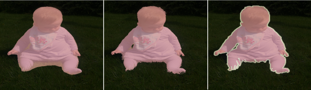
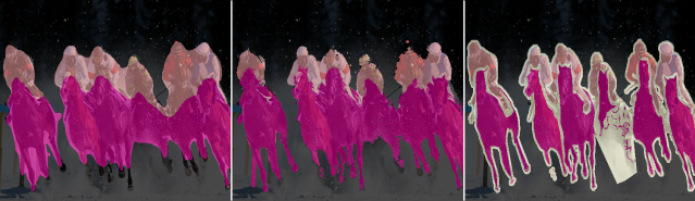
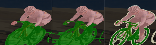
(a) Train

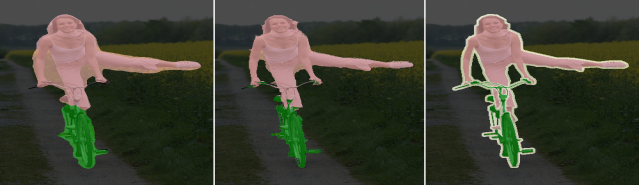
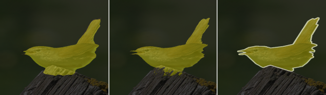
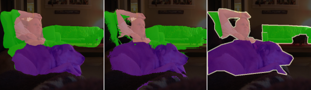
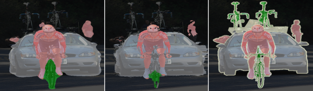
(b) Val

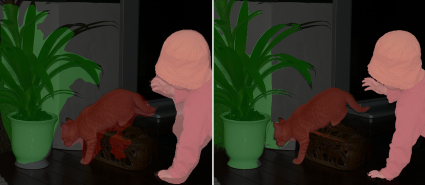
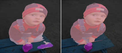
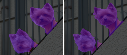
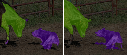
(c) Test

Figure 8: Qualitative results on PASCAL VOC. We show example segmentations from our method (left), the result of CRF post-processing (middle), and the ground truth (right). Our method produces masks of high quality under a variety of challenging conditions.

Mask quality.   Recall that the majority of recent work, e.g. [24, 30, 31, 57], additionally trains a separate fully supervised segmentation network from the pseudo ground truth. To evaluate the quality of such pseudo supervision generated by our model, we use image-level ground-truth labels to remove any masks for classes that are not present in the image (for this experiment only). The results in Table 2 show that using our single-stage mask output as pseudo segmentation labels improves the baseline IoU of CAMs by a staggering $18.9\%$ IoU ($18.5\%$ on validation), and even outperforms recent multi-stage methods [3] by $7.2\%$ IoU and [2] by $0.4\%$ IoU. This is remarkable, since we neither train additional models nor recourse to saliency detection.

Segmentation accuracy.   Table 3 provides a comparative overview w.r.t. the state of the art. Since image-level labels are generally not available at test time, we do not perform any mask pruning here (unlike Table 2). In the setting of image-level supervision, IRN [2] and SSDD [45] are the only methods with higher IoU than ours. Both methods are multi-stage; they are trained in at least three stages. IRNet [2] trains an additional segmentation network on pseudo labels to eventually outperform our method by only $0.5\%$ IoU. Recall that SSDD is essentially a post-processing approach: it refines the masks from AffinityNet [3] (with $63.7\%$ IoU) using an additional network and further employs a cascade of two networks to revise the masks. This strategy improves over our results by only $1.2\%$ IoU, yet at the cost of a considerable increase in model complexity.

Our single-stage method is also competitive with JointSaliency [60], which uses a more powerful backbone [22] and saliency supervision. The recent Frame-to-Frame system [31] is also supervised with saliency and is trained on additional 15K images mined from videos, which requires state-of-the-art optical flow [50]. By contrast, our approach is substantially simpler since we train one network in a single shot. Nevertheless, we surpass a number of multi-stage methods that use additional data and saliency supervision [5, 24, 28, 37, 56]. We significantly improve over previous single-stage methods [38, 41, 43], as well as outperform the single-stage WebCrawl [18], which relies on additional training data and needs multiple forward passes through its class-agnostic decoder. Our model needs neither and infers masks for all classes in one pass.

Note that training a standalone segmentation network on our pseudo labels is a trivial extension, which we omit here in view of our practical goals. However, we still provide these results in the supplemental material (Appendix E), in fact, achieving state of the art in a multi-stage setup as well.

Qualitative analysis.   From the qualitative results in Fig. 8, we observe that our method produces segmentation masks that align well with object boundaries. Our model exhibits good generalisation to challenging scenes with varying object scales and semantic content. Common failure modes of our segmentation network are akin to those of fully supervised methods: segmenting fine-grained details (e.g., bicycle wheels), mislabelling under conditions of occlusions (e.g., leg of the cyclist vs. bicycle), and misleading appearance cues (e.g., low contrast, similar texture).

5 Conclusion

In this work, we proposed a practical approach to weakly supervised semantic segmentation, which comprises a single segmentation network trained in one round. To ensure local consistency, semantic fidelity, and completeness of the segmentation masks, we introduced a new class aggregation function, a local mask refinement module, and a stochastic gate. Our approach is astonishingly effective despite its simplicity. Specifically, it yields segmentation accuracy on par with the state of the art and outperforms a range of recent multi-stage methods relying on additional training data and saliency supervision. We expect that our model can also profit from auxiliary supervision and suit the needs of downstream tasks without considerable deployment effort.

Single-Stage Semantic Segmentation from Image Labels
– Supplemental Material – Nikita Araslanov           Stefan Roth
Department of Computer Science, TU Darmstadt

Appendix A On Training Stages

Table 4 provides a concise overview of previous work on semantic segmentation from image-level labels. As an important practical consideration, we highlight the number of stages used by each method. In this work, we refer to one stage as learning an independent set of model parameters with intermediate results saved offline as input to the next stage. For example, the approach by Ahn et al. [3] comprises three stages: (1) extracting CAMs as seed masks; (2) learning a pixel affinity network to refine these masks; and (3) training a segmentation network on the pseudo labels generated by affinity propagation. Note that three methods [26, 55, 56] also use multiple training cycles (given in parentheses) of the same model, which essentially acts as a multiplier w.r.t. the total number of stages. Finally, we note if a method relies on saliency detection, extra data, or previous frameworks. We observe that predominantly early single-stage methods stand in contrast to the more complex recent multi-stage pipelines. Our approach is single stage and relies neither on previous frameworks, nor on saliency supervision.

Method	Extras	# of Stages	PSR
MIL-FCN ICLR ’15 [40]	–	1	✗
MIL-LSE CVPR ’15 [41]	–	1	✗
EM ICCV ’15 [38]	–	1	✗
TransferNet CVPR ’16 [17]	–	1	✗
SEC ECCV ’16 [28]	$\mathcal{S}$ [46]	2	✗
DCSP ECCV ’17 [5]	$\mathcal{S}$ [35]	1	✗
AdvErasing CVPR ’17 [55]	$\mathcal{S}$ [53]	2 $(\times 3)$	✓
WebCrawl CVPR ’17 [18]	$\mathcal{D}$	1	✗
CRF-RNN CVPR ’17 [43]	–	1	✗
STC TPAMI ’17 [56]	$\mathcal{D}$, $\mathcal{S}$ [25]	3 $(\times 3)$	✓
MCOF CVPR ’18 [54]	$\mathcal{S}$ [54]	2	✗
RDC CVPR ’18 [57]	$\mathcal{S}$ [59]	3	✓
DSRG CVPR ’18 [24]	$\mathcal{S}$ [53]	2	✓
Guided-Att CVPR ’18 [32]	SEC [28]	1+2	✗
SalientInstances ECCV ’18 [14]	$\mathcal{S}$ [13]	2	✓
Affinity CVPR ’18 [3]	–	3	✓
SeeNet NIPS ’18 [21]	$\mathcal{S}$ [20]	2	✓
FickleNet CVPR ’19 [30]	$\mathcal{S}$, DSRG [24]	1+3	✓
JointSaliency ICCV ’19 [60]	$\mathcal{S}$	1	✗
Frame-to-Frame ICCV ’19 [31]	$\mathcal{D}$, $\mathcal{S}$ [19]	2	✓
SSDD ICCV ’19 [45]	Affinity [3]	2+3	✓
IRN CVPR ’19 [2]	–	3	✓
Coarse-to-Fine TIP ’20 [26]	GrabCut [42]	2 $(\times 5)$	✓
Ours	–	1	✗

Table 4: Summary of related work. We analyse the related methods w.r.t. external input (“Extras”), such as saliency detection ($\mathcal{S}$), additional data $(\mathcal{D})$, or their reliance on previous work. We count the number of training stages in the method and note in parentheses if the method uses multiple training cycles of the same models. We also mark methods that additionally train a standalone segmentation network in a (pseudo) fully supervised regime to refine the masks (PSR).

Appendix B Loss Functions

In this section, we take a detailed look at the employed loss functions. Since we compute the classification scores differently from previous work, we also provide additional analysis to justify the form of this novel formulation.

B.1 Classification loss

We use the multi-label soft-margin loss function used in previous work [3, 57] as the classification loss, $\mathcal{L}_{\text{cls}}$. Given model predictions $\mathbf{y}\in\mathbb{R}^{C}$ (cf. Eq. 3 and Eq. 5; see also below) and a binary vector of ground-truth labels $\mathbf{z}\in\{0,1\}^{C}$, we compute the multi-label soft-margin loss [39] as

$$\mathcal{L}_{\text{cls}}(\mathbf{y},\mathbf{z})=-\frac{1}{C}\sum^{C}_{c=1}z_{c}\log{\bigg{(}\frac{1}{1+e^{-y_{c}}}\bigg{)}}+\\ +(1-z_{c})\log\bigg{(}\frac{e^{-y_{c}}}{1+e^{-y_{c}}}\bigg{)}.$$ (12)

As illustrated in Fig. 9, the loss function encourages $y_{c}<0$ for negative classes (i.e. when $z_{c}=0$) and $y_{c}>0$ for positive classes (i.e. when $z_{c}=1$). This observation will be useful for our discussion below.

Recall from Eq. 3 and Eq. 5 that we define our classification score $y_{c}$ as

$$y_{c}=y_{c}^{\text{nGWP}}+y_{c}^{\text{size-focal}}.$$ (13)

For convenience, we re-iterate the definition of the two terms, the normalised Global Weighted Pooling

$$y_{c}^{\text{nGWP}} =\frac{\sum_{i,j}m_{c,i,j}y_{c,i,j}}{\epsilon+\sum_{i^{\prime},j^{\prime}}m_{c,i^{\prime},j^{\prime}}}$$ (14)

and the focal penalty

$$y_{c}^{\text{size-focal}} =(1-\bar{m}_{c})^{p}\log(\lambda+\bar{m}_{c}),$$ (15)

$$\text{with}\qquad\bar{m}_{c} =\frac{1}{hw}\sum_{i,j}m_{c,i,j}.$$ (16)

Note that $y_{c,i,j}$ in Eq. 14 refers to pixel site $(i,j)$ on the score map of class $c$, whereas $y_{c}$ in Eq. 13 is the aggregated score for class $c$. We compute the class confidence $m_{:,i,j}$ for site $(i,j)$ using a softmax on $y_{:,i,j}$, where we include an additional background channel $y_{0,i,j}$. We fix $y_{0,:,:}\equiv 1$ throughout our experiments.

Figure 9: Soft-margin classification loss. The loss encourages $y_{c}>0$ for positive classes and $y_{c}<0$ for negative classes. The function exhibits saturation regions: as $y_{c}\rightarrow\infty$ for positive classes, the associated loss (shown in blue) approaches $0$. Conversely, the loss for negative classes, shown in red, approaches $0$, as $y_{c}\rightarrow-\infty$.

The use of hyperparameter $\epsilon>0$ in the definition of Eq. 14 may look rather arbitrary and redundant at first. In the analysis below, we show that in fact it serves multiple purposes:

1. Numerical stability. First, using $\epsilon>0$ prevents division by zero for saturated scores, i.e. where $\sum_{i^{\prime},j^{\prime}}m_{c,i^{\prime},j^{\prime}}=0$ for some $c$ in the denominator of Eq. 14, which can happen (approximately) in the course of training for negative classes.

   Secondly, $\epsilon>0$ resolves discontinuity issues. Observe that

   $$\lim_{m_{c,:,:}\rightarrow 0}\>\frac{\sum_{i,j}m_{c,i,j}y_{c,i,j}}{\epsilon+\sum_{i^{\prime},j^{\prime}}m_{c,i^{\prime},j^{\prime}}}=0,$$ (17)

   i.e. $y_{c}^{\text{nGWP}}\approx 0$ for negative classes and positive $\epsilon$.

   However, with $\epsilon=0$ the nGWP term in Eq. 14 is not continuous at 0, which in practice may result in unstable training when $\sum_{i,j}m_{c,i,j}\approx 0$ for some $c$. One exception, unlikely to occur in practice, is when $y_{c,i,j}=y_{c,k,l}=d$ for all $(i,j)$ and $(k,l)$. Then,

   $$\lim_{m_{c,:,:}\rightarrow 0}\frac{\sum_{i,j}m_{c,i,j}y_{c,i,j}}{\sum_{i^{\prime},j^{\prime}}m_{c,i^{\prime},j^{\prime}}}=\\ =\lim_{m_{c,:,:}\rightarrow 0}\frac{d\sum_{i,j}m_{c,i,j}}{\sum_{i^{\prime},j^{\prime}}m_{c,i^{\prime},j^{\prime}}}=d.$$ (18)

   In the case of more practical relevance, i.e. when $y_{c,i,j}\neq y_{c,k,l}$ for some $(i,j)\neq(k,l)$, the limit does not exist, as the following lemma shows. With some abuse of notation, we here write $m_{i}$ and $y_{i}$ to refer to the confidence and the score values of class $c$ at pixel site $i$, respectively.

   Lemma 1.

   Let $\epsilon=0$ in Eq. 14 and suppose there exist $k$ and $l$ such that $y_{k}\neq y_{l}$. Then, the corresponding limit

   $$\lim_{m_{i}\rightarrow 0,\forall i}\frac{\sum_{i}m_{i}y_{i}}{\sum_{i^{\prime}}m_{i^{\prime}}}$$ (19)

   does not exist.

   Proof.

   Let $m_{k}(t)=t$ and $m_{i}(t)=0$ for $i\neq k$. Then,

   $$\lim_{m_{i}\rightarrow 0,\forall i}\frac{\sum_{i}m_{i}y_{i}}{\sum_{i^{\prime}}m_{i^{\prime}}}=\lim_{t\rightarrow 0}\frac{ty_{k}}{t}=y_{k}.$$

   On the other hand, if we let $m_{l}(t)=t$ and $m_{i}(t)=0$ for $i\neq l$, we obtain

   $$\lim_{m_{i}\rightarrow 0,\forall i}\frac{\sum_{i}m_{i}y_{i}}{\sum_{i^{\prime}}m_{i^{\prime}}}=\lim_{t\rightarrow 0}\frac{ty_{l}}{t}=y_{l}.$$

   Since $y_{k}\neq y_{l}$ by our assumption, we have now found two paths of the multivariable limit in Eq. 19, which evaluate to different values. Therefore, the limit in Eq. 19 is not unique, i.e. does not exist (stewart12, Ch. 14.2). ∎

2. Emphasis on the focal penalty. For negative classes, it is not sensible to give meaningful relative weightings of the pixels for nGWP in Eq. 14; we seek such a relative weighting of different pixels only for positive classes. At training time we would thus like to minimise the class scores for negative classes uniformly for all pixel sites. Empirically, we observed that with $\epsilon>0$ the focal penalty term, which encourages this behaviour, contributes more significantly to the score of the negative classes than the nGWP term, which relies on relative pixel weighting.

   Method	bg	aero	bike	bird	boat	bot.	bus	car	cat	chair	cow	tab.	dog	horse	mbk	per.	plant	sheep	sofa	train	tv	mean
   Multi stage
   SEC∗ [28]	$82.4$	$62.9$	$26.4$	$61.6$	$27.6$	$38.1$	$66.6$	$62.7$	$75.2$	$22.1$	$53.5$	$28.3$	$65.8$	$57.8$	$62.3$	$52.5$	$32.5$	$62.6$	$32.1$	$45.4$	$45.3$	$50.7$
   AdvErasing∗ [55]	$83.4$	$71.1$	$30.5$	$72.9$	$41.6$	$55.9$	$63.1$	$60.2$	$74.0$	$18.0$	$66.5$	$32.4$	$71.7$	$56.3$	$64.8$	$52.4$	$37.4$	$69.1$	$31.4$	$58.9$	$43.9$	$55.0$
   RDC∗ [57]	$89.4$	$85.6$	$34.6$	$75.8$	$61.9$	$65.8$	$67.1$	$73.3$	$80.2$	$15.1$	$69.9$	$8.1$	$75.0$	$68.4$	$70.9$	$71.5$	$32.6$	$74.9$	$24.8$	$73.2$	$50.8$	$60.4$
   FickleNet∗ [30]	$88.1$	$75.0$	$31.3$	$75.7$	$48.8$	$60.1$	$80.0$	$72.7$	$79.6$	$25.7$	$67.3$	$42.2$	$77.1$	$67.5$	$65.4$	$69.2$	$42.2$	$74.1$	$34.2$	$53.7$	$54.7$	$61.2$
   AffinityNet [3]	$88.2$	$68.2$	$30.6$	$81.1$	$49.6$	$61.0$	$77.8$	$66.1$	$75.1$	$29.0$	$66.0$	$40.2$	$80.4$	$62.0$	$70.4$	$73.7$	$42.5$	$70.7$	$42.5$	$68.1$	$51.6$	$61.7$
   FickleNet∗,† [30]	$89.5$	$76.6$	$32.6$	$74.6$	$51.5$	$71.1$	$83.4$	$74.4$	$83.6$	$24.1$	$73.4$	$47.4$	$78.2$	$74.0$	$68.8$	$73.2$	$47.8$	$79.9$	$37.0$	$57.3$	$64.6$	$64.9$
   SSDD [45]	$89.0$	$62.5$	$28.9$	$83.7$	$52.9$	$59.5$	$77.6$	$73.7$	$87.0$	$34.0$	$83.7$	$47.6$	$84.1$	$77.0$	$73.9$	$69.6$	$29.8$	$84.0$	$43.2$	$68.0$	$53.4$	$64.9$
   Single stage
   TransferNet∗ [17]	$85.3$	$68.5$	$26.4$	$69.8$	$36.7$	$49.1$	$68.4$	$55.8$	$77.3$	$6.2$	$75.2$	$14.3$	$69.8$	$71.5$	$61.1$	$31.9$	$25.5$	$74.6$	$33.8$	$49.6$	$43.7$	$52.1$
   CRF-RNN [43]	$85.8$	$65.2$	$29.4$	$63.8$	$31.2$	$37.2$	$69.6$	$64.3$	$76.2$	$21.4$	$56.3$	$29.8$	$68.2$	$60.6$	$66.2$	$55.8$	$30.8$	$66.1$	$34.9$	$48.8$	$47.1$	$52.8$
   WebCrawl∗ [18]	$87.0$	$69.3$	$32.2$	$70.2$	$31.2$	$58.4$	$73.6$	$68.5$	$76.5$	$26.8$	$63.8$	$29.1$	$73.5$	$69.5$	$66.5$	$70.4$	$46.8$	$72.1$	$27.3$	$57.4$	$50.2$	$58.1$
   Ours	$87.0$	$63.4$	$33.1$	$64.5$	$47.4$	$63.2$	$70.2$	$59.2$	$76.9$	$27.3$	$67.1$	$29.8$	$77.0$	$67.2$	$64.0$	$72.4$	$46.5$	$67.6$	$38.1$	$68.2$	$63.6$	$59.7$
   Ours + CRF	$88.7$	$70.4$	$35.1$	$75.7$	$51.9$	$65.8$	$71.9$	$64.2$	$81.1$	$30.8$	$73.3$	$28.1$	$81.6$	$69.1$	$62.6$	$74.8$	$48.6$	$71.0$	$40.1$	$68.5$	$64.3$	$62.7$
   Methods marked with $(^{\ast})$ use saliency detectors or additional data, or both (see Sec. 2). $(^{\dagger})$ denotes a ResNet-101 backbone.

   Table 5: Per-class IoU (%) comparison on Pascal VOC 2012, validation set.

   Method	bg	aero	bike	bird	boat	bot.	bus	car	cat	chair	cow	tab.	dog	horse	mbk	per.	plant	sheep	sofa	train	tv	mean
   Multi stage
   SEC∗ [28]	$83.5$	$56.4$	$28.5$	$64.1$	$23.6$	$46.5$	$70.6$	$58.5$	$71.3$	$23.2$	$54.0$	$28.0$	$68.1$	$62.1$	$70.0$	$55.0$	$38.4$	$58.0$	$39.9$	$38.4$	$48.3$	$51.7$
   FickleNet∗ [30]	$88.5$	$73.7$	$32.4$	$72.0$	$38.0$	$62.8$	$77.4$	$74.4$	$78.6$	$22.3$	$67.5$	$50.2$	$74.5$	$72.1$	$77.3$	$68.8$	$52.5$	$74.8$	$41.5$	$45.5$	$55.4$	$61.9$
   AffinityNet [3]	$89.1$	$70.6$	$31.6$	$77.2$	$42.2$	$68.9$	$79.1$	$66.5$	$74.9$	$29.6$	$68.7$	$56.1$	$82.1$	$64.8$	$78.6$	$73.5$	$50.8$	$70.7$	$47.7$	$63.9$	$51.1$	$63.7$
   FickleNet∗,† [30]	$89.8$	$78.3$	$34.1$	$73.4$	$41.2$	$67.2$	$81.0$	$77.3$	$81.2$	$29.1$	$72.4$	$47.2$	$76.8$	$76.5$	$76.1$	$72.9$	$56.5$	$82.9$	$43.6$	$48.7$	$64.7$	$65.3$
   SSDD [45]	$89.5$	$71.8$	$31.4$	$79.3$	$47.3$	$64.2$	$79.9$	$74.6$	$84.9$	$30.8$	$73.5$	$58.2$	$82.7$	$73.4$	$76.4$	$69.9$	$37.4$	$80.5$	$54.5$	$65.7$	$50.3$	$65.5$
   Single stage
   TransferNet∗ [17]	$85.7$	$70.1$	$27.8$	$73.7$	$37.3$	$44.8$	$71.4$	$53.8$	$73.0$	$6.7$	$62.9$	$12.4$	$68.4$	$73.7$	$65.9$	$27.9$	$23.5$	$72.3$	$38.9$	$45.9$	$39.2$	$51.2$
   CRF-RNN [43]	$85.7$	$58.8$	$30.5$	$67.6$	$24.7$	$44.7$	$74.8$	$61.8$	$73.7$	$22.9$	$57.4$	$27.5$	$71.3$	$64.8$	$72.4$	$57.3$	$37.3$	$60.4$	$42.8$	$42.2$	$50.6$	$53.7$
   WebCrawl∗ [18]	$87.2$	$63.9$	$32.8$	$72.4$	$26.7$	$64.0$	$72.1$	$70.5$	$77.8$	$23.9$	$63.6$	$32.1$	$77.2$	$75.3$	$76.2$	$71.5$	$45.0$	$68.8$	$35.5$	$46.2$	$49.3$	$58.7$
   Ours	$87.4$	$63.6$	$34.7$	$59.9$	$40.1$	$63.3$	$70.2$	$56.5$	$71.4$	$29.0$	$71.0$	$38.3$	$76.7$	$73.2$	$70.5$	$71.6$	$55.0$	$66.3$	$47.0$	$63.5$	$60.3$	$60.5$
   Ours + CRF	$89.2$	$73.4$	$37.3$	$68.3$	$45.8$	$68.0$	$72.7$	$64.1$	$74.1$	$32.9$	$74.9$	$39.2$	$81.3$	$74.6$	$72.6$	$75.4$	$58.1$	$71.0$	$48.7$	$67.7$	$60.1$	$64.3$
   Methods marked with $(^{\ast})$ use saliency detectors or additional data, or both (see Sec. 2). $(^{\dagger})$ denotes a ResNet-101 backbone.

   Table 6: Per-class IoU (%) comparison on Pascal VOC 2012, test set.

3. Negative class debiasing. Negative classes dominate in the label set of Pascal VOC, i.e. each image sample depicts only few categories. The gradient of the loss function from Eq. 12 vanishes for positive classes with $y_{c}\rightarrow\infty$ and negative classes with $y_{c}\rightarrow-\infty$. However, in our preliminary experiments with GAP-CAM, and later with nGWP with $\epsilon=0$ in Eq. 14, we observed that further iterations continued to decrease the scores for the negative classes in regions in which the loss is near-saturated, while the $y_{c}$ of positive classes increased only marginally. This may indicate a strong inductive bias towards negative classes, which might be undesirable for real-world deployment.

   Assuming $\epsilon>0$ and $\sum_{i^{\prime},j^{\prime}}m_{c,i^{\prime},j^{\prime}}\neq 0$, we observe that,

   $$\frac{\sum_{i,j}m_{c,i,j}y_{c,i,j}}{\epsilon+\sum_{i^{\prime},j^{\prime}}m_{c,i^{\prime},j^{\prime}}}>\frac{\sum_{i,j}m_{c,i,j}y_{c,i,j}}{\sum_{i^{\prime},j^{\prime}}m_{c,i^{\prime},j^{\prime}}}$$ (20)

   when $y_{c,:,:}<0$, which is the case for saturated negative classes. Recall further that the use of the constant background score (fixed to $1$) implies that $m_{c,i,j}\rightarrow 0$ as $y_{c,i,j}\rightarrow-\infty$. Since the RHS is the convex combination of $y_{c,i,j}$’s, its minimum is $\min(\{y_{c,i,j}\}_{i,j})$. Therefore, the RHS is unbounded from below as $y_{c,i,j}\rightarrow-\infty$, hence the $y_{c,i,j}$ keep getting pushed down for negative classes. By contrast, the LHS has a defined limit of $0$ as $m_{c,i,j}\rightarrow 0$ (see Eq. 17), which is undesirable as the score for a negative class. This is because a finite (i.e. larger) $m_{c,i,j}$ yields a negative, thus smaller value of the classification score, which we are trying to minimise in this case. Therefore, $\epsilon>0$ will encourage SGD to pull the negative scores away from the saturation areas by pushing the $\sum_{i,j}m_{c,i,j}$ away from zero.

In summary, for negative classes $\epsilon$ improves numerical stability and emphasises the focal penalty while leveraging nGWP to alleviate the negative class bias. For positive classes, the effect of $\epsilon$ is negligible, since $\epsilon\ll\sum_{i,j}m_{c,i,j}$ in this case. We set $\epsilon=1$ in all our experiments.

B.2 Segmentation loss

For the segmentation loss w.r.t. the pseudo ground truth, we use a weighted cross-entropy defined for each pixel site $(i,j)$ as

$$\mathcal{L}_{\text{seg},i,j}=-q_{c}\log m_{c,i,j},$$ (21)

where $c$ is the label in the pseudo ground-truth mask. The balancing class weight $q_{c}$ accounts for the fact that the pseudo ground truth may contain a different amount of pixel supervision for each class:

$$q_{c}=\frac{M_{b,\text{total}}-M_{b,c}}{1+M_{b,\text{total}}},$$ (22)

where $M_{b,\text{total}}$ and $M_{b,c}$ are the total and class-specific number of pixels for supervision in the pseudo ground-truth mask, respectively; $b$ indexes the sample in a batch; and $1$ in the denominator serves for numerical stability. The aggregated segmentation loss $\mathcal{L}_{\text{seg}}$ is a weighted mean over the samples in a batch, i.e.

$$\mathcal{L}_{\text{seg}}=\frac{1}{\sum_{b^{\prime}}M_{b^{\prime},\text{total}}}\frac{1}{hw}\sum_{b}M_{b,\text{total}}\sum_{i,j}\mathcal{L}_{\text{seg},i,j}.$$ (23)

Appendix C Quantitative Analysis

We list the per-class segmentation accuracy on Pascal VOC validation and training in Tables 5 and 6. We first observe that none of previous methods, including the state of the art [3, 30, 45], outperforms other pipelines on all class categories. For example FickleNet [30], based on a ResNet-101 backbone, reaches top segmentation accuracy only for classes “bottle”, “bus”, “car”, and “tv”. SSDD [45] has the highest mean IoU, but is inferior to other methods on 10 out of 21 classes. Our single-stage method compares favourably even to the multi-stage approaches that rely on saliency supervision or additional data. For example, we improve over the more complex AffinityNet [3] that trains a deep network to predict pixel-level affinity distance from CAMs and then further trains a segmentation network in a (pseudo) fully supervised regime. The best single-stage method from previous work, CRF-RNN [43], trained using only the image-level annotation we consider in this work, reaches $52.8\%$ and $53.7\%$ IoU on the validation and test sets. We substantially boost this result, by $9.9\%$ and $10.6\%$ points, respectively, and attain new a state-of-the-art mask accuracy overall on classes “bike”, “person”, and “plant”.

Appendix D Ablation Study: PAMR Iterations

We empirically verify the number of iterations used in PAMR, which we set to $10$ in our main ablation study. Table 7 reports the results with higher and fewer number of iterations. We observe that using only few PAMR iterations decreases the mask quality. On the other hand, the benefits of PAMR diminishes if we increase the number of iterations further. $10$ iterations appears to strike a good balance between the computational expense and the obtained segmentation accuracy.

Additionally, we visualise semantic masks produced at intermediate iterations from our PAMR module in Fig. 10. The initial masks produced by our segmentation model in the early stages of training exhibit coarse boundaries. PAMR mitigates this shortcoming by virtue of exploiting visual cues with pixel-adaptive convolutions. Our model then uses the revised masks to generate pseudo ground-truth for self-supervised segmentation.

Number of iterations	IoU	IoU w/ CRF
5	$59.1$	$59.0$
10	$59.4$	$62.2$
15	$59.0$	$61.6$

Table 7: Effect of the iteration number in PAMR. We train our model with the iteration number in the PAMR module fixed to a pre-defined value. We report the IoU (%) with and without CRF refinement on Pascal VOC validation.

Appendix E Pseudo Labels

The last-stage training of a segmentation network is agnostic to the process of pseudo-label generation; it is the quality of the pseudo labels and the ease of obtaining them that matters.

Method	Backbone	Supervision	val	test
Fully supervised
WideResNet38 [58]		$\mathcal{F}$	$80.8$	$82.5$
DeepLabv3+ [8]	Xception-65 [9]	$\mathcal{F}$	–	$87.8$
Multi stage + Saliency
FickleNet [30]	ResNet-101	$\mathcal{S}$	$64.9$	$65.3$
Frame-to-Frame [31]	VGG-16	$\mathcal{S},\mathcal{D}$	$63.9$	$65.0$
	ResNet-101		$66.5$	$67.4$
Single stage + Saliency
JointSaliency [60]	DenseNet-169 [22]	$\mathcal{S},\mathcal{D}$	$63.3$	$64.3$
Multi stage
AffinityNet [3]	WideResNet-38	$\mathcal{I}$	$61.7$	$63.7$
IRN [2]	ResNet-50	$\mathcal{I}$	$63.5$	$64.8$
SSDD [45]	WideResNet-38	$\mathcal{I}$	$64.9$	$65.5$
Two stage
Ours + DeepLabv3+	ResNet-101	$\mathcal{I}$	$65.7$	$66.6$
Ours + DeepLabv3+	Xception-65	$\mathcal{I}$	$66.8$	$67.3$

Table 8: Mean IoU (%) on Pascal VOC validation and test sets. We train DeepLabv3+ in a fully supervised regime on pseudo ground truth obtained from our method (with CRF refinement). Under equivalent level of supervision, our two-stage approach outperforms the previous state of the art, trained in three or more stages and performs on par with other multi-stage frameworks relying on additional data and saliency detection [31].

Although we intentionally omitted the common practice of training a standalone network on our pseudo labels, we show that, in fact, we can achieve state-of-the-art results in a multi-stage setting as well.

We use our pseudo labels on the train split of Pascal VOC (see Table 2) and train a segmentation model DeepLabv3+ [8] in a fully supervised fashion. Table 8 summarises the results. We observe that the resulting simple two-stage pipeline outperforms other multi-stage frameworks under the same image-level supervision. Remarkably, our method even attains the mask accuracy of Frame-to-Frame [31], which not only utilises saliency detectors, but also relies on additional data (15K extra) and sophisticated network models (e.g. PWC-Net [46], FickleNet [30]).

	Baseline (CAM)			Ours
Backbone	w/o CRF	+ CRF		w/o CRF	+ CRF
VGG16	$41.2$	$38.0$		$55.9$	$56.6$
ResNet-50	$43.7$	$43.5$		$60.4$	$64.1$
ResNet-101	$46.2$	$45.2$		$62.9$	$66.2$
WideResNet-38	$44.9$	$45.2$		$63.1$	$65.8$
Mean	$44.0$	$43.0$		$60.6$	$63.2$

Table 9: Segmentation quality (IoU, %) on Pascal VOC validation. We use ground-truth image-level labels to remove false positive classes from the masks to decouple the segmentation quality from the accuracy of the classifier.

Appendix F Exchanging Backbones

Here we confirm that our segmentation method generalises well to other backbone architectures. We choose VGG16 [47], ResNet-50 and ResNet-101 [16] – all widely used network architectures – as a drop-in alternative to WideResNet-38 [58], which we use for all other experiments. We train these models on $448\times 448$ image crops using the same data augmentation as before. We use multi-scale inference with image sides varying by factors $1.0$, $0.75$, $1.25$, $1.5$. These scales are slightly different from the ones we used in the main experiments, which we found to slightly improve the IoU on average. We re-evaluate our WideResNet-38 on the same scales to make the results from different backbones compatible. Motivated to measure the segmentation accuracy alone, we report validation IoU on the masks with the false positives removed using ground-truth labels. Table 9 summarises the results.

The results show a clear improvement over the CAM baseline for all backbones: the average improvement without CRF post-processing is $16.6\%$ IoU and $20.2\%$ IoU with CRF refinement.

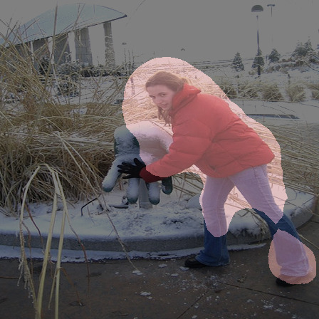
(a) Prediction

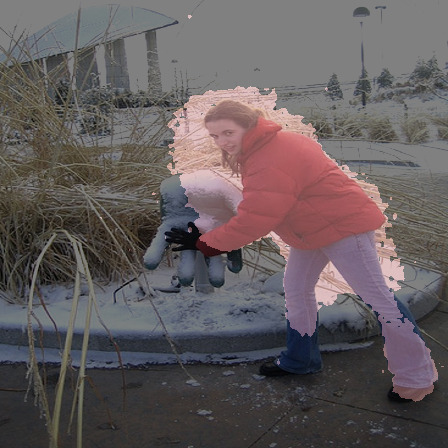
(b) Iteration 1

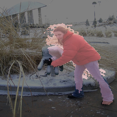
(c) Iteration 3

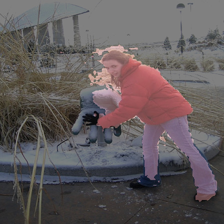
(d) Iteration 5

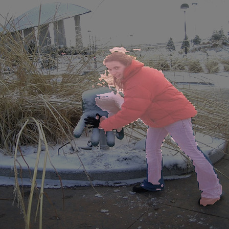
(e) Iteration 7

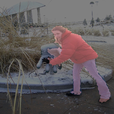
(f) Iteration 10

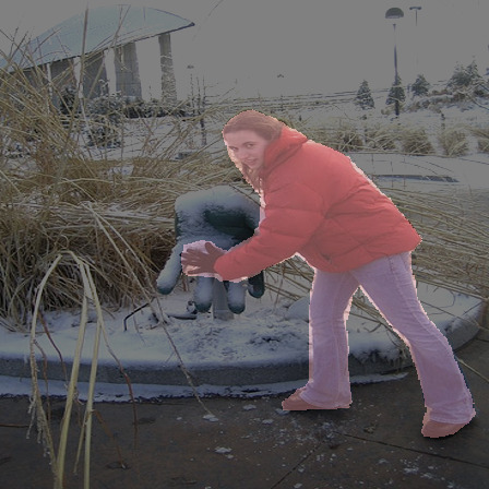
(g) Ground Truth

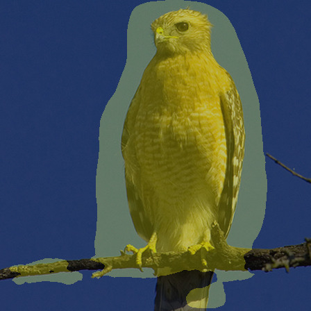
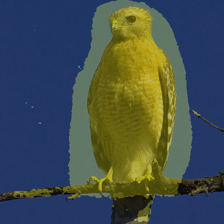
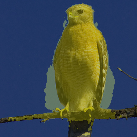
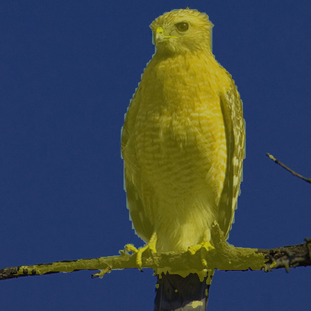
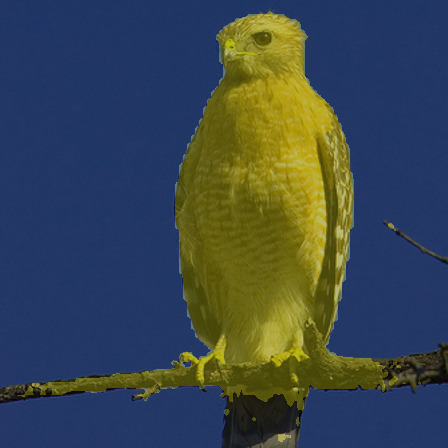
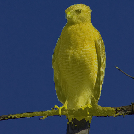
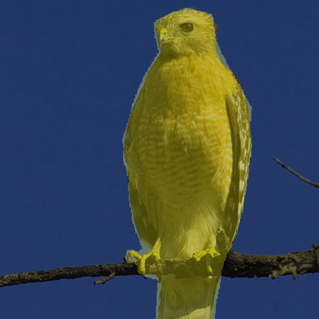
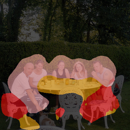
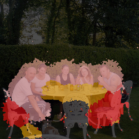
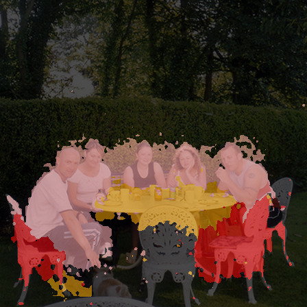
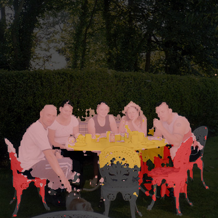
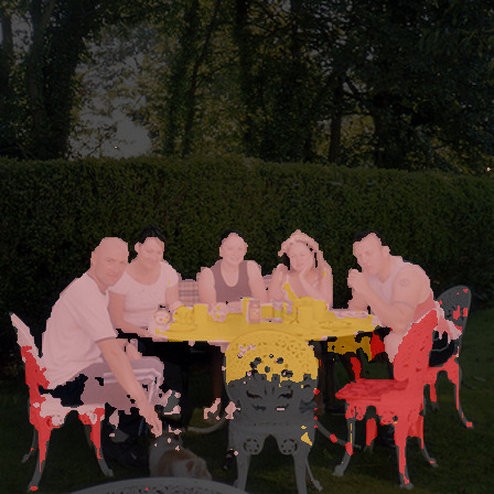
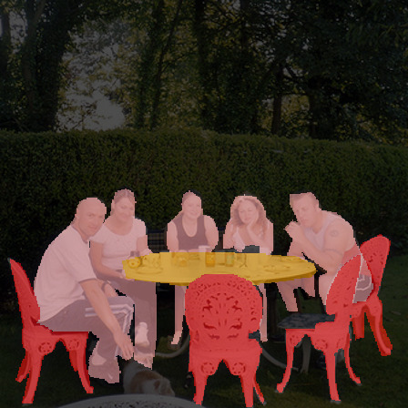
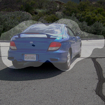
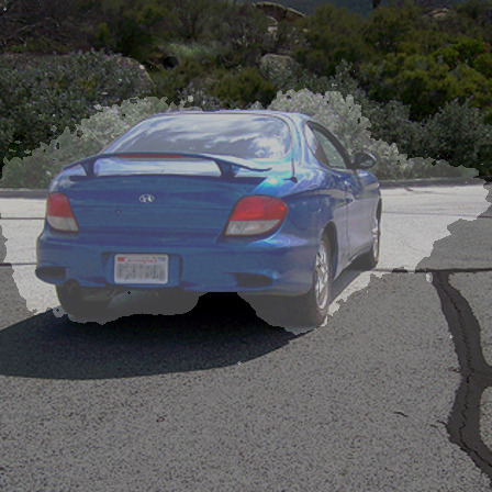
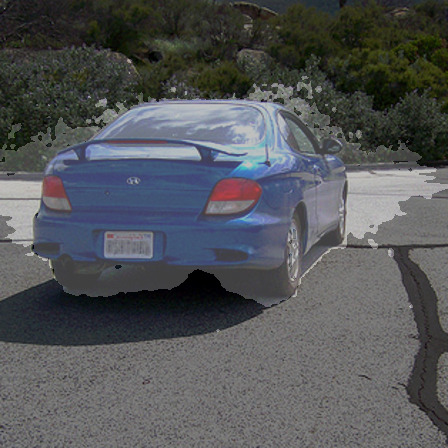
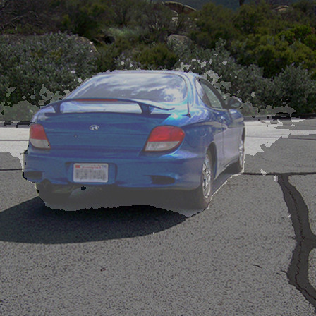
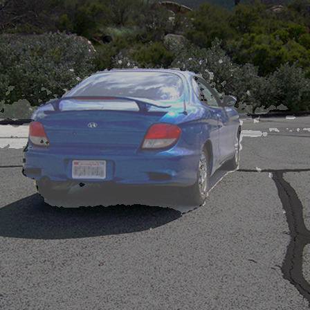
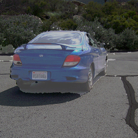
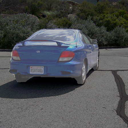
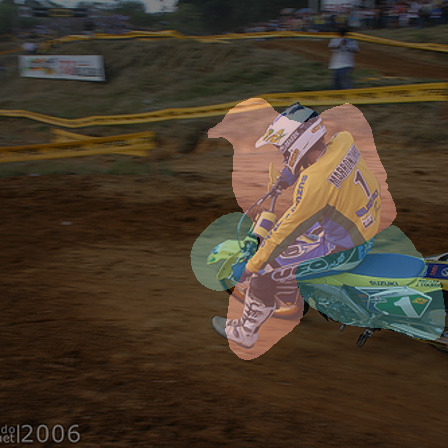
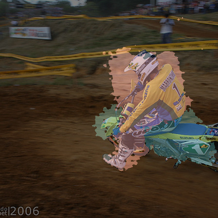
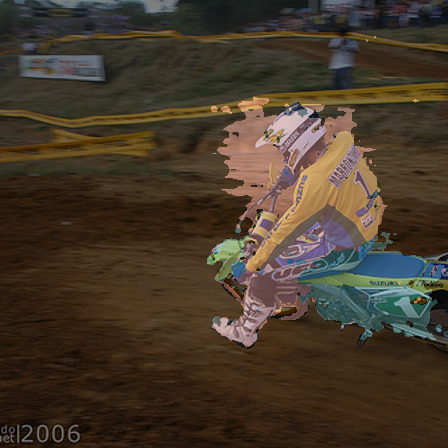
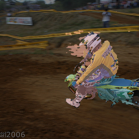
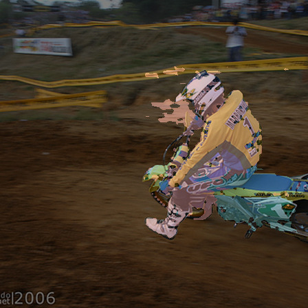
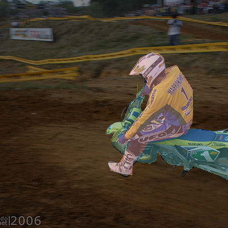
Figure 10: Visualisation of PAMR iterations. The initial model predictions suffer from local inconsistency: mask boundaries do not align with available visual cues. Our PAMR module iteratively revises the masks to alleviate this problem. Our model uses the mask from the last iteration for self-supervision.

ieee_fullname egbib_supp

References

- [1] Rolf Adams and Leanne Bischof. Seeded region growing. IEEE Trans. Pattern Anal. Mach. Intell., 16(6):641–647, 1994.
- [2] Jiwoon Ahn, Sunghyun Cho, and Suha Kwak. Weakly supervised learning of instance segmentation with inter-pixel relations. In CVPR, pages 2209–2218, 2019.
- [3] Jiwoon Ahn and Suha Kwak. Learning pixel-level semantic affinity with image-level supervision for weakly supervised semantic segmentation. In CVPR, pages 4981–4990, 2018.
- [4] Amy Bearman, Olga Russakovsky, Vittorio Ferrari, and Li Fei-Fei. What’s the point: Semantic segmentation with point supervision. In ECCV, pages 549–565, 2016.
- [5] Arslan Chaudhry, Puneet Kumar Dokania, and Philip H. S. Torr. Discovering class-specific pixels for weakly-supervised semantic segmentation. In BMVC, 2017.
- [6] Liang-Chieh Chen, George Papandreou, Iasonas Kokkinos, Kevin Murphy, and Alan L. Yuille. DeepLab: Semantic image segmentation with deep convolutional nets, atrous convolution, and fully connected CRFs. IEEE Trans. Pattern Anal. Mach. Intell., 40(4):834–848, 2017.
- [7] Liang-Chieh Chen, Yi Yang, Jiang Wang, Wei Xu, and Alan L. Yuille. Attention to scale: Scale-aware semantic image segmentation. In CVPR, pages 3640–3649, 2016.
- [8] Liang-Chieh Chen, Yukun Zhu, George Papandreou, Florian Schroff, and Hartwig Adam. Encoder-decoder with atrous separable convolution for semantic image segmentation. In ECCV, pages 833–851, 2018.
- [9] François Chollet. Xception: Deep learning with depthwise separable convolutions. In CVPR, pages 1800–1807, 2017.
- [10] Jifeng Dai, Kaiming He, and Jian Sun. BoxSup: Exploiting bounding boxes to supervise convolutional networks for semantic segmentation. In CVPR, pages 1635–1643, 2015.
- [11] Jia Deng, Wei Dong, Richard Socher, Li-Jia Li, Kai Li, and Li Fei-Fei. ImageNet: A large-scale hierarchical image database. In CVPR, pages 248–255, 2009.
- [12] Mark Everingham, Luc J. Van Gool, Christopher K. I. Williams, John M. Winn, and Andrew Zisserman. The Pascal Visual Object Classes (VOC) Challenge. Int. J. Comp. Vis., 88(2):303–338, 2010.
- [13] Ruochen Fan, Ming-Ming Cheng, Qibin Hou, Tai-Jiang Mu, Jingdong Wang, and Shi-Min Hu. S4net: Single stage salient-instance segmentation. In CVPR, pages 6103–6112, 2019.
- [14] Ruochen Fan, Qibin Hou, Ming-Ming Cheng, Gang Yu, Ralph R. Martin, and Shi-Min Hu. Associating inter-image salient instances for weakly supervised semantic segmentation. In ECCV, pages 371–388, 2018.
- [15] Bharath Hariharan, Pablo Arbelaez, Lubomir D. Bourdev, Subhransu Maji, and Jitendra Malik. Semantic contours from inverse detectors. In ICCV, pages 991–998, 2011.
- [16] Kaiming He, Xiangyu Zhang, Shaoqing Ren, and Jian Sun. Deep residual learning for image recognition. In CVPR, pages 770–778, 2016.
- [17] Seunghoon Hong, Junhyuk Oh, Honglak Lee, and Bohyung Han. Learning transferrable knowledge for semantic segmentation with deep convolutional neural network. In CVPR, pages 3204–3212, 2016.
- [18] Seunghoon Hong, Donghun Yeo, Suha Kwak, Honglak Lee, and Bohyung Han. Weakly supervised semantic segmentation using web-crawled videos. In CVPR, pages 2224–2232, 2017.
- [19] Qibin Hou, Ming-Ming Cheng, Xiaowei Hu, Ali Borji, Zhuowen Tu, and Philip H. S. Torr. Deeply supervised salient object detection with short connections. In CVPR, pages 5300–5309, 2017.
- [20] Qibin Hou, Ming-Ming Cheng, Xiaowei Hu, Ali Borji, Zhuowen Tu, and Philip H. S. Torr. Deeply supervised salient object detection with short connections. IEEE Trans. Pattern Anal. Mach. Intell., 41(4):815–828, 2019.
- [21] Qibin Hou, Peng-Tao Jiang, Yunchao Wei, and Ming-Ming Cheng. Self-erasing network for integral object attention. In NeurIPS*2018, pages 547–557.
- [22] Gao Huang, Zhuang Liu, Laurens van der Maaten, and Kilian Q. Weinberger. Densely connected convolutional networks. In CVPR, pages 2261–2269, 2017.
- [23] Xun Huang and Serge Belongie. Arbitrary style transfer in real-time with adaptive instance normalization. In ICCV, pages 1501–1510, 2017.
- [24] Zilong Huang, Xinggang Wang, Jiasi Wang, Wenyu Liu, and Jingdong Wang. Weakly-supervised semantic segmentation network with deep seeded region growing. In CVPR, pages 7014–7023, 2018.
- [25] Huaizu Jiang, Jingdong Wang, Zejian Yuan, Yang Wu, Nanning Zheng, and Shipeng Li. Salient object detection: A discriminative regional feature integration approach. In CVPR, pages 2083–2090, 2013.
- [26] Longlong Jing, Yucheng Chen, and Yingli Tian. Coarse-to-fine semantic segmentation from image-level labels. IEEE Trans. Image Processing, 29:225–236, 2020.
- [27] Anna Khoreva, Rodrigo Benenson, Jan Hosang, Matthias Hein, and Bernt Schiele. Simple does it: Weakly supervised instance and semantic segmentation. In CVPR, pages 1665–1674, 2017.
- [28] Alexander Kolesnikov and Christoph H. Lampert. Seed, expand and constrain: Three principles for weakly-supervised image segmentation. In ECCV, pages 695–711, 2016.
- [29] Philipp Krähenbühl and Vladlen Koltun. Efficient inference in fully connected CRFs with Gaussian edge potentials. In NIPS*2011, pages 109–117.
- [30] Jungbeom Lee, Eunji Kim, Sungmin Lee, Jangho Lee, and Sungroh Yoon. FickleNet: Weakly and semi-supervised semantic image segmentation using stochastic inference. In CVPR, pages 5267–5276, 2019.
- [31] Jungbeom Lee, Eunji Kim, Sungmin Lee, Jangho Lee, and Sungroh Yoon. Frame-to-frame aggregation of active regions in web videos for weakly supervised semantic segmentation. In ICCV, pages 6807–6817, 2019.
- [32] Kunpeng Li, Ziyan Wu, Kuan-Chuan Peng, Jan Ernst, and Yun Fu. Tell me where to look: Guided attention inference network. In CVPR, pages 9215–9223, 2018.
- [33] Di Lin, Jifeng Dai, Jiaya Jia, Kaiming He, and Jian Sun. ScribbleSup: Scribble-supervised convolutional networks for semantic segmentation. In CVPR, pages 3159–3167, 2016.
- [34] Tsung-Yi Lin, Priya Goyal, Ross B. Girshick, Kaiming He, and Piotr Dollár. Focal loss for dense object detection. In ICCV, pages 2999–3007, 2017.
- [35] Nian Liu and Junwei Han. DHSNet: Deep hierarchical saliency network for salient object detection. In CVPR, pages 678–686, 2016.
- [36] Jonathan Long, Evan Shelhamer, and Trevor Darrell. Fully convolutional networks for semantic segmentation. In CVPR, pages 3431–3440, 2015.
- [37] Seong Joon Oh, Rodrigo Benenson, Anna Khoreva, Zeynep Akata, Mario Fritz, and Bernt Schiele. Exploiting saliency for object segmentation from image level labels. In CVPR, pages 5038–5047, 2017.
- [38] George Papandreou, Liang-Chieh Chen, Kevin P. Murphy, and Alan L. Yuille. Weakly-and semi-supervised learning of a deep convolutional network for semantic image segmentation. In ICCV, pages 1742–1750, 2015.
- [39] Adam Paszke, Sam Gross, and Francisco Massa et al. Pytorch: An imperative style, high-performance deep learning library. In NeurIPS*2019, pages 8024–8035.
- [40] Deepak Pathak, Evan Shelhamer, Jonathan Long, and Trevor Darrell. Fully convolutional multi-class multiple instance learning. In ICLR, 2015.
- [41] Pedro H. O. Pinheiro and Ronan Collobert. From image-level to pixel-level labeling with convolutional networks. In CVPR, pages 1713–1721, 2015.
- [42] Carsten Rother, Vladimir Kolmogorov, and Andrew Blake. GrabCut: Interactive foreground extraction using iterated graph cuts. ACM Trans. Graph., 23(3):309–314, 2004.
- [43] Anirban Roy and Sinisa Todorovic. Combining bottom-up, top-down, and smoothness cues for weakly supervised image segmentation. In CVPR, pages 7282–7291, 2017.
- [44] Pierre Sermanet, David Eigen, Xiang Zhang, Michaël Mathieu, Rob Fergus, and Yann LeCun. OverFeat: Integrated recognition, localization and detection using convolutional networks. In ICLR, 2014.
- [45] Wataru Shimoda and Keiji Yanai. Self-supervised difference detection for weakly-supervised semantic segmentation. In ICCV, pages 5207–5216, 2019.
- [46] Karen Simonyan, Andrea Vedaldi, and Andrew Zisserman. Deep inside convolutional networks: Visualising image classification models and saliency maps. In ICLR Workshops, 2014.
- [47] Karen Simonyan and Andrew Zisserman. Very deep convolutional networks for large-scale image recognition. In ICLR, 2015.
- [48] Nitish Srivastava, Geoffrey E. Hinton, Alex Krizhevsky, Ilya Sutskever, and Ruslan Salakhutdinov. Dropout: A simple way to prevent neural networks from overfitting. J. Mach. Learn. Res., 15(1):1929–1958, 2014.
- [49] Hang Su, Varun Jampani, Deqing Sun, Orazio Gallo, Erik Learned-Miller, and Jan Kautz. Pixel-adaptive convolutional neural networks. In CVPR, pages 11166–11175, 2019.
- [50] Deqing Sun, Xiaodong Yang, Ming-Yu Liu, and Jan Kautz. PWC-Net: CNNs for optical flow using pyramid, warping, and cost volume. In CVPR, pages 8934–8943, 2018.
- [51] Meng Tang, Federico Perazzi, Abdelaziz Djelouah, Ismail Ben Ayed, Christopher Schroers, and Yuri Boykov. On regularized losses for weakly-supervised CNN segmentation. In ECCV, pages 507–522, 2018.
- [52] Antonio Torralba and Alexei A. Efros. Unbiased look at dataset bias. In CVPR, pages 1521–1528, 2011.
- [53] Jingdong Wang, Huaizu Jiang, Zejian Yuan, Ming-Ming Cheng, Xiaowei Hu, and Nanning Zheng. Salient object detection: A discriminative regional feature integration approach. Int. J. Comput. Vis., 123(2):251–268, 2017.
- [54] Xiang Wang, Shaodi You, Xi Li, and Huimin Ma. Weakly-supervised semantic segmentation by iteratively mining common object features. In CVPR, pages 1354–1362, 2018.
- [55] Yunchao Wei, Jiashi Feng, Xiaodan Liang, Ming-Ming Cheng, Yao Zhao, and Shuicheng Yan. Object region mining with adversarial erasing: A simple classification to semantic segmentation approach. In CVPR, pages 6488–6496, 2017.
- [56] Yunchao Wei, Xiaodan Liang, Yunpeng Chen, Xiaohui Shen, Ming-Ming Cheng, Jiashi Feng, Yao Zhao, and Shuicheng Yan. STC: A simple to complex framework for weakly-supervised semantic segmentation. IEEE Trans. Pattern Anal. Mach. Intell., 39(11):2314–2320, 2017.
- [57] Yunchao Wei, Huaxin Xiao, Honghui Shi, Zequn Jie, Jiashi Feng, and Thomas S. Huang. Revisiting dilated convolution: A simple approach for weakly- and semi-supervised semantic segmentation. In CVPR, pages 7268–7277, 2018.
- [58] Zifeng Wu, Chunhua Shen, and Anton Van Den Hengel. Wider or deeper: Revisiting the ResNet model for visual recognition. Pattern Recognition, 90:119–133, 2019.
- [59] Huaxin Xiao, Jiashi Feng, Yunchao Wei, and Maojun Zhang. Self-explanatory deep salient object detection. arXiv:1708.05595 [cs.CV], 2017.
- [60] Yu Zeng, Yunzhi Zhuge, Huchuan Lu, and Lihe Zhang. Joint learning of saliency detection and weakly supervised semantic segmentation. In ICCV, pages 7222–7232, 2019.
- [61] Hengshuang Zhao, Jianping Shi, Xiaojuan Qi, Xiaogang Wang, and Jiaya Jia. Pyramid scene parsing network. In CVPR, pages 2881–2890, 2017.
- [62] Shuai Zheng, Sadeep Jayasumana, Bernardino Romera-Paredes, and et al. Conditional random fields as recurrent neural networks. In ICCV, pages 1529–1537, 2015.
- [63] Bolei Zhou, Aditya Khosla, Àgata Lapedriza, Aude Oliva, and Antonio Torralba. Learning deep features for discriminative localization. In CVPR, pages 2921–2929, 2016.