Forecasting with sktime:
Designing sktime’s New Forecasting API and Applying It to Replicate and Extend the M4 Study

Abstract

We present a new open-source framework for forecasting in Python. Our framework forms part of sktime, a more general machine learning toolbox for time series with scikit-learn compatible interfaces for different learning tasks. Our new framework provides dedicated forecasting algorithms and tools to build, tune and evaluate composite models. We use sktime to both replicate and extend key results from the M4 forecasting study. In particular, we further investigate the potential of simple off-the-shelf machine learning approaches for univariate forecasting. Our main results are that simple hybrid approaches can boost the performance of statistical models, and that simple pure approaches can achieve competitive performance on the hourly data set, outperforming the statistical algorithms and coming close to the M4 winner.

Keywords: Forecasting competitions, M competitions, Forecasting accuracy, Time series methods, Machine learning methods, Benchmarking methods, Practice of forecasting

1 Introduction

Time series forecasting is ubiquitous in real-world applications. Examples include forecasting of demand to fill up inventories, economic growth forecasts to inform policies, and predicting stock prices to guide financial decisions. Forecasting is also a fruitful area for machine learning research, and pure and hybrid machine learning approaches have recently achieved state-of-the-art performance [1, 2].

In practice, forecasting involves a number of steps: we first need to specify, fit and select an appropriate model, and then evaluate and deploy it. There are various open-source toolboxes that help us implement these steps. However, most existing toolboxes are limited in important respects. Some support only specific model families (e.g. ARIMA or neural networks). Others provide more generic frameworks for forecasting, but no interfaces to existing machine learning toolboxes like scikit-learn [3]. Still others offer functionality for only some steps of the steps (e.g. feature extraction). But despite the success of machine learning in forecasting, to our knowledge, there is no open-source toolbox that allows to interface existing machine learning toolboxes and to build, tune and evaluate composite machine learning models for forecasting.

To close this gap, we present sktime’s new forecasting framework in Python. We provide a composable and understandable forecasting interface and all the necessary functionality to build, tune and evaluate forecasting models. Our framework is embedded in sktime [4], a machine learning toolbox for time series that extends scikit-learn to different learning tasks that arise in a temporal data context, including forecasting, but also time series classification and regression among others.

In this paper, we first motivate and describe the design of our forecasting framework. We then use it to replicate key results from the M4 forecasting study. In addition, we extend the M4 study by evaluating univariate machine learning models using sktime’s off-the-shelf functionality for reduction, boosting, pipelining and tuning.

In our replication, we find no differences for the naïve models, small differences for statistical algorithms, and large improvements for machine learning models. In our extension, we find that simple hybrid machine learning models can boost the performance of statistical models, and that simple pure machine learning models can achieve competitive performance on the hourly data set, outperforming statistical models and coming close to the best M4 models.

Finally, with sktime, we hope to further streamline open-source capabilities for machine learning with time series in Python, making algorithmic performance comparisons more transparent and reproducible.

Summary of contributions

sktime’s forecasting framework.

To the best of our knowledge, we are the first to present an open-source machine learning toolbox for forecasting that allows to easily build, tune and evaluate composite machine learning models and is compatible with one of the major machine learning toolboxes (scikit-learn).

Replication and extension of the M4 study.

To our knowledge, we are the first to replicate the M4 study [5, 6] and check the validity of the published results. In addition, we extend the M4 study by evaluating new machine learning approaches, including reduction, boosting, pipelining and tuning.

The remainder of the paper is organised as follows:

• Section 2 states the problems we are trying to solve with sktime’s new forecasting framework.

• Section 3 motivates and describes the framework.

• Section 4 reviews related software and literature.

• Section 5 presents the results from replicating and extending the M4 study.

• Section 6 concludes by suggesting future directions of research and development.

2 Problem statement

We consider two problems: the practitioner’s problem of making accurate forecasts, and the developer’s problem of designing a good application programming interface (API) for solving the practitioner’s problem.

2.1 Forecasting

For the practioner’s problem, we consider the classical univariate forecasting problem with discrete time points. The task is to use the observations $\textbf{y}=(y(t_{1})\dots y(t_{T}))$ of a single time series observed up to time point $t_{T}$ to find a forecaster $\hat{f}$ which can make accurate temporal forward predictions $\hat{y}(h_{j})=\hat{f}(h_{j})$ for the given time points $h_{1}\dots h_{H}$ of the forecasting horizon. To evaluate the forecasting accuracy, we use performance metrics. Two common metrics are MASE (mean absolute scaled error) and sMAPE (symmetric mean absolute percentage error), as described in section 5.2.

Note that we here assume equidistant time points, but our forecasting framework is flexible enough to support unequally-spaced series. It is also worth emphasising that we focus on univariate forecasting where only a single series is required for training. By contrast, many of the machine learning models submitted to the M4 study need multiple series for training.

2.2 API design

The developer’s problem is to find a good API to help solve the practitioner’s forecasting problem, subject to a few extra requirements. Forecasting, like any other machine learning task, involves a number of mathematical concepts and operations. API design is about mapping these concepts and operations onto classes and methods in a programming language (here Python).

Our extra requirements are that the API should be compatible with scikit-learn, so that we can re-use much of their functionality. Core functionality should also have a common interface, ensuring that the interface is modular and composable. This allows us to develop modular tools for building composite models that work with any forecaster or regressor.

Assessing the goodness of an API is less straightforward than evaluating forecasting accuracy. Throughout the paper, we will make qualitative arguments to support our design choices drawing on the similarity to well established APIs, notably scikit-learn [3], and adherence to common design patterns and principles for object-oriented software development [11].

3 Forecasting API

3.1 Motivation

Given the limited toolbox capabilities for time series analysis (see section 4), there are a number of reasons why we believe extending toolbox capabilities is important:

• Rapid prototyping. Toolboxes allow for rapid implementation and exploration of new models, allowing users and researchers to quickly and systematically evaluate and compare models.

• Reproducibility. Reproducibility is essential to scientific progress, and in particular to machine learning and forecasting research [12, 13, 14, 15]. Toolboxes, like sktime, with a principled and modular interface, enable researchers to easily replicate results from available models and compare them against new models.

• Transparency. By providing a consistent interface for algorithms and composition functionality, toolboxes make algorithms and workflows more readable and transparent, helping users and researchers to better understand how forecasts are generated.

In addition, there are a number of reasons why we develop our forecasting framework as part of sktime’s unified API, as opposed to a separate forecasting toolbox:

• Reduce confusion. When learning with time series, there are various related but distinct learning tasks (e.g. forecasting and time series classification). sktime’s unified API is supported by a clear taxonomy of these tasks and corresponding types of algorithm that can solve them. As a result, model specification in sktime makes the task and algorithm type explicit. This avoids confusion about the task we are trying to solve and the types of algorithms we can use to solve it. Without such clear distinction, we risk conflating tasks and algorithm types. This may lead to inappropriate (or overly optimistic) algorithmic performance estimates and unfair performance comparisons. For example, it is often seen that performance estimates of the reduced regression setting are mistaken for performance estimates for the forecasting setting, which are in general not the same [16]. Another example is given by the M4 study [17] which includes both univariate and multivariate models, without distinguishing them explicitly. By univariate models we mean those models that use a single series for training (e.g. all of the statistical models in table 10), whereas multivariate use multiple series for training and hence can make use of consistent patters across series (e.g. the winner [1] and runner-up [18]). Comparing both univariate and multivariate models is problematic for two reasons: first, training models on multiple series introduces a dependency between the performance estimates on individual series, making them less reliable; second, it seems unfair to compare multivariate models with univariate ones, especially when this is not made explicit and if univariate models could easily make use of multivariate data too. We believe a unified API with a clear taxonomy of tasks and algorithm types will help reduce confusion.

• Reduction. Many time series algorithms are highly composite and often involve reduction from a complex to a simpler learning tasks. Reduction relations exist between many time series related tasks, including forecasting and tabular (or cross-sectional) regression, but also time series regression, multivariate (or panel) forecasting, and time series annotation (e.g. anomaly detection) [4]. Only a unified toolbox like sktime allows to fully exploit these relations. Reduction is discussed in more detail in section 3.3.1.

• Re-usability. Many time series learning tasks require common functionality (e.g. feature extraction, time series distances, or pre-processing routines). Providing them in a consistent and modular interface allows us to re-utilise them for different tasks.

3.2 Basic forecaster interface

We start discussing sktime’s new forecasting framework by describing our basic interface for forecasting algorithms (or forecasters). We encapsulate forecasters in classes with a common interface, as is standard in existing toolboxes. The advantages of a common interface are clear: we can interchange forecasters at run-time and we can compose them, allowing us to write tools that work with any forecaster and to easily build composite models (e.g. ensembles or tuning routines).

Example 1: Base forecaster interface

⬇

1forecaster = ExponentialSmoothing(trend="additive")

2forecaster.fit(y_train) # y_train is the training series

3y_pred = forecaster.predict(fh=1) # single-step ahead forecasting horizon (fh)

What is less obvious is what a common interface for forecasters should look like. We list the methods we consider essential in table 1 and discuss them in more detail below. Example 1 shows what our common interface looks like in practice.

Table 1: Common forecaster interface

Functionality	Description	Method
Specification	Building and initialising models, setting of hyper-parameters	__init__
Training	Fitting model parameters to training data	fit
Forecasting	Generating in-sample or out-of-sample predictions based on fitted parameters	predict
Updating	Updating fitted parameters using new data	update
Dynamic forecasting	Making and updating forecasts dynamically using temporal cross-validation	update_predict
Inspection	Retrieving hyper-parameters and fitted parameters	get_params, get_fitted_params

• Specification. Like scikit-learn, but unlike statsmodels [19], we separate model specification from the training data, following the general design principles of modularisation and decoupling.

• Training. Once specified, the model can take in training data for parameter fitting. Models that fit separate parameters for each step of the forecasting horizon will also require the forecasting horizon during training.

• Forecasting horizon. The forecasting horizon specifies the time points we want to predict. It could be specified in a number of ways. In sktime, we specify it as the steps ahead relative to the end of the training series. A relative horizon, as opposed to an absolute one like in statsmodels, has the advantage that it allows to update forecasts when time moves on without having to update the forecasting horizon. Specifying the forecasting horizon as an interval of time points as in statsmodels, or simply the number of steps ahead as in pmdarima, is not enough. Forecasters may fit separate parameters for each step and hence need to know the exact steps to avoid needless computations. A consequence of our choice is that in-sample forecasts are specified as negative steps, going backwards from the end of the training series. Another consequence is that forecasters need to keep track of the last point of the training series, what we call the cutoff point.

• Forecasting. Once fitted, the forecaster can generate forecasts. We expose a single method for in-sample and out-of-sample forecasts, even though generating them may involve different routines. The advantage of a single method is that composition forecasters do not have to distinguish between different method calls of its component forecasters, and instead can delegate that decision to the component forecasters. We discuss detrending as an example of this case in section 3.3.2.

• Updating. In addition to fitting, we introduce a method for updating forecasters with new data. This allows to keep track of the cutoff point as time moves on, but also to update fitted parameters without having to re-fit the whole model.

• Dynamic forecasting. We also introduce a method for making and updating forecasts more dynamically. This is useful for temporal cross-validation, where we generate and evaluate multiple forecasts based on different windows of the data. The method takes in test data and an iterator that encodes the temporal cross-validation scheme.

• Inspection. In addition to the common hyper-parameter interface from scikit-learn, we also propose a new uniform interface for fitted parameters. This enables us to have composite models which make use of fitted parameters of component models. We discuss feature extraction as a typical example in section 3.3.5.

3.3 Composition

With the common forecaster interface in place, we propose a number of composition forecasters that enable us to build composite models based on one or more component forecasters (e.g. ensembles). Through these composition interfaces sktime enables to build a wide variety of models with a small amount of easy-to-read code. As is standard, composition forecasters (or meta-forecasters) are forecasters themselves, and hence share the basic interface. This allows us treat simple and composite forecasters uniformly. Our composition forecasters include adaptations of common tabular meta-estimators from scikit-learn to the forecasting setting, like pipelining, ensembling and tuning, but also novel meta-forecasters for reduction, detrending and feature extraction.

3.3.1 Reduction

As described in section 3.1, one of the main reasons for developing a unified API is reduction, i.e. the insight that algorithms that can solve one task, can also be used to solve another task. Many machine learning approaches to forecasting work through reduction.

For example, a common approach is to solve forecasting via regression. We typically do this as follows: we first split the training series into fixed-length windows and stack them on top of each other. This gives us a matrix of lagged values in a tabular format, and thus allows us to apply any tabular regression algorithm. To generate forecasts, there are multiple strategies, a common one is the recursive strategy. Here we use the last window as input to the fitted regressor to generate the first step ahead forecast. To make multi-step ahead forecasts, we can update the last window recursively with the previously forecasted values. Other strategies are the direct and hybrid strategies (for more details, see [20]).

While reductions are not new, we are the first to propose encapsulating them as meta-estimators. Reductions have several key properties that make them well suited to be expressed as meta-estimators:

• Modularity. Reductions convert any algorithm for a particular task into an algorithm for a new task. Applying some reduction approach to $n$ base algorithms gives $n$ new algorithms for the new task. Any progress on the base algorithm immediately transfers to the new task, saving both research and software development effort [21, 22].

• Tunability. Most reductions require modelling choices that we may want to optimise. For example, we may want to tune the window length or select among different strategies for generating forecasts [23, 20]. By expressing reductions as meta-estimators, we expose these choices via the common interface as tunable hyper-parameters.

• Composability. Reductions are composable. They can be composed to solve more complicated problems [21, 22]. For example, we can first reduce forecasting to time series regression which in turn can be reduced to tabular regression via feature extraction.

• Adaptor. Reductions adapt the interface of the base algorithm to the interface required for solving the new task, allowing us to use the common tuning and model evaluation tools appropriate for the new task.

Due to the current lack of a unified toolbox, reductions are often hand-crafted, the M4 study being a case in point. The consequence is that they are neither adaptors, nor modular, tunable or composable. Example 2 shows what reduction to tabular regression looks like in sktime, and we make heavy use of it in section 5 to replicate and extend the M4 study. We also provide a meta-forecaster for reduction to time series regression, so that any of sktime’s time series regressors can be used to solve a forecasting task.

Example 2: Solving forecasting via reduction to tabular regression

⬇

1regressor = RandomForestRegressor() # from scikit-learn

2forecaster = ReducedRegressionForecaster(regressor, window_length=10, strategy="recursive")

3forecaster.fit(y_train)

4y_pred = forecaster.predict(fh=1)

3.3.2 Detrending

sktime provides a number of transformers which allow to apply data transformations. Similar to scikit-learn, they share a common interface for fitting, transforming and, if available, the inverse transformation. In contrast to scikit-learn’s transformers, the transformers presented here operate on a single series. But sktime provides modular functionality to apply the single-series transformers on data frames with multiple series, so that they are re-usable for different learning tasks.

In particular, we introduce a new modular detrending transformer, a composite transformer which works with any forecaster. It works by first fitting the forecaster to the input data. To transform data, it uses the fitted forecaster to generate forecasts for the time points of the passed data and returns the residuals of the forecasts. Depending on the passed data, this will require to generate in-sample or out-of-sample forecasts. Example 3 shows how we can use the detrending transformer to remove a linear trend from the time series.

Example 3: Detrending

⬇

1forecaster = PolynomialTrendForecaster(degree=1)

2transformer = Detrender(forecaster) # linear detrending

3transformer.fit(y_train)

4yt = transformer.transform(y_train) # returns in-sample residuals

The detrender also works in a pipeline as a form of boosting, by first detrending a time series and then fitting another forecaster on the residuals [24]. We investigate the potential of boosting a statistical method with machine learning algorithms in section 5.5.

3.3.3 Pipelining

Following scikit-learn, we provide a composition forecaster for chaining one or more transformers with a final forecaster. When fitting the pipeline, the data is first transformed before being passed to the forecaster. To make forecasts, the forecaster first generates forecasts which are then inverse-transformed before being returned. Since the transformers work on the target series to be forecasted, we follow scikit-learn in calling this meta-estimator TransformedTargetForecaster.

Example 4 shows how the Naïve2 strategy from the M4 study, described in table 10, can be expressed as a pipeline of a deseasonalisation step and a naïve forecaster. But note that our implementation allows to chain multiple transformations.

Example 4: Pipeline

⬇

1forecaster = TransformedTargetForecaster([

2 ("deseasonalise", Deseasonaliser(sp=12)), # monthly seasonal periodicity

3 ("forecast", NaiveForecaster(strategy="last"))

4])

5forecaster.fit(y_train)

6y_pred = forecaster.predict(fh=1)

3.3.4 Ensembling

Following scikit-learn, we provide a simple meta-forecaster for ensembling multiple base forecasters. The ensemble forecaster fits each component forecaster separately and combines forecasts using a simple arithmetic mean. Given sktime’s modular structure, it is straightforward to add other approaches to combine forecasts like weighted averages or stacking [25, 26, 27, 28, 29].

3.3.5 Feature extraction

Forecasting algorithms can not only be used to solve forecasting tasks, but can also help solve other related learning tasks. A common approach is to use forecasting algorithms as a feature extraction method for solving tasks such as time series regression, classification or clustering. This works by first fitting a forecaster to the available time series, then retrieving their fitted parameters, and finally using them as features for some tabular estimator. There are both bespoke models which make use of this approach (see e.g. the random interval spectral ensemble [30] for time series classification, which makes use of auto-regressive coefficients) and toolkits like tsfresh [31, 32]) which allow to extract numerous features from time series, including fitted parameters from certain forecasting algorithms.

To allow for more configurable feature extraction, we propose a feature extraction transformer, which is a meta-estimator that extracts the fitted parameters from a forecaster. To ensure full modularity of the transformer, we propose a new common inspection interface for retrieving fitted parameters in a uniform manner, as described in section 3.2. Example 5 shows how this transformer could be used in a pipeline for time series classification.

Example 5: Feature extraction for classification

⬇

1forecaster = ARIMA()

2classifier = Pipeline([

3 ("extract", FittedParamExtractor(forecaster, params=["ar_params"])),

4 ("classify", RandomForestClassifier())

5])

6classifier.fit(X_train, y_train) # sktime’s time series classification framework

7y_pred = classifier.predict(X_test)

To our knowledge, we are the first to propose a common interface for fitted parameters, but we strongly encourage, and hope, that other toolboxes like scikit-learn will follow us. This would allow to extract features from composite models with scikit-learn components and open a number of other possibilities for model composition.

3.4 Model selection

Similar to scikit-learn, we have a tuning meta-forecaster. It performs grid-search cross-validation based on cross-validation iterator encoding the cross-validation scheme, the parameter grid to search over, and optionally the evaluation metric for comparing model performance. As in scikit-learn, tuning works through the common hyper-parameter interface which allows to repeatedly fit and evaluate the same forecaster with different hyper-parameters.

Example 6: Model selection

⬇

1forecaster = ReducedRegressionForecaster(RandomForestRegressor(), window_length=3)

2param_grid = {"window_length": [3, 5, 7]}

3cv = SlidingWindowSplitter() # cross-validation object

4gscv = ForecastingGridSearchCV(forecaster, param_grid, cv)

5gscv.fit(y_train) # performs temporal grid-search CV

6y_pred = gscv.predict(fh=1) # makes predictions based on best model found via CV

3.5 Technical details

sktime is available via PyPI and can be installed using Python’s package manager pip. We distribute compiled files for Windows, MacOS and Linux for easy installation. The forecasting framework is available starting from version $0.4.0$.

sktime requires Python $3.6$ or later, and has a number of core dependencies, including: NumPy [33, 34], pandas [35] for data handling; SciPy [36, 37], scikit-learn [3, 38, 39], statsmodels [19] for statistical methods; and numba [40], Cython [41] and joblib for optimizations. For deep learning, sktime has a companion package, called sktime-dl, based on TensorFlow [42] and Keras [43].

We use continuous integration services for unit testing and code quality checks. We have extensive online documentation with interactive tutorials on Binder [44], allowing users to try out sktime without having to install sktime. sktime is distributed under a permissive BSD-3-clause license and an active open-source community. We are looking for new contributors, and contributors can help improve and maintain existing functionality or lead the development of new frameworks.

4 Related work

4.1 Related software

There are various well-developed toolboxes for the tabular (or cross-sectional) setting, which have established key design patterns for machine learning APIs: most notably, scikit-learn [38, 3, 39] in Python, Weka [45, 46] in Java, MLJ [47] in Julia, and mlr [48] or caret [49, 50] in R, all of which implement common interfaces for fitting, predicting and hyper-parameters, and support composite model building and tuning.

Beyond the cross-sectional setting, toolbox capabilities remain limited. There are a few toolboxes that extend tabular toolboxes and provide frameworks for time series learning tasks closely related to the cross-sectional setting, such as time series classification, regression and clustering. This includes pyts [51], seglearn [52] and tslearn in Python and tsml [30] in Java. However, none of them have a dedicated forecasting API. Other toolboxes extend tabular toolboxes by providing functionality to solve specific steps of a time series modelling workflow, most prominently, feature extraction toolboxes such as tsfresh [32, 31], Featuretools [53] and hctsa [54, 55, 56]. In addition, there are a number of smaller toolkits for specific reduction approaches from tabular toolboxes to different time series learning tasks, such as time series regression and forecasting [57].

There are also a few toolboxes specifically for forecasting. However, most of them have important limitations. Arguably one of the most popular and comprehensive toolboxes for forecasting is the forecast library [58, 9] in R. Together with its companion libraries, forecast provides extensive functionality for statistical and encapsulated machine learning algorithms, as well as for pre-processing, model selection and evaluation. Similarly, gluonts [59] in Python provides deep-learning models for probabilistic forecasting and interfaces other packages like forecast. But both are limited in their support for composite model building and do not integrate with available machine learning libraries like scikit-learn. Other forecasting toolboxes in Python are further limited to specific model families. statsmodels [19] provides extensive tools for time series analysis, including forecasting, but is limited to statistical models (e.g. ARIMA, exponential smoothing and state space models). pmdarima [60] ports forecast’s Auto-ARIMA algorithm [58] into Python and provides additional tools for seasonality testing, pre-processing and pipelining, but is limited to the ARIMA family. Similarly, PyFlux [61] is limited to generalised auto-regressive models (e.g. GARCH, GAS), and fbprophet [62] to general additive models.

Finally, there are a number of repositories which collect and combine popular forecasting models via interfaces to existing libraries with tools to automate workflows, such as atspy [63] and the Microsoft forecasting repository, but none of them support composite model building.

4.2 Related literature

There is a long history of empirical comparison of forecasting algorithms. The M4 study [6, 5] is the latest in an influential series of forecasting competitions organised by Spyros Makridakis since 1982 [64], with the fifth edition currently running on Kaggle. Previous competitions include one on energy demand [65], one on tourism data [66], and the M3 competition [67, 68, 69]. In addition, several articles have reviewed the competition results, including a special issue of the International Journal of Forecasting [70, 71, 72, 73, 23]. While machine learning approaches have received special attention in all of the previous competitions, they have also been reviewed in [74, 75, 76] with a focus on deep learning.

5 Experiments: Replicating & extending the M4 study

We use sktime’s forecasting framework to replicate and extend the M4 study. This allows us to test our algorithm implementations and to showcase the usefulness of our framework. In addition, we can cross-check published results from the M4 study and further investigate the potential of machine learning models for forecasting.

5.1 Data

We use the 100k-series data set of the M4 study provided by [6, 77, 5]. The data set consists of data frequently encountered in business, financial and economic forecasting. The series are grouped by sampling frequency into yearly, quarterly, monthly, weekly, daily and hourly data sets. Tables 8 and 9 in the appendix present summary statistics, showing wide variability in time series characteristics and lengths of the available training series.

5.2 Model evaluation

We only evaluate point forecasts in this paper. To evaluate the accuracy of point forecasts on a single series, we use sMAPE and MASE:

sMAPE $$=\frac{200}{H}\sum_{i=1}^{H}\frac{|y(h_{i})-\hat{y}(h_{i})|}{|y(h_{i})|+|\hat{y}(h_{i})|} =\frac{1}{H}\sum_{i=1}^{H}\frac{|y(h_{i})-\hat{y}(h_{i})|}{\frac{1}{T+H-m}\sum_{j=m+1}^{T+H}|y(t_{j})-y(t_{j-m})|}$$ MASE

where the denominator of MASE is the naïve seasonal in-sample forecasts and $m$ the seasonal periodicity (or periods per year) of the data (e.g. 12 for monthly data). MASE and sMAPE are scale-independent metrics and hence appropriate for comparing forecasting algorithms across different series [78].

In addition, we use OWA (overall weighted average), which is used in the M4 study to rank entries. OWA is an aggregate performance metric over multiple series:

OWA $$=\frac{1}{2}\left[\frac{\frac{1}{N}\sum^{N}_{i}{\text{sMAPE}_{i}}}{\frac{1}{N}\sum^{N}_{i}\text{sMAPE}_{i,\text{Na\"{\i}ve2}}}+\frac{\frac{1}{N}\sum^{N}_{i}\text{MASE}_{i}}{\frac{1}{N}\sum^{N}_{i}\text{MASE}_{i,\text{Na\"{\i}ve2}}}\right]$$

where $N$ is the number of time series we aggregate over, the subscript $i$ denotes the index of an individual series, and $\text{sMAPE}_{i,\text{Na\"{\i}ve2}}$ and $\text{MASE}_{i,\text{Na\"{\i}ve2}}$ are the respective metrics for series $i$ and the Naïve2 forecaster described in table 10.

In addition, we test if found performance differences are statistically significant given the variation in performance over individual series. First, we test whether the replicated results are significantly different from published results using paired t-tests. Note that standard errors are not computed based on replicates, i.e. multiple runs of same forecaster on the same data set, but based on a single run on multiple data sets. Given the nature of the M4 data set, we cannot plausibly assume that the series are independently and identically distributed. Consequently, the test results have to be interpreted with caution.

Second, we extend the previous statistical analysis of the M4 results [17, 79] to check whether found performance differences between models are statistically significant. We use Friedman tests to check whether the found average sMAPE ranks are significantly different from the mean rank expected under the null-hypothesis at the $5$% level. We then use post-hoc Nemenyi tests to find those pairs of models that are significantly different, where model pairs are defined by the originally published and replicated performance estimates. We summarise our findings visually in critical difference diagrams, as proposed by [80]. To validate our findings, we also use pairwise Wilcoxon signed rank tests together with Holm’s correction procedure for multiple testing, as recommended by [81, 82].

5.3 Technical implementation

The code for replicating and extending the M4 study can be found on GitHub. We ran the experiments on machines with Linux CentOS $7.4$, $32$ CPUs and $189$ GB RAM.

For all forecasters and composition tools, we use sktime. Forecasters are specified as composite models whenever possible, using the composition classes described in section 3. For all regressors except XGB and RNN, we use scikit-learn [3]. For XGB, we use xgboost [83]. For RNN, we use skime-dl (see section 3.5).

5.4 Replicating the M4 study

5.4.1 Models

To replicate key results from the M4 study, we implement and re-evaluate all baseline forecasters of the M4 study in sktime, except the automatic exponential smoothing model (ETS). We also evaluate the improved Theta model by Legaki & Koutsouri, the best statistical model in the M4 study. We give an overview of the replicated forecasters in table 10 in the appendix.

5.4.2 Results

For each model, we compare our findings against published results. We focus on average performance and computational run time.

Our main results are presented in table 2, which shows the percentage differences between replicated and published sMAPE values for the data sets grouped by sampling frequency. Corresponding results for MASE and OWA are shown in the appendix in tables 11 and 12. We also test whether the found differences are statistically significant using a paired t-test. Detailed results of the significance tests for sMAPE and MASE values are shown in the appendix in table 13 and 14, respectively. Aggregate results are summarised in table 3. Our main findings are as follows:

Table 2: sMAPE percentage difference between replicated and published results

	Yearly	Quarterly	Monthly	Weekly	Daily	Hourly
Naïve	$0.000$	$0.000$	$-0.000$	$0.000$	$-0.000$	$0.000$
Naïve2	$0.000$	$0.000$	$-0.000$	$0.000$	$-0.000$	$-0.000$
sNaïve	$0.000$	$0.000$	$0.000$	$0.000$	$-0.000$	$0.000$
SES	$-0.004$	$0.069$	$0.016$	$-0.005$	$0.011$	$0.000$
Holt	$4.063$	$-1.528$	$3.916$	$-3.365$	$0.286$	$-4.347$
Damped	$1.586$	$-1.024$	$0.010$	$-0.694$	$1.036$	$-0.783$
Com	$1.659$	$-0.615$	$1.123$	$-1.418$	$0.498$	$-1.538$
ARIMA	$1.617$	$4.572$	$2.418$	$0.851$	$-2.142$	$-2.017$
Theta	$-1.514$	$0.046$	$0.078$	$0.174$	$0.057$	$0.008$
Theta-bc	$-0.948$	$-0.096$	$-0.092$	$-0.043$	$0.050$	$3.378$
MLP	$-11.936$	$-24.109$	$-27.567$	$-52.596$	$-61.727$	$-4.558$
RNN	$-22.728$	$-29.329$	$-30.815$	$-25.979$	$-33.001$	$-9.332$

• Notes: Rows show forecasters described in table 10. Columns show M4 data sets grouped by sampling frequency. Values show the percentage difference between replicated and published mean sMAPE values relative to the published values. Negative values indicate that replicated results are lower/better than published ones.

Table 3: Summary of replicated results

	Mean rank (sMAPE)			Replicated metrics			Running time (min)
	Replicated	Original	Change	sMAPE	MASE	OWA	Replicated	Original	Factor
Theta-bc	5.454	5.242	-0.212	11.952	1.583	0.876	8.100	25.00	0.3
Theta	5.649	5.437	-0.212	12.264	1.669	0.900	6.268	12.70	0.5
Com	5.726	5.454	-0.271	12.668	1.687	0.914	69.473	33.20	2.1
Damped	5.925	5.635	-0.291	12.692	1.718	0.920	53.448	15.30	3.5
ARIMA	5.748	5.473	-0.275	12.992	1.673	0.920	14992.879	3030.90	4.9
SES	6.788	6.700	-0.088	13.090	1.885	0.970	5.902	8.10	0.7
Holt	6.001	5.780	-0.222	14.160	1.830	0.997	11.720	13.30	0.9
Naïve2	7.029	6.736	-0.292	13.564	1.912	1.000	3.664	2.90	1.3
RNN	6.784	8.314	1.529	15.122	1.902	1.067	38941.684	64857.10	0.6
Naïve	7.337	7.050	-0.287	14.208	2.044	1.072	1.035	0.20	5.2
sNaïve	8.046	7.729	-0.316	14.657	2.057	1.105	1.028	0.30	3.4
MLP	7.513	8.450	0.937	16.480	2.079	1.156	157.884	1484.37	0.1

• Notes: Rows show forecasters described in table 10. Replicated running times are scaled to the number of CPUs used in the original M4 study.

• For all naïve forecasters, we can replicate the published results perfectly, barring negligible differences due to numerical approximations. This validates our experiment orchestration and evaluation workflow.

• For the statistical models, we find small but often statistically significant differences. The largest difference we find for sMAPE is $4\%$ for the Holt forecaster on the yearly data set. There appears to be no clear trend in the differences: in some cases, published results are better, in others ours. A possible explanations of the differences is the randomness involved in the optimisation routines used during fitting. However, we do not run the same forecaster multiple times on the same series and hence cannot reliably quantify this source of variation. Differences may also be due to algorithmic differences in the packages we interface and bugs.

• For MLP and RNN, we find large and statistically significant differences. Differences are entirely negative, ranging from $-11\%$ for MLP on the yearly data set to $-61\%$ on the daily data set. Negative differences indicate that our results are better than those of the M4 study. Again, fitting these models involves randomness, but given the exclusively negative differences, it is likely that the underlying algorithms in scikit-learn and TensorFlow have been improved since the M4 study. This is also suggested by the improved run times shown in table 3.

• In addition, we compare the computational run times between sktime and the M4 study, which for most parts relies on the forecast library in R. Run times are not directly comparable, as we use different machines to replicate the results (see section 5.3 for more details). To make run times more comparable, we scale our obtained run times to the number of CPUs used in the M4 study. The scaled values are shown in table 3. Most notably, ARIMA takes approximately $5$x longer than in the M4 study. This is likely because R’s forecast library supports the conditional sum of square approximation technique for model estimation [84, p. 209ff.], which is considerably faster, especially for long series, but currently not supported by pmdarima and statsmodels. MLP and RNN, based on scikit-learn and TensorFlow, are now substantially faster than in the M4 study. The remaining run times are more or less on par: SES, Holt and Theta are slightly faster when using sktime, the naïve forecasters and Damped slightly slower.

5.5 Extending the M4 study

5.5.1 Research questions

Having replicated key results from the M4 study, we want to extend it for two reasons: First, we want to showcase the usefulness of sktime for solving practical forecasting problems. sktime allows to easily build, tune and evaluate new models thanks to its modular API, including common machine techniques like pipelining, reduction, boosting, and tuning. Second, we want to further investigate the potential of machine learning models for forecasting. In contrast to most of the machine learning entries of the M4 study, we focus on univariate forecasting models that require only a single series during training and hence cannot make use of consistent patterns across multiple series.

Our extension is guided by three research questions:

1. Can standard tabular regression algorithms via reduction outperform statistical models?

2. Can residual boosting with standard tabular regressors further enhance the predictive performance of Theta-bc, the best statistical model in the M4 study?

3. Does tuning the window length hyper-parameter of the reduction from forecasting to tabular regression help improve performance?

5.5.2 Models

To explore these questions, we evaluate five different machine learning approaches. We describe them in detail in table 4. The simplest approach uses reduction to tabular regression without applying any seasonal adjustments. Instead, we set the window length so that it covers at least a full seasonal period. As in the M4 study, we apply linear detrending in all approaches, as the window slicing of the reduction approach makes it difficult for the models to pick up long-term trends. We evaluate each of the approaches with four standard regression algorithms: Linear regression (LR), K-nearest-neighbours (KNN), random forest (RF), and gradient boosted trees (XGB). For the Theta-based approaches $4$ and $5$, we exclude LR, as Theta already includes some linear extrapolation. This leads to a total of $18$ models that we evaluate in addition to the replicated models. For more details on the regressors and their hyper-parameter settings, see table 15 in the appendix.

Table 4: Machine learning models

#	Name	Category	Description
1	{regressor}	ML	Regression via reduction, using the standard recursive strategy for generating predictions described in section 3.3.1. No seasonal adjustment, but linear detrending and standardisation (removing the mean and scaling to unit variance) is applied. The window length is set to $min(\text{sp},3)$, where sp is the seasonal periodicity of the data.
2	{regressor}-s	ML	Like #1, but with seasonal adjustment as in Naïve2.
3	{regressor}-t-s	ML	Like #2, but with tuning of the window length. We use a simple temporal cross-validation scheme, in which we make a single split of the training series, using the first window for training and the second window for validation. The validation window has the same length as the forecasting horizon (i.e. the test series). We search over the following window length values: $3$, $4$, $6$, $8$, $10$, $12$, $15$, $18$, $21$, $24$.
4	{regressor}-Theta-bc	Hybrid	Residual boosting of Theta-bc. Standardisation is applied as in #1 to the Theta-bc residuals. Window length is set as in #1.
5	{regressor}-Theta-bc-t	Hybrid	Like #4, but with tuning of the window length as in #3.

• Notes: {regressor} is a placeholder for the tried out tabular regression algorithms described in the appendix in table 15.

5.5.3 Results

Detailed results for all models are reported in the appendix in tables 16, 17, 18, and 19. Below we discuss our three guiding questions in turn.

Question 1:

Can standard tabular regression algorithms via reduction to forecasting achieve equal or better performance than statistical models?

We present selected OWA results in table 5. We also report some M4 entries as a reference for comparison, including the M4 winner [85, 1], the runner-up [18], the best pure machine learning model (a convolutional neural network adapted to time series submitted by Trotta), and Theta-bc as the best statistical forecaster.

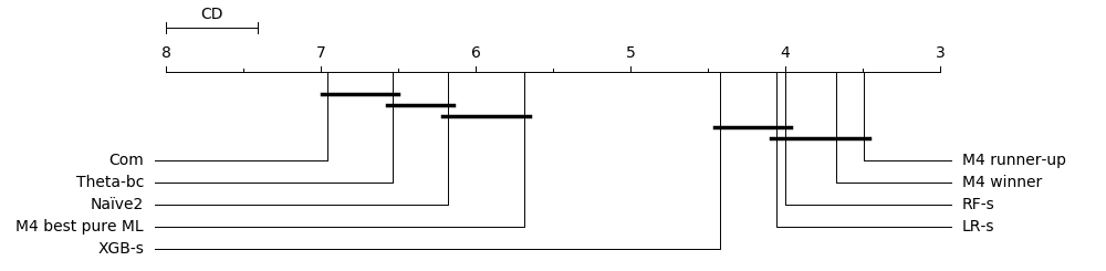
Figure 1: Critical difference diagram based on sMAPE and the hourly data set

Notes: The diagram is based on sMAPE performance and the hourly data set. On the horizontal line, the diagram shows mean ranks for each forecaster. Forecaster grouped by a bar are not statistically significant based on pairwise post-hoc Nemenyi tests at the $5$% level. Corresponding Wilcoxon-Holm test results are shown in the appendix in table 20.

In line with previous results [70, 17], we find that the tried out machine learning models, on average, cannot achieve equal or better performance compared to the statistical models over the whole of the M4 data set.

However, on the hourly data set, machine learning models can perform better than statistical ones. Our best model, RF-s with an OWA of $0.493$ comes even close to the multivariate, hybrid models of the M4 winner ($0.44$) and runner-up ($0.484$). XGB-s ($0.496$) and LR-s ($0.501$) achieve slightly worse, but still competitive performances.

To check if found performance differences are statistically significant, we use significance tests and show a critical difference diagram in figure 1. Corresponding results from Wilcoxon-Holm tests are shown in the appendix in table 20. For the hourly data set, the differences between RF-s and the statistical models are statistically significant, and that the differences between RF-s and the M4 winner and the runner-up are not statistically significant.

To answer question 1: No, standard tabular regression algorithms cannot achieve equal or better performance compared to statistical methods on the whole of the M4 data set. But they can achieve equal or better performance on the hourly data set. Indeed, here they even achieve competitive performance compared to the best performing M4 models, with no significant difference between them.

It is worth emphasising that our tried out models are considerably simpler than the best performing M4 models: they only need a single series for training; they only rely on familiar machine learning techniques; and with sktime, they only require off-the-shelf functionality without any hand-crafted components.

It also appears that the characteristics of the series may be a critical factor determining the performance of machine learning models. This suggests that certain forecasting problem warrant a more systematic exploration of machine learning models, which we hope to further facilitate with sktime.

Table 5: Performance of new machine learning models (OWA)

	Yearly	Quarterly	Monthly	Weekly	Daily	Hourly	Total
M4 winner	0.778	0.847	0.836	0.851	1.046	0.44	0.833
M4 runner-up	0.799	0.847	0.858	0.796	1.019	0.484	0.847
Theta-bc	0.776	0.893	0.904	0.964	0.996	1.009	0.876
Com	0.886	0.885	0.93	0.911	0.982	1.506	0.914
M4 best pure ML	0.859	0.939	0.941	0.996	1.071	0.634	0.926
RF-s	0.967	1.014	0.994	1.015	1.078	0.493	0.994
Naïve2	1.0	1.0	1.0	1.0	1.0	1.0	1.0
XGB-s	1.022	1.091	1.118	1.113	1.149	0.496	1.088
LR-s	-	1.037	2.16	0.964	1.07	0.501	-

• Notes: Rows show forecasters described in table 4. Columns show M4 data sets grouped by sampling frequency. We exclude results for LR model when generated forecasts were instable/exploding due the little available data and linear extrapolation.

Question 2:

Can residual boosting with standard tabular regressors further enhance the predictive performance of Theta-bc, the best statistical model in the M4 study?

To explore the second question, we compare results for Theta-bc with their boosted variants based on the RF and XGB regression algorithms. We also include the tuned versions of the boosted models. Results are shown in table 6. Our key findings are as follows:

On the whole of the M4 data set, boosting does not improve the performance of Theta-bc. While boosting leads to a performance loss on the yearly, monthly and quarterly data sets, it leads to slight performance gains on the weekly, daily and hourly data set. In particular, on the daily data set, boosting with RF improves the OWA of Theta-bc from $0.996$ to $0.988$, and on the hourly data set from $1.009$ to $0.985$. For the weekly data set, tuning is needed to improve accuracy beyond that of Theta-bc.

Again, we test whether found performance differences on the hourly data set are significant. As shown in figure 2, we find that the boosted variants perform significantly better than Theta-bc without boosting, with no significant difference between the boosted variants.

Table 6: Performance of boosted Theta-bc models (OWA)

	Yearly	Quarterly	Monthly	Weekly	Daily	Hourly	Total
Theta-bc	0.776	0.893	0.904	0.964	0.996	1.009	0.876
RF-Theta-bc-t	0.854	0.938	0.933	0.959	0.999	0.987	0.919
RF-Theta-bc	0.864	0.957	0.932	1.052	0.988	0.985	0.925
XGB-Theta-bc	0.898	1.017	0.971	1.153	1.023	0.993	0.968
XGB-Theta-bc-t	0.906	1.009	0.976	1.006	1.04	0.998	0.971

• Notes: Rows show forecasters described in table 4. Columns show M4 data sets grouped by sampling frequency.

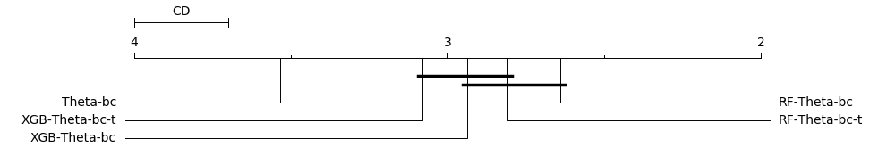
Figure 2: Critical difference diagram based on sMAPE and the hourly data set

Notes: The diagram is based on sMAPE performance and the hourly data set. On the horizontal line, the diagram shows mean ranks for each forecaster. Forecaster grouped by a bar are not statistically significant based on pairwise post-hoc Nemenyi tests at the $5$% level. Corresponding Wilcoxon-Holm test results are shown in the appendix in table 21.

Question 3:

Does tuning the window length hyper-parameter of the reduction from forecasting to tabular regression help improve performance?

To explore the last question, we compare the performance of each regressor, once with a tuned window length and once with the default window length (see table 4). Results are shown in table 7. Our key findings are as follows:

In general, tuning of the window length does not help improve performance. Exceptions are the weekly data set and the KNN regressor. On the weekly data set, all tried out regressors benefit from tuning, with the biggest OWA improvement being $0.082$ for XGB. KNN additionally benefits from tuning on the yearly and hourly data set.

Note that other temporal cross-validation schemes than the one tried out here are possible and may prove to be more beneficial to overall performance (e.g. a sliding window validation). In addition, we may want to try to optimise additional hyper-parameters (e.g. the strategy to generate forecasts as discussed in 3.3.1, or the hyper-parameters of regressor using a nested tabular cross-validation scheme). But note that tuning comes at the cost of a considerable increase in computational running time, as reported in the appendix in table 19.

Table 7: Performance of tuned machine learning models (OWA)

	Yearly	Quarterly	Monthly	Weekly	Daily	Hourly	Total
RF-s	0.967	1.014	0.994	1.015	1.078	0.493	0.994
RF-t-s	1.005	1.070	1.057	0.967	1.087	0.683	1.047
XGB-s	1.022	1.091	1.118	1.113	1.149	0.496	1.088
XGB-t-s	1.038	1.144	1.170	1.031	1.179	0.746	1.131
KNN-s	1.086	1.171	1.257	1.218	1.338	0.544	1.197
KNN-t-s	1.062	1.185	1.276	1.147	1.331	0.751	1.205
LR-s	-	1.037	2.160	0.964	1.070	0.501	-
LR-t-s	-	-	1.876	0.889	1.089	0.670	-

• Notes: Rows show forecasters described in table 4. Columns show M4 data sets grouped by sampling frequency. We exclude LR model results when generated forecasts were instable/exploding, likely due the little available data and linear extrapolation.

6 Conclusion

We presented sktime’s new forecasting framework. sktime integrates with scikit-learn as one of the major machine learning toolboxes, and allows to easily build, tune and evaluate composite machine learning models. We discussed key features of sktime’s forecasting API, including composite models familiar from scikit-learn, but also novel meta-forecasters for reduction and detrending.

In addition, we replicated and extended the M4 forecasting study. Replicating the M4 study allowed us to test our model implementations, and validate published results. We found no or small differences for the naïve and statistical forecasting algorithms, and larger improvements for the machine learning algorithms.

Extending the M4 study allowed us to highlight the usefulness of sktime and to further investigate the potential of simple off-the-shelf machine learning approaches for univariate forecasting. In particular, we found that simple pure approaches like reduction, pipelining and tuning can achieve competitive forecasting performance on the hourly data set, outperforming the statistical algorithms and coming close to the best M4 models. In addition, we found that simple hybrid approaches using residual boosting of statistical methods can help improve their forecasting performance in some cases.

With sktime, we hope to further advance the available toolbox capabilities for time series analysis. In future work, we want to further develop sktime by adding full support for:

• Time series regression algorithms, refactoring existing time series classification algorithm as well as adding bespoke time series regressors,

• Exogenous, multivariate time series, extending bespoke algorithms and adding modular composition techniques specifically for multivariate series,

• Prediction intervals and probabilistic forecasting.

In addition, we hope to develop new frameworks for related learning tasks, including multivariate/panel forecasting and time series annotation (e.g. segmentation and outlier detection).

Authors’ contributions

ML made key contributions to architecture and design, including composition and reduction interfaces. ML is one of sktime’s lead developers, having contributed to almost all parts of it, including the overall toolbox architecture, the time series classification framework, and specific algorithms. ML drafted and wrote most of this manuscript. He wrote the code to replicate and extend the M4 study.

FK conceived the project and architectural outlines, including taxonomy of learning tasks, composition approaches and reduction relations. FK further made key contributions to architecture and design, and contributed to writing of this manuscript.

Appendix

Table 8: The number of M4 series per sampling frequency and domain

	Demographic	Finance	Industry	Macro	Micro	Other	Total
Yearly	1088	6519	3716	3903	6538	1236	23000
Quarterly	1858	5305	4637	5315	6020	865	24000
Monthly	5728	10987	10017	10016	10975	277	48000
Weekly	24	164	6	41	112	12	359
Daily	10	1559	422	127	1476	633	4227
Hourly	0	0	0	0	0	414	414
Total	8708	24534	18798	19402	25121	3437	100000

• Notes: Rows show M4 data sets grouped by sampling frequency. Columns show M4 data sets grouped by domains. Values show the number of available series.

Table 9: Summary statistics of the length of time series in the training set

	Mean	Std	Min	25%	50%	75%	Max
Yearly	31.3	24.5	13	20	29	40	835
Quarterly	92.3	51.1	16	62	88	115	866
Monthly	216.3	137.4	42	82	202	306	2794
Weekly	1022.0	707.1	80	379	934	1603	2597
Daily	2357.4	1756.6	93	323	2940	4197	9919
Hourly	853.9	127.9	700	700	960	960	960
Total	240.0	592.3	13	49	97	234	9919

• Notes: Rows show M4 data sets grouped by sampling frequency. Columns show summary statistics of the distribution of the length of the training series.

Table 10: Replicated M4 forecasters

Name	Category	Description
Naïve	naïve	Always predicting the last observed values.
sNaïve	naïve	Always predicting the last observed value of the same season.
Naïve2	naïve	Like Naïve, but with seasonal adjustment by applying classical multiplicative decomposition [86] and an autocorrelation test at the 90% significance level to decide whether or not to apply seasonal adjustment [87].
SES	statistical	Simple exponential smoothing and extrapolating [88, 89, 90], with no trend, and seasonal adjustment as in Naïve2.
Holt	statistical	Like SES, but with linear trend.
Damped	statistical	Like Holt, but with damped trend [91].
Theta	statistical	As applied to the M3 Competition [67] using two Theta lines, $\theta_{1}=0$ and $\theta_{2}=2$, with the first one being extrapolated using linear regression and the second one using SES. The forecasts are then combined using equal weights [92]. This is equivalent to special case of simple exponential smoothing with drift [93]. Seasonal adjustments are considered as in Naïve2.
Theta-bc	statistical	Like Theta, but with Box-Cox adjustment [94], where lambda is constraint to the $(0,1)$ interval and estimated via maximum likelihood estimation. Submitted to the M4 study by Legaki & Koutsouri (submission number 260).
Com	statistical	Simple arithmetic mean of SES, Holt and Damped.
ARIMA	statistical	An automatic selection of possible seasonal ARIMA models is performed and the best one is chosen using appropriate selection criteria [7, 58].
MLP	ML	A multi-layer perceptron of a very basic architecture and parameterization via a recursive reduction approach as described in section 3.3.1 with window length set to $3$. Linear detrending and seasonal adjustments as in Naïve2 is applied to facilitate extrapolation.
RNN	ML	A recurrent network of a very basic architecture and parameterization via a recursive reduction approach as described in section 3.3.1 with window length set to $3$. Linear detrending and seasonal adjustments as in Naïve2 is applied to facilitate extrapolation.

• Notes: The forecasters are described in detail in the original M4 study [17]. We follow the categorisation of the M4 study here for consistency, but more fruitful categorisations have been proposed by [95].

Table 11: MASE percentage difference between published and replicated results

	Yearly	Quarterly	Monthly	Weekly	Daily	Hourly
Naïve	$0.000$	$0.000$	$0.000$	$0.000$	$0.000$	$0.000$
Naïve2	$0.000$	$0.000$	$0.000$	$0.000$	$0.000$	$-0.000$
sNaïve	$0.000$	$0.000$	$0.000$	$0.000$	$0.000$	$0.000$
SES	$-0.008$	$0.015$	$0.038$	$-0.002$	$0.004$	$0.000$
Holt	$5.586$	$0.001$	$2.805$	$-1.599$	$0.200$	$-3.927$
Damped	$3.696$	$-0.458$	$1.507$	$-2.887$	$0.814$	$-1.154$
Com	$2.751$	$-0.425$	$1.035$	$-1.900$	$0.334$	$-4.332$
ARIMA	$0.141$	$3.329$	$0.991$	$-11.172$	$-4.873$	$4.054$
Theta	$-3.058$	$-1.153$	$-0.139$	$-0.016$	$-0.041$	$0.095$
Theta-bc	$-1.922$	$-1.013$	$-0.202$	$-0.723$	$-0.035$	$-3.606$
MLP	$-14.658$	$-30.207$	$-41.370$	$-80.142$	$-70.993$	$-9.859$
RNN	$-24.522$	$-34.106$	$-30.284$	$-38.831$	$-36.420$	$-20.987$

• Notes: Rows show forecasters described in table 10. Columns show M4 data sets grouped by sampling frequency. Values show the percentage difference between replicated and published MASE values relative to the published values. Negative values indicate that replicated results are lower/better than published ones.

Table 12: OWA percentage difference between replicated and published results

	Yearly	Quarterly	Monthly	Weekly	Daily	Hourly
Naïve	$0.000$	$0.000$	$0.000$	$0.000$	$0.000$	$0.000$
Naïve2	$0.000$	$0.000$	$0.000$	$0.000$	$0.000$	$0.000$
sNaïve	$0.000$	$-0.000$	$0.000$	$0.000$	$0.000$	$0.000$
SES	$-0.006$	$0.042$	$0.027$	$-0.003$	$0.007$	$0.000$
Holt	$4.782$	$-0.812$	$3.382$	$-2.568$	$0.244$	$-4.048$
Damped	$2.594$	$-0.753$	$0.751$	$-1.729$	$0.926$	$-0.984$
Com	$2.179$	$-0.524$	$1.080$	$-1.646$	$0.416$	$-3.256$
ARIMA	$0.909$	$3.984$	$1.727$	$-5.082$	$-3.502$	$0.053$
Theta	$-2.267$	$-0.541$	$-0.031$	$0.081$	$0.008$	$0.053$
Theta-bc	$-1.416$	$-0.542$	$-0.147$	$-0.372$	$0.008$	$-0.308$
MLP	$-13.251$	$-27.165$	$-34.713$	$-71.246$	$-66.951$	$-7.691$
RNN	$-23.582$	$-31.657$	$-30.563$	$-32.746$	$-34.685$	$-16.490$

• Notes: Rows show forecasters described in table 10. Columns show M4 data sets grouped by sampling frequency. Values show the percentage difference between replicated and published OWA values relative to the published values. Negative values indicate that replicated results are lower/better than published ones.

Table 13: sMAPE difference between published and replicated results

	Yearly	Quarterly	Monthly	Weekly	Daily	Hourly
Naïve	$-0.0$ p m 0.0	$0.0$ p m 0.0	$0.0$ p m 0.0	$0.0$ p m 0.0	$0.0$ p m 0.0	$0.0$ p m 0.0
Naïve2	$-0.0$ p m 0.0	$-0.0$ p m 0.0	$0.0$ p m 0.0	$0.0$ p m 0.0	$0.0$ p m 0.0	$0.0$ p m 0.0
sNaïve	$-0.0$ p m 0.0	$0.0$ p m 0.0	$0.0$ p m 0.0	$0.0$ p m 0.0	$0.0$ p m 0.0	$0.0$ p m 0.0
SES	$-0.001$ p m 0.006	$0.007$ p m 0.004	$0.002$ p m 0.001	$-0.0$ p m 0.0	$0.0$ p m 0.0	$0.0$ p m 0.0
Holt	$0.665$ p m 0.083	$-0.167$ p m 0.034	$0.58$ p m 0.044	$-0.327$ p m 0.107	$0.009$ p m 0.013	$-1.271$ p m 0.463
Damped	$0.241$ p m 0.056	$-0.105$ p m 0.023	$0.001$ p m 0.02	$-0.062$ p m 0.042	$0.032$ p m 0.021	$-0.151$ p m 0.151
Com	$0.246$ p m 0.042	$-0.063$ p m 0.016	$0.151$ p m 0.016	$-0.127$ p m 0.037	$0.015$ p m 0.007	$-0.339$ p m 0.171
ARIMA	$0.245$ p m 0.058	$0.477$ p m 0.038	$0.325$ p m 0.035	$0.074$ p m 0.285	$-0.068$ p m 0.023	$-0.282$ p m 0.389
Theta	$-0.221$ p m 0.017	$0.005$ p m 0.007	$0.01$ p m 0.004	$0.016$ p m 0.006	$0.002$ p m 0.002	$0.001$ p m 0.0
Theta-bc	$-0.127$ p m 0.017	$-0.01$ p m 0.005	$-0.012$ p m 0.004	$-0.004$ p m 0.006	$0.002$ p m 0.001	$0.593$ p m 0.242
MLP	$-2.598$ p m 0.048	$-4.46$ p m 0.062	$-6.708$ p m 0.062	$-11.229$ p m 1.046	$-5.754$ p m 0.179	$-0.631$ p m 0.127
RNN	$-5.091$ p m 0.091	$-4.994$ p m 0.073	$-7.413$ p m 0.089	$-3.954$ p m 0.785	$-1.968$ p m 0.113	$-1.372$ p m 0.383

• Notes: Rows show forecasters described in table 10. Columns show M4 data sets grouped by sampling frequency. Values show the difference between replicated and published mean sMAPE values, together with the standard error of the difference in means between paired samples. Values in bold indicate that the difference is statistically significant at the $95\%$ level based on a two-sided paired t-test. Negative values indicate that replicated results are lower than published ones.

Table 14: MASE difference between published and replicated results

	Yearly	Quarterly	Monthly	Weekly	Daily	Hourly
Naïve	$0.0$ p m 0.0	$0.0$ p m 0.0	$0.0$ p m 0.0	$0.0$ p m 0.0	$0.0$ p m 0.0	$0.0$ p m 0.0
Naïve2	$0.0$ p m 0.0	$0.0$ p m 0.0	$0.0$ p m 0.0	$0.0$ p m 0.0	$0.0$ p m 0.0	$0.0$ p m 0.0
sNaïve	$0.0$ p m 0.0	$0.0$ p m 0.0	$0.0$ p m 0.0	$0.0$ p m 0.0	$0.0$ p m 0.0	$0.0$ p m 0.0
SES	$-0.0$ p m 0.0	$0.0$ p m 0.0	$0.0$ p m 0.0	$-0.0$ p m 0.0	$0.0$ p m 0.0	$0.0$ p m 0.0
Holt	$0.198$ p m 0.012	$0.0$ p m 0.002	$0.028$ p m 0.002	$-0.039$ p m 0.012	$0.006$ p m 0.009	$-0.367$ p m 0.168
Damped	$0.125$ p m 0.008	$-0.005$ p m 0.002	$0.015$ p m 0.005	$-0.069$ p m 0.023	$0.026$ p m 0.024	$-0.034$ p m 0.116
Com	$0.09$ p m 0.006	$-0.005$ p m 0.001	$0.01$ p m 0.002	$-0.046$ p m 0.012	$0.011$ p m 0.007	$-0.199$ p m 0.062
ARIMA	$0.005$ p m 0.01	$0.039$ p m 0.003	$0.009$ p m 0.002	$-0.286$ p m 0.115	$-0.166$ p m 0.024	$0.038$ p m 0.024
Theta	$-0.103$ p m 0.002	$-0.014$ p m 0.0	$-0.001$ p m 0.0	$-0.0$ p m 0.003	$-0.001$ p m 0.001	$0.002$ p m 0.0
Theta-bc	$-0.058$ p m 0.005	$-0.012$ p m 0.001	$-0.002$ p m 0.0	$-0.019$ p m 0.008	$-0.001$ p m 0.001	$-0.092$ p m 0.05
MLP	$-0.725$ p m 0.027	$-0.699$ p m 0.019	$-0.796$ p m 0.045	$-10.874$ p m 5.053	$-9.21$ p m 1.916	$-0.257$ p m 0.033
RNN	$-1.213$ p m 0.028	$-0.688$ p m 0.008	$-0.485$ p m 0.005	$-1.993$ p m 0.263	$-2.27$ p m 0.114	$-0.64$ p m 0.248

• Notes: Rows show forecasters described in table 10. Columns show M4 data sets grouped by sampling frequency. Values show the difference between replicated and published mean MASE values, together with the standard error of the difference in means between paired samples. Values in bold indicate that the difference is statistically significant at the $95\%$ level based on a two-sided paired t-test. Negative values indicate that replicated results are lower than published ones.

Table 15: Tabular regression algorithms used to extend the M4 study

Name	Description	Hyper-parameters
LR	Linear regression	fit_intercept=True
KNN	K-nearest neighbours	n_neighbors=1
RF	Random forest	n_estimators=500
XGB	Gradient boosted trees	n_estimators=500

• Notes: For all algorithms except XGB, we use scikit-learn. For XGB, we use xgboost [83]. For all other hyper-parameters, we use the packages’ default settings.

Table 16: Complete results (sMAPE)

	Yearly	Quarterly	Monthly	Weekly	Daily	Hourly
Theta-bc	13.239	10.145	12.99	9.144	3.042	18.16
Theta	14.372	10.316	13.012	9.109	3.055	18.14
Com	15.094	10.112	13.585	8.817	2.995	21.714
RF-Theta-bc-t	14.552	10.788	13.543	9.014	3.056	18.136
Damped	15.439	10.132	13.475	8.804	3.096	19.114
RF-Theta-bc	14.738	11.006	13.527	9.801	3.061	18.061
ARIMA	15.413	10.908	13.768	8.727	3.124	13.698
SES	16.395	10.607	13.62	9.011	3.045	18.094
XGB-Theta-bc-t	15.334	11.535	14.166	9.484	3.134	18.303
XGB-Theta-bc	15.395	11.651	14.109	10.808	3.16	18.199
Naïve2	16.342	11.012	14.427	9.161	3.045	18.383
KNN-Theta-bc	15.503	12.046	14.805	11.133	3.189	19.32
KNN-Theta-bc-t	15.507	12.036	14.877	10.17	3.189	19.361
RF-s	16.655	11.674	14.899	9.327	3.291	10.978
RF	16.656	11.793	15.01	9.31	3.289	13.663
Holt	17.018	10.74	15.393	9.381	3.075	27.978
Naïve	16.342	11.61	15.256	9.161	3.045	43.003
sNaïve	16.342	12.521	15.988	9.161	3.045	13.912
RF-t-s	17.31	12.321	16.008	9.009	3.321	15.797
RNN	17.307	12.033	16.643	11.266	3.996	13.326
XGB-s	17.729	12.633	17.158	10.201	3.512	10.912
XGB	17.729	12.671	17.259	10.201	3.512	14.288
LR-s	-	12.235	17.768	9.519	3.32	11.235
LR	-	12.238	17.797	9.519	3.32	16.342
XGB-t-s	17.954	13.21	18.102	9.462	3.608	17.195
MLP	19.166	14.04	17.625	10.12	3.568	13.211
KNN-t-s	18.37	13.701	19.711	10.482	4.062	16.333
KNN-s	18.758	13.548	19.764	11.167	4.08	11.988
KNN	18.758	13.606	19.905	11.167	4.08	14.61
LR-t-s	-	-	18.619	8.567	3.363	16.76

• Notes: Rows show forecasters described in table 4. Columns show M4 data sets grouped by sampling frequency. We exclude LR model results when generated forecasts were instable/exploding, likely due the little available data and linear extrapolation.

Table 17: Complete results (MASE)

	Yearly	Quarterly	Monthly	Weekly	Daily	Hourly
Theta-bc	2.951	1.186	0.964	2.582	3.252	2.465
Theta	3.279	1.218	0.968	2.637	3.261	2.457
RF-Theta-bc-t	3.246	1.229	0.985	2.592	3.257	2.363
ARIMA	3.407	1.204	0.939	2.27	3.244	0.981
RF-Theta-bc	3.282	1.253	0.984	2.87	3.18	2.365
Com	3.371	1.168	0.976	2.386	3.213	4.383
Damped	3.504	1.168	0.987	2.334	3.262	2.922
XGB-Theta-bc	3.392	1.338	1.025	3.127	3.309	2.387
XGB-Theta-bc-t	3.476	1.332	1.032	2.713	3.446	2.398
KNN-Theta-bc	3.394	1.366	1.069	3.01	3.365	2.52
KNN-Theta-bc-t	3.396	1.368	1.083	2.842	3.4	2.529
RF-s	3.639	1.327	1.016	2.809	3.523	0.93
RF	3.64	1.341	1.037	2.823	3.521	1.032
Holt	3.748	1.198	1.038	2.381	3.23	8.988
RF-t-s	3.779	1.399	1.068	2.639	3.553	1.212
SES	3.98	1.34	1.02	2.684	3.281	2.385
RNN	3.733	1.329	1.116	3.139	3.962	2.408
Naïve2	3.974	1.371	1.063	2.777	3.278	2.395
XGB-s	3.814	1.42	1.113	3.091	3.754	0.954
XGB	3.814	1.431	1.129	3.091	3.754	1.063
XGB-t-s	3.883	1.493	1.154	2.857	3.847	1.335
Naïve	3.974	1.477	1.205	2.777	3.278	11.608
sNaïve	3.974	1.602	1.26	2.777	3.278	1.193
MLP	4.221	1.615	1.129	2.694	3.763	2.35
KNN-s	4.072	1.524	1.217	3.378	4.38	1.044
KNN-t-s	3.977	1.543	1.261	3.192	4.355	1.471
KNN	4.072	1.534	1.239	3.378	4.38	1.112
LR-s	-	1.319	3.284	2.467	3.442	0.934
LR	-	1.327	3.301	2.467	3.442	1.001
LR-t-s	-	-	2.618	2.338	3.518	1.027

• Notes: Rows show forecasters described in table 4. Columns show M4 data sets grouped by sampling frequency. We exclude LR model results when generated forecasts were instable/exploding, likely due the little available data and linear extrapolation.

Table 18: OWA

	Yearly	Quarterly	Monthly	Weekly	Daily	Hourly
Theta-bc	0.776	0.893	0.904	0.964	0.996	1.009
Theta	0.852	0.912	0.906	0.972	0.999	1.006
Com	0.886	0.885	0.93	0.911	0.982	1.506
RF-Theta-bc-t	0.854	0.938	0.933	0.959	0.999	0.987
ARIMA	0.9	0.934	0.919	0.885	1.008	0.577
Damped	0.913	0.886	0.931	0.901	1.006	1.13
RF-Theta-bc	0.864	0.957	0.932	1.052	0.988	0.985
XGB-Theta-bc	0.898	1.017	0.971	1.153	1.023	0.993
SES	1.002	0.97	0.952	0.975	1.0	0.99
XGB-Theta-bc-t	0.906	1.009	0.976	1.006	1.04	0.998
RF-s	0.967	1.014	0.994	1.015	1.078	0.493
Holt	0.992	0.924	1.021	0.941	0.997	2.637
KNN-Theta-bc	0.901	1.045	1.016	1.149	1.037	1.052
Naïve2	1.0	1.0	1.0	1.0	1.0	1.0
KNN-Theta-bc-t	0.902	1.045	1.025	1.067	1.042	1.055
RF	0.967	1.025	1.008	1.016	1.077	0.587
RF-t-s	1.005	1.07	1.057	0.967	1.087	0.683
RNN	0.999	1.031	1.102	1.18	1.26	0.865
Naïve	1.0	1.066	1.095	1.0	1.0	3.593
XGB-s	1.022	1.091	1.118	1.113	1.149	0.496
XGB	1.022	1.097	1.129	1.113	1.149	0.611
sNaïve	1.0	1.153	1.146	1.0	1.0	0.628
XGB-t-s	1.038	1.144	1.17	1.031	1.179	0.746
MLP	1.117	1.226	1.142	1.037	1.16	0.85
KNN-s	1.086	1.171	1.257	1.218	1.338	0.544
KNN-t-s	1.062	1.185	1.276	1.147	1.331	0.751
KNN	1.086	1.177	1.272	1.218	1.338	0.63
LR-s	-	1.037	2.16	0.964	1.07	0.501
LR	-	1.039	2.169	0.964	1.07	0.654
LR-t-s	-	-	1.876	0.889	1.089	0.67

• Notes: Rows show forecasters described in table 4. Columns show M4 data sets grouped by sampling frequency. We exclude LR model results when generated forecasts were instable/exploding, likely due the little available data and linear extrapolation.

Table 19: Summary results of new machine learning models

	sMAPE	MASE	OWA	Running time (min)
Theta-bc	11.952	1.583	0.876	8.1
Theta	12.264	1.669	0.9	6.27
Com	12.668	1.687	0.914	69.47
RF-Theta-bc-t	12.673	1.671	0.919	14539.77
ARIMA	12.992	1.673	0.92	14992.88
Damped	12.692	1.718	0.92	53.45
RF-Theta-bc	12.763	1.682	0.925	1189.37
XGB-Theta-bc	13.357	1.754	0.968	122.94
SES	13.09	1.885	0.97	5.9
XGB-Theta-bc-t	13.337	1.78	0.971	1826.44
RF-s	14.002	1.806	0.994	1168.56
Holt	14.16	1.83	0.997	11.72
KNN-Theta-bc	13.818	1.785	0.998	64.36
Naïve2	13.564	1.912	1.0	3.66
KNN-Theta-bc-t	13.848	1.794	1.003	656.04
RF	14.095	1.82	1.004	1163.64
RF-t-s	14.86	1.882	1.047	14165.87
RNN	15.122	1.902	1.067	38941.68
Naïve	14.208	2.044	1.072	1.04
XGB-s	15.576	1.926	1.088	116.95
XGB	15.647	1.937	1.096	115.76
sNaïve	14.657	2.057	1.105	1.03
XGB-t-s	16.246	1.983	1.131	1718.15
MLP	16.48	2.079	1.156	157.88
KNN-s	17.315	2.088	1.197	58.71
KNN-t-s	17.252	2.092	1.205	634.12
KNN	17.407	2.101	1.207	56.99
LR-s	-	-	-	55.36
LR	-	-	-	53.37
LR-t-s	-	-	-	590.87

• Notes: Rows show forecasters described in table 4. Columns show aggregate values for sMAPE, MASE and OWA metrics, as well as the total running time in minutes scaled to the number of CPUs used in the original M4 study, as described in section 5. We exclude LR model results when generated forecasts were instable/exploding, likely due the little available data and linear extrapolation.

Table 20: Post-hoc Wilcoxon signed rank tests results for pairwise comparisons on the hourly data set

	forecaster A	forecaster B	p-value
0	LR-s	RF-s	0.657
4	LR-s	XGB-s	0.243
3	M4 runner-up	M4 winner	0.317
2	M4 runner-up	RF-s	0.468
1	RF-s	XGB-s	0.010

• Notes: This table corresponds to the results presented in figure 1. The results are based on sMAPE and the hourly data set. We only show pairs of forecasters which are not significantly different. Forecasters are described in table 4. We use Wilcoxon signed rank tests to compute p-values. Significance at the $5$% is established using Holm’s procedure for correcting for multiple testing, as discussed in 5.2.

Table 21: Post-hoc Wilcoxon signed rank tests results for pairwise comparisons on the hourly data set

	forecaster A	forecaster B	p-value
2	RF-Theta-bc	RF-Theta-bc-t	0.096
1	RF-Theta-bc-t	XGB-Theta-bc	0.092
3	Theta-bc	XGB-Theta-bc-t	0.527
0	XGB-Theta-bc	XGB-Theta-bc-t	0.028

• Notes: This table corresponds to the results presented in figure 2. The results are based on sMAPE and the hourly data set. We only show pairs of forecasters which are not significantly different. Forecasters are described in table 4. We use Wilcoxon signed rank tests to compute p-values. Significance at the $5$% is established using Holm’s procedure for correcting for multiple testing, as discussed in 5.2.

References

- Smyl [2020] Slawek Smyl. A hybrid method of exponential smoothing and recurrent neural networks for time series forecasting. International Journal of Forecasting, 36(1):75–85, 2020.
- Oreshkin et al. [2019] Boris N Oreshkin, Dmitri Carpov, Nicolas Chapados, and Yoshua Bengio. N-BEATS: Neural basis expansion analysis for interpretable time series forecasting. arXiv preprint arXiv:1905.10437, 2019.
- Buitinck et al. [2013] Lars Buitinck, Gilles Louppe, Mathieu Blondel, Fabian Pedregosa, Andreas C Müller, Olivier Grisel, Vlad Niculae, Peter Prettenhofer, Alexandre Gramfort, Jaques Grobler, Robert Layton, Jake Vanderplas, Arnaud Joly, Brian Holt, and Gaël Varoquaux. API design for machine learning software: experiences from the scikit-learn project. ArXiv e-prints, 2013. URL https://github.com/scikit-learn.
- Löning et al. [2019] Markus Löning, Anthony Bagnall, Sajaysurya Ganesh, Viktor Kazakov, Jason Lines, and Franz J Király. sktime: A Unified Interface for Machine Learning with Time Series. In Workshop on Systems for ML at NeurIPS 2019, 2019.
- M4 Team and others [2018a] M4 Team and others. M4 competitor’s guide: Prizes and rules, 2018a. URL https://www.m4.unic.ac.cy/wp-content/uploads/2018/03/M4-Competitors-Guide.pdf.
- Makridakis et al. [2018a] Spyros Makridakis, Evangelos Spiliotis, and Vassilios Assimakopoulos. The M4 Competition: Results, findings, conclusion and way forward. International Journal of Forecasting, 34(4):802–808, 2018a. ISSN 01692070. doi: 10.1016/j.ijforecast.2018.06.001.
- Box et al. [2015] George E. P. Box, Gwilym M. Jenkins, Gregory C. Reinsel, and Greta M. Ljung. Time series analysis: forecasting and control. John Wiley & Sons, 2015. ISBN 9781118674925.
- Brockwell and Davis [2016] Peter J. Brockwell and Richard A. Davis. Introduction to Time Series and Forecasting. Springer Texts in Statistics. Springer International Publishing, 2016. ISBN 978-3-319-29852-8. doi: 10.1007/978-3-319-29854-2. URL http://link.springer.com/10.1007/978-3-319-29854-2.
- Hyndman et al. [2018] Rob J Hyndman, George Athanasopoulos, Christoph Bergmeir, Gabriel Caceres, Leanne Chhay, Mitchell O’Hara-Wild, Fotios Petropoulos, Slava Razbash, Earo Wang, and Farah Yasmeen. forecast: Forecasting functions for time series and linear models, 4 2018. URL https://researchportal.bath.ac.uk/en/publications/forecast-forecasting-functions-for-time-series-and-linear-models.
- De Gooijer and Hyndman [2006] Jan G De Gooijer and Rob J Hyndman. 25 years of time series forecasting. International journal of forecasting, 22(3):443–473, 2006.
- Erich et al. [1997] Gamma Erich, Richard Helm, Ralph Johnson, and John Vlissides. Design Patterns – Elements of Reusable Object-Oriented Software. Addison Wesley Longman, Inc., 1997. ISBN 9780201715941. doi: 10.1093/carcin/bgs084.
- Makridakis et al. [2018b] Spyros Makridakis, Vassilios Assimakopoulos, and Evangelos Spiliotis. Objectivity, reproducibility and replicability in forecasting research, 2018b. ISSN 01692070.
- Boylan et al. [2015] John E. Boylan, Paul Goodwin, Maryam Mohammadipour, and Aris A. Syntetos. Reproducibility in forecasting research. International Journal of Forecasting, 2015. ISSN 01692070. doi: 10.1016/j.ijforecast.2014.05.008.
- Hyndman [2010] Rob J. Hyndman. Encouraging replication and reproducible research, 2010. ISSN 01692070.
- Arnold et al. [2019] Becky Arnold, Louise Bowler, Sarah Gibson, Patricia Herterich, Rosie Higman, Anna Krystalli, Alexander Morley, Martin O’Reilly, Kirstie Whitaker, and Others. The Turing Way: A Handbook for Reproducible Data Science. 3 2019. doi: 10.5281/ZENODO.3233986. URL 10.5281/zenodo.3233853.
- Bergmeir et al. [2018] Christoph Bergmeir, Rob J Hyndman, and Bonsoo Koo. A note on the validity of cross-validation for evaluating autoregressive time series prediction. Computational Statistics & Data Analysis, 120:70–83, 2018.
- Makridakis et al. [2019] Spyros Makridakis, Evangelos Spiliotis, and Vassilios Assimakopoulos. The M4 Competition: 100,000 time series and 61 forecasting methods. International Journal of Forecasting, 2019.
- Montero-Manso et al. [2020] Pablo Montero-Manso, George Athanasopoulos, Rob J Hyndman, and Thiyanga S Talagala. FFORMA: Feature-based forecast model averaging. International Journal of Forecasting, 36(1):86–92, 2020.
- Perktold and Seabold [2010] Josef Perktold and Skipper Seabold. Statsmodels: Econometric and Statistical Modeling with Python Quantitative histology of aorta View project Statsmodels: Econometric and Statistical Modeling with Python. In Proceedings of the 9th Python in Science Conference, 2010. URL https://www.researchgate.net/publication/264891066.
- Bontempi et al. [2013] Gianluca Bontempi, Souhaib Ben Taieb, and Yann-Aël Le Borgne. Machine Learning Strategies for Time Series Forecasting. In Business Intelligence, pages 62–77. Springer, Berlin, Heidelberg, 2013.
- Beygelzimer et al. [2005] Alina Beygelzimer, John Langford, and Bianca Zadrozny. Weighted one-against-all. In American Association for Artificial Intelligence (AAAI), pages 720–725, 2005.
- Beygelzimer et al. [2008] Alina Beygelzimer, John Langford, and Bianca Zadrozny. Machine learning techniques—reductions between prediction quality metrics. In Performance Modeling and Engineering, pages 3–28. Springer, 2008.
- Taieb [2014] Souhaib Ben Taieb. Machine learning strategies for multi-step-ahead time series forecasting. PhD thesis, Universit Libre de Bruxelles, Belgium, 2014.
- Taieb and Hyndman [2014] Souhaib Ben Taieb and Rob J. Hyndman. Boosting multi-step autoregressive forecasts. In 31st International Conference on Machine Learning, ICML 2014, 2014. ISBN 9781634393973.
- Chan and Pauwels [2018] Felix Chan and Laurent L. Pauwels. Some theoretical results on forecast combinations. International Journal of Forecasting, 2018. ISSN 01692070. doi: 10.1016/j.ijforecast.2017.08.005.
- Smith and Wallis [2009] Jeremy Smith and Kenneth F Wallis. A simple explanation of the forecast combination puzzle. Oxford Bulletin of Economics and Statistics, 71(3):331–355, 2009.
- Timmermann [2006] Allan Timmermann. Forecast combinations. In Handbook of economic forecasting, volume 1, chapter 4, pages 135–196. Elsevier, 2006.
- Clemen [1989] Robert T Clemen. Combining forecasts: A review and annotated bibliography. International Journal of Forecasting, 5(4):559–583, 1989.
- Bates and Granger [1969] John M Bates and Clive W J Granger. The combination of forecasts. Journal of the Operational Research Society, 20(4):451–468, 1969.
- Bagnall et al. [2017] Anthony Bagnall, Jason Lines, Aaron Bostrom, James Large, and Eamonn Keogh. The great time series classification bake off: a review and experimental evaluation of recent algorithmic advances. Data Mining and Knowledge Discovery, 31(3):606–660, 5 2017. ISSN 1384-5810. doi: 10.1007/s10618-016-0483-9. URL http://link.springer.com/10.1007/s10618-016-0483-9.
- Christ et al. [2016] Maximilian Christ, Andreas W. Kempa-Liehr, and Michael Feindt. Distributed and parallel time series feature extraction for industrial big data applications. ArXiv e-prints, 10 2016. URL http://arxiv.org/abs/1610.07717.
- Christ et al. [2018] Maximilian Christ, Nils Braun, Julius Neuffer, and Andreas W. Kempa-Liehr. Time Series FeatuRe Extraction on basis of Scalable Hypothesis tests (tsfresh – A Python package). Neurocomputing, 307:72–77, 9 2018. ISSN 0925-2312. doi: 10.1016/J.NEUCOM.2018.03.067. URL https://www.sciencedirect.com/science/article/pii/S0925231218304843?via%3Dihub.
- van der Walt et al. [2011] Stéfan van der Walt, S Chris Colbert, and Gaël Varoquaux. The NumPy Array: A Structure for Efficient Numerical Computation. Computing in Science & Engineering, 13(2):22–30, 3 2011. ISSN 1521-9615. doi: 10.1109/MCSE.2011.37. URL http://ieeexplore.ieee.org/document/5725236/.
- Oliphant [2015] Travis E. Oliphant. Guide to NumPy. CreateSpace Independent Publishing Platform, 2nd edition, 2015. ISBN 151730007X.
- McKinney [2011] Wes McKinney. pandas: a Foundational Python Library for Data Analysis and Statistics. In Python for High Performance and Scientific Computing, 2011.
- Jones et al. [2001] Eric Jones, Travis E. Oliphant, Pearu Peterson, and others. SciPy: Open source scientific tools for Python, 2001. URL http://www.scipy.org/.
- Haenel et al. [2013] V. Haenel, E. Gouillart, and Gaël Varoquaux. Python scientific lecture notes, 2013. URL http://scipy-lectures.github.io/.
- Varoquaux et al. [2015] Gaël Varoquaux, L. Buitinck, Gilles Louppe, Olivier Grisel, F. Pedregosa, and A. Mueller. Scikit-learn: Machine Learning Without Learning the Machinery. GetMobile: Mobile Computing and Communications, 19(1):29–33, 6 2015. doi: 10.1145/2786984.2786995. URL http://dl.acm.org/citation.cfm?doid=2786984.2786995.
- Pedregosa et al. [2011] Fabian Pedregosa, Gaël Varoquaux, Alexandre Gramfort, Vincent Michel, Bertrand Thirion, Olivier Grisel, Mathieu Blondel, Peter Prettenhofer, Ron Weiss, Vincent Dubourg, Jake Vanderplas, Alexandre Passos, David Cournapeau, Matthieu Brucher, Matthieu Perrot, and Édouard Duchesnay. Scikit-learn: Machine Learning in Python. The Journal of Machine Learning Research, 12:2825–2830, 2011. URL https://dl.acm.org/citation.cfm?id=2078195.
- Lam et al. [2015] Siu Kwan Lam, Antoine Pitrou, and Stanley Seibert. Numba: A LLVM-based python JIT compiler. Proceedings of the Second Workshop on the LLVM Compiler Infrastructure in HPC - LLVM ’15, 2015. doi: 10.1145/2833157.2833162.
- Behnel et al. [2011] Stefan Behnel, Robert Bradshaw, Craig Citro, Lisandro Dalcin, Dag Sverre Seljebotn, and Kurt Smith. Cython: The best of both worlds. Computing in Science & Engineering, 13(2):31–39, 2011.
- Abadi et al. [2016] Martin Abadi, Paul Barham, Jianmin Chen, Zhifeng Chen, Andy Davis, Jeffrey Dean, Matthieu Devin, Sanjay Ghemawat, Geoffrey Irving, Michael Isard, and others. TensorFlow: A system for large-scale machine learning. In 12th USENIX Symposium on Operating Systems Design and Implementation (OSDI 16), pages 265–283, 2016.
- Chollet and others [2015] François Chollet and others. Keras. https://keras.io, 2015.
- Bussonnier et al. [2018] Matthias Bussonnier, Jessica Forde, Jeremy Freeman, Brian Granger, Tim Head, Chris Holdgraf, Kyle Kelley, Gladys Nalvarte, Andrew Osheroff, M Pacer, Yuvi Panda, Fernando Perez, Benjamin Ragan-Kelley, and Carol Willing. Binder 2.0 - Reproducible, interactive, sharable environments for science at scale. In Fatih Akici, David Lippa, Dillon Niederhut, and M Pacer, editors, Proceedings of the 17th Python in Science Conference, pages 113–120, 2018. doi: 10.25080/Majora-4af1f417-011.
- Holmes et al. [1994] G. Holmes, A. Donkin, and I.H. Witten. WEKA: a machine learning workbench. In Proceedings of ANZIIS ’94 - Australian New Zealnd Intelligent Information Systems Conference, pages 357–361. IEEE, 1994. ISBN 0-7803-2404-8. doi: 10.1109/ANZIIS.1994.396988. URL http://ieeexplore.ieee.org/document/396988/.
- Hall et al. [2009] Mark Hall, Eibe Frank, Geoffrey Holmes, Bernhard Pfahringer, Peter Reutemann, and Ian H. Witten. The WEKA data mining software. ACM SIGKDD Explorations Newsletter, 11(1):10, 11 2009. ISSN 19310145. doi: 10.1145/1656274.1656278. URL http://portal.acm.org/citation.cfm?doid=1656274.1656278.
- Blaom et al. [2020] Anthony Blaom, Thibaut Lienart, Yiannis Simillides, Diego Arenas, vollmersj, Mosè Giordano, Okon Samuel, Ayush Shridhar, Ayush Shridhar, Ed, swenkel, Julian Samaroo, evalparse, Júlio Hoffimann, sjvollmer, Michael Krabbe Borregaard, Kevin Squire, pshashk, lhnguyen-vn, azev77, Ashrya Agrawal, Venkateshprasad, Robert Hönig, Nils, Kryohi, Julia TagBot, Evelina Gabasova, Dilum Aluthge, and Cédric St-Jean. MLJ: A Machine Learning Framework for Julia, 4 2020. URL https://zenodo.org/record/3765808.
- Bischl et al. [2016] Bernd Bischl, Michel Lang, Lars Kotthoff, Julia Schiffner, Jakob Richter, Erich Studerus, Giuseppe Casalicchio, and Zachary M. Jones. mlr: Machine Learning in R. Journal of Machine Learning Research, 17(170):1–5, 2016. URL http://jmlr.org/papers/v17/15-066.html.
- Kuhn [2008] Max Kuhn. Building Predictive Models in R: Using the caret Package. Journal of Statistical Software, 28(5), 2008. doi: 10.18637/jss.v028.i05. URL http://www.jstatsoft.org/v28/i05/.
- Kuhn et al. [2018] Max Kuhn, Jed Wing, Steve Weston, Andre Williams, Chris Keefer, Allan Engelhardt, Tony Cooper, Zachary Mayer, Brenton Kenkel, Michael Benesty, Reynald Lescarbeau, Andrew Ziem, Luca Scrucca, Yuan Tang, Can Candan, and Tyler Hunt. caret: Classification and Regression Training, 2018. URL https://cran.r-project.org/web/packages/caret/index.html.
- Faouzi and Janati [2020] Johann Faouzi and Hicham Janati. pyts: A Python Package for Time Series Classification. Journal of Machine Learning Research, 21(46):1–6, 2020.
- Burns et al. [2018] David M Burns, Cari M Whyne, David M Burns, and Cari M Whyne. Seglearn: a python package for learning sequences and time series. The Journal of Machine Learning Research, 19(1):3238–3244, 2018.
- Kanter and Veeramachaneni [2015] James Max Kanter and Kalyan Veeramachaneni. Deep feature synthesis: Towards automating data science endeavors. In 2015 IEEE International Conference on Data Science and Advanced Analytics, DSAA 2015, Paris, France, October 19-21, 2015, pages 1–10. IEEE, 2015.
- Lubba et al. [2019] Carl H Lubba, Sarab S Sethi, Philip Knaute, Simon R Schultz, Ben D Fulcher, and Nick S Jones. catch22: CAnonical Time-series CHaracteristics. Data Mining and Knowledge Discovery, 33(6):1821–1852, 2019.
- Fulcher and Jones [2017] Ben D Fulcher and Nick S Jones. hctsa: A Computational Framework for Automated Time-Series Phenotyping Using Massive Feature Extraction. Cell systems, 5(5):527–531, 11 2017. ISSN 2405-4712. doi: 10.1016/j.cels.2017.10.001. URL http://www.ncbi.nlm.nih.gov/pubmed/29102608.
- Fulcher and Jones [2014] Ben D Fulcher and Nick S Jones. Highly Comparative Feature-Based Time-Series Classification. IEEE Transactions on Knowledge and Data Engineering, 26(12):3026–3037, 12 2014. ISSN 1041-4347. doi: 10.1109/TKDE.2014.2316504. URL http://ieeexplore.ieee.org/document/6786425/.
- Hamilton [2017] Mark Hamilton. tseries: a library for time series analysis with sklearn, 9 2017. URL https://zenodo.org/record/897193.
- Hyndman and Khandakar [2008] Rob J Hyndman and Yeasmin Khandakar. Automatic time series forecasting: the forecast package for {R}. Journal of Statistical Software, 26(3):1–22, 2008. URL http://www.jstatsoft.org/article/view/v027i03.
- Alexandrov et al. [2019] Alexander Alexandrov, Konstantinos Benidis, Michael Bohlke-Schneider, Valentin Flunkert, Jan Gasthaus, Tim Januschowski, Danielle C Maddix, Syama Rangapuram, David Salinas, Jasper Schulz, and others. Gluonts: Probabilistic time series models in python. arXiv preprint arXiv:1906.05264, 2019.
- Smith and Others [2019] Taylor G. Smith and Others. pmdarima: ARIMA estimators for Python, 2019. URL http://www.alkaline-ml.com/pmdarima.
- Taylor [2016] Ross Taylor. PyFlux: An open source time series library for Python, 2016. URL http://www.pyflux.com.
- Taylor and Letham [2018] Sean J Taylor and Benjamin Letham. Forecasting at scale. The American Statistician, 72(1):37–45, 9 2018. doi: 10.7287/peerj.preprints.3190v2. URL https://peerj.com/preprints/3190/.
- Snow [2020] Derek Snow. AtsPy: Automated Time Series Models in Python, 2020. URL https://github.com/firmai/atspy/.
- Makridakis et al. [1982] Spyros Makridakis, A Andersen, Robert Carbone, Robert Fildes, Michele Hibon, Rudolf Lewandowski, Joseph Newton, Emanuel Parzen, and Robert Winkler. The accuracy of extrapolation (time series) methods: Results of a forecasting competition. Journal of forecasting, 1(2):111–153, 1982.
- Hong et al. [2016] Tao Hong, Pierre Pinson, Shu Fan, Hamidreza Zareipour, Alberto Troccoli, and Rob J. Hyndman. Probabilistic energy forecasting: Global Energy Forecasting Competition 2014 and beyond, 2016. ISSN 01692070.
- Athanasopoulos et al. [2011] George Athanasopoulos, Rob J Hyndman, Haiyan Song, and Doris C Wu. The tourism forecasting competition. International Journal of Forecasting, 27(3):822–844, 2011.
- Makridakis and Hibon [2000] Spyros Makridakis and Michèle Hibon. The M3-competition: Results, conclusions and implications. International Journal of Forecasting, 16(4):451–476, 2000. ISSN 01692070. doi: 10.1016/S0169-2070(00)00057-1.
- Crone et al. [2011] Sven F Crone, Michele Hibon, and Konstantinos Nikolopoulos. Advances in forecasting with neural networks? Empirical evidence from the NN3 competition on time series prediction. International Journal of forecasting, 27(3):635–660, 2011.
- Ahmed et al. [2010] Nesreen K. Ahmed, Amir F. Atiya, Neamat El Gayar, and Hisham El-Shishiny. An empirical comparison of machine learning models for time series forecasting. Econometric Reviews, 29(5-6):594–621, 2010. ISSN 07474938. doi: 10.1080/07474938.2010.481556.
- Makridakis et al. [2018c] Spyros Makridakis, Evangelos Spiliotis, and Vassilios Assimakopoulos. Statistical and Machine Learning forecasting methods: Concerns and ways forward. PLoS one, 13(3), 2018c. ISSN 19326203. doi: 10.1371/journal.pone.0194889.
- Fry and Brundage [2020] Chris Fry and Michael Brundage. The M4 forecasting competition – A practitioner’s view, 2020. ISSN 01692070.
- Gilliland [2020] Michael Gilliland. The value added by machine learning approaches in forecasting, 2020. ISSN 01692070.
- Bontempi [2020] Gianluca Bontempi. Comments on M4 competition, 2020. ISSN 01692070.
- Zhang [2012] G. Peter Zhang. Neural networks for time-series forecasting. In Handbook of Natural Computing. Springer, 2012. ISBN 9783540929109. doi: 10.1007/978-3-540-92910-9{\_}14.
- Zhang et al. [1998] Guoqiang Zhang, B. Eddy Patuwo, and Michael Y. Hu. Forecasting with artificial neural networks: The state of the art. International Journal of Forecasting, 1998. ISSN 01692070. doi: 10.1016/S0169-2070(97)00044-7.
- Hewamalage et al. [2019] Hansika Hewamalage, Christoph Bergmeir, and Kasun Bandara. Recurrent neural networks for time series forecasting: Current status and future directions. arXiv preprint arXiv:1909.00590, 2019.
- M4 Team and others [2018b] M4 Team and others. M4 dataset, 2018b. URL https://github.com/Mcompetitions/M4-methods/tree/master/Dataset.
- Hyndman and Koehler [2006] Rob J Hyndman and Anne B Koehler. Another look at measures of forecast accuracy. International journal of forecasting, 22(4):679–688, 2006.
- Koning et al. [2005] Alex J. Koning, Philip Hans Franses, Michèle Hibon, and H. O. Stekler. The M3 competition: Statistical tests of the results. International Journal of Forecasting, 2005. ISSN 01692070. doi: 10.1016/j.ijforecast.2004.10.003.
- Demšar [2006] Janez Demšar. Statistical Comparisons of Classifiers over Multiple Data Sets. Journal of Machine Learning Research, 7:1–30, 2006. ISSN 1532-4435. doi: 10.1016/j.jecp.2010.03.005.
- García and Herrera [2008] Salvador García and Francisco Herrera. An extension on "statistical comparisons of classifiers over multiple data sets" for all pairwise comparisons. Journal of Machine Learning Research, 2008. ISSN 15324435.
- Benavoli et al. [2016] Alessio Benavoli, Giorgio Corani, and Francesca Mangili. Should we really use post-hoc tests based on mean-ranks? Journal of Machine Learning Research, 2016. ISSN 15337928.
- Chen and Guestrin [2016] Tianqi Chen and Carlos Guestrin. XGBoost: A Scalable Tree Boosting System. In Proceedings of the 22nd ACM SIGKDD International Conference on Knowledge Discovery and Data Mining, KDD ’16, pages 785–794, New York, NY, USA, 2016. ACM. ISBN 978-1-4503-4232-2. doi: 10.1145/2939672.2939785. URL http://doi.acm.org/10.1145/2939672.2939785.
- Box [1976] George E. P. Box. Science and Statistics. Journal of the American Statistical Association, 71(356):791, 12 1976. ISSN 01621459. doi: 10.2307/2286841. URL https://www.jstor.org/stable/2286841?origin=crossref.
- Smyl et al. [2018] Slawek Smyl, Jai Ranganathan, and Andrea Pasqua. M4 forecasting competition: Introducing a new hybrid ES-RNN model. URL: https://eng. uber. com/m4-forecasting-competition, 2018.
- Cleveland et al. [1990] Robert B Cleveland, William S Cleveland, Jean E McRae, and Irma Terpenning. STL: A seasonal-trend decomposition. Journal of official statistics, 6(1):3–73, 1990.
- Fiorucci et al. [2016] Jose A. Fiorucci, Tiago R. Pellegrini, Francisco Louzada, Fotios Petropoulos, and Anne B. Koehler. Models for aoptimising the theta method and their relationship to state space models. International Journal of Forecasting, 2016. ISSN 01692070. doi: 10.1016/j.ijforecast.2016.02.005.
- Holt [1957] Charles C Holt. Forecasting trends and seasonal by exponentially weighted moving averages. Technical report, Carnegie Institute of Technology, 1957.
- Winters [1960] Peter R Winters. Forecasting sales by exponentially weighted moving averages. Management science, 6(3):324–342, 1960.
- Holt [2004] Charles C Holt. Forecasting seasonals and trends by exponentially weighted moving averages. International journal of forecasting, 20(1):5–10, 2004.
- Gardner and McKenzie [1985] Everette S Gardner and E D McKenzie. Forecasting trends in time series. Management Science, 31(10):1237–1246, 1985.
- Assimakopoulos and Nikolopoulos [2000] Vassilis Assimakopoulos and Konstantinos Nikolopoulos. The theta model: a decomposition approach to forecasting. International journal of forecasting, 16(4):521–530, 2000.
- Hyndman and Billah [2003] Rob J Hyndman and Baki Billah. Unmasking the Theta method. International Journal of Forecasting, 19(2):287–290, 2003.
- Box and Cox [1964] G. E. P. Box and D. R. Cox. An Analysis of Transformations. Journal of the Royal Statistical Society: Series B (Methodological), 1964. doi: 10.1111/j.2517-6161.1964.tb00553.x.
- Januschowski et al. [2020] Tim Januschowski, Jan Gasthaus, Yuyang Wang, David Salinas, Valentin Flunkert, Michael Bohlke-Schneider, and Laurent Callot. Criteria for classifying forecasting methods, 2020. ISSN 01692070.