X-ray emission evolution of the Galactic ultra-luminous X-ray pulsar Swift J0243.6+6124 during the 2017–2018 outburst observed by the MAXI GSC

Abstract

This paper reports on the X-ray emission evolution of the ultra-luminous Galactic X-ray pulsar, Swift J0243.6+6124, during the giant outburst from 2017 October to 2018 January as observed by the MAXI GSC all-sky survey. The 2–30 keV light curve and the energy spectra confirm that the source luminosity $L_{\mathrm{X}}$ assuming an isotropic emission reached $2.5\times 10^{39}$ erg s^-1, 10 times higher than the Eddington limit for a $1.4M_{\odot}$ neutron star. When the source was luminous with $L_{\mathrm{X}}\gtrsim 0.9\times 10^{38}$ erg s^-1, it exhibited generally a negative correlation on a hardness-intensity diagram. However, two hardness ratios, a soft color ($=$ 4–10 keV / 2–4 keV) and a hard color ($=$ 10–20 keV / 4–10 keV), showed somewhat different behavior across a characteristic luminosity of $L_{\mathrm{c}}\simeq 5\times 10^{38}$ erg s^-1. The soft color changed more than the hard color when $L_{\mathrm{X}}<L_{\mathrm{c}}$, whereas the opposite was observed above $L_{\mathrm{c}}$. The spectral change above $L_{\mathrm{c}}$ was represented by a broad enhanced feature at $\sim 6$ keV on top of the canonical cutoff power-law continuum. The pulse profiles, derived daily, made a transition from a single-peak to a double-peak one as the source brightened across $L_{\mathrm{c}}$. These spectral and pulse-shape properties can be interpreted by a scenario that the accretion columns on the neutron star surface, producing the Comptonized X-ray emission, gradually became taller as $L_{\mathrm{X}}$ increased. The broad 6 keV enhancement could be a result of cyclotron-resonance absorption at $\sim 10$ keV, corresponding to a surface magnetic field $B_{\mathrm{s}}\simeq 1.1\times 10^{12}$ G. The spin-frequency derivatives calculated with the Fermi GBM data showed a smooth positive correlation with $L_{\mathrm{X}}$ up to the outburst peak, and its linear coefficient is comparable to those of typical Be binary pulsars whose $B_{\mathrm{s}}$ are $(1-8)\times 10^{12}$ G. These results suggest that $B_{\mathrm{s}}$ of Swift J0243.6$+$6124 is a few times $10^{12}$ G.

1 Introduction

Swift J0243.6+6124 (hereafter Swift J0243.6) is a Be X-ray binary pulsar (XBP) discovered on 2017 October 3. It was first identified as a new X-ray object by the Swift BAT (Burst Alert Telescope) transient survey (Cenko et al., 2017a). The MAXI (Monitor of All-sky X-ray Image; Matsuoka et al., 2009) GSC (Gas Slit Camera; Mihara et al., 2011) all-sky monitor also recognized the emergent X-ray activity almost simultaneously, but could not resolve the source from the nearby X-ray bianry, LS I $+61$ 303 (Sugita et al., 2017a, b). The follow-up observations by the Swift XRT (X-ray Telescope) clarified that it is a new X-ray pulsar with a 9.86 s coherent pulsation (Kennea et al., 2017). A timing analysis of Fermi GBM (Gamma-ray Burst Monitor) data confirmed the periodicity (Jenke & Wilson-Hodge, 2017), and also revealed period modulation due to the binary orbital motion, represented by an orbital period of $\sim$ 27 d and an eccentricity of $\sim$ 0.1 (Ge et al., 2017; Doroshenko et al., 2018). From optical spectroscopic observations, the binary companion was identified as a Be star (Kouroubatzakis et al., 2017).

The long-term X-ray activity of Swift J0243.6 has been continuously monitored by all-sky X-ray instruments in orbit, ie. the MAXI/GSC, Swift/BAT, and Fermi/GBM (e.g. Jenke et al., 2018; Rouco Escorial et al., 2018). The first outburst continued for about 150 d, longer than the 27-d orbital period. The X-ray intensity reached $\sim 5$ Crab at the peak, which is comparable to that of the brightest X-ray sources in the sky. The combined analysis of NICER (Neutron Star Interior Composition Explorer) and Fermi/GBM data revealed luminosity-dependent changes both in the hardness ratio and the pulse profile (Wilson-Hodge et al., 2018, hereafter WMJ18). The X-ray spectrum was also observed repeatedly by pointing X-ray telescopes including the Swift/XRT, NuSTAR, NICER, and insight-HXMT (e.g. Tao et al., 2019; Zhang et al., 2019; Jaisawal et al., 2018, 2019; Doroshenko et al., 2020). The spectrum was roughly represented by a cutoff power-law continuum and an iron-K emission line, which agree with those of the typical XBPs (Makishima et al., 1999; Coburn et al., 2002). However, as the source brightened, the spectrum began to exhibit a broad enhancement at around 6 keV. The feature looks like an additional iron-K line with a large width $\sigma\gtrsim 1$ keV (Tao et al., 2019; Jaisawal et al., 2019). Any cyclotron resonance feature due to the magnetic field on the neutron star surface has not yet been detected. Because the source intensity became so high, the data from the instruments with X-ray mirrors were significantly affected by the event pile-up effect (Tsygankov et al., 2018, WMJ18).

The source distance was first estimated as $D=2.5$ kpc from the optical observations of the Be-star companion (Bikmaev et al., 2017). Doroshenko et al. (2018) derive another estimate, $\sim 5$ kpc, by applying theoretical accretion-torque models to the observed relation between the X-ray flux and spin-period change. Lately, in the GAIA DR2 (Data Release 2) based on the purely geometrical method (Gaia Collaboration et al., 2016, 2018), it has been determined to be 6.8 kpc with a 1-$\sigma$ range of 5.7-8.4 kpc (Bailer-Jones et al., 2018). This implies that the X-ray luminosity reached $2\times 10^{39}$ erg s^-1 (Tsygankov et al., 2018, WMJ18), 10 times higher than the Eddington limit for a typical $1.4M_{\odot}$ neutron star, where $M_{\odot}$ is the Solar mass. Therefore, the object is categorized into an ultra-luminous X-ray pulsar (ULXP, Bachetti et al., 2014)

Ultra-luminous X-ray sources (ULXs) are defined by the extraordinary high X-ray luminosities, $\gtrsim 10^{39}$erg s^-1, exceeding the Eddington limit of typical stellar-mass ($\sim 5M_{\odot}$) black holes (e.g. Makishima et al., 2000; Kaaret et al., 2017). So far, about hundreds of ULXs have been discovered in external galaxies, although the origin of their extreme luminosity has not yet been understood. Recently, a few of them were identified as X-ray pulsars, or ULXPs, from their coherent X-ray pulsations (Bachetti et al., 2014; Fürst et al., 2016; Israel et al., 2017; Carpano et al., 2018). Thus, Swift J0243.6 is a promising candidate for a ULXP, hence a ULX, that has been found in our Galaxy for the first time. It provides us a valuable opportunity to investigate the nature of ULXs. In fact, the X-ray absorption lines detected by the Chandra High-Energy Transmission Grating Spectrometer (HETGS) from this source can be explained by a scenario of an ultrafast outflow, like in the case of other luminous X-ray binaries (van den Eijnden et al., 2019b). The object is also unique in its significant radio emission, which is considered as the first evidence of relativistic jets launched by a slow-rotating, highly-magnetized X-ray pulsar (van den Eijnden et al., 2018, 2019a),

Since 2009 August, the MAXI GSC on the International Space Station (ISS) has been scanning almost the whole sky every 92-minute orbital cycle in the 2–30 keV band. The data have enabled us to study the X-ray evolution of Swift J0243.6 throughout the outburst. From each transit of the source, lasting 40 s every 92 minutes, the GSC provides us with a list of 2–30 keV photons with a moderate energy resolution ($\lesssim 15$% at 6 keV) and a good time resolution (50 $\mu$s), and the data are free from the event pile-up problem.

The present paper describes the GSC observation and the data analysis of Swift J0243.6 during the giant outburst from 2017 October to 2018 January. In particular, we focus on the spectral and pulse-profile evolution around the outburst peak when the luminosity exceeded the Eddington limit. We also analyze the relation between the X-ray luminosity and the pulse-period change by incorporating the Fermi/GBM pulsar data, and then discuss possible origins of the unusually high X-ray luminosity by comparing with more ordinary XBPs. In the following analysis, we employ the orbital parameters as listed in table 1 that were first obtained by Jenke et al. (2018) and then refined by the Fermi/GBM pulsar analysis, and $D=7$ kpc from the GAIA DR2 (Bailer-Jones et al., 2018).

Table 1: Swift J0243.6 orbital parameters.

Parameter name	Value
Orbital period $P_{\mathrm{orb}}$	27.70 d
Projected semi-major axis $a_{\mathrm{x}}\sin i$	115.53 lt-s
Eccentricity $e$	0.103
Epoch for mean longitude $90^{\circ}$ $T_{90}$	58115.597 (MJD)
Orbital longitude $\omega$ at $T_{\mathrm{per}}$	$115.53^{\circ}$

2 Observation and data reduction

We utilized the standard GSC event data reduced from the data transferred via the medium-bit-rate downlink path in the 64-bit mode. Because these data are not processed with any data reduction or event filtering, the full 2–30 keV energy range and the 50-$\mu$s time precision are available (Mihara et al., 2011). We employed the standard analysis tools developed for the instrument calibration (Sugizaki et al., 2011). For each scan transit, the source event data were collected from a rectangular region of $3\fdg 0$ in the scan direction and $4\fdg 0$ in the anode-wire direction, with its centroid located at the position of Swift J0243.6. The backgrounds included in the region were estimated from the events in the same detector area, taken before / after the scan transits.

During the in-orbit operation for over 8 years since 2009, some of the GSC gas counters out of the 12 units had already degraded by 2017. Specifically, three units (GSC_3, GSC_6, and GSC_9) are operated with their effective area halved. Furthermore, their background rates are 5–10 times higher because their anti-coincidence background rejections are disabled. Another unit, GSC_1, has been in a test operation with an exceptionally reduced high voltage (1500 V versus the normal value of 1650 V). In addition, GSC_0 has been suffering gas leak since 2013 June. Although these gas counters have large response uncertainties, the 50 $\mu$s event timing is retained. We thus use data of these degraded 5 units only for the light curve and pulsar timing analysis, and exclude them from the spectral analysis.

3 Analysis and results

3.1 Light curves and hardness ratios

Figure 1 shows the background-subtracted X-ray light curves of Swift J0243.6 from 2017 September to 2018 October, obtained by the GSC in the 2–4 keV, 4–10 keV and 10–20 keV bands in an 1-d time bin. Also plotted are the time variations of the Soft Color (hereafter SC), i.e. the 4–10 keV to 2–4 keV intensity ratio, and the Hard Color (HC), i.e. the 10–20 keV to the 4–10 keV intensity ratio. These ratios have been calculated after the background subtraction. To visualize the quality of the degraded units (GSC_0, GSC_3, and GSC_6), we plot their data with different symbols. The statistical errors of these units are larger typically by a factor of 5–10 than those of the normal units.

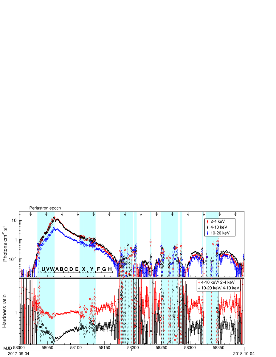
Figure 1: (Top) Background-subtracted X-ray light curves of Swift J0243.6 by the MAXI GSC in the 2–4 keV, 4–10 keV, and 10–20 keV bands. (Bottom) Time variations of two hardness ratios, 4–10 keV / 2-4 keV and 10–20 keV / 4–10 keV. Arrows in the top panel represent the epochs of periastron every 27.6 d orbital period. The 13 GSC data intervals, U, V, W, A, B, C, D, E, X, Y, F, G, and H, defined in table 2, are also presented. In both panels, cyan strips represent the periods covered only by the degraded GSC units. Data marked with filled ($\bullet$) and open ($\circ$) circles are taken by the normal and degrade units, respectively.

Figure 1 reveals that the present X-ray activity started at around MJD 58025 (2017 September 29) and continued for over 1.5 years. The first outburst developed into the largest one with the highest peak intensity (25 photons cm^-2 s^-1 $\simeq 7$ Crab in 2–20 keV) and the longest duration ($\sim 150$ d). After this, several outbursts with lower peaks ($\lesssim 1$ photons cm^-2 s^-1) and shorter durations ($\lesssim 40$ d) followed. Their recurrence cycles do not synchronize with the 27.3-d orbital period. This means that they are classified into the giant (type-II) outbursts of Be XBPs (e.g. Reig, 2011).

In figure 2, we show the hardness-intensity diagrams (HIDs), ie. SC or HC versus 2–20 keV photon flux $\equiv I_{2-20}$, using 2-d bin data. As seen in figure 1, the periods covered by the normal GSC units, MJD 58062-58108 and MJD 58135-58165, are limited to the outburst decay phase, and they have a gap from MJD 58108 to 58135. We hence employed data taken by the degraded GSC units during the gap. To reduce their large statistical uncertainty, these data were averaged over 5-d time bin. The obtained HIDs for the SC and HC are largely represented by a negative intensity-hardness correlation when the intensity is high ($I_{2-20}\gtrsim 0.8$), and relatively constant hardness ratios when the intensity is low ($I_{2-20}\lesssim 0.8$). These features agree with those obtained from the NICER data (WMJ18).

The two HIDs in figure 2, though grossly similar, differ in details. In the very high-intensity region of $I_{2-20}\gtrsim 4.5$ which is just after the outburst peak, the SC changes little with $I_{2-20}$ but the HC changes significantly. During the intermediate region of $0.8\lesssim I_{2-20}\lesssim 4.5$, the change of SC becomes larger, but that of HC becomes smaller than those at $I_{2-20}\gtrsim 4.5$. In figure 2, the boundaries of these regions at $I_{2-20}=0.8$ and $4.5$ are marked by dashed lines.

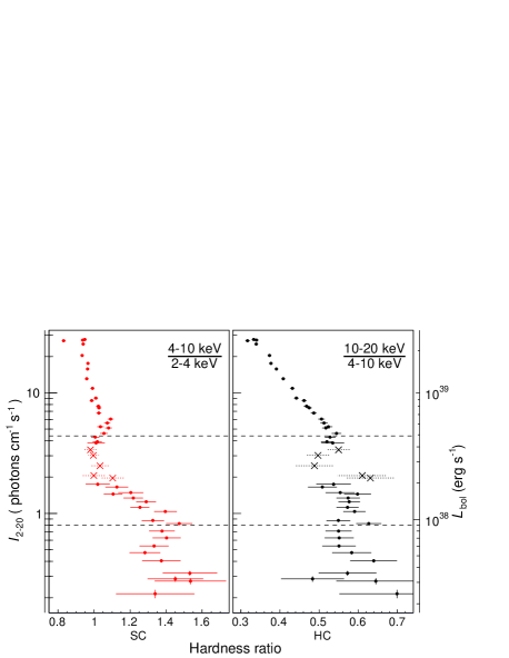
Figure 2: Hardness-intensity diagrams for the SC (left panel) and the HC (right panel). Data marked with crosses (X) were taken by the degraded GSC units. Dashed lines at $I_{2-20}=$0.8 and 4.5 represent the boundaries among three different regimes (see text). The right-side ordinate represents the bolometric luminosity calculated by assuming $D=7$ kpc, a bolometric correction factor in equation (4), and an isotropic emission.

To clarify the source evolution during the first outburst from MJD 58025 to 58175, we divided the time periods when Swift J0243.6 was observed by the normal GSC units into 8 intervals, and named them A through H, each covering 8–10 d, as illustrated in the top panel of figure 1. These intervals have gaps from the outburst start to MJD 58062, and from MJD 58106 to 58134, for which Swift J0243.6 was observed only by the degraded GSC units. We then decided to use the degraded units to fill in these two gaps, and divided them into 5 intervals, U through Y, each of which has a length of 8–14 d. Table 2 summarizes the start and stop time (MJD), the employed GSC units, exposure time ($T_{\mathrm{exp}}$), and average detector area ($A_{\mathrm{eff}}$) for the Swift J0243.6 direction in each interval. Below, we employ these interval definitions.

Table 2: The 13 GSC data intervals for the 2017-2018 outburst phase.

Int.	Start	Stop	GSC IDs	$T_{\mathrm{exp}}$ (s)	$A_{\mathrm{eff}}$ (cm2)
U	58038	58046	0,3,6	6115	0.981
V	58046	58054	0,3,6	10731	1.036
W	58054	58062	0,3,6	1516	1.140
A	58062	58070	1,4,7	2904	2.130
B	58070	58078	1,7	4819	3.097
C	58078	58086	1,7	5741	3.325
D	58086	58096	1,7	7102	3.287
E	58096	58106	1,7	5438	2.642
X	58106	58120	0,3,6	15333	0.933
Y	58120	58134	0,3,6	6962	0.852
F	58134	58144	1,4,7	3911	2.348
G	58144	58154	1,7	6535	3.243
H	58154	58164	1,7	7293	3.367

Note. — ^aStart and stop time in MJD. ^bThese intervals were covered by the degraded detector units.

3.2 Pulse profile evolution

To study time evolution of the pulsed X-ray emission, we performed pulse timing analysis. To begin with, every GSC event time was converted to that at the solar system barycenter. Then, these barycentric times were further corrected for the pulsar’s orbital motion, using the binary orbital parameters shown in table 1.

We examined the coherent pulsation, first with the GSC data. Considering the limited exposure and sparse time coverage, the epoch-folding period search was carried out for every 2-d interval. Figure 4 (a) shows the obtained pulse frequencies of the 2-d intervals for which the pulsation was detected significantly, from MJD 58038 to 58172 during the first giant outburst. The pulse frequency of Swift J0243.6 has also been measured by the Fermi/GBM on almost daily basis during the X-ray active periods. In figure 4 (a), the data from the Fermi/GBM are plotted together. We confirmed that the frequencies from the GSC data are all consistent with those of the Fermi/GBM within the errors quoted in the figure caption.

We then investigated pulse-profile evolution. To derive phase-coherent pulse profiles considering the pulse-period changes, we calculated a sequential pulse phase $\phi(t)$ for the event time $t$, as

$$\phi(t)=\int^{t}_{t_{0}}\nu(\tau)d\tau,$$ (1)

where $\nu(t)$ means the pulse-frequency time history, and $t_{0}$ is the phase-zero epoch, i.e. $\phi(t_{0})=0$. As $\nu(t)$ to represent the observations, we employed the daily frequencies taken by the Fermi/GBM at the measured time epochs, because they have better accuracies than those of the GSC. Also, $t_{0}$ was fixed at 58027.499066 (MJD), which is the epoch of the first Fermi/GBM periodicity detection. The behavior of $\nu(t)$ between adjacent data points was estimated by a cubic spline-fit model. In figure 4 (a), the interpolated $\nu(t)$ model is drawn on the data.

Using equation (1), we folded both the source and background light curves, normalized them to the average detector area for the source, and subtracted the latter from the former. In figure 4 (d), the pulse profiles obtained in this way every 2-d interval from MJD 58038 to 58172 are plotted in a 2-dimensional color image. Figures 4 (b) and 4 (c) show the pulse-phase-average X-ray flux and the root-mean-square (RMS) pulsed fraction, $f_{\mathrm{pul}}$ (WMJ18), calculated from each pulse profile. These figures reconfirm the sequential pulse-profile change reported by WMJ18.

Figure 4 (a) shows the pulse profiles averaged over the individual 8-14 d intervals of A through H, and U through Y, defined in table 2. The pulse profile changed from a double-peak shape in the brightest phase to a shallow single-peak one in the intermediate phase, and then to a dip-like feature developed in the fainter phase, as observed by NICER and Fermi/GBM (WMJ18).

Figure 4 (b) presents the $I_{2-20}$ dependence of $f_{\mathrm{pul}}$, calculated from the pulse profiles in figure 4 (a). We also produced pulse profiles in the hard band of 10–20 keV, with the same procedure. The $I_{2-20}$ dependence of $f_{\mathrm{pul}}$ in this band is plotted together in figure 4 (b). These results from the two bands confirm the NICER results (WMJ18) that the pulsed faction increase towards higher energies. The $f_{\mathrm{pul}}$ minimum at around $I_{2-20}\simeq 4.5$, corresponding to the epoch of transition from the double-peak to the single-peak, agrees well with the boundary of the two regimes in the HC-HID (right panel of figure 2).

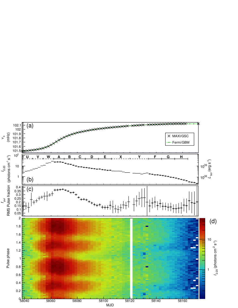
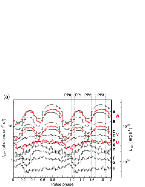
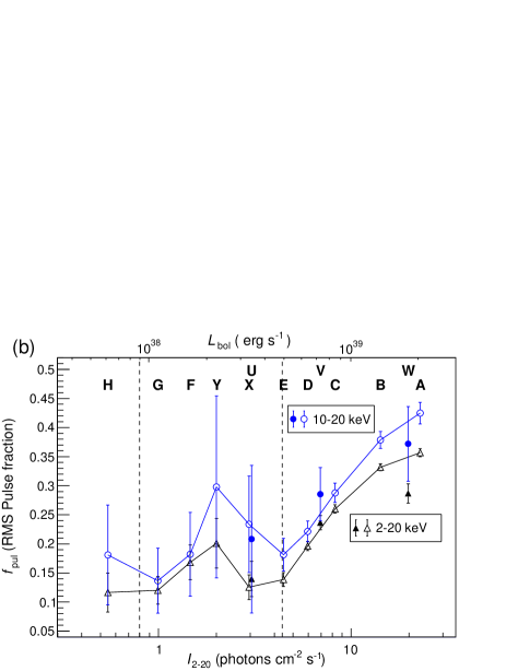
Figure 3: (a) The pulse frequency $\nu_{s}$ obtained with the GSC, and the Fermi/GBM. Solid line represents the cubic spline fits. Typical errors associated with the GSC and Fermi/GBM frequency determinations are $5\times 10^{-4}$ mHz and $5\times 10^{-6}$ mHz, respectively. (b) The 2-20 keV GSC photon flux $I_{2-20}$ averaged over the pulse phase. The ordinate on the right-side represents the luminosity scale, same as in figure 2. (c) RMS pulsed fraction $f_{\mathrm{pul}}$ of the 2-20 keV pulse profile. (d) Evolution of the 2-20 keV pulse profile in color coding from MJD 58040 to 58170.

Figure 4: (a) 2–20 keV pulse profiles for the individual intervals of A through H, and U through Y, defined in table 2. Profiles during the outburst rising (U, V, and W) are drawn in red and marked by crosses (X). Four pulse phases, PP0, PP1, PP2, and PP3, are defined at the top. (b) The $I_{2-20}$ dependence of $f_{\mathrm{pul}}$ in 2–20 keV (black circles) and 10–20 keV (blue triangles). Data in the rising phase are plotted with filled symbols (without lines). Vertical dashed lines represent the two $I_{2-20}$ boundaries characterizing the HIDs.

3.3 X-ray spectral evolution

3.3.1 Pulse-phase-average spectra

The source behavior on the HIDs, as seen in figures 1 and 2, suggests that the energy spectrum changed with the X-ray luminosity. We thus analyzed X-ray spectra taken with the GSC and averaged over the pulse phase. The spectral model fits were carried out on the XSPEC software version 12.8 (Arnaud, 1996) released as a part of the HEASOFT software package, version 6.25.

We extracted X-ray spectra for the 8 intervals, A through H, (table 2), which were observed by the normal GSCs units. Figure 5 (a) shows the obtained 2–30 keV spectra, where the background has been subtracted as described in section 2, but the instrumental responses are inclusive. To clarify the spectral evolution, we plot in figure 5 (b) their ratios to the spectra expected for a power-law function with a photon index $\Gamma=2$, i.e. $F(E)=E^{-2}$ (photons cm^-2 s^-1 keV^-1). The ratios confirm the softening with the flux increase, as seen in the HIDs (figure 2). In addition, the ratios are generally more convex than the $\Gamma=2$ power-law, with a mild bending at 6–8 keV. An enhancement at around 6.5 keV is considered to include the iron-K line emission.

As inspired by figure 5 (b), we fitted these spectra with a model composed of a high-energy-cutoff power-law (HECut) and a Gaussian (Gaus) for the iron-K emission line. The HECut model is represented by a photon index $\Gamma$, a cutoff energy $E_{\mathrm{cut}}$. a folded energy $E_{\mathrm{fold}}$, and a normalization factor $A$, as a function of the photon energy $E$ as

$$F_{\mathrm{HECut}}=\left\{\begin{array}[]{ll}AE^{-\Gamma}&(E\leq E_{\mathrm{cut}})\\ AE^{-\Gamma}\exp\left(-\frac{E-E_{\mathrm{cut}}}{E_{\mathrm{fold}}}\right)&(E_{\mathrm{cut}}<E).\end{array}\right.$$ (2)

The model has been successfully fitted to the spectra of major XBPs (e.g. White et al., 1983; Coburn et al., 2002). Because of the limited GSC energy resolution, we constrained the Gaussian centroid in a 6.4–7.0 keV range, and fixed the width at $\sigma=0.3$ keV, referring to the spectra of the typical XBPs. To account for the interstellar absorption, the continuum model was multiplied by a photoelectric absorption factor by a medium with the Solar abundances (Wilms et al., 2000), with the equivalent-hydrogen column density fixed at the Galactic HI density in the direction, $N_{\mathrm{H}}=0.7\times 10^{22}$ cm^-2 (Kalberla et al., 2005). This $N_{\mathrm{H}}$ value is consistent with that determined by the NuSTAR spectrum in the outburst early phase (Jaisawal et al., 2018). The model is hence expressed as tbabs*(powerlaw*highecut+gaussian) in the XSPEC terminology.

Figure 6 (a) shows the unfolded $\nu F\nu$ spectra of the A through H intervals together with their best-fit HECut$+$Gaus models, and figure 6 (b) shows individual data-to-model ratios. Table 3 summarizes the best-fit model parameters which include the absorption-corrected 0.5–60 keV flux, $F_{0.5-60}$, considered to approximate the bolometric flux. The value of $F_{0.5-60}=38$ erg cm^-2 s^-1 in the interval A corresponds to the bolometric luminosity $L_{\mathrm{bol}}=2.2\times 10^{39}$ erg s^-1 assuming an isotropic emission and $D=7$ kpc. Although the HECut$+$Gaus model largely reproduced the data, the data-to-model ratios are not always consistent with 1. The discrepancies are evident in higher-luminosity intervals and in energies $\gtrsim 6$ keV. The $\chi^{2}_{\nu}$ values indicate that the fits are not acceptable within the 95 % confidence limits in the first half of the observation, the intervals A through D, but those of the the second half, E to H, are acceptable.

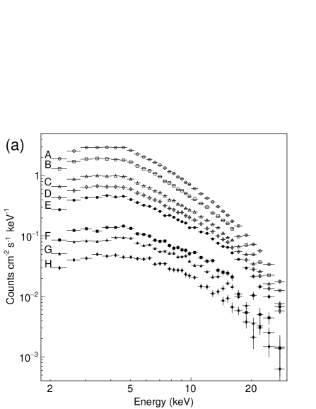
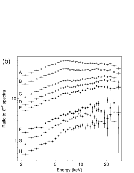
Figure 5: (a) The 2-30 keV GSC spectra for the intervals A through H, covering the outburst decay phase. The backgrounds have been subtracted, but the instrument responses are inclusive. (b) Ratios of the spectra in panel (a) to those expected for a power-law model $F(E)=E^{-2}$ (photons cm^-2 s^-1 keV^-1).

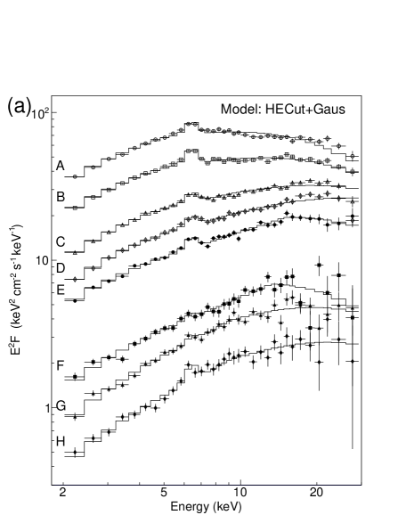
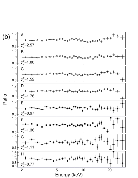
Figure 6: (a) Unfolded $\nu F\nu$ spectra and the best-fit HECut+Gaus models for the intervals, A to H. (b) Ratios of the observed spectra to the best-fit HECut+Gaus models.

Table 3: The best-fit spectral parameters with the HECut+Gaus and NPEX+Gaus models.

	Model: HECut + Gaus
	$A$	$\Gamma$	$E_{\mathrm{cut}}$	$E_{\mathrm{fold}}$	$E_{\mathrm{Fe}}$a	$EW_{\mathrm{Fe}}$b	$I_{\mathrm{2-20}}$c	$F_{\mathrm{0.5-60}}$d	$f_{\mathrm{bol}}$e	$\chi^{2}_{\nu}(\nu)$
Int.			(keV)	(keV)	(keV)	(eV)
A	$32^{*}$	$~{}1.52^{*}$	$~{}5.2^{*}$	$19^{*}$	$~{}6.4^{*}$	$170^{*}$	$25.3^{*}$	$37.9^{*}$	$~{}1.50^{*}$	2.66 (28)
B	$20^{+1}_{-1}$	$~{}1.50^{+0.03}_{-0.03}$	$~{}4.8^{+0.5}_{-0.5}$	$24^{+2}_{-2}$	$~{}6.4^{+0.03}_{-0.00}$	$210^{+40}_{-30}$	$16.2^{+0.1}_{-0.1}$	$26.0^{+0.5}_{-0.4}$	$~{}1.61^{+0.04}_{-0.04}$	1.95 (28)
C	$~{}9.1^{+0.4}_{-0.2}$	$~{}1.41^{+0.04}_{-0.04}$	$~{}4.2^{+0.8}_{-0.7}$	$32^{+5}_{-4}$	$~{}6.4^{+0.11}_{-0.00}$	$120^{+40}_{-40}$	$~{}8.74^{+0.06}_{-0.06}$	$15.9^{+0.4}_{-0.4}$	$~{}1.82^{+0.06}_{-0.06}$	1.58 (28)
D	$~{}5.6^{+0.4}_{-0.3}$	$~{}1.35^{+0.05}_{-0.05}$	$~{}3.8^{+1.7}_{-1.3}$	$40^{+11}_{-7}$	$~{}6.4^{+0.14}_{-0.00}$	$120^{+40}_{-30}$	$~{}6.05^{+0.04}_{-0.04}$	$12.1^{+0.4}_{-0.4}$	$~{}2.01^{+0.08}_{-0.08}$	1.82 (28)
E	$~{}4.5^{+0.17}_{-0.16}$	$~{}1.46^{+0.02}_{-0.02}$	$15^{+3}_{-4}$	$28^{+27}_{-11}$	$~{}6.4^{+0.12}_{-0.00}$	$140^{+50}_{-40}$	$~{}4.36^{+0.05}_{-0.05}$	$~{}8.4^{+0.8}_{-0.7}$	$~{}1.92^{+0.21}_{-0.17}$	1.01 (28)
F	$~{}1.11^{+0.09}_{-0.09}$	$~{}1.29^{+0.05}_{-0.05}$	$12.7^{+2.4}_{-2.5}$	$18^{+18}_{-8}$	$~{}6.4^{+0.6}_{-0.0}$	$40^{+90}_{-40}$	$~{}1.40^{+0.03}_{-0.03}$	$~{}2.5^{+0.5}_{-0.3}$	$~{}1.82^{+0.39}_{-0.27}$	1.44 (28)
G	$~{}0.57^{+0.05}_{-0.05}$	$~{}1.12^{+0.06}_{-0.07}$	$~{}9.0^{+2.0}_{-2.1}$	$22^{+9}_{-5}$	$~{}6.4^{+0.6}_{-0.0}$	$40^{+120}_{-40}$	$~{}0.93^{+0.02}_{-0.02}$	$~{}1.90^{+0.22}_{-0.18}$	$~{}2.03^{+0.27}_{-0.23}$	1.15 (28)
H	$~{}0.29^{+0.04}_{-0.03}$	$~{}1.09^{+0.08}_{-0.08}$	$~{}8.9^{+2.4}_{-2.0}$	$24^{+20}_{-8}$	$~{}6.4^{+0.6}_{-0.0}$	$210^{+140}_{-130}$	$~{}0.51^{+0.01}_{-0.01}$	$~{}1.09^{+0.21}_{-0.16}$	$~{}2.13^{+0.47}_{-0.36}$	0.80 (28)
	Model: NPEX + Gauss
	$A_{1}$	$\Gamma_{1}$	$A_{2}(\times 10^{3})$	$E_{\mathrm{fold}}$	$E_{\mathrm{Fe}}$a	$EW_{\mathrm{Fe}}$b	$I_{\mathrm{2-20}}$c	$F_{\mathrm{0.5-60}}$d	$f_{\mathrm{bol}}$e	$\chi^{2}_{\nu}(\nu)$
Int.				(keV)	(keV)	(eV)
A	$29^{*}$	$~{}1.04^{*}$	$~{}3.2^{*}$	$~{}7.2^{*}$	$~{}6.4^{*}$	$180^{*}$	$25.3^{*}$	$37.4^{*}$	$~{}1.48^{*}$	2.25 (28)
B	$18^{+1}_{-0}$	$~{}0.96^{+0.06}_{-0.04}$	$~{}5.3^{+2.6}_{-2.3}$	$~{}6.1^{+0.9}_{-0.6}$	$~{}6.4^{*}$	$210^{+30}_{-30}$	$16.2^{+0.1}_{-0.1}$	$24.5^{+0.9}_{-0.6}$	$~{}1.51^{+0.06}_{-0.05}$	1.55 (29)
C	$~{}8.5^{+0.4}_{-0.3}$	$~{}0.89^{+0.03}_{-0.03}$	$~{}5.1^{+1.6}_{-1.5}$	$~{}5.8^{+0.5}_{-0.4}$	$~{}6.4^{+0.15}_{-0.00}$	$130^{+40}_{-30}$	$~{}8.78^{+0.06}_{-0.06}$	$14.3^{+0.5}_{-0.4}$	$~{}1.63^{+0.06}_{-0.05}$	0.97 (28)
D	$~{}5.4^{+0.3}_{-0.2}$	$~{}0.86^{+0.03}_{-0.03}$	$~{}4.5^{+1.3}_{-1.2}$	$~{}5.8^{+0.5}_{-0.4}$	$~{}6.4^{+0.18}_{-0.00}$	$140^{+40}_{-30}$	$~{}6.10^{+0.05}_{-0.05}$	$10.5^{+0.4}_{-0.3}$	$~{}1.72^{+0.07}_{-0.06}$	1.24 (28)
E	$~{}4.0^{+0.4}_{-0.3}$	$~{}0.86^{+0.05}_{-0.05}$	$~{}5.1^{+1.9}_{-1.7}$	$~{}5.2^{+0.6}_{-0.4}$	$~{}6.4^{+0.16}_{-0.00}$	$140^{+70}_{-40}$	$~{}4.37^{+0.05}_{-0.05}$	$~{}7.4^{+0.4}_{-0.3}$	$~{}1.68^{+0.11}_{-0.08}$	1.09 (28)
F	$~{}1.32^{+0.32}_{-0.26}$	$~{}0.84^{+0.17}_{-0.15}$	$~{}4.7^{+2.5}_{-2.0}$	$~{}4.1^{+0.6}_{-0.4}$	$~{}6.4^{+0.6}_{-0.0}$	$90^{+150}_{-90}$	$~{}1.41^{+0.03}_{-0.03}$	$~{}2.2^{+0.2}_{-0.1}$	$~{}1.58^{+0.17}_{-0.13}$	1.51 (28)
G	$~{}0.49^{+0.06}_{-0.05}$	$~{}0.84^{+0.13}_{-0.15}$	$~{}0.00^{+0.04}_{-0.00}$	$17^{+7}_{-6}$	$~{}6.4^{+0.6}_{-0.0}$	$20^{+140}_{-20}$	$~{}0.93^{+0.02}_{-0.02}$	$~{}1.90^{+0.32}_{-0.18}$	$~{}2.03^{+0.38}_{-0.22}$	1.29 (28)
H	$~{}0.36^{+0.14}_{-0.10}$	$~{}0.71^{+0.25}_{-0.22}$	$~{}2.0^{+1.5}_{-2.0}$	$~{}4.0^{+1.1}_{-0.5}$	$~{}6.4^{+0.5}_{-0.0}$	$280^{+160}_{-150}$	$~{}0.52^{+0.01}_{-0.01}$	$~{}0.83^{+0.12}_{-0.07}$	$~{}1.61^{+0.28}_{-0.18}$	0.93 (28)

Note. — ^∗Errors are given with the 90% limits of statistical uncertainy if the fits are within the acceptable level ($\chi^{2}_{\nu}<2$).

^aCentroid and ^bequivalent width of iron-K line.

^cPhoton flux in 2-20 keV in photon cm^-2 s^-1.

^dAbsorption-corrected flux in 0.5-60 keV in $10^{-8}$ erg cm^-2 s^-1.

^eRatio of $I_{2-20}$ to $F_{0.5-60}$ in $10^{-8}$ erg photon^-1.

We then examined another continuum model, NPEX (Negative and Positive power laws with a common EXponential cutoff, Mihara et al., 1998), which has been used in the study of XBPs often more successfully than the HECut model. The NPEX model is represented by

$$F_{\mathrm{NPEX}}=\left(A_{1}E^{-\Gamma_{1}}+A_{2}E^{+\Gamma_{2}}\right)\exp\left(-\frac{E}{E_{\mathrm{fold}}}\right),$$ (3)

with five parameters, $\Gamma_{1}$, $\Gamma_{2}$, $A_{1}$, $A_{2}$, and $E_{\mathrm{fold}}$. We fixed $\Gamma_{2}(>0)$ at the typical value of 2.0 (Mihara et al., 1998). The best-fit NPEX+Gaus model parameters are listed in table 3. The fits have been improved, particularly when the source is luminous. However, the $\chi^{2}_{\nu}$ values are still unacceptable in the intervals A and B. In figure 7, the data-to-model ratios are presented. Above 10 keV, they still exhibit a feature that is similar to those in the HECut+Gaus model.

This characteristic excess feature has already been noticed in the NuSTAR and the NICER data (Tao et al., 2019; Jaisawal et al., 2019). There, it was considered as a “broad iron line”, and thus fitted with a Gaussian with $\sigma\sim 1.5$ keV. We hence attempted to fit the GSC spectra with a model consisting of an NPEX continuum, plus three Gaussians representing three lines at fixed energies of 6.4, 6.7 and 7.0 keV. The 6.4 keV line was allowed to take a free width, whereas the other two were assumed to be narrow. The fit was acceptable with $\chi^{2}_{\nu}=1.07$ (26 degree of freedom). The spectrum in the interval A (= outburst peak) gave the 6.4 keV width of $\sigma=1.27^{+0.27}_{-0.29}$ keV and the equivalent width of $EW_{\mathrm{Fe}}=0.54^{+0.20}_{-0.17}$ keV, which are consistent with those measured with NICER and NuSTAR spectra (Tao et al., 2019; Jaisawal et al., 2019).

Although the excess feature in the GSC spectra can be thus interpreted as a broad iron line, its origin is not necessarily clear (Jaisawal et al., 2019, also see later discussion). Therefore, other interpretations should be explored. The characteristic excess also reminds us of the “10 keV feature” that has been observed in several XBPs (e.g. Coburn et al., 2002), and interpreted either as a bump or an absorption on the cutoff power-law continuum (Klochkov et al., 2008). In the bump case, it can be fitted with a broad Gaussian (e.g. Müller et al., 2013; Reig & Nespoli, 2013) or a blackbody (hereafter BB) (Reig, & Coe, 1999). In the absorption case, it can look like a cyclotron-resonance absorption (CYAB; Mihara et al., 1990) We hence repeated the model fits by incorporating either a BB (bump case) or a CYAB model (absorption case) to the HECut or the NPEX continuum.

Table 4: The best-fit spectral parameters with the Cutoffpl+BB+Gaus and Cutoffpl*CYAB+Gaus models.

	Model: Cutoffpl + BB + Gaus
	$A$	$\Gamma$	$E_{\mathrm{fold}}$	$kT_{\mathrm{BB}}$a	$R_{\mathrm{BB}}$b	—	$E_{\mathrm{Fe}}$	$EW_{\mathrm{Fe}}$	$F_{\mathrm{0.5-60}}$	$f_{\mathrm{bol}}$	$\chi^{2}_{\nu}(\nu)$
Int.			(keV)	(keV)	(km)		(keV)	(eV)
A	$32^{+2}_{-2}$	$~{}1.63^{+0.10}_{-0.10}$	$49^{+70}_{-18}$	$~{}1.61^{+0.09}_{-0.10}$	$17^{+2}_{-2}$	—	$~{}6.4^{+0.12}_{-0.00}$	$120^{+50}_{-40}$	$41.3^{+1.7}_{-1.6}$	$1.64^{+0.08}_{-0.07}$	1.29 (27)
B	$18^{+1}_{-1}$	$~{}1.43^{+0.07}_{-0.06}$	$27^{+8}_{-5}$	$~{}1.34^{+0.14}_{-0.14}$	$14.0^{+3.2}_{-2.5}$	—	$~{}6.4^{+0.04}_{-0.00}$	$190^{+50}_{-30}$	$26.4^{+0.8}_{-0.7}$	$1.63^{+0.06}_{-0.05}$	1.48 (27)
C	$~{}7.8^{+0.8}_{-1.1}$	$~{}1.28^{+0.08}_{-0.10}$	$28^{+8}_{-6}$	$~{}1.08^{+0.21}_{-0.16}$	$13.6^{+7.1}_{-4.6}$	—	$~{}6.4^{+0.18}_{-0.00}$	$120^{+30}_{-50}$	$15.8^{+0.6}_{-0.6}$	$1.81^{+0.08}_{-0.08}$	1.27 (27)
D	$~{}4.9^{+0.8}_{-1.0}$	$~{}1.23^{+0.10}_{-0.15}$	$31^{+12}_{-8}$	$~{}0.94^{+0.36}_{-0.16}$	$12.3^{+10.1}_{-7.4}$	—	$~{}6.4^{+0.17}_{-0.00}$	$130^{+60}_{-40}$	$11.9^{+0.5}_{-0.6}$	$1.96^{+0.10}_{-0.11}$	1.74 (27)
	Model: Cutoffpl*CYAB + Gaus
	$A$	$\Gamma$	$E_{\mathrm{fold}}$	$E_{\mathrm{a}}$c	$W_{\mathrm{a}}$d	$D_{\mathrm{a}}$e	$E_{\mathrm{Fe}}$	$EW_{\mathrm{Fe}}$	$F_{\mathrm{0.5-60}}$	$f_{\mathrm{bol}}$	$\chi^{2}_{\nu}(\nu)$
Int.			(keV)	(keV)	(keV)		(keV)	(eV)
A	$28^{+1}_{-1}$	$~{}1.22^{+0.05}_{-0.05}$	$15^{+2}_{-1}$	$10.9^{+0.5}_{-0.7}$	$~{}3.7^{+1.6}_{-1.1}$	$~{}0.22^{+0.04}_{-0.04}$	$~{}6.4^{+0.09}_{-0.00}$	$110^{+40}_{-30}$	$37.5^{+0.3}_{-0.3}$	$1.48^{+0.02}_{-0.02}$	1.08 (26)
B	$18^{+1}_{-1}$	$~{}1.24^{+0.05}_{-0.05}$	$16^{+1}_{-1}$	$~{}9.5^{+0.6}_{-1.0}$	$~{}3.2^{+1.5}_{-1.1}$	$~{}0.14^{+0.03}_{-0.03}$	$~{}6.4^{+0.04}_{-0.00}$	$160^{+30}_{-30}$	$25.1^{+0.2}_{-0.2}$	$1.55^{+0.02}_{-0.02}$	1.13 (26)
C	$~{}8.4^{+0.5}_{-0.6}$	$~{}1.20^{+0.06}_{-0.09}$	$21^{+3}_{-3}$	$~{}8.5^{+0.9}_{-2.2}$	$~{}3.2^{+2.1}_{-1.4}$	$~{}0.12^{+0.04}_{-0.03}$	$~{}6.4^{+0.3}_{-0.0}$	$80^{+40}_{-40}$	$15.3^{+0.2}_{-0.2}$	$1.75^{+0.04}_{-0.03}$	0.98 (26)
D	$~{}5.4^{+0.3}_{-0.9}$	$~{}1.21^{+0.07}_{-0.36}$	$27^{+6}_{-9}$	$~{}8.2^{+1.7}_{-8.2}$	$~{}3.2^{+2.8}_{-1.5}$	$~{}0.08^{+0.06}_{-0.04}$	$~{}6.4^{+0.3}_{-0.0}$	$100^{+80}_{-50}$	$11.8^{+0.2}_{-0.2}$	$1.94^{+0.05}_{-0.04}$	1.63 (26)

Note. — ^∗Errors are given with the 90% limits of statistical uncertainy if the fits are within the acceptable level ($\chi^{2}_{\nu}<2$).

^aTemperature and ^bradius of BB emission assuming the distance $D=7$ kpc.

^cCyclotron-resonance energy, ^dwidth, and ^edepth in CYAB model.

Table 4 summarizes the best-fit parameters of these models for the A, B, C, and D spectra. Becuse $E_{\mathrm{cut}}$ in HECut or $A_{2}$ in NPEX was consistent with 0, the continuum in both models can be replaced by a simple cutoff power law (Cutoffpl) as $F_{\mathrm{Cutoffpl}}=A\exp(-E/E_{\mathrm{fold}})$. Therefore, the results are given in simple model forms as Cutoffppl+BB+Gaus and Cutoffpl*CYAB+Gaus. Figure 7 compares data-to-model ratios of the intervals A and B, when using the modeling of (1) HECut+Gaus, (2) NPEX+Gaus, (3) Cutoffpl+BB+Gaus, and (4) Cutoffpl*CYAB+Gaus. The fits are significantly improved by adding the BB or CYAB component. In the first two models of HECut+Gaus and NPEX+Gaus, the ratios show a dip-like structure at 6.4 keV, because the broad excess feature was fitted with a narrow Gaussian line. It was reduced in the latter two models. Figure 8 shows the implied Cutoffpl+BB+Gaus and Cutoffpl*CYAB+Gaus models that give the best fits to the interval-A spectrum.

While the latter two models are in the acceptable levels, their data-to-model ratios in figure 7 still seem to have a small ($\lesssim 3$ %) structure at around 5 keV. This is considered partly due to the systematic errors on the GSC response function, associated with the Xe-L edge at 4.8 keV (Mihara et al., 2011). We confirmed that the model-fit results did not change significantly even if its energy range (4.5-5.5 keV) was masked.

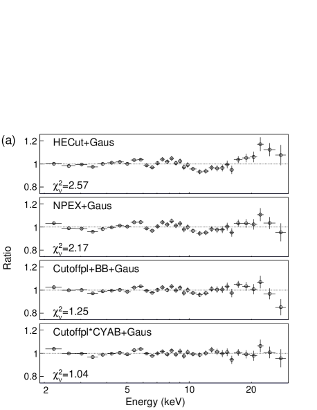
Figure 7: Ratios of the observed spectra for intervals A (panel a) and B (panel b) to the best-fit models with HECut+Gaus, NPEX+Gaus, Cutoffpl+BB+Gaus, and Cutoffpl*CYAB+Gaus, from the top to bottom panels. The best-fit $\chi^{2}_{\nu}$ value (in tables 3 and 4) are presented in each panel.

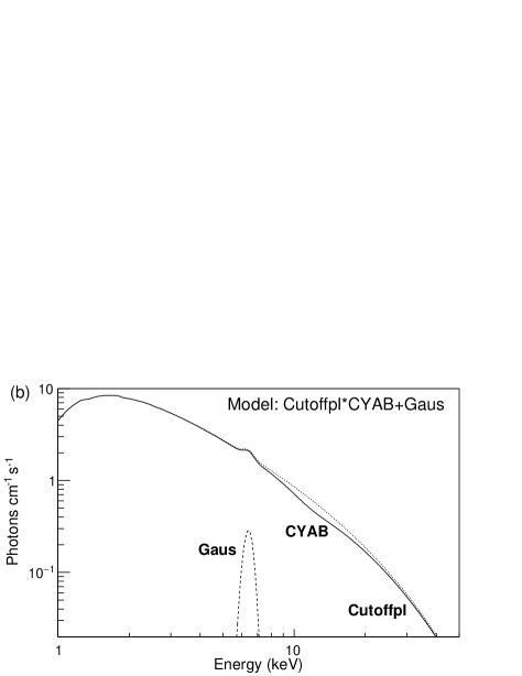
Figure 8: Two best-fit models for the interval-A spectrum, represented by (a) Cutoffpl+BB+Gaus and (b) Cutoffpl*CYAB+Gaus.

To visualize the spectral-parameter evolutions, figure 9 summarizes these best-fit parameters against the X-ray luminosity, where plotted are results with the HECut+Gaus, Cutoffpl+BB+Gaus, and Cutoffpl*CYAB+Gaus fits, that are acceptable within the 90% confidence limits. The power-law index $\Gamma$ increased with the luminosity, as expected from the negative correlation in the HIDs (figure 2). The Gaussian centroid for the iron line remained at $E_{\mathrm{Fe}}=6.4$ keV throughout the period. This appears inconsistent with the NuSTAR and NICER results that the narrow ($\sigma\lesssim 300$ eV) iron-line centroid shifted from 6.4 to 6.7 keV in the luminous regime over the Eddington limit (Tao et al., 2019; Jaisawal et al., 2019), but this discrepancy is because the GSC spectrum with the resolution $\Delta E\sim 0.8$ keV (at 6 keV) was dominated by the broad structure with a peak at $\sim 6.4$ keV. The equivalent width is almost constant at $EW_{\mathrm{Fe}}\sim 100$ eV, in agreement with the NICER result that the iron-line flux was approximately proportional to the luminosity (Jaisawal et al., 2019), as well as with the behavior of the typical XBPs (Reig & Nespoli, 2013). When the 10 keV feature is fitted with a BB model, the BB temperature increased from $kT_{\mathrm{BB}}\sim 1$ to 1.4 keV, but the BB radius did not change significantly from $R_{\mathrm{BB}}\sim 10$ km. When it is fitted with the CYAB absorption model, the CYAB energy and its width remained at $E_{\mathrm{a}}\sim 10$ keV and $W_{\mathrm{a}}\sim 3$ keV, respectively, but the depth increased from $D_{\mathrm{a}}\sim 0.1$ to $0.2$ with the luminosity.

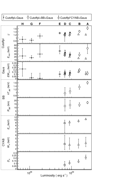
Figure 9: Dependence of the spectral parameters on the X-ray luminosity, obtained from the model fits to the interval A to H spectra with Cutoffpl+Gaus, Cutoffpl+BB+Gaus, and Cutoffpl*CYAB+Gaus. Error bars represent 90% confidence limits of the statistical uncertainties. Only those fits that are acceptable within the 90% confidence are shown.

3.3.2 Pulse-phase-resolved spectra

Pulse profiles obtained by NICER in 0.2–12 keV were little energy dependent during the luminous ($\gtrsim 2\times 10^{38}$ erg s^-1) period, but their pulsed fractions increased toward higher energies (WMJ18). As seen in section 3.2 (figure 4), the same trend was observed in the GSC 2-20 keV data. This suggests that the X-ray spectrum gets harder around the pulse peaks.

We hence extracted pulse-phase-resolved spectra for 4 pulse phases (PP) as illustrated in figure 4, which we hereafter call the minimum (PP1), the intermediate high (PP2), the intermediate low (PP3), and the maximum (PP4), respectively, in the double-peak profile. Figure 10 shows the ratios of each phase-resolved spectrum to the entire phase average during the luminous period of the intervals A, B, C, and D. It confirms that the pulsed fraction indeed increases toward higher energies. We also performed the model fit to the individual pulse-phase spectra, but were not able to find significant phase-dependent parameter changes except for the power-law index $\Gamma$ and the emission normalization.

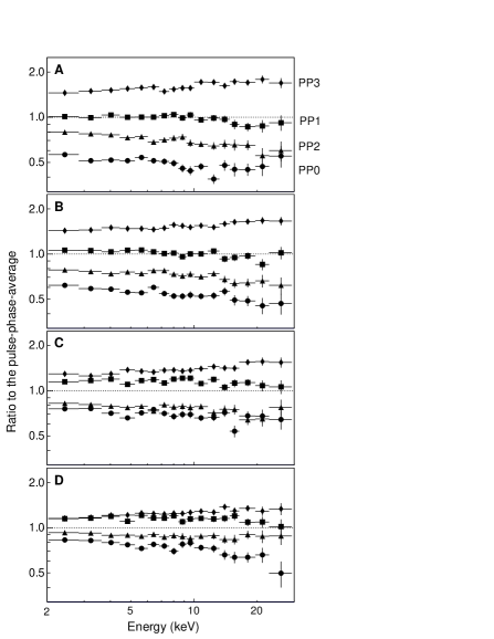
Figure 10: Ratios of the pulse-phase-resolved spectra for PP0, PP1, PP2, and PP3 to that of the pulse-phase average in the same interval. Penels A, B, C, and D, represents the spectra from the time intervals A to D, respectively.

3.4 Luminosity - spin-up relation

As seen in figure 4, the spin-frequency increase, i.e. the pulsar spin up, is closely correlated with the X-ray intensity. Although correlation was already reported by Doroshenko et al. (2018) and Zhang et al. (2019), we here refine the analysis by jointly using the MAXI GSC light curve and the Fermi GBM pulse period. These data have an advantage that both are available almost with a daily sampling.

For the above purpose, we need to convert $I_{2-20}$ to the bolometric luminosity $L_{\mathrm{bol}}$. The bolometric correction factor $f_{\mathrm{bol}}=F_{0.5-60}/I_{2-20}$, used in this conversion, depends on the energy spectrum. Figure 11 shows the relation between $I_{2-20}$ and $F_{0.5-60}$ calculated from the best-fit spectral models in tables 3 and 4. Although the values of $F_{0.5-60}$ depend to some extent on the fitting models, the effect is within the statistical uncertainties ($\lesssim 10\%$). The factor $f_{\mathrm{bol}}$ slightly decreases towards the higher $I_{2-20}$, according to the spectral softening as observed in the HID (figure 2). Based on the HID behavior, we assumed that the $f_{\mathrm{bol}}$-$I_{2-20}$ relatioin can be expressed as

$$f_{\mathrm{bol}}=\left\{\begin{array}[]{ll}f_{0}&(I_{2-20}<4.5)\\ f_{0}\left(I_{2-20}/4.5\right)^{-\gamma}&(I_{2-20}>4.5),\end{array}\right.$$ (4)

which is constant at $f_{0}$ in $I_{2-20}<4.5$ where HC is constant, and decreases by a power-law in $I_{2-20}>4.5$. We fitted equation (4) to the $f_{\mathrm{bol}}$-$I_{2-20}$ data obtained from the NPEX spectral parameters, and determined the best-fit values of $f_{0}=1.74\times 10^{-8}$ erg photon^-1, and $\gamma=0.10$. The scale of $L_{\mathrm{bol}}$ in figures 2, 4, 4 (a), and 4 (b), associated with $I_{\mathrm{2-20}}$, have been calculated by $L_{\mathrm{bol}}=4\pi D^{2}I_{2-20}f_{\mathrm{bol}}$ and $D=7$ kpc.

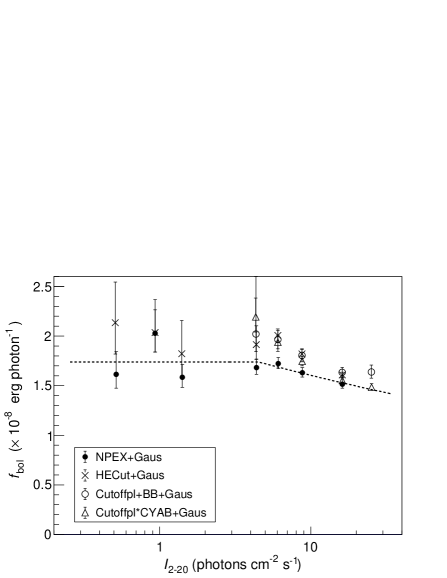
Figure 11: Relation between $f_{\mathrm{bol}}=F_{0.5-60}/I_{2-20}$ and $I_{2-20}$, calculated from the best-fit models for the A through H spectra in tables 3 and 4. Dashed line represents the best-fit function to the NPEX-model data with equation (4).

Figure 12 shows the obtained $\dot{\nu}_{\mathrm{s}}$-$L_{\mathrm{bol}}$ relation, where we calculated the spin-frequency derivative $\dot{\nu}_{\mathrm{s}}$ from the Fermi/GBM pulsar data with the same procedure as in Sugizaki et al. (2017). It clearly reveals a positive correlation close to the proportionality. We fitted the data points with a power-law, $\dot{\nu}_{\mathrm{s}}\propto L_{\mathrm{bol}}^{\alpha}$, and obtained the best-fit power-law index $\alpha=1.0~{}(\pm 0.02)$, where the fitting error is estimated by adding appropriate systematic errors so as to make the fit formally acceptable. The best-fit $\alpha$ value is somewhat higher than those of the theoretical predictions, $6/7$ in Ghosh & Lamb (1979, hereafter GL79), $0.85$ in Lovelace et al. (1995), and $0.9$ in Kluźniak & Rappaport (2007), but agrees with the empirical relations determined from the observed data of major Be XBPs (Bildsten et al., 1997; Sugizaki et al., 2017).

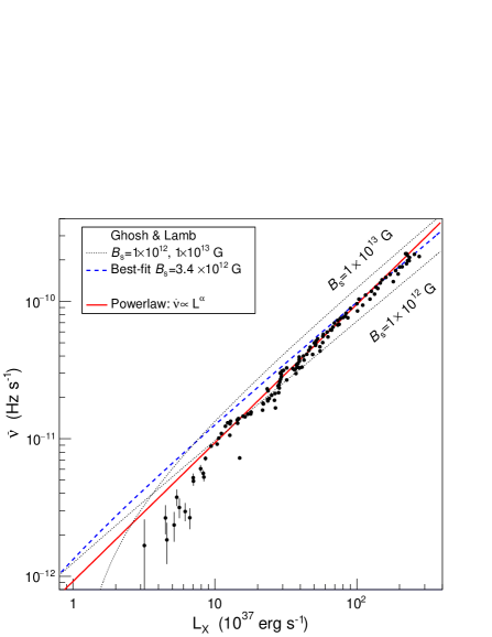
Figure 12: The observed relation between $L_{\mathrm{bol}}$ and $\dot{\nu}_{\mathrm{s}}$. The dotted lines represent the GL79 models for surface magnetic field $B_{\mathrm{s}}=1\times 10^{12}$ and $1\times 10^{13}$ G. The red-solid and blue-dashed lines represent the best-fit power-law and the best-fit GL79 model, respectively.

We also compared the coefficient of proportionality between $\dot{\nu}_{\mathrm{s}}$ and $L_{\mathrm{bol}}$, with those of the theoretical models. Specifically, the date in figure 12 are compared with the relations predicted by the representative GL79 model, assuming the canonical neutron-star mass $1.4M_{\odot}$, the radius 10 km, the moment of inertial $10^{45}$ g cm², and the typical surface-magnetic fields $B_{\mathrm{s}}=1\times 10^{12}$ and $1\times 10^{13}$ G. Although the data and the models slightly disagree in $\alpha$, the data are mostly distributed between the two model curves. This means that the data prefer $B_{\mathrm{s}}$ between these two values, i.e. a few $\times 10^{12}$. The best-fit GL79 model suggests $B_{\mathrm{s}}=3.4\times 10^{12}$ G.

4 Discussion

The MAXI GSC data of Swift J0243.6, during the giant outburst from 2017 October to 2018 January, revealed the complex behavior in the X-ray spectrum as well as the pulse profile. Based on these results, we consider possible scenarios of the X-ray emission evolution, particularly at around the peak where the luminosity exceeded the Eddington limit by up to a factor of $\gtrsim 10$. Also, comparing the behavior with those of other Be XBPs and ULXPs, we discuss what causes the extraordinary super-Eddington emission of this object.

4.1 Relations between spectral and pulse-profile transitions

The simultaneous changes in the X-ray spectrum and the pulse profile of Swift J0243.6 have been noticed in the NICER and Fermi/GBM data (WMJ18). However, possible relations between the two attributes have not been necessarily clear, because of their uneven time coverage. We here study this issue by using the MAXI GSC results.

As shown in figure 2, during the remarkable X-ray active period of $I_{2-20}\gtrsim 0.8$, the two hardness rations, the SC and HC, both showed a negative correlation against $I_{2-20}$. According to the simple HID classification (Reig, 2008), it is classified into the diagonal branch (DB), and the part of $I_{2-20}\lesssim 0.8$ is thought to be the horizontal branch (HB) from the result of NICER (WMJ18). However, the two HIDs employing SC and HC show characteristic differences in the DB. We hence divide the DB region into the follwoing two states, (i) the intermediate DB state of $0.8\lesssim I_{2-20}\lesssim 4.5$ where the SC changed more than HC, and (ii) the extreme DB state of $I_{2-20}\gtrsim 4.5$ where the HC changed more than SC. Using $f_{\mathrm{bol}}$ in equation 4, these characteristic intensities of $I_{2-20}=0.8$ and $4.5$ correspond to the luminosities of $L_{\mathrm{bol}}=0.9\times 10^{38}$ and $5\times 10^{38}$ erg s^-1, respectively.

The spectral analysis clarified how the 2–30 keV spectrum changed between the two DB states. Generally, X-ray spectra of Be XBPs are represented with a Cutoffpl continuum (Makishima et al., 1999; Coburn et al., 2002), where their luminosity-dependent changes in the DB are characterized by a correlation between $L_{\mathrm{bol}}$ and $\Gamma$ (Reig & Nespoli, 2013). As shown in figure 9, the best-fit parameters obtained from Swift J0243.6 exhibit this general behavior. In the extreme DB state (intervals A, B, C, and D), the increased 6 keV excess on top of the Cutoffpl continuum, further enhanced the change in the HC, but reduced the change in the SC.

The pulse-profile evolution in figures 4 and 4 also suggests that it is related with the two DB states, because transition between the single-peak and double-peak occurred at $I_{2-20}\simeq 4.5$, just at the boundary of the two DB states. These correlated changes in the spectrum and the pulse profile are considered to reflect luminosity-related changes in the physical condition of the X-ray emission region. Table 5 summarizes how the spectral and temporal properties depend on the X-ray intensity.

Table 5: Luminosity-dependent changes in the X-ray properties

HID branch	HB		DB
Sub state in DB			Intermed.		Extreme
$I_{2-20}$a		0.8		4.5		30
$L_{\mathrm{bol}}$ ($10^{38}$)b		0.9		5.0		26
Intervalc	H	G F (Y X)		E D C B A
SC-$I_{2-20}$ sloped	$+$($\nearrow$)		$-$($\searrow$)		$\sim$$0$ ($\rightarrow$)
HC-$I_{-20}$ sloped	$+$($\nearrow$)		$\sim$$0$ ($\rightarrow$)		$-$($\searrow$)
Spec. profile	Cutoffpl + Iron-K line				+ $\gtrsim 6$ keV excess
Pulse profile	Single-peak				Double-peak

Note. — ^a 2–20 keV photon flux (photons cm^-2 s^-1).

^b Bolometric luminosity (erg s^-1).

^c GSC data intervals defined in table 2.

^d $+$($\nearrow$) means positive correlation, and ($\searrow$) negative correlation, and $\sim$$0$($\rightarrow$) means little dependence.

4.2 X-ray emission in the super-Eddington regime

As discussed above, the X-ray spectrum of Swift J0243.6 in the extreme DB state is characterized by the excess at $\gtrsim 6$ keV. Because the feature can be represented by a Gaussian function with the centroid $\sim 6.4$ keV and the width $\sigma\sim 1.2$ keV, Jaisawal et al. (2019) interpreted it as a broad iron-K line. However, a question about what cause such a broad iron line has not been answered. The broad Gaussian model also needs to have a large equivalent width of $\sim 1$ keV (Tao et al., 2019; Jaisawal et al., 2019), which would be realized only when the direct X-ray component is suppressed by source obscuration. However, such an obscuration feature has not been observed. Meanwhile, to explain the power spectrum obtained from the insight-HXMT data during the DB period, Doroshenko et al. (2020) proposed a scenario that the major X-ray emission came from an accretion disk, which made transition from a state dominated by Coulomb collisions to that by radiation. However, the picture is also considered difficult from the pulsed fraction evolution, which increased up to $\gtrsim 40$% (RMS amplitude) in proportion to the luminosity. Furthermore, an accretion disk in a XBP must be truncated at the magnetospheric radius, or so-called Alfven radius (Ghosh & Lamb, 1979), $R_{\mathrm{A}}=1400L_{\mathrm{38}}^{-2/7}M_{1.4}^{1/7}R_{6}^{10/7}B_{12}^{4/7}\,\mathrm{km}$, where $L_{38}$, $M_{1.4}$, $R_{6}$ and $B_{12}$ are the source luminosity in $10^{38}$ erg s^-1, neutron-star mass in $1.4M_{\odot}$, radius in $10^{6}$ cm, and surface magnetic field in $10^{12}$ G. Therefore, the specific gravitational energy which the accreting matter acquires throughout the disk would be two order of magnitude smaller than is available by the time it reaches the neutron-star surface. In other words, the disk would not provide a major source for the observed pulsed hard X-rays. The absorption line detected with the Chandra HETGS can be explained without invoking an X-ray emitting disk, because the strong radiation pressure would produce outflows from the cool disk outside $R_{\mathrm{A}}$, or from the accretion stream inside $R_{\mathrm{A}}$. Hence, we consider another interpretation for these spectral and pulse-profile behavior.

As shown in figure 7, the MAXI GSC spectra with the excess feature can be fitted if either a bump represented by a BB or an absorption by a CYAB model is incorporated into the HECut or NPEX continuum. These model parameters are consistent with those for the ”10 keV feature” which has been reported previously in several XBPs (e.g. Coburn et al., 2002; Klochkov et al., 2008). Also, similar spectral and pulse-profile changes have been observed in several Be XBPs, 4U 0115$+$63 (Ferrigno et al., 2009), X 0331$+$53 (Tsygankov et al., 2010), EXO 2030$+$375 (Epili et al., 2017), and SMC X-3 (Weng et al., 2017), when close to the Eddington limit. These facts imply that the behavior is not unique to Swift J0243.6, but common to the other XBPs.

Based on the canonical models of X-ray emission from XBPs (e.g. Basko & Sunyaev, 1976; Becker et al., 2012), these X-rays are considered to originate from accretion columns that are formed on the neutron star surface through the magnetic filed lines. In this scenario, the two HID branches, HB and DB, are thought to represent two accretion regimes where accreting matter flows are decelerated by Coulomb collisions (sub-critical accretion regime) and radiation pressure (super-critical accretion regime), respectively. The spectral softening in the DB is interpreted by a development of Comptonized emission in the accretion columns. As the luminosity increases, the region responsible for the Comptonization extends farther from the neutron star surface, and then the temperature of the Comptonizing plasma decreases. The scenario also explains the pulsed emission evolution (Basko, & Sunyaev, 1975; Becker et al., 2012). Theoretically (Becker et al., 2012), the emission column height $h_{\mathrm{s}}$ is expected to be proportional to $L_{\mathrm{bol}}$ in the supercritical regime, until it reaches a few km at the Eddington luminosity. When $h_{\mathrm{s}}$ becomes larger than the column radius $r_{\mathrm{c}}$ ($\sim 1$ km), the pulsed emission geometry changes from pencil beam to fan beam, which results in the transition from the single-peak to the double-peak pulse profile. Furthermore, if $h_{\mathrm{s}}\gg r_{\mathrm{c}}$, the pulsed fraction tends to be approximately proportional to $h_{\mathrm{s}}$, and thus to $L_{\mathrm{bol}}$. The observed correlation between $f_{\mathrm{pul}}$ and $I_{2-20}$ in figure 4 (b) agrees with this prediction.

Then, what produces the 6 keV excess in the extreme DB state? When the BB bump model is employed, the change of the feature with $L_{\mathrm{bol}}$ is represented by the BB temperature, which increased from $kT_{\mathrm{BB}}=1.0$ to 1.6 keV. On the other hand, the BB radius was almost constant at $R_{\mathrm{BB}}\sim 10$ km. Assuming that the BB emission came from the accretion column of $r_{\mathrm{c}}\sim 1$ km, its height need to be $h_{\mathrm{s}}\sim 100$ km to attain the BB area $=\pi R_{\mathrm{BB}}^{2}\sim 100$ km². The estimated $h_{\mathrm{s}}$ seems too high compared with the theoretical prediction of a few km. This difficulty would not be solved even if we consider significant temperature gradient in the emission region.

Alternatively, assuming the CYAB interpretation, we obtained the best-fit parameters as $E_{\mathrm{a}}\simeq 10$ keV, $W_{\mathrm{a}}\simeq 3$ keV, and $D_{\mathrm{a}}\simeq 0.1-0.2$. Compared with other XBPs (e.g. Makishima et al., 1999; Coburn et al., 2002), the values of $E_{\mathrm{a}}$ and $D_{\mathrm{a}}$ are at the lower ends of their distributions, but still within their observed ranges. The value of $W_{\mathrm{a}}$ is typical. Therefore, the CYAB parameters are not so unusual. In this scenario, $E_{\mathrm{a}}=10$ keV means $B_{\mathrm{s}}=0.86(1+z_{\mathrm{g}})\times 10^{12}\simeq 1.1\times 10^{12}$ G, where $z_{\mathrm{g}}$ represents the gravitational redshift. This estimate is consistent with the implication of figure 12. On the other hand, the $L_{\mathrm{bol}}$ dependence of the parameters, including an increase of $D_{\mathrm{a}}$ from 0.1 to 0.2, and relatively constant values of $E_{\mathrm{a}}$ and $W_{\mathrm{a}}$, are not necessarily typical of the cyclotron resonance effects in other XBPs, where $D_{\mathrm{a}}$ is relatively constant and $E_{\mathrm{a}}$ often decrease towards high $L_{\mathrm{bol}}$ (e.g. Mihara et al., 2004). Therefore, we retain this interpretation as a possible candidate.

4.3 Surface magnetic field

The surface magnetic field $B_{\mathrm{s}}$ is one of the key parameters of the accretion process. In the section above, we arrived at a possibility of $B_{\mathrm{s}}\simeq 1.1\times 10^{12}$ G, assuming that the 6 keV excess feature in the spectrum of the extreme DB state is a result of a cyclotron-resonance absorption at $\sim 10$ keV. Meanwhile, several other attempts to constrain $B_{\mathrm{s}}$ have been performed, so far. Tsygankov et al. (2018) derived $B_{\mathrm{s}}<1\times 10^{13}$ G from the upper limit on the propeller luminosity. An estimate of $0.1-2\times 10^{13}$ G was derived by WMJ18 from the HID transition luminosity and the QPO frequency. From the correlated X-ray flux and spin-up evolution observed by the insight-HXMT, Zhang et al. (2019) estimated $B_{\mathrm{s}}\sim 1\times 10^{13}$ G. While all these constraints are consistent, they have large uncertainties which stem from those in the theoretical relations employed to interpret the observed data. As a result, these published reports enable us to neither assess the reality of our cyclotron hypothesis, nor examine whether $B_{\mathrm{s}}$ of Swift J0243.6 is different from those of typical XBPs.

We also studied this subject using the $\dot{\nu}_{\mathrm{s}}$-$L_{\mathrm{bol}}$ relation from the MAXI/GSC and Fermi/GBM data (section 3.4), and found that the positive correlation between the two quantities smoothly extends up to the maximum luminosity, $L_{\mathrm{bol}}\gtrsim 2\times 10^{39}$ erg s^-1 (figure 12). Assuming the neutron-star mass $1.4M_{\odot}$, the radius of 10 km, and the GL79 disk-magnetosphere interaction model, the data are best explained with $B_{\mathrm{s}}\simeq 3.4\times 10^{12}$ G. Although the model largely reproduce the data, the fit is not as good as being acceptable. The discrepancy is considered mainly on the assumed physical conditions in GL79, which is estimated to affect the coefficient of proportionality between $\dot{\nu}_{\mathrm{s}}$ and $L_{\mathrm{bol}}$ by a factor of $\sim 2$ (e.g. Bozzo et al., 2009). In fact, Sugizaki et al. (2017) confirmed that the GL79 model reproduced the observed $\dot{\nu}_{\mathrm{s}}$-$L_{\mathrm{bol}}$ relations of 12 Be XBPs with an accuracy of a factor $\lesssim 3$.

To avoid these model uncertainties, we compare, in figure 13, the observed $\dot{\nu}_{\mathrm{s}}$-$L_{\mathrm{bol}}$ relation of Swift J0243.6 with those of other Be XBPs of which $B_{\mathrm{s}}$ is determined by the cyclotron-resonance feature. These are the 9 Be XBPs in Sugizaki et al. (2017); 4U 0115$+$63, X 0331$+$53, RX J0520.5$-$6932, H 1553$-$542, XTE J1946$+$274, KS 1947$+$300, GRO J1008$-$57, A 0535$+$262, and GX 304$-$1. The results for these XBPs have been derived from the MAXI/GSC and Fermi/GBM data in the same way as for Swift J0243.6. The values of $L_{\mathrm{bol}}$ of 4 objects, 4U 0115$+$63, X 0331$+$53, A 0535$+$262, and GX 304$-$1, have been revised, using the updated $D$ in the GAIA DR2. (These changes in $D$ from the values employed by Sugizaki et al. (2017) are $<15$%.) Except for one outlier, X 0331$+$53, the $\dot{\nu}_{\mathrm{s}}$-$L_{\mathrm{bol}}$ relations of these objects all line up within a factor of $\sim 3$. The data of Swift J0243.6 locate almost at the bottom of them, in agreement with the fact that the best-fit GL79 model implies the lowest $B_{\mathrm{s}}$ among the known XBPs. The result suggests that $B_{\mathrm{s}}$ of Swift J0243.6 is not much different from the $B_{\mathrm{s}}$ range of XBPs, and tends to be relatively low. The timing analysis hence reinforce the cyclotron-absorption interpretation of the $\sim 6$ keV excess feature.

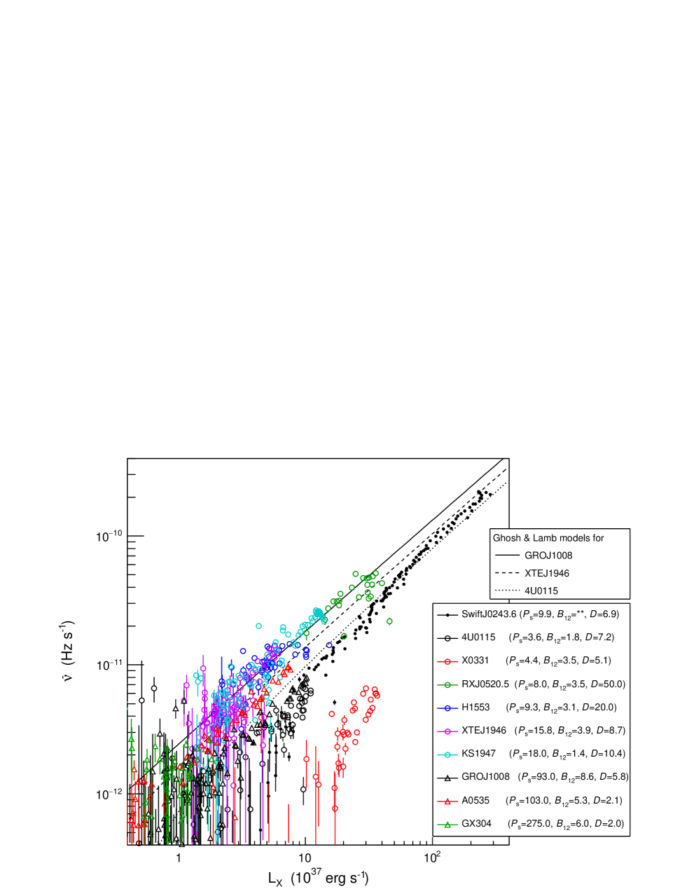
Figure 13: The observed $\dot{\nu}_{\mathrm{s}}$ versus $L_{\mathrm{bol}}$ relation of Swift J0243.6 (black dot), compared with those of other 9 Be XBPs (4U 0115$+$63, X 0331$+$53, RX J0520.5$-$6932, H 1553$-$542, XTE J1946$+$274, KS 1947$+$300, GRO J1008$-$57, A 0535$+$262, and GX 304$-$1) whose $B_{\mathrm{s}}$ is determined by the cyclotron feature. All the data were produced from the MAXI GSC light curves and the Fermi GBM pulsar data (Sugizaki et al., 2017). In the legend, the spin period $P_{\mathrm{s}}$ (s), the surface magnetic field $B_{12}$ (in $10^{12}$ G), and the assumed source distance $D$ (kpc) of each object are presented.

4.4 Comparison with other ULXPs

In our Galaxy, Swift J0243.6 is the first example of the ULXP, as well as the ULX. Therefore, the MAXI GSC results should give important hints about their unknown origins. Table 4.4 compares the basic parameters of Swift J0243.6 with those of the known 6 ULXPs, M82 X-2 (Bachetti et al., 2014), NGC 300 ULX-1 (Carpano et al., 2018), NGC 7793 P13 (Fürst et al., 2016), NGC 5907 ULX-1 (Israel et al., 2017), and SMC X-3 (Tsygankov et al., 2017), which have all been securely identified as ULXPs with the maximum luminosities $>2.5\times 10^{39}$ erg s^-1.

Table 6: Basic parameters of known ULX pulsars

Source name	$P_{\mathrm{spin}}$ (s)	$P_{\mathrm{orb}}$ (d)	$L_{\mathrm{max}}$ (erg s-1)	$D$ (Mpc)	Opt.	P/T	$B_{\mathrm{s}}^{\mathrm{su}}$ (G)	$B_{\mathrm{s}}^{\mathrm{pr}}$ (G)
NGC 5907 ULX-1∗1	1.14	5?	$6.0\times 10^{40}$	17	–	P	–	–
M82 X-2∗2	1.37	2.5	$2.0\times 10^{40}$	3.5	B9I	P	–	$\sim 1\times 10^{14}$
NGC 7793 P13∗3	0.42	64	$1.0\times 10^{40}$	3.9	–	P	$(1.5\times 10^{12}$)	–
NGC 300 ULX-1∗4	31.6	–	$5.0\times 10^{39}$	1.9	Be	T	$3\times 10^{12}$	–
SMC X-3∗5	7.8	45.1	$2.5\times 10^{39}$	0.062	Be	T	$2.6\times 10^{12}$	$(1-5)\times 10^{12}$
Swift J0243.6∗6	9.7	27.6	$2.5\times 10^{39}$	0.007	Be	T	$2.5\times 10^{12}$	$<6.2\times 10^{12}$

Note. — $P_{\mathrm{spin}}$ - spin period; $P_{\mathrm{orb}}$ - orbital period; $D$ - source distance; $L_{\mathrm{max}}$ - observed maximum luminosity; Opt. - optical counterpart; P/T - Persistent or Transient; $B_{\mathrm{s}}^{\mathrm{su}}$ - $B_{\mathrm{s}}$ from luminsity - spin-up relation; $B_{\mathrm{s}}^{\mathrm{pr}}$ - $B_{\mathrm{s}}$ from propeller effect.

References. — ^∗1Israel et al. (2017), ^∗2Bachetti et al. (2014); Tsygankov et al. (2016), ^∗3Fürst et al. (2016), ^∗4Carpano et al. (2018), ^∗5Tsygankov et al. (2017), ^∗6Tsygankov et al. (2018); WMJ18.

X-ray properties of XBPs depends considerably on the type of their mass-donating companions. The XBPs known in our Galaxy are mostly classified into those accompanied by supergiant primaries, i.e. Sg XBPs, and the Be XBPs (e.g. Reig, 2011; Walter et al., 2015) which have been a major focus of the present paper. While Sg XBPs show persistent X-ray activities often involving flare-like time variations, Be XBPs show mostly periodical outbursts lasting for a week to months (e.g. Bildsten et al., 1997). Out of the 6 ULXP sample, four have allowed optical identifications, and hence the classification; one Sg XBP and three Be XBPs. From the type of their X-ray activity, the remaining two are naturally considered to be Sg XBPs. Therefore, regardless of its optical companion type, any XBP may become, on certain conditions, an ULXP. In table 4.4, the ULXPs with Be companions are generally found to have longer $P_{\mathrm{s}}$, as well as longer $P_{\mathrm{orb}}$, than the objects of Sg companions, in agreement with those of the XBPs in our Galaxy (Corbet, 1986). This suggests that the binary evolution of the ULXPs are not much different from those of standard XBPs.

As the origin of the super-Eddington luminosity in ULXPs, a strong $B_{\mathrm{s}}$ reaching $\sim 10^{14}$ G has been proposed with a theoretical model (Mushtukov et al., 2015). However, it would be natured to presume that a stronger dipole filed would enlarge the Alfven radius and make it closer to the Bondi radius for gravitational capture of the accreting gas, thus suppressing the accretion. Actually, Yatabe et al. (2018) found, through the $\dot{\nu}_{\mathrm{s}}$-$L_{\mathrm{bol}}$ technique, that the very low-$L_{\mathrm{bol}}$ XBP, X Persei, has $B_{\mathrm{s}}\sim 10^{14}$ G. Then, how about the values of $B_{\mathrm{s}}$ of the 6 ULXPs ? In any of them, $B_{\mathrm{s}}$ has not been determined by the cyclotron feature. Instead, its likely range has been estimated empirically and indirectly, employing either; (a) the simultaneous luminosity - spin-up evolution (e.g. this work; Doroshenko et al., 2018; Zhang et al., 2019); (b) the propeller effect (e.g. Tsygankov et al., 2016, 2017, 2018); (c) assuming a torque equilibrium between the accreting matter and the pulsar magnetosphere (Carpano et al., 2018); (d) the HID and/or pulse-profile transitions (Tsygankov et al., 2017, WMJ18); or (e) the QPO frequency (WMJ18). Table 4.4 refers to the results obtained by (a) or (b), because they are based on relatively simple theoretical models and have been better calibrated against observation data. Among these values, $B_{\mathrm{s}}^{\mathrm{pr}}\sim 10^{14}$ G in M82 X-2, which was derived by Tsygankov et al. (2016), looks extraordinarily higher than the others ($\sim 10^{12}$ G). However, M82 X-2 is consider to be a Sg XBP from the persistent X-ray activity, so that its rapid flaring episodes could mimic the propeller effect. All the other estimates agree with those of the standard XBPs, $(1-8)\times 10^{12}$ G (e.g. Makishima et al., 1999; Yamamoto et al., 2014). This suggests that $B_{\mathrm{s}}$ of the ULXPs are not different from those of the standard XBPs.

As discusse in sections 4.1 and 4.2, the X-ray behavior of Swift J0243.6 during the extreme DB state is represented by the spectral softening due to the broad 6-keV enhancement and the transition from the single-peak to the double-peak pulse profiles. Similar spectral and pulse-profile changes at the luminosity close to the Eddington limit have already been reported in several Be XBPs, even if they are not identified as UXLPs (Ferrigno et al., 2009; Tsygankov et al., 2010; Epili et al., 2017; Weng et al., 2017). On the other hand, an absorption-like profile that can be fitted with a cyclotron-resonance model, was observed from another ULXP, NGC 300 ULX-1 (Walton et al., 2018). These results suggest that the observed properties in Swift J0243.6 during the extreme DB state are common to ULXPs, and smoothly extrapolated from those of the normal XBPs.

In summary, we find neither clear difference between normal XBPs and ULXPs in the basic parameters listed in table 4.4, and nor discontinuity in their luminosity-dependent X-ray behavior. Therefore, the question, what causes the extraordinary high luminosity in ULXPs, still remains unknown. The key parameter might be in those that have not been discussed above. One possible candidate would be the angle $\theta_{\mathrm{m}}$ of the magnetic dipole moment to the neutron-star spin axis. If $\theta_{\mathrm{m}}$ gets close to $90^{\circ}$, the accretion path from the inner edge of the disk onto the neutron-star surface through the field lines becomes shorter and more straight. In the $\theta_{\mathrm{m}}\simeq 90^{\circ}$ case, radiation pressure in the fan-beam geometery, which is expected under the super-critical accretion (section 4.2), gets maximum in the direction perpendicular to the accretion plane, and thus it does not work effectively to decelerate the matter flow.This mechanism will increase the maximum luminosity.

5 Conclusion

We analyzed the MAXI GSC data of the first ULXP in our Galaxy, Swift J0243.6, with a Be companion, during the giant outburst from 2017 October to 2018 January. The observed spectral and pulse-profile evolutions during the extreme super-Eddington period are explained by the scenario that the accretion column responsible for the Comptonized X-ray emission became taller as the luminosity increased. One possible interpretation of the 6 keV excess feature, which appeared significantly during the super-Eddington period, is the presence of a cyclotron absorption feature at $\sim 10$ keV, corresponding to $B_{\mathrm{s}}\simeq 1.1\times 10^{12}$ G. The obtained $\dot{\nu}$-$L_{\mathrm{L}}$ relation close to the proportionality is consistent with those of the standard Be XBPs with $B_{\mathrm{s}}=(1-8)\times 10^{12}$ G. The result thus suggests that $B_{\mathrm{s}}$ of Swift J0243.6 is a few $10^{12}$ G, which is consistent with that implied by the cyclotron-absorption scenario. Comparing the measured parameters and the observed luminosity-dependent behavior of the known 6 ULXPs including Swift J0243.6 with those of the standard XBPs, we found no noticable difference. Therefore, the key parameter to enable the super-Eddington accretion in XBPs is yet to be identified. The angle from the magnetic dipole moment to the neutron-star spin axis would be one candidate.

References

- Arnaud (1996) Arnaud, K. A. 1996, Astronomical Data Analysis Software and Systems V, 101, 17
- Bachetti et al. (2014) Bachetti, M., Harrison, F. A., Walton, D. J., et al. 2014, Nature, 514, 202
- Bailer-Jones et al. (2018) Bailer-Jones, C. A. L., Rybizki, J., Fouesneau, M., et al. 2018, AJ, 156, 58.
- Basko, & Sunyaev (1975) Basko, M. M., & Sunyaev, R. A. 1975, A&A, 42, 311
- Basko & Sunyaev (1976) Basko, M. M., & Sunyaev, R. A. 1976, MNRAS, 175, 395
- Becker et al. (2012) Becker, P. A., Klochkov, D., Schönherr, G., et al. 2012, A&A, 544, A123
- Bikmaev et al. (2017) Bikmaev, I., Shimansky, V., Irtuganov, E., et al. 2017, ATel, 10968,
- Bildsten et al. (1997) Bildsten, L., Chakrabarty, D., Chiu, J., et al. 1997, ApJS, 113, 367
- Bozzo et al. (2009) Bozzo, E., Stella, L., Vietri, M., & Ghosh, P. 2009, A&A, 493, 809
- Carpano et al. (2018) Carpano, S., Haberl, F., Maitra, C., & Vasilopoulos, G. 2018, MNRAS, 476, L45
- Cenko et al. (2017a) Cenko S. B. et al., 2017, GCN Circular, 21960, 1
- Coburn et al. (2002) Coburn, W., Heindl, W. A., Rothschild, R. E., et al. 2002, ApJ, 580, 394
- Corbet (1986) Corbet, R. H. D. 1986, MNRAS, 220, 1047
- Doroshenko et al. (2018) Doroshenko, V., Tsygankov, S., & Santangelo, A. 2018, A&A, 613, A19
- Doroshenko et al. (2020) Doroshenko, V., Zhang, S. N., Santangelo, A., et al. 2020, MNRAS, 491, 1857
- Epili et al. (2017) Epili, P., Naik, S., Jaisawal, G. K., et al. 2017, MNRAS, 472, 3455
- Ferrigno et al. (2009) Ferrigno, C., Becker, P. A., Segreto, A., et al. 2009, A&A, 498, 825
- Fürst et al. (2016) Fürst, F., Walton, D. J., Harrison, F. A., et al. 2016, ApJ, 831, L14
- Gaia Collaboration et al. (2016) Gaia Collaboration, Prusti, T., de Bruijne, J. H. J., et al. 2016, A&A, 595, A1
- Gaia Collaboration et al. (2018) Gaia Collaboration, Brown, A. G. A., Vallenari, A., et al. 2018, A&A, 616, A1
- Ge et al. (2017) Ge, M., Zhang, S., Lu, F., et al. 2017, ATel, 10907,
- Ghosh & Lamb (1979) Ghosh, P., & Lamb, F. K. 1979b, ApJ, 234, 296
- Israel et al. (2017) Israel, G. L., Belfiore, A., Stella, L., et al. 2017, Science, 355, 817
- Jaisawal et al. (2018) Jaisawal, G. K., Naik, S., & Chenevez, J. 2018, MNRAS, 474, 4432
- Jaisawal et al. (2019) Jaisawal, G. K., Wilson-Hodge, C. A., Fabian, A. C., et al. 2019, ApJ, 885, 18
- Jenke & Wilson-Hodge (2017) Jenke, P., & Wilson-Hodge, C. A. 2017, ATel, 10812,
- Jenke et al. (2018) Jenke, P., Wilson-Hodge, C. A., & Malacaria, C. 2018, ATel, 11280,
- Kaaret et al. (2017) Kaaret, P., Feng, H., & Roberts, T. P. 2017, ARA&A, 55, 303.
- Kalberla et al. (2005) Kalberla, P. M. W., Burton, W. B., Hartmann, D., et al. 2005, A&A, 440, 775
- Kennea et al. (2017) Kennea, J. A., Lien, A. Y., Krimm, H. A., Cenko, S. B., & Siegel, M. H. 2017, ATel, 10809,
- Klochkov et al. (2008) Klochkov, D., Santangelo, A., Staubert, R., et al. 2008, A&A, 491, 833
- Kluźniak & Rappaport (2007) Kluźniak, W., & Rappaport, S. 2007, ApJ, 671, 1990
- Kouroubatzakis et al. (2017) Kouroubatzakis, K., Reig, P., Andrews, J., Zezas, A. 2017, ATel, 10822,
- Lovelace et al. (1995) Lovelace, R. V. E., Romanova, M. M., & Bisnovatyi-Kogan, G. S. 1995, MNRAS, 275, 244
- Makishima et al. (1999) Makishima, K., Mihara, T., Nagase, F. & Tanaka, Y., 1999, ApJ, 525, 978
- Makishima et al. (2000) Makishima, K., Kubota, A., Mizuno, T., et al. 2000, ApJ, 535, 632.
- Matsuoka et al. (2009) Matsuoka, M., et al. 2009, PASJ, 61, 999
- Mihara et al. (1990) Mihara, T., Makishima, K., Ohashi, T., Sakao, T., & Tashiro, M. 1990, Nature, 346, 250
- Mihara et al. (1998) Mihara, T., Makishima, K., & Nagase, F. 1998, Advances in Space Research, 22, 987
- Mihara et al. (2004) Mihara, T., Makishima, K., & Nagase, F. 2004, ApJ, 610, 390
- Mihara et al. (2011) Mihara, T., Nakajima, M., Sugizaki, M., et al. 2011, PASJ, 63, S623
- Müller et al. (2013) Müller, S., Ferrigno, C., Kühnel, M., et al. 2013, A&A, 551, A6
- Mushtukov et al. (2015) Mushtukov, A. A., Suleimanov, V. F., Tsygankov, S. S., et al. 2015, MNRAS, 454, 2539
- NASA HEASARC (2014) NASA High Energy Astrophysics Science Archive Research Center (HEASARC) 2014, HEAsoft: Unified Release of FTOOLS and XANADU, ascl:1408.004
- Reig, & Coe (1999) Reig, P., & Coe, M. J. 1999, MNRAS, 302, 700
- Reig (2008) Reig, P. 2008, A&A, 489, 725
- Reig (2011) Reig, P. 2011, Ap&SS, 332, 1
- Reig & Nespoli (2013) Reig, P., & Nespoli, E. 2013, A&A, 551, A1
- Rouco Escorial et al. (2018) Rouco Escorial, A., Degenaar, N., van den Eijnden, J., & Wijnands, R. 2018, ATel, 11517,
- Sugita et al. (2017a) Sugita, S., Negoro, H., Serino, M., et al. 2017a, ATel, 10803,
- Sugita et al. (2017b) Sugita, S., Negoro, H., Nakahira, S., et al. 2017b, ATel, 10813,
- Sugizaki et al. (2011) Sugizaki, M., Mihara, T., Serino, M., et al. 2011, PASJ, 63, S635
- Sugizaki et al. (2017) Sugizaki, M., Mihara, T., Nakajima, M., et al. 2017, PASJ, 69, 100.
- Tao et al. (2019) Tao, L., Feng, H., Zhang, S., et al. 2019, ApJ, 873, 19
- Tsygankov et al. (2010) Tsygankov, S. S., Lutovinov, A. A., & Serber, A. V. 2010, MNRAS, 401, 1628
- Tsygankov et al. (2016) Tsygankov, S. S., Mushtukov, A. A., Suleimanov, V. F., & Poutanen, J. 2016, MNRAS, 457, 1101
- Tsygankov et al. (2017) Tsygankov, S. S., Doroshenko, V., Lutovinov, A. A., et al. 2017, A&A, 605, A39
- Tsygankov et al. (2018) Tsygankov, S. S., Doroshenko, V., Mushtukov, A. A., Lutovinov, A. A., & Poutanen, J. 2018, MNRAS, 479, L134
- van den Eijnden et al. (2018) van den Eijnden, J., Degenaar, N., Russell, T. D., et al. 2018, Nature, 562, 233
- van den Eijnden et al. (2019a) van den Eijnden, J., Degenaar, N., Russell, T. D., et al. 2019a, MNRAS, 483, 4628
- van den Eijnden et al. (2019b) van den Eijnden, J., Degenaar, N., Schulz, N. S., et al. 2019b, MNRAS, 487, 4355
- Walter et al. (2015) Walter, R., Lutovinov, A. A., Bozzo, E., & Tsygankov, S. S. 2015, A&A Rev., 23, 2
- Walton et al. (2018) Walton, D. J., Bachetti, M., Fürst, F., et al. 2018, ApJ, 857, L3
- Walton et al. (2018) Walton, D. J., Fürst, F., Harrison, F. A., et al. 2018, MNRAS, 473, 4360
- Weng et al. (2017) Weng, S.-S., Ge, M.-Y., Zhao, H.-H., et al. 2017, ApJ, 843, 69
- White et al. (1983) White, N. E., Swank, J. H., & Holt, S. S. 1983, ApJ, 270, 711
- Wilms et al. (2000) Wilms, J., Allen, A., & McCray, R. 2000, ApJ, 542, 914
- Wilson-Hodge et al. (2018) Wilson-Hodge, C. A., Malacaria, C., Jenke, P. A., et al. 2018, ApJ, 863, 9
- Yamamoto et al. (2014) Yamamoto, T., Mihara, T., Sugizaki, M., et al. 2014, PASJ, 66, 59
- Yatabe et al. (2018) Yatabe, F., Makishima, K., Mihara, T., et al. 2018, PASJ, 70, 89
- Zhang et al. (2019) Zhang, Y., Ge, M., Song, L., et al. 2019, ApJ, 879, 61