Parameter estimation of default portfolios
using the Merton model and Phase transition

Abstract

We discuss the parameter estimation of the probability of default (PD), the correlation between the obligors, and a phase transition. In our previous work, we studied the problem using the beta-binomial distribution. A non-equilibrium phase transition with an order parameter occurs when the temporal correlation decays by power law. In this article, we adopt the Merton model, which uses an asset correlation as the default correlation, and find that a phase transition occurs when the temporal correlation decays by power law. When the power index is less than one, the PD estimator converges slowly. Thus, it is difficult to estimate PD with limited historical data. Conversely, when the power index is greater than one, the convergence speed is inversely proportional to the number of samples. We investigate the empirical default data history of several rating agencies. The estimated power index is in the slow convergence range when we use long history data. This suggests that PD could have a long memory and that it is difficult to estimate parameters due to slow convergence.

I 1. Introduction

Anomalous diffusion is one of the most interesting topics in sociophysics and econophysics galam ; galam2 ; Man . The models describing such phenomena have a long memory Bro ; W2 ; G ; M ; hod ; hui ; sch and show several types of phase transitions. In our previous work, we investigated voting models for an information cascade Mori ; Hisakado2 ; Hisakado3 ; Hisakado35 ; Hisakado4 ; Hisakado5 ; Hisakado6 . This model has two types of phase transitions. One is the information cascade transition, which is similar to the phase transition of the Ising model Hisakado3 that shows whether a distribution converges. The other phase transition is the convergence transition of the super-normal diffusion that corresponds to an anomalous diffusion Hod ; Hisakado2 .

In financial engineering, several products have been invented to hedge risks. The credit default swap (CDS) is one tool used to hedge credit risks and is a single name credit derivative that targets the default of one single obligor. Synthetic collateralized debt obligations (CDOs) are financial innovations that securitize portfolios of assets, which, in the 2000s, became the trigger of the great recession in 2008. These products provide protections against a subset of the total loss on a credit portfolio in exchange for payments. They provide valuable insights into market implications on default dependencies and the clustering of defaults. This final aspect is important because the difficulties in managing credit events depend on correlations.

Estimations of the probability of default (PD) and correlation between the obligors have been obtained from empirical studies on historical data. These two parameters are important for pricing financial products such as synthetic CDOs M2010 ; M2008 ; Sch . Moreover, they are important to financial institutions for portfolio management and are called ”long-run PDs” in the regulations. When defaults are minimal, it is not easy to estimate these parameters when there is a correlation Tas ; FSA .

In this work, we study a Bayesian estimation method using the Merton model. Under normal circumstances, the Merton model incorporates default correlation by the correlation of asset price movements (asset correlation), which is used to estimate the PD and the correlation. A Monte Carlo simulation is an appropriate tool to estimate the parameters, except under the limit of large homogeneous portfolios Sch . In this case, the distribution becomes a Vasciek distribution that can be calculated analytically V .

In our previous paper, we discussed parameter estimation using the beta-binomial distribution　with default correlation and considered a multi-year case with a temporal correlation Hisakado6 . A non-equilibrium phase transition, like that of the Ising model, occurs when the temporal correlation decays by power law. In this study, we discuss a phase transition when we use the Merton model. When the power index is less than one, the estimator distribution of the PD converges slowly to the delta function. Alternatively, when the power index is greater than one, the convergence is the same as that of the normal case. When the distribution slowly converges, it takes time to estimate the PD with limited data.

To confirm the decay form of the temporal correlation, we investigate empirical default data. We confirm the estimation of the power index in the slow convergence range. This demonstrates that even if there exists adequate historical data, it will take time to correctly estimate the parameters of PD, asset correlation, and temporal correlation.

The remainder of this paper is organized as follows. In Section 2, we introduce the stochastic process of the Merton model and consider the convergence of the PD estimator. In Section 3, we apply Bayesian estimation approach to the empirical data of default history using the Merton model and confirm its parameters. The estimated parameter is in the slow convergence phase. Finally, the conclusions are presented in Section 4.

II 2. Asset correlation and default correlation

In this section we consider whether the time series of a stochastic process using the Merton model converges Mer . We show that the convergence is intimately related to the phase transition. Using this conclusion, we discuss if we can estimate the parameters.

Normal random variables, $S_{t}$, are hidden variables that explain the status of the economics and $S_{t}$ affects all obligors in the $t$-th year. In order to introduce the temporal correlation of the defaults from different years, let $\{S_{t},1\leq t\leq T\}$ be the time series of the stochastic variables of the correlated normal distribution with the following correlation matrix $\Sigma$:

$$\Sigma\equiv\left(\begin{array}[]{ccccc}1&d_{1}&d_{2}&\cdots&d_{T-1}\\ d_{1}&1&d&\ddots&\vdots\\ \ddots&\ddots&\ddots&\ddots&\ddots\\ \vdots&\ddots&\ddots&\ddots&d\\ d_{T-1}&\cdots&d_{2}&d&1\\ \end{array}\right),$$ (1)

where $(S_{1},\cdots,S_{T})^{T}\sim\mbox{N}_{T}(0,\Sigma)$. In this work, we consider two cases of temporal correlation: exponential decay, $d_{i}=\theta^{i},0\leq\theta\leq 1$, and power decay, $d_{i}=1/(i+1)^{-\gamma},\gamma\geq 0$. The exponential decay corresponds to short memory and the power decay corresponds to intermediate and long memories Long . Without loss of generality, we assume the number of obligors in the $t$-th year is constant and we denote it as $n$.

The asset correlation, $\rho_{A}$, is the parameter that describes the correlation between the value of the assets of the obligors in the same year. We consider the $i$-th asset value, $\hat{U}_{it}$, at time $t$, to be

$$\hat{U}_{it}=\sqrt{\rho_{A}}S_{t}+\sqrt{1-\rho_{A}}\epsilon_{it},$$ (2)

where $\epsilon_{it}\sim\mbox{N}(0,1)$ is i.i.d. By this formulation, the equal-time correlation of $U_{it}$ is $\rho_{A}$. The discrete dynamics of the process is described by

$$X_{it}=1_{\hat{U}_{it}\leq Y},$$ (3)

where $Y$ is the threshold and $1\leq i\leq n$. When $X_{it}=1(0)$, the $i$-th obligor in the $t$-th year is default (non-default). Eq.(3) corresponds to the conditional default probability for $S_{t}=S$ as

$$G(S)\equiv\mbox{P}(X_{it}=1|S_{t}=S)=\Phi\left(\frac{Y-\sqrt{\rho_{A}}S}{\sqrt{1-\rho_{A}}}\right),$$ (4)

where $\Phi(x)$ is the standard normal distribution, $G(S_{t})$ is the distribution of the default probability during the $t$-th year in the portfolio, and the average PD is $p=\Phi(Y)$, which corresponds to “long run PDs”.

The default correlation, $\rho_{D}$, is

$$\rho_{D}=f(\rho_{A})\equiv\frac{\mbox{P}(X_{it}=1\cap X_{jt}=1)-p^{2}}{p(1-p)}=\frac{\Phi_{2}((\Phi^{-1}(p),\Phi^{-1}(p)),\rho_{A})-p^{2}}{p(1-p)},$$

where $\Phi_{2}$ denotes the bivariate normal distribution with standardized marginals. We define the mapping function, $\rho_{D}=f(\rho_{A})$, between the default correlation $\rho_{D}$ and the asset correlation $\rho_{A}$. Note that the mapping function, $\rho_{D}=f(\rho_{A})$, depends on $p$. By the temporal correlation of $S_{t}$, we have the asset correlation of the asset values at different times as

$$\mbox{Cor}(U_{it},U_{jt^{\prime}})=\rho_{A}\Sigma_{t,t^{\prime}},$$ (5)

where $\rho_{A}$ is the asset correlation and $\Sigma$ is the correlation matrix for $S_{t}$, $t=1,\cdots,T$. In Appendix A we explain how to calculate Eq.(5). The default correlation between $X_{it}$ and $X_{jt^{\prime}}$ is given by

$$\frac{\mbox{P}(X_{it}=1\cap X_{jt^{\prime}}=1)-p^{2}}{p(1-p)}=\frac{\Phi_{2}((\Phi^{-1}(p),\Phi^{-1}(p)),\rho_{A}d_{|t-t^{\prime}|})-p^{2}}{p(1-p)}=f(\rho_{A}d_{|t-t^{\prime}|}).$$

We are interested in the unbiased estimator of PD, $Z(T)\equiv\sum_{t,i}X_{it}/(nT)$, and the limit $\lim_{T\to\infty}Z(T)$. As the covariance of $X_{it}$ and $X_{jt^{\prime}}$ is $p(1-p)f(\rho_{A}d_{|t-t^{\prime}|})$, the variance of $Z(T)$ is

$$\mbox{V}(Z(T))=p(1-p)\frac{1}{nT}+p(1-p)\frac{(n-1)}{nT}f(\rho_{A})+2p(1-p)\frac{1}{T^{2}}\sum_{i=1}^{T-1}f(\rho_{A}d_{i})(T-i).$$

The first term is from the binomial distribution, the second term is from the default correlation in the same year, and the third term is from the temporal correlation. In the limit $T\to\infty$, the first two terms disappear and the convergence of the estimator $Z(T)$ is governed by the third term.

We study the asymptotic behavior of $f(\rho_{A}d_{i})$ for large $i$. $f(\rho_{A})$ is explicitly given as

$$f(\rho_{A}) = \frac{\Phi_{2}((\Phi^{-1}(p),\Phi^{-1}(p)),\rho_{A})-p^{2}}{p(1-p)}$$

$$= \frac{1}{p(1-p)}\left(\frac{1}{2\pi(1-\rho_{A}^{2})}\int_{-\infty}^{\Phi^{-1}(p)}dx\int_{-\infty}^{\Phi^{-1}(p)}dy\exp(-\frac{1}{2(1-\rho^{2})}(x^{2}+y^{2}-2\rho_{A}xy))-p^{2}\right).$$

As we assume that $d_{i}$ decays to zero for large $i$, we expand $f(\rho_{A})$ at $\rho_{A}=0$ as

$$f(\rho_{A})=\frac{\rho_{A}}{2\pi p(1-p)}(\int_{-\infty}^{\Phi^{-1}(p)}\exp(-\frac{1}{2}x^{2})dx)^{2}+O(\rho_{A}^{2}).$$

We denote the coefficient as $A$ and $f(\rho_{A})\simeq A\rho_{A}$. $A$ is defined as

$$A\equiv\frac{1}{2\pi p(1-p)}\left(\int_{-\infty}^{\Phi^{-1}(p)}\exp(-\frac{1}{2}x^{2})dx\right)^{2}>0.$$ (6)

Hence, we can confirm $A>0$. For large $i$ and $d_{i}\to 0$, we have the asymptotic behavior of the default correlation as

$$C(t)\equiv\mbox{Cor}(X_{is},X_{j(s+t)})=f(\rho_{A}d_{t})\simeq A\rho_{A}d_{t}.$$

We note that the default correlation $f(\rho_{A}d_{i})$ obeys the same decay law as that of $d_{i}$ for large $i$ and $d_{i}\to 0$.

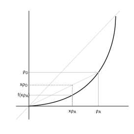
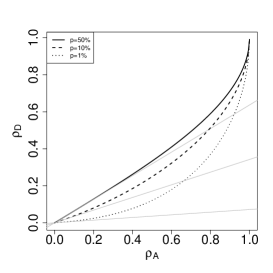
Figure 1: (a) Plot of the mapping function $f(\rho_{A})$ vs. $\rho_{A}$, which shows the relation between the asset correlation $\rho_{A}$ and the default correlation $\rho_{D}$. $f(\rho_{A})$ is downward convex and $f(x\rho_{A})\leq xf(\rho_{A})$ for $0\leq x\leq 1$. (b) We set $p=0.5$(solid), $0.1$(broken) and $0.01$(dotted). The gray lines show the lines with a slope of $A$ in Eq.(6). (c) Plot of $A$ vs. $p$.

We plot the mapping function $\rho_{D}=f(\rho_{A})$ in the $(\rho_{A},\rho_{D})$-plane in Fig. 1 under the conditions $f(0)=0$ and $f(1)=1$. The straight lines $\rho_{D}=A\rho_{A}$ with $A$ from Eq.(6) are plotted in Fig. 1 (b). We confirm that $A$ in Eq.(6) is the same as the slope of the tangent line at point $(\rho_{A},\rho_{D})=(0,0)$. We plot the relation between $p$ and $A$ in Fig. 1(c). From the convexity of $f(\rho_{A})$ in Fig. 1(a), we find the following inequality:

$$A\rho_{A}d_{i}<f(\rho_{A}d_{i})<f(\rho_{A})d_{i}=\rho_{D}d_{i}\,\,,\,\,\mbox{for}\,\,\,\,\rho_{A},\rho_{D}>0,0<d_{i}<1$$

Using this inequality, we form the upper bound for $V(Z(T))$ as:

$$\mbox{V}(Z(T)) = p(1-p)\frac{1}{nT}+p(1-p)\frac{(n-1)}{nT}f(\rho_{A})+2p(1-p)\frac{1}{T^{2}}\sum_{i=1}^{T-1}f(\rho_{A}d_{i})(T-i)$$

$$\leq p(1-p)\frac{1}{nT}+p(1-p)\frac{(n-1)}{nT}f(\rho_{A})+2p(1-p)\rho_{D}\frac{1}{T^{2}}\sum_{i=1}^{T-1}d_{i}(T-i).$$

The lower bound is then

$$V(Z(T))\geq p(1-p)\frac{1}{nT}+p(1-p)\frac{(n-1)}{nT}f(\rho_{A})+2p(1-p)A\rho_{A}\frac{1}{T^{2}}\sum_{i=1}^{T-1}d_{i}(T-i).$$

In both the upper and lower bounds, their third term is proportional to $\frac{1}{T^{2}}\sum_{i=1}^{T-1}d_{i}(T-i)$. Thus, we can estimate the asymptotic behavior of $V(Z(T))$ by the following expression:

$$\mbox{V}(Z(T))=p(1-p)\frac{1}{nT}+p(1-p)\frac{(n-1)}{nT}\rho_{D}+2p(1-p)c\frac{1}{T^{2}}\sum_{i=1}^{T-1}d_{i}(T-i),$$ (7)

where $c$ is a positive constant and $\rho_{D}>c>A\rho_{A}$.

II.1 2.1 Exponential temporal correlation

In this subsection, we study the convergence of $Z(T)$ for the exponential decay model $d_{i}=\theta^{i},\theta\leq 1$:

$$V(Z(T))\simeq p(1-p)\frac{1}{nT}+p(1-p)\frac{(n-1)}{nT}f(\rho_{A})+2p(1-p)c\frac{1}{T^{2}}\sum_{i=1}^{T-1}\theta^{i}(T-i).$$

The first two terms on the right-hand side (RHS) behave as $\propto 1/T$ and, thus, converge to 0 in the limit $T\to\infty$. In the case that $\theta\neq 1$, the third term is

$$2p(1-p)c\frac{1}{T^{2}}[T\frac{1-\theta^{T-1}}{1-\theta}+\frac{(T-1)\theta^{T-1}(1-\theta)-(1-\theta^{T-1})\theta}{(1-\theta)^{2}}\propto 1/T$$

and it converges to 0 in the limit $T\to\infty$. In addition, $C(t)\simeq A\rho_{A}\theta^{t}$ for large $t$. We conclude that as the number of data samples increases, the distribution of $Z(T)$ converges to a delta function and therefore, PD can be estimated empirically.

Thus, we calculate $C(t))=f(\rho_{A}\theta^{t})$ and $V(Z(t))$ numerically for $t\leq 10^{5}$. We set $\rho_{A}=0.5,n=10^{4},p=0.5,0.1,0.01$ and $\theta=0.8,0.9,0.99,0.999$. Figure 2 (a)-(c) shows the double logarithmic plot of $C(t)$ vs. $t$. Here, it is clearly seen that $C(t)$ decays exponentially. Figure 2 (d)-(f) shows the plot of V$(Z(t))$ vs. $t$. For all $\theta<1\in\{0.8,0.9,0.99,0.999\}$, $V(Z(t))$ decays as $1/t$. When $\theta=1$, there is no temporal correlation decay case and all obligors are correlated $\rho_{A}$. Hence, there is no phase transition for $\theta<1$.

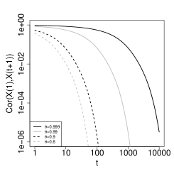
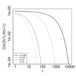
(a)	(b)	(c)
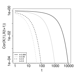
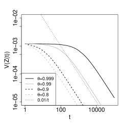
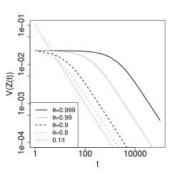
(d)	(e)	(f)

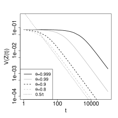
Figure 2: Plots of (a),(b),(c) $C(t)$ and (d), (e), (f) $V(Z(t))$ vs. $t$, for $\theta\in\{0.8,0.9,0.99,0.999\}$, Exponential decay case. The PDs are $1\%$ for (a) and (d), $10\%$ for (b) and (e), and $50\%$ for (c) and (f).

II.2 2.2 Power temporal correlation

In this subsection, we consider the power decay case $d_{i}=1/(i+1)^{\gamma},i=1,2,\cdots$, where $\gamma\geq 0$ is the power index. The power correlation affects the number of defaults for long periods of time. The ranges $\gamma\leq 1$ and $\gamma>1$ are called long memory and intermediate memory, respectively Long . On the other hand, the exponential decay affects short periods of time and it is called short memory. The asymptotic behavior of $V(Z(T))$ is given as:

$$\mbox{V}(Z(T))\simeq p(1-p)\frac{1}{nT}+p(1-p)\frac{(n-1)}{nT}f(\rho_{A})+2p(1-p)c\frac{1}{T^{2}}\sum_{i=1}^{T-1}(i+1)^{-\gamma}(T-i).$$

II.2.1 2.2.1) $\gamma>1$ case

We can obtain

$$V(Z(T)) \simeq \frac{p(1-p)}{nT}+\frac{p(1-p)(n-1)f(\rho_{A})}{nT}+\frac{2p(1-p)c}{T^{2}}\sum_{i=1}^{T-1}(T-i)/(i+1)^{\gamma}$$ (8)

$$\simeq \frac{p(1-p)}{nT}+\frac{p(1-p)(n-1)\rho_{D}}{nT}+2pqcT^{-\gamma}/(\gamma-1).$$

The first two terms decrease as $1/T$ and the third term decreases as $1/T^{\gamma}$ where $\gamma>1$. Hence, the significant terms are the first two terms and the convergence of $V(Z(T))$ behaves as $\sim 1/T$. The convergence speed is the same as that of the independent binomial case.

II.2.2 2.2.2) $\gamma=1$ case

$V(Z(T))$ behaves as

$$V(Z(T))\simeq\frac{p(1-p)}{nT}+\frac{p(1-p)(n-1)f(\rho_{A})}{nT}+\frac{2p(1-p)c}{T^{2}}\sum_{i=1}^{T-1}(T-i)/(i+1).$$ (9)

The RHS of Eq.(9) is evaluated as

$$RHS\simeq\frac{p(1-p)}{nT}+\frac{p(1-p)(n-1)f(\rho_{A})}{nT}+2p(1-p)c[(T+1)\log T-T+2]\sim\log T/T.$$ (10)

In conclusion, $V(Z(T))$ behaves asymptotically as

$$V(Z(T))\sim\log T/T$$ (11)

and the estimator $Z(T)$ converges to $p$ more slowly than in the normal case.

II.2.3 2.2.3) $\gamma<1$ case

$V(Z(T))$ is calculated as:

$$V(Z(T))\simeq\frac{p(1-p)}{nT}+\frac{p(1-p)(n-1)f(\rho_{A})}{nT}+2p(1-p)c[\frac{1}{(1-\gamma)(2-\gamma)T^{\gamma}}]\sim T^{-\gamma}.$$ (12)

Then, we can conclude $V(Z(T))$ behaves as

$$V(Z(T))\sim T^{-\gamma}.$$ (13)

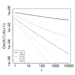
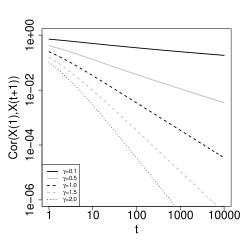
(a)	(b)	(c)
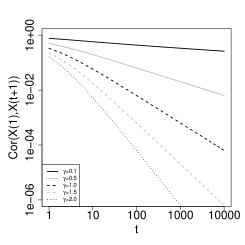
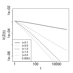
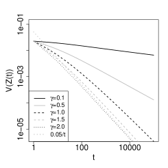
(d)	(e)	(f)

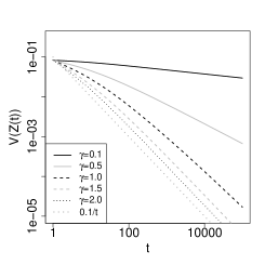
Figure 3: Plots of (a),(b),(c) $C(t)$ and (d),(e),(f) $V(Z(t))$ vs. $t$, for $\gamma\in\{3.0,2.0,1.5,1.0,0.5,0.1\}$. Power decay case. The PDs are $1\%$ for (a) and (d), $10\%$ for (b) and (e), and $50\%$ for (c) and (f).

In conclusion, a phase transition occurs when the temporal correlation decays by power law. When the power index, $\gamma$, is less than one, the PD estimator $Z(T)$ slowly converges to $p$. Conversely, when the power index $\gamma$ is greater than one, the convergence behavior is the same as that of the binomial distribution. This phase transition is called a ”super-normal transition” Hod ; Hisakado2 , which is the transition between long memory and intermediate memory. This transition is different from the phase transition found when we used the beta-binomial distribution in our previous work. In that article, when the power index was less than one, the PD estimator $Z(T)$ did not converge to $p$ when the beta-binomial model was used Hisakado6 .

Figure 4: Plots of $\log_{2}(Z(T)/Z(2T))$ with $T=10^{5}$ vs. $\gamma$. The PDs are $1\%$(dotted), $10\%$(broken) and $50\%$(solid).

To confirm the phase transition, we calculate $C(t)=f(\rho_{A}(t+1)^{-\gamma})$ and $V(Z(T))$. Fig. 3 (a)-(c) shows the double logarithmic plot of $C(t)$ vs. $t$. $C(t)$ decays by power law for $\gamma\in\{0.1,0.5,1.0,1.5,2.0\}$. For small $\gamma$, such as $0.5,0.1$, the slope is extremely small. Fig. 3 (d)-(f) shows the double logarithmic plot of $V(Z(t))$ vs. $t$. For $\gamma\in\{0.1,0.5,1.0,1.5,2.0\}$, $V(Z(t))$ decays as $1/t$. At $\gamma\leq 1$, the slope of the decay becomes less than one. In this case, the convergence becomes slower than in the normal case.

Next, we confirm the phase transition using finite size scaling. We estimate the exponent of the convergence of $Z(T)$. If we assume that $V(Z(T))\propto T^{-\delta}$, the exponent $\delta$ is estimated as

$$\delta=\log_{2}\frac{V(Z(T))}{V(Z(2T))}.$$

In the case $V(Z(T))\sim\ln T/T$, we have

$$\log_{2}\frac{V(Z(T))}{V(Z(2T))}=1-\log_{2}(1+\frac{2}{\ln T})<1.$$

We estimate $\delta$ numerically for $T=10^{5}$. We plot the results in Fig. 4. We see that $\delta=1$ for $\gamma>1$ and $\delta=\gamma$ for $\gamma<1$. When $\gamma\simeq 1$, the relation becomes obscured by the finite size effect.

In summary, when $\gamma>1$, $Z(T)$ converges to $p$ as in the normal case. On the other hand, when $\gamma\leq 1$, the convergence is slower than that of the normal case. Hence, there is the phase transition at $\gamma=1$.

III 3. Estimation of parameters

As discussed in the previous section, whether temporal correlation obeys an exponential decay or a power decay is an important issue because there exists a super-normal transition in the latter case. Further, the appearance of a transition affects whether we can estimate the PD.

First, the S&P default data from 1981 to 2018 Data1 are used. The average PD is 1.51 $\%$ for all ratings, 3.90 $\%$ for speculative grade (SG) ratings, and 0.09$\%$ for investment grade (IG) ratings. The SG rating represents ratings under BBB-(Baa3) and IG represents that above BBB-(Baa3). In Fig. 5 (a) we show the historical default rate of the S&P. The solid and dotted lines correspond to the speculative grade and investment grade samples, respectively. We use Moody’s default data from 1920 to 2018 for 99 years Data2 . It includes the Great Depression in 1929 and Great Recession in 2008. The average default rate is 1.50$\%$ for all of the ratings, $3.70\%$ for speculative ratings, and $0.14\%$ for investment grade. In Fig. 5 (b), we show the historical default rate of Moody’s.

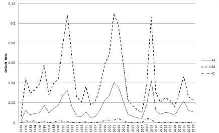
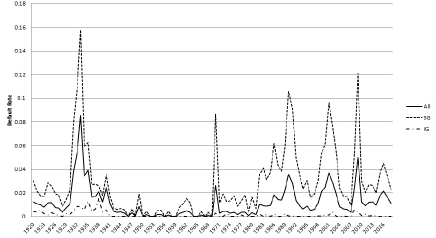
(a) (b)

Figure 5: (a): S&P Default Rate in 1981-2018. (b)Moody’s Default Rate in 1920-2018. The solid and dotted lines respectively correspond to the speculative grade (SG) and investment grade (IG) of all the samples.

Table 1: MAP estimation of the parameters for the exponential and power decay models by the Merton model

			Exponential decay			Power decay
No.	Model	$p$	$\rho_{D}$	$\theta$	$p$	$\rho_{D}$	$\gamma$
1	Moody’s 1920-2018	1.43%	17.8%	0.858	7.40%	38.7%	0.090
2	S&P 1981-2018	1.43%	6.4%	0.597	1.85%	12.0%	0.610
3	Moody’s 1981- 2018	1.61%	7.1%	0.613	1.92%	12.4%	0.622
4	S&P 1990-2018	1.72%	7.5%	0.616	2.97%	12.5%	0.616
5	Moody’s 1990-2018	1.92%	10.0%	0.678	2.40%	12.1%	0.624
6	Moody’s 1920-2018 SG	3.00%	18.9%	0.838	6.15%	32.2%	0.146
7	S&P 1981-2018 SG	4.53%	8.7%	0.588	4.42%	11.7%	0.628
8	Moody’s 1981-2018 SG	4.28%	9.4%	0.603	3.97%	11.5%	0.619
9	S&P 1990-2018 SG	4.93%	11.2%	0.639	5.40%	13.9%	0.626
10	Moody’s 1990-2018 SG	4.51%	11.1%	0.648	6.09%	14.6%	0.619
11	Moody’s 1920-2018 IG	0.04%	35.3%	0.891	3.40%	51.4%	0.102
12	S&P 1981-2018 IG	0.02%	25.8%	0.483	0.02%	20.3%	9.189
13	Moody’s 1981-2018 IG	0.01%	21.9%	0.672	1.84%	33.8%	0.618
14	S&P 1990-2018 IG	0.01%	37.4%	0.712	1.63%	46.7%	0.630
15	Moody’s 1990-2018 IG	0.01%	33.0%	0.794	3.44%	51.1%	0.003

We estimate the parameters $p,\rho_{A},\theta$ and $\gamma$ of the Merton model using the Bayesian method and Stan 2.19.2 in R 3.6.2 software. We explain the method and how to estimate the parameters in Appendix B Tas2 and summarize the results in Table 1. We show $\rho_{D}$ instead of $\rho_{A}$, as we need to compare it with that of the beta-binomial distribution model. The estimation of the parameters are the maximum a posteriori (MAP) estimation. A detailed explanation of the estimation procedure and rmd file is provided on github git . We notice that the power index $\gamma$ is smaller than 1 for all cases and the values are smaller than the phase transition point, $\gamma=1$.

We compare these results to the MAP estimation using the beta-binomial distribution by using the same data Hisakado6 . The conclusions are shown in Table 2 for the exponential and power decay models. We confirmed small $\theta$ and large $\gamma$ values, which represent small temporal correlation. The parameter $\gamma$ for the power decay is larger than the phase transition point, $\gamma=1$. The PD and default correlation are almost the same as the estimations by the exponential and power decay models. The reason behind this is that the power exponent $\gamma$ is adequately large and there is only a small difference between the exponential and power decay models.

Table 2: Most likelihood estimate of the parameters for the exponential and power decay models by beta-binomial distribution

			Exponential decay			Power decay
No.	Model	$p$	$\rho_{D}$	$\theta$	$p$	$\rho_{D}$	$\gamma$
1	Moody’s 1920-2018	0.96%	1.9%	0.044	0.94%	2.0%	4.7
2	S&P 1981- 2018	1.53%	0.8%	0.026	1.54%	0.8%	5.7
3	Moody’s 1981-2018	1.53%	0.8%	0.022	1.52%	0.7%	5.9
4	S&P 1990-2018	1.66%	0.9%	0.023	1.64%	0.9%	5.7
5	Moody’s 1990-2018	1.67%	0.9%	0.019	1.61%	0.8%	6.0
6	Moody’s 1920-2018 SG	2.36%	3.8%	0.044	2.34%	4.1%	4.7
7	S&P 1981-2018 SG	4.16%	2.0%	0.026	4.20%	2.0%	5.7
8	Moody’s 1981-2018 SG	4.18%	2.0%	0.022	4.35%	1.9%	6.0
9	S&P 1990-2018 SG	4.42%	2.5%	0.024	4.43%	2.6%	5.6
10	Moody’s 1990-2018 SG	4.33%	2.3%	0.020	4.31%	2.2%	5.9
11	Moody’s 1920-2018 IG	0.13%	0.8%	0.17	0.11%	0.9%	3.0
12	S&P 1981-2018 IG	0.11%	0.4%	0.12	0.09%	0.3%	3.6
13	Moody’s 1981-2018 IG	0.10%	0.6%	0.05	0.09%	0.3%	4.6
14	S&P 1990-2018 IG	0.09%	0.4%	0.12	0.09%	0.4%	3.7
15	Moody’s 1990-2018 IG	0.09%	0.4%	0.06	0.07%	0.7%	4.2

We can confirm that $\theta$ and $\gamma$ both have large differences between the values estimated by the beta-binomial distribution and the Merton model. The reason for this is shown in Fig. 1 (a). We set $d_{1A}$ and $d_{1D}$ for $\rho_{A}$ and $\rho_{D}$, respectively. From this, we can obtain the inequality

$$d_{1A}=\frac{d_{1A}\rho_{A}}{\rho_{A}}>>\frac{f(d_{1A}\rho_{A})}{f(\rho_{A})}=\frac{f(d_{1A}\rho_{A})}{\rho_{D}}=d_{1D}.$$

Hence, the difference in the estimated parameter between the Merton model and the beta-binomial model becomes large. We can find the large convexity for the mapping function $f$. Hence, $\theta$ and $\gamma$ for a default correlation is much smaller than that for asset correlation.

Next, we discuss whether the correlation has a long memory. In Table 3, we calculated the WAIC and WBIC for each model that uses the Merton model for the discussion. Using Moody’s data from 1920, the power decay model is found to be superior to the exponential decay model. Therefore, it seems that the default rate has a long memory. As $\gamma$ is less than 1 for long history data, the phase is in the slow convergence phase. In other words, parameter estimation becomes difficult because the convergence speed becomes slow when the temporal correlation is the power decay.

In Table 4, we show the AIC and BIC for each model using the beta-binomial distribution and compare them to the estimation using Merton model. We obtain the same conclusion using Moody’s data from 1920: the power decay model is superior to the exponential decay model. The parameter $\gamma$ is not less than 1 for power decay case when we use the beta-binomial distribution.

Table 3: WAIC and WBIC for the exponential and power decay using the Merton model

		Exponential decay		Power decay
No.	Model	WAIC	WBIC	WAIC	WBIC
1	Moody’s 1920-2018	572.9	746.7	568.6	745.9
2	S&P 1981- 2018	271.5	332.9	272.1	334.8
3	Moody’s 1981-2018	277.6	339.0	277.5	341.4
4	S& P 1990-2018	214.3	256.4	214.6	258.3
5	Moody’s 1990-2018	219.5	262.1	219.6	264.7
6	Moody’s 1920-2018 SG	564.3	731.9	560.2	733.8
7	S&P 1981-2018 SG	268.7	328.1	268.9	330.5
8	Moody’s 1981-2018 SG	274.1	333.6	274.4	337.1
9	S& P 1990-2018 SG	212.0	253.9	212.8	255.2
10	Moody’s 1990-2018 SG	217.3	260.4	218.3	262.8
11	Moody’s 1920-2018 IG	247.6	351.2	244.9	351.2
12	S&P 1981-2018 IG	116.0	153.3	115.0	160.3
13	Moody’s 1981-2018 IG	110.3	156.3	108.8	156.7
14	S&P 1990-2018 IG	87.6	114.3	86.8	117.7
15	Moody’s 1990-2018 IG	81.7	111.4	82.5	114.5

Table 4: AIC and BIC for the exponential and power decay using the beta-binomial distribution

		Exponential decay		Power decay
No.	Model	AIC	BIC	AIC	BIC
1	Moody’s 1920-2018	746.8	780.8	746.8	780.9
2	S&P 1981- 2018	352.0	382.9	353.6	384.5
3	Moody’s 1981-2018	362.2	395.0	363.4	396.2
4	S& P 1990-2018	285.0	315.5	285.8	316.3
5	Moody’s 1990-2018	293.8	326.3	298.6	331.1
6	Moody’s 1920-2018 SG	730.8	762.0	730.6	761.8
7	S&P 1981-2018 SG	346.8	366.7	348.8	368.7
8	Moody’s 1981-2018 SG	356.0	385.9	360.4	390.3
9	S& P 1990-2018 SG	283.0	302.6	283.8	303.4
10	Moody’s 1990-2018 SG	291.0	320.7	291.6	321.3
11	Moody’s 1920-2018 IG	302.2	334.9	300.4	333.1
12	S&P 1981-2018 IG	134.9	164.5	136.1	165.7
13	Moody’s 1981-2018 IG	142.3	173.7	140.2	171.7
14	S&P 1990-2018 IG	106.0	135.3	107.2	136.5
15	Moody’s 1990-2018 IG	111.8	142.8	112.4	143.4

IV 4. Concluding Remarks

In this study, we introduced the Merton model with temporal asset correlation and discussed the convergence of the estimator of the probability of default. We adopted a Bayesian estimation method to estimate the model’s parameters and discussed its implication in the estimation of PD. We found a phase transition when the temporal correlation decayed by a power curve, which meant that the correlation had a long memory. When the power index $\gamma$ was larger than one, the estimator distribution of the PD converged normally. When the power index was less than or equal to 1, the distribution converged slowly. This phase transition is called the ”super-normal transition”. For the case of an exponential decay, there was no phase transition.

In our previous work, we studied a beta-binomial distribution model with temporal default correlation. The estimator of PD also showed a phase transition in the power decay case. The transition depended on whether the distribution converged or not. It was different from the phase transition found in the present study.

The main difference between the Merton model and the beta-binomial distribution model is the incorporation of default correlation. In the latter model, the default correlation is defined by binary variables. In the former, the default correlation is incorporated into the asset correlation, which is defined by a continuous variable. The implication of the present study is about the difficulty in the estimation of PD when we adopt the former models. The estimated power index is in the slow convergence region of PD. Even with empirical data over a long period of time, PD is difficult to estimate when we adopt the proposed model.

Appendix A Appendix A. Temporal correlation for the Merton Model

We consider the assets of two obligors, $\hat{U}_{1t}$ and $\hat{U}_{2t}$, in year $t$ to confirm temporal correlation. The assets of two obligors have the correlation $\rho_{A}$. $S_{t}$ is the global economic factor that affects the two obligors at $t$:

$$\hat{U}_{1t} = \sqrt{\rho_{A}}S_{t}+\sqrt{1-\rho_{A}}\epsilon_{1t},$$

$$\hat{U}_{2t} = \sqrt{\rho_{A}}S_{t}+\sqrt{1-\rho_{A}}\epsilon_{2t},$$ (14)

where $\epsilon_{1}$ and $\epsilon_{2}$ are the individual factors for the obligors. Here, there is no correlation among $\epsilon_{1}$, $\epsilon_{2}$, and $S_{t}$ because they are independent of each other. In the following year, $t+1$, the assets of the two obligors are $\hat{U}_{1t+1}$ and $\hat{U}_{2t+1}$. The assets have the same correlation, $\rho_{A}$, through the global factor $S_{t+1}$. We can write this as:

$$\hat{U}_{1t+1} = \sqrt{\rho_{A}}S_{t+1}+\sqrt{1-\rho_{A}}\epsilon_{1t+1},$$

$$\hat{U}_{2t+1} = \sqrt{\rho_{A}}S_{t+1}+\sqrt{1-\rho_{A}}\epsilon_{2t+1}.$$ (15)

The temporal correlation between $t$ and $t+1$ is $d_{1}$. The correlation between $\hat{U}_{1t}$ and $\hat{U}_{2t+1}$ is $d_{1}\rho_{A}$. In the same way, we obtain the temporal correlation matrix, Eq.(5). It is same as that from the Bayesian estimation, which was introduced in Hisakado6 , without differentiating between the asset and default correlations.

Appendix B Appendix B. Bayesian estimation using the Merton model

In this Appendix we explain the estimate of parameters using the Merton model Tas2 . There is a prior belief of the possible value on the PD. The prior belief is updated by observations while using the prior distribution as a weighting function. Here, we use the prior function, which is a uniform prior distribution.

To calculate the unconditional probability $P(X_{1}=k_{1},\cdots,X_{T}=k_{T})$, we approximate the solution by Monte Carlo simulations and numerical integration. Here, the number of obligors and defaults in the $t$-th year are $n_{t}$ and $k_{t}$, respectively, and they are observable variables. The likelihood is

$$P(X_{1}=k_{1},\cdots,X_{T}=k_{T})\sim\sum_{i=1}^{n}\prod_{t=1}^{T}\frac{n_{t}!}{k_{t}!(n_{t}-k_{t})!}G(S_{t}^{i})^{k_{t}}(1-G(S_{t}^{i}))^{(n_{t}-k_{t})},$$ (16)

where $G(S_{t}^{i})$ is defined as the probability that an obligor will default in year $t$, which is conditional to the　$i$-th path realization of all global factors such that

$$G(S_{t}^{i})=\Phi(\frac{\Phi^{-1}(p)-S_{t}^{i}\sqrt{\rho_{A}}}{\sqrt{1-\rho_{A}}}),$$ (17)

where $\rho_{A}$ is the asset correlation among obligors within a one year window and $\Phi$ is the cumulative normal distribution. $S_{t}^{i}$ is the correlated multi-dimensional normal distribution and we use the MAP estimation to estimate the parameters.

We have estimated parameters using a beta-binomial distribution provided in Section 3 and Hisakado6 . One of the differences between using the Merton model and beta-binomial distribution is the default correlation and the asset correlation. The default correlation is defined by binary variables. On the other hand, the asset correlation is defined by continuous variables. The other difference is that one can calculate the parameters analytically when using the beta-binomial distribution. Hence, it is easier to estimate parameters when using the beta-binomial distribution than when using the Merton model. In fact, we estimate the parameters to be stable in Section 3, especially for IG samples, which have small PD. The estimation of IG samples using the Merton model is difficult.

References

- (1) G. Galam, Stat. Phys. 61, 943 (1990).
- (2) G. Galam, Inter J. Mod. Phys. C 19(03), 409 (2008).
- (3) N. M. Mantegna and H. E. Stanley, Introduction to Econophysics: Correlations and Complexity in Finance (Cambridge University Press, 2000).
- (4) D. Brockmann, L. Hufinage, and T. Geisel, Nature 439, 462 (2006).
- (5) I. T. Wong, M. L. Gardel, D. R. Reichman, E. R. Weeks, M. T. Valentine, A. R. Bausch, and D. A. Weitz, Phys. Rev. Lett. 92, 178101 (2004).
- (6) Y. Gefen, A. Aharony, and S. Alexander, Phys. Rev. Lett. 50, 77 (1983).
- (7) R. Metzler and J. Klafter, Phys. Rep. 339, 1 (2000).
- (8) S. Hod and U. Keshet, Phys. Rev. E 70 11006 (2004).
- (9) T. Huillet, J. Phys. A 41 505005 (2008).
- (10) G.Schütz and S. Trimper, Phys. Rev. E 70 045101 (2004)
- (11) S Mori. and M. Hisakado., J. Phys. Soc. Jpn. 79, 034001 (2010).
- (12) M. Hisakado and S. Mori, J. Phys. A 43, 31527 (2010).
- (13) M. Hisakado and S. Mori, J. Phys. A 44, 275204 (2011).
- (14) M. Hisakado and S. Mori, J. Phys. A 45, 345002 (2012).
- (15) M. Hisakado and S. Mori, Physica A 417, 63 (2015).
- (16) M. Hisakado and S. Mori, Physica. A. 108, 570 (2016).
- (17) M. Hisakado and S. Mori, Physica A, 123480 (2019)
- (18) S. Hod and U. Keshet, Phys. Rev. E 70, 11006 (2004).
- (19) S. Mori, K. Kitsukawa, and M. Hisakado, Quant. Fin.10, 1469 (2010).
- (20) S. Mori, K. Kitsukawa, and M. Hisakado, J. Phys. Sco.Jpn. 77, 114802 (2008).
- (21) P. J. Schönbucher, Cresit Derivatives Pricing Models:Models, Pricing, and Inplementation (John Wiley & Sons, Ltd. 2003).
- (22) K. Pluto and D. Tasche, Estimating Probabilities of Default for Low Default Portfolios In: Engelmann. B., Rauhmeier R. (eds) The Basel II Risk Parameters. Springer, Berlin, Heidelberg (2011).
- (23) N. Benjamin, A. Cathcart, and K. Ryan K,Low Default Portfolios: A Proposal for Conservative Estimation of Default Probabilities (Financial Services Authority, 2006).
- (24) O. Vasicek, Risk 15(12), (2002) 160
- (25) R. C. Merton, J. Fin. 29(2), 449 (1974).
- (26) I. Florescu, M. C. Mariani, H. E. Stanley, and F. G. Viens (Eds.) Handbook of High-Frequency Trading and Modeling in Finance John Wiley& Sons (2016)
- (27) 2018 Annual Global Corporate Default Study and Rating Transitions (S& P Global Ratings, 2019).
- (28) Moody’s Annual Default Study: Corporate default and recovery dates, 1920-2018 (Moody’s 2019).
- (29) D. Tasche, J. Risk Management in Financial Institutions, 6(3) 302-326 (2013).
- (30) https://github.com/shintaromori/DefaultCorrelation.