Controlled self-similar matter waves in PT-symmetric waveguide

Abstract

We study the dynamics of Bose-Einstein condensate coupled to a waveguide with parity-time symmetric potential in the presence of quadratic-cubic nonlinearity modelled by Gross-Pitaevskii equation with external source. We employ the self-similar technique to obtain matter wave solutions, such as bright, kink-type, rational dark and Lorentzian-type self-similar waves for this model. The dynamical behavior of self-similar matter waves can be controlled through variation of trapping potential, external source and nature of nonlinearities present in the system.

1 Introduction

Bose-Einstein condensate (BEC) is a macroscopic quantum state of matter in which all atoms in the bosonic gas condenses into a single ground state of the system [1, 2]. The coherent matter-wave formed via this population of atoms is depicted by a macroscopic wave function which is also a solution of nonlinear Schrödinger equation (NLSE). The mean-field equation used to describe the dynamics of BEC is the Gross-Pitaevskii (GP) equation or NLSE with a trapping potential [3]. Basically, the GP equation is a three-dimensional equation which can be reduced to a one- or two-dimensional equation by confining the condensate to two or one directions in an effective potential [4, 5]. In BECs, the formation of soliton solutions is resultant of the interactions among atoms and the geometry of the trap used to confine the BEC. Here, nonlinearity arises due to interatomic interactions of the condensate measured by the scattering length ‘$a$’. In BEC, Feshbach resonance gives a way to control the strength of how atoms interact with each other [6]. Experimental work has been done to show the existence of bright solitons for attractive interactions ($a<0$) [7] and dark solitons for repulsive interactions ($a>0$) [8]. Authors have also studied the dynamics of BEC in the presence of competing cubic-quintic nonlinearity [9, 10, 11, 12, 13, 14, 15] and quadratic-cubic nonlinearity [16, 17, 18, 19, 20]. Over the past several years, there is a considerable interest on the existence of matter wave solutions for GP equation with time-dependent coefficients or generalized nonlinear Schrödinger equation (GNLSE) [21, 22, 23, 24, 25]. Earlier, Paul and his collaborators [26, 27, 28] numerically studied the resonant transport of interacting BEC through a symmetric double barrier potential in a waveguide for the modified GP equation. Coupling of the waveguide to a reservoir of condensate from which matter waves are injected into the guide is modelled by source term. Later, Yan et al. [29] studied the nonautonomous matter waves in a waveguide for the modified GP equation driven by a source term. Recently, R. Pal et al. [20] obtained the matter wave self-similar solutions for the driven nonautonomous GP equation with quadratic-cubic nonlinearity. Apart from it, the GNLSE with external source has also been studied to obtain self-similar solution in the context of fiber optics [30, 31, 32].

In this work, we have studied the dynamics of BEC coupled to a waveguide with parity-time (PT) symmetric potential modelled by GP equation with inhomogeneous source, $S(t)e^{i\theta(x,t)}$ where $S(t)$ and $\theta(x,t)$ are amplitude and phase terms [27, 29]. The source term simulates the coherent injection of matter waves from an external reservoir to the waveguide. In recent years, a significant work has been done on the evolution of soliton [33, 34, 35, 36] and self-similar solutions [37, 38, 39] for the GNLSE with PT-symmetric potential. According to quantum mechanics, Hamiltonian of a system should be Hermitian since the eigenvalues corresponding to Hermitian operators are always real. In 1998, Carl Bender and S. Boettecher [40] proposed that even non-Hermitian Hamiltonians exhibit real spectra provided Hamiltonians respect PT-symmetry. The necessary but not sufficient condition for Hamiltonian to be PT-symmetric is that the real and imaginary parts of the potential should be even and odd function w.r.t coordinates, respectively [41]. Initially, the idea of PT-symmetry was introduced in the field of quantum mechanics [40] and then this idea has found rapid applications in numerous other fields. In the field of optics, PT was implemented by Christodouldes and his collaborators [42, 43, 44] by choosing the complex potential as PT-symmetric such that the real part models the waveguide profile and imaginary part models gain/loss in the media. In refs. [45, 46, 47], authors have studied the nonlinear model for the dynamics of BEC in PT-symmetric potential. In the context of BEC arrays, work has been done to study the nonlinear excitations in the presence of uniform distribution of atomic population which refer to as uniform background [48]. The matter wave solutions with background is explored in different trap geometries and interactions [48, 49, 50, 51]. Motivated from the above works, we consider driven quadratic-cubic GP equation in the presence of PT-symmetric potential and report the existence of bright, kink, rational dark and Lorentzian-type self-similar matter wave solutions on uniform background for this model. Kink solitons (also known as domain walls) have been reported for two-component condensates with cubic nonlinearity [52, 53]. These domain walls represent a transient layer between semi-infinite domains carrying different components, or distinct combinations of the components. Later on, the kink solutions also obtained for single component condensates with cubic-quintic nonlinearity [54, 55]. In earlier works, our group has done a considerable work on the self-similar solutions for GNLSE and proposed an analytical approach to control the dynamics of these solutions [25, 56, 57]. Here, in this work, we control the dynamical behavior of self-similar matter waves by varying the trapping potential, nonlinearity coefficient and source profile.

The manuscript is organized as follows : In Section 2, we discuss about the model equation and self-similar technique. In section 3, we describe the self-similar matter wave solutions for different profiles of trapping potential. Section 4 summarizes the work.

2 Model equation

The dynamics of BEC coupled to a waveguide in the presence of quadratic-cubic nonlinearity modelled by modified GP equation with external source as

$$i\hslash\frac{\partial\psi}{\partial t}=\Bigg{(}-\frac{\hslash^{2}}{2m}\frac{\partial^{2}}{\partial x^{2}}+V(x,t)+g_{1D}(t)|\psi|^{2}+g_{2D}(t)|\psi|\Bigg{)}\psi+S(t)e^{i\theta(x,t)},$$ (1)

where $\psi$ is the macroscopic wave function, $t$ is the time and $x$ is the transverse direction. Eq. 1 appears as an approximate model that governs the evolution of the macroscopic wave function of a cigar-shaped one-dimensional BEC. Here, $g_{1D}(t)$ and $g_{2D}(t)$ are the cubic and quadratic nonlinearity coefficients, describes repulsive contact interactions between atoms carrying dipole moments [58] and dipole-dipole attraction [59]. The source term, $S(t)e^{i\theta(x,t)}$ with $S(t)$ and $\theta(x,t)$ as amplitude and phase, represents the coupling of BEC reservoir to a waveguide [27, 29]. $V(x,t)$ represents the complex potential, given as $V(x,t)=\frac{F(t)x^{2}}{2}+i\frac{H(t)}{2}$, where $\frac{F(t)x^{2}}{2}$ is time dependent parabolic trapping potential, and $H(t)$ is gain or loss term and account for the interaction of atomic and thermal cloud. The complex potential is PT-symmetric if the real and imaginary parts of the potential must be an even and odd functions along the longitudinal direction, respectively, i.e. $F(t)=F(-t)$ and $H(t)=-H(-t)$. In Ref. [60], authors have investigated the light propagation in optical waveguides satisying PT-symmetry along the longitudinal direction. Normalizing the time and length in Eq. (1) in units of ${\omega_{\perp}}^{-1}$ and $\sqrt{\frac{h}{m\omega_{\perp}}}$ where ${\omega_{\perp}}$ defines the transverse trapping frequency, the dimensionless form of GP equation with a source term can be expressed as

$$i\frac{\partial\psi}{\partial t}=-\frac{1}{2}\frac{\partial^{2}\psi}{\partial x^{2}}+f(t)\frac{x^{2}}{2}\psi+\frac{i}{2}h(t)\psi+g_{1}(t)|\psi|^{2}\psi+g_{2}(t)|\psi|\psi+s(t)e^{i\theta(x,t)}.$$ (2)

Eq. (2) is linked with $\frac{\delta\mathscr{L}}{\delta\psi^{*}}=0$ where Lagrangian density can be written as

$$\mathscr{L}=i(\psi\psi_{t}^{*}-\psi_{t}\psi^{*})+|\psi_{x}|^{2}+(f(t)x^{2}+ih(t))|\psi|^{2}+g_{1}(t)|\psi|^{4}+\frac{4}{3}g_{2}(t)|\psi|^{3}+2s(t)e^{i\theta(x,t)}\psi^{*},$$ (3)

where $\psi^{*}(x,t)$ indicates the complex conjugate of the wave function $\psi(x,t)$.

3 Self-similar matter waves

In order to obtain the matter wave solutions of Eq. (2), we choose self-similar transformation as [61, 62]

$$\psi(x,t)=A(t)~{}~{}U\left[\frac{x-x_{c}(t)}{W(t)},\zeta(t)\right]e^{i\phi(x,t)},$$ (4)

where $A(t)$, $W(t)$ and $x_{c}(t)$ are the dimensionless amplitude, width and center position of the self-similar wave, respectively. The phase is chosen as

$$\phi(x,t)=C_{1}(t)\frac{x^{2}}{2}+C_{2}(t)x+C_{3}(t),$$ (5)

where $C_{1}(t)$, $C_{2}(t)$ and $C_{3}(t)$ are the parameter related to the phase-front curvature, the frequency shift and the phase shift, respectively, to be determined. Substituting Eq. (4) and Eq. (5) into Eq. (2), one obtains the quadratic-cubic NLSE with drive as

$$i\frac{\partial U}{\partial\zeta}+\frac{1}{2}\frac{\partial^{2}U}{\partial\chi^{2}}+a_{1}|U|^{2}U+a_{2}|U|U=a_{3}~{}e^{i(\theta-\phi)},$$ (6)

where the amplitude, similarity variable, effective propagation distance, guiding-center position, cubic nonlinearity, quadratic nonlinearity, source term and phase are given as

$$A(t)=\frac{1}{W(t)},~{}~{}\chi(x,t)=\frac{x-x_{c}(t)}{W(t)},~{}~{}\zeta(t)=\zeta_{0}+\int_{0}^{t}\frac{ds}{W^{2}(s)},$$ (7)

$$x_{c}(t)=W(t)\Bigg{(}x_{0}+C_{02}\int_{0}^{t}\frac{ds}{W^{2}(s)}\Bigg{)},~{}~{}g_{1}=-a_{1},~{}~{}g_{2}=-a_{2}~{}A(t),$$ (8)

,

$$s(t)=a_{3}~{}A^{3}(t),~{}~{}\phi(x,t)=\frac{x^{2}}{2W}\frac{\partial W}{\partial t}+\frac{C_{02}x}{W}-\frac{C^{2}_{02}}{2}\int_{0}^{t}\frac{ds}{W^{2}(s)},$$ (9)

with $C_{2}(0)=C_{02}$, $x_{c}(0)=x_{0}$, $W(0)=1$, and $a_{1}$, $a_{2}$, $a_{3}$ are constants. Here, $a_{1}$ and $a_{2}$ are parameters for cubic and quadratic coefficient, respectively. The parameter $a_{3}$ modulate the source profile. For positive value of $a_{3}$, source has similar profile as amplitude ‘$A$’ and for negative values of $a_{3}$, profile is inverted which can be obtained by inserting a extra phase difference of ‘$\pi$’ between source and matter wave. The trapping potential and gain / loss are associated to self-similar wave width as

$$\frac{d^{2}W}{dt^{2}}-f(t)W=0,~{}~{}~{}h(t)=-\frac{d[lnW(t)]}{dt}.$$ (10)

As stated earlier, transformation given by Eq. (4) reduces Eq. (2) to the constant coefficient quadratic-cubic NLSE with external source given by Eq. (6). This equation is considered in the work of Pal et al. [19] to obtain a wide class of localized solutions under different parametric constraints. For all these localized solutions of Eq. (6), the corresponding self-similar matter wave solutions of Eq. (2) can be obtained by means of the reverse transformation variables and functions. In order to make the paper self-contained, we sketch the essential steps of Ref. [19]. We consider the following form of travelling wave solution for Eq. (6)

$$U(\chi,\zeta)=B(\xi)~{}~{}e^{i(k\chi-\omega\zeta)},$$ (11)

where $\xi=\alpha(\chi-v\zeta)$ is the travelling coordinate with $k$, $v$ and $\omega$ as wave parameters, and $\alpha$ is a constant. Substituting Eq. (11) into Eq. (6), assuming $\theta(x,t)=k\chi-\omega\zeta+\phi(x,t)$, and separating the real and imaginary parts, we obtain

$$v=k,$$ (12)

and

$$\frac{1}{2}\alpha^{2}B^{\prime\prime}+a_{1}B^{3}+a_{2}B^{2}+\sigma B=a_{3},$$ (13)

where $\sigma=\omega-\frac{1}{2}k^{2}$. Using a scaling transformation

$$B(\xi)=\rho(\xi)+\beta,$$ (14)

where $\beta$ is a scaling parameter, Eq. (13) reduces to

$$\frac{1}{2}\alpha^{2}\rho^{\prime\prime}+a_{1}\rho^{3}+\eta\rho^{2}+\epsilon\rho-\delta=0,$$ (15)

where $\eta=3a_{1}\beta+a_{2}$, $\epsilon=3a_{1}\beta^{2}+2a_{2}\beta+\sigma$, $\delta=-(a_{1}\beta^{3}+a_{2}\beta^{2}+\sigma\beta-a_{3})$. Here, $\eta$, $\epsilon$ and $\delta$ are effective quadratic coefficient, effective linear term and effective source coefficient. This reduction helps us to obtain a class of soliton solution by taking $\eta$, $\epsilon$ and $\delta$ equal to zero in Eq. (15) while the actual source, quadratic coefficient and linear term is non-zero in the Eq. (13). We studied the evolution of matter waves for two types of trapping potential for specific form of width profile as per Eq. (10), pertaining to the condition that complex potential should be PT-symmetric. Here, we have choosen sech-type and Gaussian-type profiles for trapping potential to study the dynamics of BEC.

3.1 Sech-type trapping potential

For $W(t)=a+\mbox{sech(t)}$, the trapping potential and gain / loss functions [refer Eq. (10)] takes the form,

$$f(t)=\frac{[-3+\text{cosh}(2t)]~{}\text{sech}^{3}(t)}{2~{}[a+\text{sech}(t)]},~{}~{}h(t)=\frac{\text{sech}(t)~{}\text{tanh}(t)}{a+\text{sech}(t)}.$$ (16)

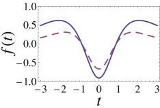
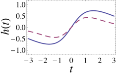
Figure 1: Profiles of trapping potential $f(t)$ for $a=0.1$ (solid line), $a=0.5$ (dotted line) and gain / loss function $h(t)$ for $a=0.1$ (solid line), $a=0.5$ (dotted line), respectively.

The profile of trapping potential and gain / loss functions is shown in Fig. (1) for different values of ‘$a$’. As value of ‘$a$’ increases, the magnitude of trapping potential decreases. From Fig. (1), one can observe that trapping potential ‘$f(t)$’ is an even-function whereas ‘$h(t)$’ is an odd-function of time variable, which is the necessary conditions for a complex potential to be PT-symmetric. Here, the free parameter ‘$a$’ should be non-zero, as $a=0$ leads to singularity in quadratic nonlinearity. Next, we will study the evolution of self-similar waves for this choice of trapping potential.

Bright and kink self-similar waves

For $\eta=0$ and $\delta=0$, Eq. (15) reduces to well known cubic elliptic equation which admits either bright or dark solitons depending upon the sign of cubic nonlinearity coefficient. These conditions put the constraint on various parameters as follows

$$\beta=\frac{-a_{2}}{3a_{1}},\epsilon=\sigma-\frac{a_{2}^{2}}{3a_{1}},\sigma=\frac{2a_{2}^{2}}{9a_{1}}-\frac{3a_{1}a_{3}}{a_{2}}.$$ (17)

For $a_{1}>0$ and $\epsilon<0$ which implies $\sigma<\frac{a_{2}^{2}}{3a_{1}}$, the cubic elliptic equation possesses bright soliton expressed as [63]

$$\rho(x,t)=\sqrt{\frac{-2\epsilon}{a_{1}}}\mbox{sech}\Bigg{(}\sqrt{\frac{-2\epsilon}{\alpha^{2}}}\xi\Bigg{)}.$$ (18)

The condition $\sigma=\frac{2a_{2}^{2}}{9a_{1}}-\frac{3a_{1}a_{3}}{a_{2}}$ fixes the source term as $a_{3}>\frac{-a_{2}^{3}}{27a_{1}^{2}}$ or $a_{3}<\frac{-a_{2}^{3}}{27a_{1}^{2}}$ for $a_{2}$ to be positive or negative, respectively. It implies that the model possesses bright self-similar waves for both cases such as cubic and quadratic nonlinearities are of same or competitive nature depending upon the sign of $a_{1}$ and $a_{2}$ to be same or opposite. Using Eq. (18) along with Eqs. (14) and (11) into Eq. (4), the complex wave solution for Eq. (2) can be written as

$$\psi(x,t)=\frac{1}{W(t)}\Bigg{[}\sqrt{\frac{-2\epsilon}{a_{1}}}\mbox{sech}\Bigg{(}\sqrt{\frac{-2\epsilon}{\alpha^{2}}}\xi\Bigg{)}-\frac{a_{2}}{3a_{1}}\Bigg{]}~{}e^{i(k\chi-\omega\zeta+\phi(x,t))}.$$ (19)

We have depicted the Intensity distribution, $|\psi(x,t)|^{2}$, of bright self-similar waves in Fig. (2) for competitive nonlinearities and different values of ‘$a$’ as $a=0.1$ and $a=0.5$, respectively. The nonlinearity coefficients are chosen as $a_{1}=0.8$, $a_{2}=-1.2$ and source coefficient as $a_{3}=0.09$. The other parameters used are $v=1$, $\alpha=1$, $\zeta_{0}=0$, $x_{0}=0$ and $C_{02}=0.3$. From plot, one can observe that for small values of ‘$a$’, that is large amplitude of trapping potential as shown in Fig. (1), the intensity of bright self-similar matter wave is more. Hence, the self-similar waves gets more intensive and compressive as value of ‘$a$’ decreases. Thus one can amplify the propagating wave by judicious choice of parameter ‘$a$’. Further, we have plotted the intensity profile of bright self-similar matter wave in Fig. (3) to analyze the effect of same sign of nonlinearities and negative magnitude of source coefficient. For same sign of nonlinearities chosen as $a_{1}=0.8$ and $a_{2}=1.2$, we observe W-shaped self-similar waves [64] as shown in Fig. 3(a) compared to the bell-shaped self-similar waves for competitive nature presented by Fig. 2(a). If sign of source coefficient is reversed which can be done by adding a extra phase difference of $\pi$ in the source profile, one can observe a very intensive and compressive self-similar wave depicted in the Fig. 3(b) as compared to Fig. 2(a). Hence, the presence of source term helps to amplify the propagating waves in a controlled manner for the specific choice of source coefficient.

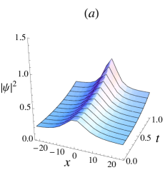
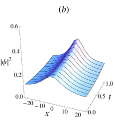
Figure 2: Intensity distribution of bright self-similar matter waves for $a_{1}=0.8$, $a_{2}=-1.2$, $a_{3}=0.09$ and for different values of ‘$a$’, as (a) $a=0.1$ and (b) $a=0.5$, respectively. The values of other parameters used in the plots are mentioned in the text.

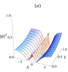
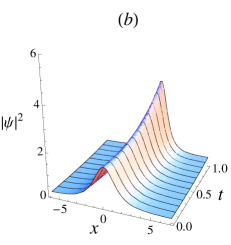
Figure 3: Intensity distribution of bright self-similar matter waves for $a=0.1$, $a_{1}=0.8$, and (a) $a_{2}=1.2$, $a_{3}=0.09$; (b) $a_{2}=-1.2$, $a_{3}=-0.09$. The other parameters chosen are same as in Fig. 2 (a).

For $a_{1}<0$ and $\epsilon>0$ which implies $\sigma>\frac{a_{2}^{2}}{3a_{1}}$, the cubic elliptic equation possesses dark soliton reads as [65]

$$\rho(x,t)=\sqrt{\frac{-\epsilon}{a_{1}}}\mbox{tanh}\Bigg{(}\sqrt{\frac{\epsilon}{\alpha^{2}}}\xi\Bigg{)},$$ (20)

with the same condition on source parameter as for bright soliton. Using Eq. (20) along with Eq. (14) and Eq. (11) into Eq. (4), the complex wave solution for Eq. (2) can be written as

$$\psi(x,t)=\frac{1}{W(t)}\Bigg{[}\sqrt{\frac{-\epsilon}{a_{1}}}\mbox{tanh}\Bigg{(}\sqrt{\frac{\epsilon}{\alpha^{2}}}\xi\Bigg{)}-\frac{a_{2}}{3a_{1}}\Bigg{]}~{}e^{i(k\chi-\omega\zeta+\phi(x,t))}.$$ (21)

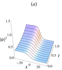
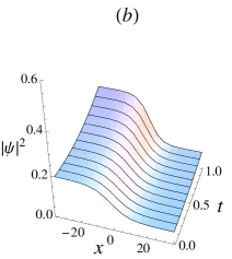
Figure 4: Intensity distribution of anti-kink self-similar matter waves for $a_{1}=-0.8$, $a_{2}=-1.2$, $a_{3}=0.09$ and for different values of ‘$a$’, as (a) $a=0.1$ and (b) $a=0.5$, respectively. The values of other parameters used in the plots are mentioned in the text.

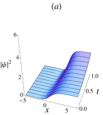
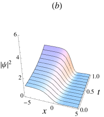
Figure 5: Intensity distribution of kink and anti-kink self-similar matter waves for $a=0.1$, $a_{1}=-0.8$, and (a) $a_{2}=1.2$, $a_{3}=0.09$; (b) $a_{2}=-1.2$, $a_{3}=-0.09$. The other parameters chosen are same as in Fig. 4(a).

We present the intensity distribution of these self-similar matter waves for same sign of nonlinearities and different values of ‘$a$’, as $a=0.1$ and $a=0.5$, respectively. As depicted in Figs. 4(a) and 4(b), we have anti-kink self-similar waves which are intensive for small values of ‘$a$’ as compared to large values. The other parameters are chosen as $a_{1}=-0.8$, $a_{2}=-1.2$, $a_{3}=0.09$, $v=1$, $\alpha=1$, $x_{0}=0$, $\zeta_{0}=0$ and $C_{02}=0.3$. In Fig. 5(a), we have shown the intensity distribution of self-similar matter wave, given by Eq. (21), for competitive nature of nonlinearities such as $a_{1}=-0.8$ and $a_{2}=1.2$. For this case, the profile of wave is reversed and one can observe the kink self-similar wave. Like bright self-similar matter waves, here also intensity of waves can be increased for negative value of source coefficient, as shown in the Fig. 5(b).

Lorentzian-type self-similar waves

For $\epsilon=0$ and $\delta=0$, Eq. (15) reduces to

$$\frac{1}{2}\alpha^{2}\rho^{\prime\prime}+a_{1}\rho^{3}+\eta\rho^{2}=0.$$ (22)

Eq. (22) have Lorentzian-type algebraic soliton solutions [66, 67] for $a_{1}>0$, expressed as

$$\rho(\xi)=\frac{P}{Q+\xi^{2}},$$ (23)

where $P=\frac{-3\alpha^{2}}{\eta}$ and $Q=\frac{9a_{1}\alpha^{2}}{4\eta^{2}}$. Subject to the conditions $\epsilon=\delta=0$, the parameters $\beta$ and $\sigma$ can be obtained from equations,

$$2a_{1}\beta^{3}+a_{2}\beta^{2}+a_{3}=0$$ (24)

and

$$\sigma=-(3a_{1}\beta^{2}+2a_{2}\beta),$$ (25)

respectively. Using Eq. (23) along with Eqs. (14) and (11) into Eq. (4), the complex wave solution for Eq. (2) can be written as

$$\psi(x,t)=\frac{1}{W(t)}\Bigg{(}\frac{P}{Q+\xi^{2}}+\beta\Bigg{)}~{}e^{i(k\chi-\omega\zeta+\phi(x,t))}.$$ (26)

The value of $\beta$ and $\sigma$ comes out from Eq. (24) and Eq. (25) by choosing values of model parameters $a_{1}$, $a_{2}$ and $a_{3}$ independently. Here, the constraint condition, $a_{1}>0$, is same as for bright self-similar matter wave discussed earlier. To study the difference between these two solution, we depicted the intensity distribution of Lorentzian-type self-similar matter waves in Fig. 6 (a), for same set of model parameters used in Fig. 2 (a), such as competitive nonlinearities $a_{1}=0.8$ and $a_{2}=-1.2$, and other parameters as $a_{3}=0.09$, $a=0.1$, $\omega=1.08$, $\alpha=1$, $\zeta_{0}=0$, $x_{0}=0$ and $C_{02}=0.3$. For these choices of model parameters, the scaling parameter found to be $\beta=0.04021$ and velocity of Lorentzian-type self-similar matter wave is $v=1.003$, compared to $v=1$ for Fig. 2 (a), which further modulates the parameter $k$ in the model equation, arises in the phase relation $\theta(x,t)=k\chi-\omega\zeta+\phi(x,t)$, as $k=v$. It means the model Eq. (2) can have different profiles of bright solitons, as presented in the Fig. 2 (a) and Fig. 6 (a), for small variation in the parameter $k$ which modulates the amplitude and velocity of self-similar matter waves. Further, the Lorentzian-type self-similar matter waves are W-shaped for same sign of nonlinearities as shown in the Fig. 6 (b), for same set of model parameters as used for Fig. 3 (a), but having different values of $\omega$ and $v$, given by $\omega=0.72$ and $v=0.8758$ which further modulates the parameter ‘$k$’. Hence, small variation in $k$ modulates the amplitude and velocity of W-shaped self-similar waves.

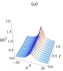
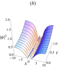
Figure 6: Intensity distribution of Lorentzian-type self-similar matter waves for $a=0.1$, $a_{1}=0.8$, $a_{3}=0.09$ and for different values of $a_{2}$, as (a) $a_{2}=-1.2$ and (b) $a_{2}=1.2$, respectively. The values of other parameters used in the plots are mentioned in the text.

Rational dark self-similar waves

For all the parameters of Eq. (15) to be non-zero i.e. $\epsilon\neq 0$, $\eta\neq 0$, $\delta\neq 0$ , the Eq. (15) have rational dark soliton solution expressed as [19]

$$\rho(\xi)=\frac{p}{q+\mbox{sech}(r\xi)},$$ (27)

with the conditions given as

$$a_{1}=\frac{q^{2}r^{2}\alpha^{2}}{p^{2}}(q^{2}-1),~{}~{}\eta=\frac{3qr^{2}\alpha^{2}}{2p}(1-2q^{2}),$$ (28)

$$\epsilon=\frac{(6q^{2}-1)}{2}\alpha^{2}r^{2},~{}~{}\delta=pqr^{2}\alpha^{2}.$$ (29)

Using Eq. (27) along with Eqs. (14) and (11) into Eq. (4), the complex wave solution for Eq. (2) can be written as

$$\psi(x,t)=\frac{1}{W(t)}\Bigg{[}\frac{p}{q+\mbox{sech}(r\xi)}+\beta\Bigg{]}~{}e^{i(k\chi-\omega\zeta+\phi(x,t))}.$$ (30)

The Eqs. (28) and (29) can be solved to obtain the values of unknown parameters $p$, $q$ and $r$ along with one parametric condition. Here, we have presented an interesting case by assuming $q=1$ for which the cubic nonlinearity coefficient ‘$a_{1}$’ equals to zero and the systems induce only quadratic nonlinearity. For $q=1$, the values of other parameters $p$ and $r$ comes out to be $\frac{5\delta}{2\epsilon}$ and $\pm\sqrt{\frac{2\epsilon}{5\alpha^{2}}}$, respectively along with parametric condition $\eta=\frac{-6\epsilon^{2}}{25\delta}$. This condition fixes the value of $\sigma$ term which can be obtained from the following relation

$$\sigma=\frac{1}{12}\left(\beta a_{2}\pm 5\sqrt{\beta^{2}a_{2}^{2}-24a_{2}a_{3}}\right).$$ (31)

The magnitude of the $\sigma$ estimated to be $0.76589$ for the parameters $a_{1}=0$, $a_{2}=1.2$ and $a_{3}=-0.09$. The other parameters used are $\beta=0.5$, $v=1$, $\alpha=1$, $\zeta_{0}=0$, $x_{0}=0$ and $C_{02}=0.3$. The intensity plot of rational dark self-similar matter wave in the absence of cubic nonlinearity is shown in Fig. (7) for different value of parameter ‘$a$’. As depicted from Figs. 7 (a) and 7 (b), the self-similar matter wave gets more intensive for small values of ‘$a$’.

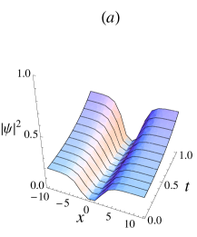
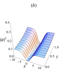
Figure 7: Intensity distribution of rational dark self-similar matter waves for $a_{1}=0$, $a_{2}=1.2$, $a_{3}=0.09$ and for different values of $a$, as (a) $a=0.1$ and (b) $a=0.5$, respectively. The values of other parameters used in the plots are mentioned in the text.

3.2 Gaussian-type trapping potential

For $W(t)=a+\text{exp}\left(-t^{2}\right)$, the trapping potential and gain / loss function [refer Eq. (10)] takes the form

$$f(t)=\frac{2(2t^{2}-1)}{1+a~{}e^{t^{2}}},h(t)=\frac{2t}{1+a~{}e^{t^{2}}}.$$ (32)

Figure 8: Profiles of trapping potential $f(t)$ and gain / loss function $h(t)$ for $a=0.1$.

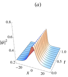
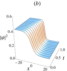
Figure 9: Intensity distribution of bright and kink self-similar matter waves for $a=0.1$, $a_{3}=0.09$ and for different nature of nonlinearities, as (a) $a_{1}=0.8$, $a_{2}=-1.2$ and (b) $a_{1}=-0.8$, $a_{2}=-1.2$, respectively. The values of other parameters used in the plots are mentioned in the text.

The profile of trapping potential and gain / loss function is presented in the Fig. (8), for $a=0.1$. It is clear that $f(t)$ is an even function and $h(t)$ is an odd function of time variable. For $a=0$, the quadratic nonlinearity turns out to be singular, so the parameter ‘$a$’ can take only non-zero values. But for this choice, it is not possible to solve variables $\zeta(t)$, $x_{c}(t)$ and $\phi(x,t)$ explicitly given by Eqs. (7) - (9), due to the presence of integral of reciprocal of width function. We solve the integral implicitly using numerical method to study the evolution of bright and kink self-similar waves for this choice of trapping potential. In Fig. (9), we depicted the intensity distribution of bright and dark self-similar matter waves for $a_{1}=0.8$, $a_{2}=-1.2$ and $a_{1}=-0.8$, $a_{2}=-1.2$, respectively. The other parameters used are $a=0.1$, $a_{3}=0.09$, $\alpha=1$, $v=1$, $x_{0}=0$, $\zeta_{0}=0$ and $C_{02}=0.3$. One can study the effect of parameter ‘$a$’ on the intensity of these waves and also observe the evolution of other self-similar waves for this trapping potential.

4 Conclusion

In conclusion, we have investigated the self-similar matter waves for driven GP equation with PT-symmetric potential in the presence of quadratic-cubic nonlinearity. Self-similarity transformation technique is employed to obtain bright, dark, Lorentzian-type and kink solitons under certain parametric constraints. The evolution of self-similar matter waves has been depicted for sech-type and Gaussian-type trapping potentials. We also have studied the effect of nature of nonlinearities, amplitude of trapping potential and source profile on the intensity of self-similar matter waves. Intensity can be made larger for specific choice of these parameters, resulting into generation of highly energetic self-similar waves in BEC.

5 Acknowledgment

S.P. would like to thank DST Inspire, India, for financial support through Junior Research Fellow [IF170725]. A.G. gratefully acknowledges Science and Engineering Research Board (SERB), Department of Science and Technology, Government of India for the award of SERB Start-Up Research Grant (Young Scientists) (Sanction No: YSS/2015/001803). H.K. is thankful to SERB-DST, India for the award of fellowship during the tenure of this work. We would like to thank Department of Physics, Panjab University for the research facilities.

References

- [1] M.H. Anderson, J.R. Ensher, M.R. Matthews, C.E. Wieman, E.A. Cornell, Science 269 (1995) 198.
- [2] K.B. Davis, M.O. Mewes, M.R. Andrews, N.J. VanDruten, D.S. Durfee, D.M. Kurn, W. Ketterle, Phys. Rev. Lett. 75 (1995) 3969.
- [3] F. Dalfovo, S. Giorgini, L.P. Pitaevskii, S. Stringari, Rev. Mod. Phys. 71 (1999) 463.
- [4] S.D. Nicola, B.A. Malomed, R. Fedele, Phys. Lett. A 360 (2006) 164.
- [5] D.S. Wang, X.H. Hu, J. Hu, W.M. Liu, Phys. Rev. A 81 (2010) 025604.
- [6] S. Inouye, M.R. Andrews, J. Stenger, H.J. Miesner, D. M. Stamper-Kurn, W. Ketterle, Nature 392 (1998) 151.
- [7] K.E. Strecker, G.B. Partridge, A.G. Truscott, R.G. Hule, New J. Phys. 5 (2003) 73.
- [8] S. Burger, K. Bongs, S. Dettmer, W. Ertmer, K. Sengstock, Phys. Rev. Lett. 83 (1999) 25.
- [9] X.Y. Tang, P.K. Shukla, Phys. Rev. A 76 (2007) 013612.
- [10] J.B. Beitia, J. Cuevas, J. Phys. A: Math. Theor. 42 (2009) 165201.
- [11] A.T. Avelar, D. Bazeia, W.B. Cardoso, Phys. Rev. E 79 (2009) 025602(R).
- [12] W.B. Cardoso, A.T. Avelar, D. Bazeia, Phys. Lett. A 374 (2010) 2640.
- [13] W.B. Cardoso, A.T. Avelar, D. Bazeia, Nonlinear Anal.-Real World Appl. 11 (2010) 4269.
- [14] C. Trallero-Giner, R. Cipolatti, T.C.H. Liew, Eur. Phys. J. D 67 (2013) 143.
- [15] U.A. Khawaja, H. Bahlouli, Commun. Nonlinear Sci. Numer. Simulat. 69 (2019) 248-260.
- [16] J. Fujioka, E. Cortes, R. Perez-Pascual, R.F. Rodriguez, A. Espinosa, B.A. Malomed, Chaos 21 (2011) 033120.
- [17] W.B. Cardoso, H.L.C. Couto, A.T. Avelar, D. Bazeia, Commun. Nonlinear Sci. Numer. Simulat. 48 (2017) 474.
- [18] H. Triki, A. Biswas, P. Seithuti, B. Moshokoa, M. Belic, Optik 128 (2017) 63.
- [19] R. Pal, H. Kaur, A. Goyal, C.N. Kumar, J. Mod. Opt. 66 (2019) 571.
- [20] R. Pal, S. Loomba, C.N. Kumar, D. Milovic, A. Maluckov, Ann. Phys. 401 (2019) 116.
- [21] P.G. Kevrekidis, D.J. Frantzeskakis, R. Carretero-González, B.A. Malomed, G. Herring, A.R. Bishop, Phys. Rev. A 71 (2005) 023614.
- [22] V.N. Serkin, A. Hasegawa, T.L. Belyaeva, Phys. Rev. Lett. 98 (2007) 074102.
- [23] A. Kundu, Phys. Rev. E 79 (2009) 015601(R).
- [24] A.T. Avelar, D. Bazeia, W.B. Cardoso, Phys. Rev. E 82 (2010) 057601.
- [25] P.K. Panigrahi, R.Gupta, A.Goyal, C.N. Kumar, Eur. Phys. J. Special Topics 222 (2013) 655.
- [26] T. Paul, P. Leboeuf, N. Pavloff, K. Richter, P. Schlagheck, Phys. Rev. A 72 (2005) 063621.
- [27] T. Paul, M. Hartung, K. Richter, P. Schlagheck, Phys. Rev. A 76 (2007) 063605.
- [28] T. Ernst, T. Paul, P. Schlagheck, Phys. Rev. A 81 (2010) 013631.
- [29] Z. Yan, X.F. Zhang, W.M. Liu, Phys. Rev. A 84 (2011) 023627.
- [30] T.S. Raju, P.K. Panigrahi, Phys. Rev. A 81 (2010) 043820.
- [31] T.S. Raju, P.K. Panigrahi, C.N. Kumar, J. Opt. Soc. Am. B 30 (2013) 934.
- [32] J.R. He, S. Xu, L. Xue, Phys. Scr. 94 (2019) 105216.
- [33] Z.H. Musslimani, K.G. Makris, R. El-Ganainy, D.N. Christodoulides, Phys. Rev. Lett. 100 (2008) 030402.
- [34] A. Khare, S.M. Al-Marzoug, H. Bahlouli, Phys. Lett. A 376 (2012) 2880.
- [35] Z.C. Wen, Z. Yan, Phys. Lett. A 379 (2015) 2025.
- [36] Y. Chen, Z. Yan, D. Mihalache, B.A. Malomed, Sci. Rep. 7 (2017) 1257.
- [37] C.Q. Dai, Y.J. Xu, Y. Wang, Commun. Nonlinear Sci. Numer. Simulat. 20 (2015) 389.
- [38] C.Q. Dai, X.G. Wang, G.Q. Zhou, Phys. Rev. A 89 (2014) 013834.
- [39] Y. Deng, S. Deng, C. Tan, C. Xiong, G. Zhang, Y. Tian, Opt. & Laser Technol. 79 (2016) 32.
- [40] C.M. Bender, S. Boettcher, Phys. Rev. Lett. 80 (1998) 5243.
- [41] C.M. Bender, D.C. Brody, H.F. Jones, Phys. Rev. Lett. 89 (2002) 270401.
- [42] R. El-Ganainy, K.G. Makris, D.N. Christodoulides, Z.H. Musslimani, Opt. Lett. 32 (2007) 2632.
- [43] Z.H. Musslimani, K.G. Makris, R. El-Ganainy, D.N. Christodoulides, Phys. Rev. Lett. 100 (2008) 030402.
- [44] K.G. Makris, R. El-Ganainy, D.N. Christodoulides, Z.H. Musslimani, Phys. Rev. Lett. 100 (2008) 103904.
- [45] V. Achilleos, P.G. Kevrekidis, D.J. Frantzeskakis, R. Carretero-Gonzalez, Phys. Rev. A 86 (2012) 013808.
- [46] H. Cartarius, G. Wunner, Phys. Rev. A 86 (2012) 013612.
- [47] F. Yu, L. Li, Nonlinear Dyn. 95 (2019) 1867.
- [48] F.K. Abdullaev, B.B. Baizakov, S.A. Darmanyan, V.V. Konotop, M. Salerno, Phys. Rev. A 64 (2001) 043606.
- [49] A.M. Kamchatnov, V.S. Shchesnovich, Phys. Rev. A 70 (2004) 023604.
- [50] B. Li, X.F. Zhang, Y.Q. Li, Y. Chen, W.M. Liu, Phys. Rev. A 78 (2008) 023608.
- [51] R. Balakrishnan, I.I. Satija, Pramana-J. Phy. 77 (2011) 929.
- [52] S. Coen, M. Haelterman, Phys. Rev. Lett. 87 (2001) 140401.
- [53] N. Dror, B.A. Malomed, J. Zeng, Phys. Rev. E 84 (2011) 046602.
- [54] A. Mohamadou, E. Wamba, D. Lissouck, T.C. Kofane, Phys. Rev. E 85 (2012) 046605.
- [55] D.B. Belobo, G.H. Ben-Bolie, T.C. Kofane, Phys. Rev. E 91 (2015) 042902.
- [56] C.N. Kumar, R. Gupta, A. Goyal, S. Loomba, Phys. Rev. A 86 (2012) 025802.
- [57] K.K De, A. Goyal, T.S. Raju, C.N. Kumar, P.K. Panigrahi, Opt. Commun. 341 (2015) 15.
- [58] A.M. Mateo, V. Delgado, Phys. Rev. A 77 (2008) 013617.
- [59] S. Sinha, L. Santos, Phys. Rev. Lett. 99 (2007) 140406.
- [60] S. Nixon and J. Yang, Phys. Rev. A 91 (2015) 033807.
- [61] S.A. Ponomarenko, G.P. Agrawal, Opt. Lett. 32 (2007) 1659.
- [62] A. Goyal, R. Gupta, S. Loomba, C.N. Kumar, Phys. Lett. A 376 (2012) 3454.
- [63] A.B. Shabat, V.E. Zakharov, Sov. Phys. JETP 34 (1972) 62.
- [64] H. Triki, K. Porseian, A. Choudhuri, P.T. Dinda, J. Mod. Opt. 64 (2017) 1368.
- [65] Y.S. Kivshar, B.L. Davies, Phys. Rep. 298 (1998) 81.
- [66] Alka, A. Goyal, R. Gupta, C.N. Kumar, Phys. Rev. A 84 (2011) 063830.
- [67] R. Pal, A. Goyal, S. Loomba, T.S. Raju, C.N. Kumar, J. Nonlin. Opt. Phys. Mat. 25 (2016) 1650033.