Science with the TianQin Observatory: Preliminary results on Galactic double white dwarf binaries

Abstract

We explore the prospects of detecting Galactic double white dwarf (DWD) binaries with the space-based gravitational wave (GW) observatory TianQin. In this work, we analyze both a sample of currently known DWDs and a realistic synthetic population of DWDs to assess the number of guaranteed detections and the full capacity of the mission. We find that TianQin can detect 12 out of $\sim 100$ known DWDs; GW signals of these binaries can be modeled in detail ahead of the mission launch, and therefore they can be used as verification sources. Besides, we estimate that TianQin has a potential to detect as many as $10^{4}$ DWDs in the Milky Way. TianQin is expected to measure their orbital periods and amplitudes with accuracies of $\sim 10^{-7}$ and $\sim 0.2$, respectively, and to localize on the sky a large fraction (39%) of the detected population to better than 1 deg². We conclude that TianQin has the potential to significantly advance our knowledge on Galactic DWDs by increasing the sample up to 2 orders of magnitude, and will allow their multi-messenger studies in combination with electromagnetic telescopes. We also test the possibilities of different configurations of TianQin: (1) the same mission with a different orientation, (2) two perpendicular constellations combined into a network, and (3) the combination of the network with the ESA-led Laser Interferometer Space Antenna. We find that the network of detectors boosts the accuracy on the measurement of source parameters by 1-2 orders of magnitude, with the improvement on sky localization being the most significant.

I Introduction

The first direct detection of gravitational waves generated from a binary black hole merger (GW150914) was made by the LIGO and Virgo Collaborations in 2015 Abbott et al. (2016a), one hundred years after they were predicted by Albert Einstein Einstein (1916). This detection, together with several subsequent ones including a binary neutron star merger (GW170817), started new fields of GW and multi-messenger astronomy Abbott et al. (2016b, 2019); The LIGO Scientific Collaboration et al. (2020); Abbott et al. (2020a, b).

The sensitivity band of the currently operational ground-based detectors LIGO and Virgo is limited between 10 Hz and kilohertz frequencies McWilliams et al. (2019). However, GW sources span many orders of magnitude in frequency down to femtohertz. Several experiments aim to cover such a large spectrum: the cosmic microwave background polarization experiments (Kamionkowski and Kovetz, 2016), the pulsar timing array (Arzoumanian et al., 2018; Shannon et al., 2015), and the space-based laser interferometers, sensitive to femtohertz, nanohertz and millihertz frequencies, respectively (Amaro-Seoane et al., 2017; Luo et al., 2016).

The millihertz frequency band is populated by a large variety of GW sources: massive black hole binaries ($10^{3}$ - $10^{7}\mathrm{M}_{\odot}$) formed via galaxy mergers Klein et al. (2016); Wang et al. (2019); Magorrian et al. (1998); Lynden-Bell (1969); Feng et al. (2019); compact stellar objects orbiting massive black holes, called extreme mass ratio inspirals (EMRIs) Babak et al. (2017); Fan et al. (2020); ultra-compact stellar mass binaries (and multiples) composed of white dwarfs, neutron stars and stellar-mass black holes in the neighborhood of the Milky Way Lamberts et al. (2018); Lau et al. (2020); Korol et al. (2017); Robson et al. (2018). Besides individually resolved binaries, stochastic backgrounds of astrophysical and cosmological origin can be detected at millihertz frequencies (e.g. Romano and Cornish, 2017; Liang et al., 2020). Therefore, this band is expected to provide rich and diverse science, ranging from Galactic astronomy to high-redshift cosmology and to fundamental physics Korol et al. (2018); Berti et al. (2005); Shi et al. (2019); Bao et al. (2019); Tamanini and Danielski (2018).

Among all kinds of ultra-compact stellar mass binaries, those composed of two white dwarf stars [double white dwarf binaries] comprise the absolute majority (up to $10^{8}$) in the Milky Way. Being abundant and nearby, DWDs are expected to be the most numerous GW sources for space-based detectors Nelemans et al. (2001a); Yu and Jeffery (2010); Breivik et al. (2019); Lamberts et al. (2018).

Individual GW detections of DWDs will significantly advance our knowledge on binary formation and white dwarf stars themselves in a number of ways. First, DWDs represent the end products of the low-mass binary evolution, and as such they encode information on physical processes such as the highly uncertain mass transfer and common envelope phases Postnov and Yungelson (2014); Belczynski et al. (2002). Second, DWDs are progenitors to AM canum venaticorum (AM CVn) systems, short-period ($\lesssim$1 hour) mass-transferring DWDs, ideal for studying the stability of the mass transfer Nelemans et al. (2001b); Marsh et al. (2004); Solheim (2010); Tauris (2018). Third, DWD mergers are thought to originate a broad range of interesting transient events including type-Ia supernovae (SNe Ia) Bildsten et al. (2007); Webbink (1984); Iben and Tutukov (1984); Webbink (1984). In addition, detached DWDs are particularly suitable for studying the physics of tides. DWDs affected by tides will yield information on the nature and origin of white dwarf viscosity, which is still a missing piece in our understanding of white dwarfs’ interior matter Piro (2011); Fuller and Lai (2012); Dall’Osso and Rossi (2014); Mckernan and Ford (2016). Finally, by analyzing their GW signals one could set constraints on deviations from general relativity Littenberg and Yunes (2019); Cooray and Seto (2004).

The overall GW signal from DWDs imprints the information on the Galactic stellar population as a whole, and it can constrain the structural properties of the Milky Way Benacquista and Holley-Bockelmann (2006); Adams et al. (2012); Korol et al. (2019); Breivik et al. (2019); Wilhelm et al. (2020). A significant fraction of the population may present a stellar or sub-stellar tertiary companions, that can be recognized by an extra frequency modulation of the DWD GW signals Robson et al. (2018); Tamanini and Danielski (2018); Steffen et al. (2018). GW detectors have the potential to guide the discovery of these populations Danielski et al. (2019).

TianQin is a space-based GW observatory sensitive to millihertz frequencies Luo et al. (2016); Yiming Hu (2019); Ye et al. (2019). Recently, a significant effort has been put into the study and consolidation of the science cases for TianQin Hu et al. (2017). On the astrophysics side, these efforts include studies on the detection prospect of massive black hole binaries Wang et al. (2019); Hu et al. (2018), EMRIs Fan et al. (2020), stellar-mass black hole binaries Liu et al. (2020), and stochastic backgrounds Liang et al. (2020); on the fundamental physics side, prospects for testing of the no-hair theorem with GWs from massive black hole binaries Shi et al. (2019) and constraints on modified gravity theories Bao et al. (2019); Xie et al. (2020); Liang et al. (2019); Zhang et al. (2020) have been assessed for TianQin. In this paper, we aim to forecast the detection of Galactic DWDs with TianQin. Due to their low masses, the GW horizon of DWDs is limited within the Milky Way, possibly reaching nearby satellite galaxies and the Andromeda galaxy Korol et al. (2018); Lamberts et al. (2018); Korol et al. (2020); Roebber et al. (2020). Therefore, in this study we focus on the Galactic population only. We concentrate on detached systems, because they are expected to be orders of magnitude more numerous than other types of binaries in the millihertz frequency regime (e.g., Nelemans et al., 2004; Nissanke et al., 2012).

The paper is organized as follows. In Section II, we outline the sample of the currently known ultra-compact DWDs and AM CVn’s, and we present a mock Galactic population. In Section III, we derive analytical expressions for computing the signal-to-noise ratio and uncertainties on binary parameters for TianQin. In Section IV, we present our results on the detectability of the known DWDs and that of the mock population. We also present similar results for some mission variations and explore the improvements that could be achieved when a few detectors work as a network. Finally, we summarize our main findings in Section V.

II Galactic Double White Dwarf Binaries

The currently known electromagnetic (EM) sample amounts to $\sim$100 detached and $\sim$60 interacting (AM CVn) DWD systems with orbital periods $\lesssim$1 day Brown et al. (2017); Maoz et al. (2018); Ramsay et al. (2018). Although rapidly expanding with several recent detections (Burdge et al., 2019a, b; Coughlin et al., 2020; Brown et al., 2020), this sample is still limited and represents only the tip of the iceberg of the overall Galactic population. To quantify the ability of TianQin in detecting DWDs, in this study we consider both the known sample and a synthetic Galactic population. In this section, we briefly outline both samples.

II.1 Candidate verification binaries

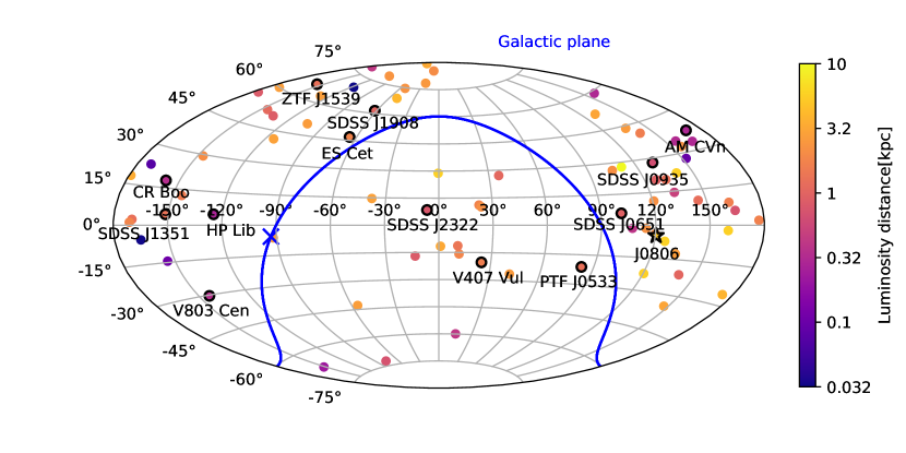
Figure 1: Sky positions of the 81 candidate verification binaries shown in the ecliptic coordinate system, with lighter colors representing shorter distances to the Solar System. Binaries with the highest SNR are highlighted. The blue line indicates the Galactic plane, with the Galactic Center marked by the blue cross.

Binaries discovered through EM observations are often called verification binaries in the literature (e.g. Stroeer and Vecchio, 2006; Kupfer et al., 2018). This is because we can measure their parameters and therefore accurately model their GW signals; the predicted signal can be used to verify the detector’s performance. Here we consider a sample of 81 candidate verification binaries (CVBs) (40 AM CVn type systems and 41 detached DWDs) with orbital periods $\lesssim$5 hours. FIG. 1 shows the sky positions and the luminosity distances of our CVBs in the ecliptic coordinate system.

We list parameters of verification binaries in Table LABEL:tb:VB_parameter in Appendix A. Parameters with poor observational constraints have been inferred from theoretical models. For example, for most verification binaries, trigonometric parallaxes from Gaia Data Release 2 (Gaia Collaboration et al., 2018) can be used to determine their luminosity distance Kupfer et al. (2018). Distances to RX J0806.3+1527 (also known as HM Cancri, hereafter J0806 Strohmayer (2005)), CR Boo, V803 Cen, SDSS J093506.92+441107.0, SDSS J075552.40+490627.9, SDSS J002207.65–101423.5 and SDSS J110815.50+151246.6, however, are determined using different methods. In particular, J0806 has a largely uncertain distance. Here we use a conservative upper boundary of 5 kpc based on its luminosity observation Roelofs et al. (2010).

In this work we define a DWD system as a verification binary if (1) it has been detected in the electromagnetic (EM) bands, and (2) its expected GW signal-to-noise ratio (SNR) for TianQin is $\geq$ 5 with a nominal mission lifetime of five years Stroeer and Vecchio (2006); Kupfer et al. (2018). We adopt a relatively low SNR threshold for the detection of the verification binaries, because there is a priori information from the EM observations to fall back on. We also define the potential verification binaries to be the CVBs which have $3\leq$ SNR $<5$ Stroeer and Vecchio (2006); Kupfer et al. (2018).

II.2 Synthetic Galactic population

In this study, we employ a synthetic catalog of Galactic DWDs based on models of Toonen et al. (2012, 2017). These models are constructed on a statistically significant number of progenitor zero-age main sequence systems $(\sim 10^{5})$ evolved with binary population synthesis code SeBa Portegies Zwart and Verbunt (1996) until both stars become white dwarfs. To construct the progenitor population the mass of the primary star is drawn from the Kroupa initial mass function in the range between 0.95 and 10 M_⊙ Kroupa et al. (1993). Then, the mass of the secondary is drawn from a uniform mass ratio distribution between 0 and 1 Duchêne and Kraus (2013). Orbital separations and eccentricities are obtained from a the log-flat distribution (considering those binaries that on the zero-age main sequence have orbital separations up to $10^{6}\,R_{\odot}$.) and a thermal distribution, respectively Abt (1983); Heggie (1975); Duchêne and Kraus (2013). The binary fraction is set to 50% and the metallicity to solar. It is important to note that in this paper we use models that employ the $\alpha\gamma-$common envelope evolution model designed and fine-tuned on observed DWDs Nelemans et al. (2000, 2001b). We highlight that this model matches well the mass ratio distribution (Toonen et al., 2012) and the number density (Toonen et al., 2017) of the observed DWDs.

Next, we assign the spatial and the age distributions to synthetic binaries. Specifically, we use a smooth Milky Way potential consistent of an exponential stellar disc and a spherical central bulge, adopting scale parameters as in (Korol et al., 2019, see table 1 of that source). The stellar density distribution is normalized according to the star formation history numerically computed by Boissier and Prantzos (1999), while the age of the Galaxy is set to $13.5\,$Gyr. We account for the change in binary orbital periods due to GW radiation from the moment of DWD formation until $13.5\,$Gyr.

Finally, for each binary we assign an inclination angle $\iota$, drawn randomly from a uniform distribution in $\cos\iota$. The polarization angle and the initial orbital phase ($\psi_{S}$ and $\phi_{0}$, respectively) are randomized, assuming uniform distribution over the intervals of [0, $\pi$) and [0, 2$\pi$), respectively. The obtained catalog contains the following parameters: orbital period $P$, component masses $m_{1}$ and $m_{2}$, the ecliptic latitude $\lambda$ and longitude $\beta$, distance from the Sun $d$, and angles $\iota,\psi_{S},\phi_{0}$. This catalog has been originally employed in the study of DWD detectability with LISA (Amaro-Seoane et al., 2017). Therefore, this paper represents a fair comparison with the results in Amaro-Seoane et al. (2017).

III Signal and noise modeling

III.1 Gravitational wave signals from a monochromatic source

The timescale on which DWDs’ orbits shrink via GW radiation is typically $>$ Myr (at low frequencies). This is significantly greater than the mission lifetime of TianQin of several years; the two timescales are only comparable when $f/\dot{f}\sim T_{\mathrm{m}}$:

$$f=0.18\left(\frac{T_{\mathrm{m}}}{5\mathrm{yr}}\right)^{-3/8}\left(\frac{\mathcal{M}}{1M_{\odot}}\right)^{-5/8}\mathrm{Hz}$$ (1)

Therefore, binaries with frequencies significantly smaller than 0.18 Hz can be safely considered as monochromatic GW sources, meaning that they can be described by a set of seven parameters: the dimensionless amplitude $(\mathcal{A})$, GW frequency $f=2/P$, $\lambda$, $\beta$, $\iota$, $\psi_{S}$ and $\phi_{0}$. Note that we do not include eccentricity because DWDs circularize during the common envelope phase.

GWs emitted by a monochromatic source can be computed using the quadrupole approximation Landau and Lifshitz (1962); Peters and Mathews (1963). In this approximation, the GW signal can be described as a combination of the two polarizations ($+$ and $\times$):

$$h_{+}(t)=\mathcal{A}(1+\cos\iota^{2})\cos(2\pi ft+\phi_{0}+\Phi_{D}(t))\,,$$ (2)

$$h_{\times}(t)=2\mathcal{A}\cos\iota\sin(2\pi ft+\phi_{0}+\Phi_{D}(t))\,,$$ (3)

with

$$\mathcal{A}=\frac{2(G\mathcal{M})^{5/3}}{c^{4}d}(\pi f)^{2/3},$$ (4)

where $\mathcal{M}\equiv(m_{1}m_{2})^{3/5}/(m_{1}+m_{2})^{1/5}$ is the chirp mass, and $G$ and $c$ are the gravitational constant and the speed of light, respectively. Note that the additional term $\Phi_{D}(t)$ in the GW phase [Eq. (2)-(3)] is the Doppler phase arising from the periodic motion of TianQin around the Sun:

$$\Phi_{D}(t)=2\pi ft\frac{R}{c}\sin(\pi/2-\beta)\cos(2\pi f_{m}t-\lambda)\,,$$ (5)

where $R=1\mathrm{A.U.}$ is the distance between the Earth and the Sun, and $f_{m}=1/\mathrm{year}$ is the modulation frequency. $\lambda$ and $\beta$ are the ecliptic coordinates of the source.

III.2 Detector’s response to GW signals

The design of the TianQin mission Luo et al. (2016) envisions a constellation of three drag-free satellites orbiting the Earth, maintaining a distance between each other of $\sim 10^{5}$ km. Satellites will form an equilateral triangle constellation oriented in such a way that the normal vector to the detector’s plane is pointing towards J0806 ($\lambda=120.4^{\circ}$, $\beta=-4.7^{\circ}$).

Configuration	TianQin
Number of satellites	N=3
Orientation	$\lambda=120.4^{\circ}$, $\beta=-4.7^{\circ}$
Observation windows	2 $\times$ 3 months each year
Mission lifetime	5 years
Arm length	$L=\sqrt{3}\times 10^{5}\mathrm{km}$
Displacement measurement noise	$S_{x}=1\times 10^{-24}\mathrm{m}^{2}\mathrm{Hz}^{-1}$
Acceleration noise	$S_{a}=1\times 10^{-30}\mathrm{m}^{2}\mathrm{s}^{-4}\mathrm{Hz}^{-1}$

Table 1: Key parameters for the TianQin configurations.

In the low-frequency limit ($f\ll f_{*}$ with $f_{*}=c/2\pi L$ being the transfer frequency, $\sim 0.28$ Hz for TianQin), the GW strain recorded by the detector can be described as a linear combination of the two GW polarizations modulated by the detector’s response Cutler (1998):

$$h(t)=h_{+}(t)F^{+}(t)+h_{\times}(t)F^{\times}(t)\,,$$ (6)

where $F^{+,\times}(t)$ are the antenna pattern functions.

For a detector with an equilateral triangle geometry, two orthogonal Michelson signals can be constructed and the antenna pattern functions can be expressed as

$$F^{+}_{\mathrm{1}}(t,\theta_{S},\phi_{S},\psi_{S}) = \frac{\sqrt{3}}{2}\Bigg{(}\frac{1}{2}(1+\cos^{2}\theta_{S})\cos 2\phi_{S}(t)\cos 2\psi_{S}-\cos\theta_{S}\sin 2\phi_{S}(t)\sin 2\psi_{S}\Bigg{)}\,,$$ (7)

$$F^{\times}_{\mathrm{1}}(t,\theta_{S},\phi_{S},\psi_{S}) = \frac{\sqrt{3}}{2}\Bigg{(}\frac{1}{2}(1+\cos^{2}\theta_{S})\cos 2\phi_{S}(t)\sin 2\psi_{S}+\cos\theta_{S}\sin 2\phi_{S}(t)\cos 2\psi_{S}\Bigg{)}\,,$$ (8)

$$F^{+}_{\mathrm{2}}(t,\theta_{S},\phi_{S},\psi_{S}) = F^{+}_{\mathrm{1}}(t,\theta_{S},\phi_{S}-\frac{\pi}{4},\psi_{S})\,,$$ (9)

$$F^{\times}_{\mathrm{2}}(t,\theta_{S},\phi_{S},\psi_{S}) = F^{\times}_{\mathrm{1}}(t,\theta_{S},\phi_{S}-\frac{\pi}{4},\psi_{S})\,,$$ (10)

where $\sqrt{3}/2$ represents a factor originating from the geometry of the detector and encodes the $60^{\circ}$ angle between the detector’s arms, and $\theta_{S}$ and $\phi_{S}(t)=\phi_{S0}+\omega t$ are the latitude and longitude of the source in the detector’s coordinate frame, with $\omega\approx 2\times 10^{-5}$ rad/s being the angular frequency of the TianQin satellites. The transformation from the ecliptic coordinates ($\beta,\lambda$) to the detector coordinates ($\theta_{S},\phi_{S}$) can be found in Appendix E. The subscripts 1 and 2 in Eqs. (7)-(10) are labels for the two Michelson signals, which are orthogonal to each other, as indicated by the $\pi/4$ phase difference between the corresponding antenna pattern functions (e.g., Cutler, 1998). From Eqs. (7)-(10) one can conclude that TianQin is most sensitive to GWs propagating along the normal direction to the detector’s plane, and least sensitive to GWs propagating along the detector plane.

In general, the exact inclusion of the antenna pattern functions is complicated (e.g., Cornish and Rubbo, 2003). In practice, we introduce the sky-averaged response function $R(f)$ to simplify the following calculations. It can be approximated by

$$R(f)\approx\frac{3}{10}\frac{1}{1+0.6(f/f_{*})^{2}}\,.$$ (11)

The prefactor $3/10=2\times 3/20$ is two times (to account for two independent Michelson interferometers) the sky-averaged factor of $3/20$, which can be obtained as $\overline{F^{\times,+}}$, with $\overline{F^{\times,+}}\equiv\frac{1}{4\pi^{2}}\int^{\pi}_{0}\mathrm{d}\psi_{S}\int^{2\pi}_{0}\mathrm{d}\phi\int^{\pi}_{0}F^{\times,+}\sin\theta\mathrm{d}\theta$.

III.3 Detector noise and the scaled sensitivity curve

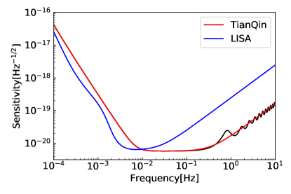
Figure 2: The sensitivity curve of TianQin. The red line corresponds to $\tilde{S}_{n}(f)$, defined in Eq. (13), while the black line corresponds to the full sky-averaged result, preserving all the frequency dependence (see Eqs. (15)-(16) in Wang et al. (2019)). The LISA sensitivity curve is shown by the blue line according to Robson et al. (2019).

The huge number of Galactic DWDs can generate a foreground confusion noise that may affect the detection of other types of GW sources. In Sect. IV.1 we show that such foreground is relatively weak for TianQin. Therefore, through this paper we only consider the instrumental noise.

The noise spectral density of TianQin can be expressed analytically as

$$S_{N}(f) = \frac{1}{L^{2}}\left[\frac{4S_{a}}{(2\pi f)^{4}}\left(1+\frac{10^{-4}{\rm Hz}}{f}\right)+S_{x}\right],$$ (12)

where $L$, $S_{a}$, $S_{x}$ are given in Table 1.

From the sky-averaged response function Eq. (11) and the detector noise Eq. (12), one can construct the sensitivity curve of the detector as

$$\tilde{S}_{n}(f) = S_{N}(f)\Big{/}\tilde{R}(f)$$ (13)

$$= \frac{1}{L^{2}}\left[\frac{4S_{a}}{(2\pi f)^{4}}\left(1+\frac{10^{-4}Hz}{f}\right)+S_{x}\right]$$

$$\times\left[1+0.6\left(\frac{f}{f_{*}}\right)^{2}\right]\,,$$

where

$$\tilde{R}(f)\equiv R(f)\frac{10}{3}=\frac{1}{1+0.6(f/f_{*})^{2}}\,.$$ (14)

Note that in this formalism, we assume the effect of the antenna pattern to be associated with the signal. The obtained sensitivity curve is represented in FIG. 2.

III.4 Data analysis

The SNR $\rho$ of a signal is defined as

$$\rho^{2}=(h|h),$$ (15)

where the inner product $(\cdot|\cdot)$ is defined as Finn (1992); Cutler and Flanagan (1994),

$$(a|b) = 4\Re e\int^{\infty}_{0}\mathrm{d}f\frac{\tilde{a}^{*}(f)\tilde{b}(f)}{\tilde{S}_{n}(f)}$$ (16)

$$\simeq \frac{2}{\tilde{S}_{n}(f_{0})}\int^{T}_{0}\mathrm{d}t\,a(t)b(t),$$

where $\tilde{a}(f)$ and $\tilde{b}(f)$ are the Fourier transformations of two generic functions $a(t)$ and $b(t)$, $\tilde{S}_{n}(f)$ is defined in Eq. (13). The second step is obtained by using Parseval’s theorem and the quasi-monochromatic nature of the signal, which acts like a Dirac delta function on the noise power spectral density Cutler (1998).

For a monochromatic GW signal with frequency $f_{0}$, it is possible to derive an analytical expression of the SNR ($\rho$)

$$\rho^{2}=(h|h)\simeq\frac{2}{\tilde{S}_{n}(f_{0})}\int^{T}_{0}\mathrm{d}t\,h(t)h(t)=\frac{2\langle A^{2}\rangle T}{\tilde{S}_{n}(f_{0})}\,,$$ (17)

with

$$\langle A^{2}\rangle = \frac{1}{T}\int^{T}_{0}h^{2}(t)\,\mathrm{d}t.$$ (19)

$$\approx \frac{3}{16}\mathcal{A}^{2}\Big{[}(1+\cos^{2}\iota)^{2}\langle F_{+}^{2}\rangle$$

$$\qquad\quad+4\cos^{2}\iota\langle F_{\times}^{2}\rangle\Big{]},$$

$$\langle F_{+}^{2}\rangle = \frac{1}{4}(1+\cos^{2}\theta_{S})^{2}\cos^{2}2\psi_{S}$$ (20)

$$+\cos^{2}\theta_{S}\sin^{2}2\psi_{S},$$

$$\langle F_{\times}^{2}\rangle = \frac{1}{4}(1+\cos^{2}\theta_{S})^{2}\sin^{2}2\psi_{S}$$ (21)

$$+\cos^{2}\theta_{S}\cos^{2}2\psi_{S}\,,$$

where $T$ is the observation time (which is half the operation time), and we have neglected the $\mathcal{O}(T^{-1})$ terms in Eq. (19). It is also useful to define the characteristic strain $h_{c}=A\sqrt{N}$, with $N=f_{0}T$ being the number of binary orbital cycles observed during the mission. Analogously, the noise characteristic strain is $h_{n}(f)=\sqrt{f\tilde{S}_{n}(f)}$. One can straightforwardly estimate the SNR from the ratio between $h_{c}$ and $h_{n}$.

III.5 Galactic GW foreground

At frequencies $<1$ mHz, the number of Galactic sources per frequency is too large to resolve all individual GW signals. These signals can potentially become indistinguishable and form a foreground for the TianQin mission (in analogy with Cornish and Robson, 2017). We assess the level of such a foreground using a synthetic population presented in Section II.2.

We follow the method outlined in Littenberg and Cornish (2015). For each binary, we construct the signal in the frequency domain, $h(f)$ (cf. Section III.1). All signals in each frequency bin are then incoherently added, forming an overall population spectrum. Next, we smooth the spectrum by a running median smoothing function with a set window size and by fitting with cubic spline to it. We define the smoothed Galactic spectrum $S_{\rm DWD}(f)$ and compute the total noise as the sum of the instrumental noise $S_{n}(f)$ and $S_{\rm DWD}(f)$. Using the updated noise curve, we check if any DWDs results have a SNR larger than the preset threshold of 7. These “resolved” DWDs are then removed from the sample, and the process is repeated from the beginning. The iterations are performed until the convergence i.e., until there are no more new resolved sources. The final result is represented in FIG. 3.

Table 2: The coefficients for the polynomial fit for the foreground, as $10^{\sum_{i}a_{i}x^{i}}$, where $x=\log{(f/10^{-3})}$. Successive rows correspond to increasing operation time $T$.

$T$	$a_{0}$	$a_{1}$	$a_{2}$	$a_{3}$	$a_{4}$	$a_{5}$	$a_{6}$
0.5 yr	-18.6	-1.22	0.009	-1.87	0.65	3.6	-4.6
1 yr	-18.6	-1.13	-0.945	-1.02	4.05	-4.5	-0.5
2 yr	-18.6	-1.45	0.315	-1.19	-4.48	10.8	-9.4
4 yr	-18.6	-1.43	-0.687	0.24	-0.15	-1.8	-3.2
5 yr	-18.6	-1.51	-0.710	-1.13	-0.83	13.2	-19.1

III.6 Parameter estimation

The uncertainty on the binary parameters can be derived from the Fisher information matrix (FIM) $\Gamma_{ij}$,

$$\Gamma_{ij}=\left(\frac{\partial h}{\partial\xi_{i}}\bigg{|}\frac{\partial h}{\partial\xi_{j}}\right),$$ (22)

where $\xi_{i}$ stands for the $i{\rm th}$ parameter.

In the high-SNR limit ($\rho\gg$ 1), the inverse of the FIM equals to the variance-covariance matrix, $\Sigma=\Gamma^{-1}$. The diagonal entries $\Sigma_{ii}$ give the variances (or mean square errors) of each parameter, $(\Delta\xi_{i})^{2}$, while the off-diagonal entries describe the covariances. In numerical calculations, we approximate $\partial h/\partial\xi_{i}$ with numerical differentiation

$$\frac{\partial h}{\partial\xi_{i}}\approx\frac{\delta h}{\delta\xi_{i}}\equiv\frac{h(t,\xi_{i}+\delta\xi_{i})-h(t,\xi_{i}-\delta\xi_{i})}{2\delta\xi_{i}}\,.$$ (23)

The differentiation steps $\delta\xi_{i}$ were chosen to make the numerical calculation stable Shah et al. (2012).

Notice that compared with the uncertainty of each coordinate, we are more interested in the sky localization, which is a combination of the uncertainties of both coordinates Cutler (1998):

$$\Delta\Omega_{\rm S}=2\pi\big{|}\sin\beta\big{|}\big{(}\Sigma_{\beta\beta}\Sigma_{\lambda\lambda}-\Sigma^{2}_{\beta\lambda}\big{)}^{1/2}\,.$$ (24)

When a network of independent detectors is considered, the total SNR and FIM of a source can be calculated as

$$\rho^{2}_{\mathrm{total}} = \sum_{a}\rho^{2}_{a}=\sum_{a}(h_{a}|h_{a})\,,$$

$$\Gamma_{\mathrm{total}} = \sum_{a}\Gamma_{a}=\sum_{a}\left(\frac{\partial h_{a}}{\partial\xi_{i}}\bigg{|}\frac{\partial h_{a}}{\partial\xi_{j}}\right)\,,$$ (25)

where the subscript $a$ stands for quantities related to the $a{\rm th}$ detector.

IV Results

In this section we report our results for the TianQin mission. We also consider an alternative version of the mission configuration with the same characteristics (cf. Table 1), but oriented perpendicularly to the original TianQin’s configuration (pointing towards $\lambda=30.4^{\circ}$ and $\beta=0^{\circ}$). In the following, we denote the standard TianQin configuration as TQ and the additional one as TQ II. GW observations can be improved if many detectors are working simultaneously in a network (e.g., the LIGO + Virgo network). Therefore, in this work we also explore the possibility of two detectors TQ and TQ II operating simultaneously, both following the “three months on + three months off” observation scheme as a way to fill the data gaps of each other. We refer to the configuration consisting of the two detectors as TQ I+II. In addition, we also explore the possibility of TQ and TQ I+II operating together with LISA.

IV.1 Galactic foreground

First, we assess the impact of the Galactic confusion foreground for TianQin. In FIG. 3, we show the estimates of the foreground levels corresponding to different operation times (colored lines) obtained according to the procedure described in Section IV.1. Each line can be reproduced by using the expression $S_{\rm DWD}(f)=10^{\sum_{i}a_{i}x^{i}}$, where $x=\log{(f/10^{-3})}$ and polynomial coefficients $a_{i}$ are reported in Table 2 for different operation times.

From FIG. 3, it is evident that the foreground strain is inversely proportional to the operation time. Therefore we did not include the Galactic foreground in the following analysis. Notice that the foreground of TianQin and TianQin II are quite consistent, so change in orientation has relatively minor effect on the overall foreground. This is illustrated in FIG. 3 where foreground of TQ II for 5 year operation time is shown.

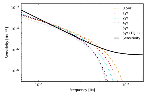
Figure 3: Expected foreground from Galactic DWDs for different operation times (colored lines). The black solid line represents the sensitivity curve of TianQin (cf. FIG. 2). The foreground with a 5 year operation time for TianQin II is also shown for comparison. Notice that it is consistent with the foreground of the TianQin constellation with the same operation time.

IV.2 Verification binaries

Out of 81 considered candidates (cf. Table LABEL:tb:VB_parameter) we find 12 verification binaries with SNR$\geq 5$: J0806, V407 Vul, ES Cet, AM CVn, SDSS J1908, HP Lib, CR Boo, V803 Cen, ZTF J1539, SDSS J0651, SDSS J0935, and SDSS J2322, with J0806 having the highest SNR. In particular, we find that J0806 reaches a SNR threshold of 5 already after only two days of observation. We predict that its SNR will reach 36.8 after three months of observation, and will exceed 100 after nominal five years of mission (effectively corresponding to 2.5 years of observation time). In addition, we find three potential verification binaries with 3 $\leq$ SNR $<$ 5: SDSS J1351, CXOGBS J1751 and PTF J0533. Figure 4 shows the evolution of the SNR with time for all verification binaries in blue for TianQin (TQ).

In Table LABEL:tb:VB_SNR, we report dimensionless amplitudes ($\mathcal{A}$) and SNRs for all 81 CVBs considering mission configurations: TianQin (TQ), TQ II, and TQ I+II, assuming five years of mission lifetime and setting $\phi_{0}=\pi$ and $\psi_{S}=\pi/2$ for all binaries. We note that the sky position, orbital inclination and GW frequency of the binary affect SNR by a factor of a few (cf. Eqs.(17)-(21)). For example, V803 Cen and SDSS J0651 have comparable GW amplitudes ($16.0\times 10^{-23}$ and $16.2\times 10^{-23}$, respectively), but their SNRs differ significantly (6.2 and 26.5, respectively). This difference arises both from the fact that SDSS J0651 is located in a more favorable position in the sky for TianQin (TQ), and the fact that it has a higher frequency than V803 Cen. We also note that because TianQin (TQ) is oriented directly towards J0806, its SNR is the largest across the sample, although its amplitude is not the highest. When considering the TQ II configuration with a different orientation, its SNR decreases by a factor of $\sim 3$.

We find that TQ II can detect 13 verification binaries with SNR$>5$ and one potential verification binary with 3 $<$ SNR $<$ 5. Being orthogonal to TianQin (TQ), the TQ II configuration is more disadvantageous than for the detection of J0806. However, even with TQ II, J0806 can be detected with a SNR of 41.6. This is because J0806 has the highest frequency across the sample (cf. Table LABEL:tb:VB_parameter). With a frequency of 6.22 mHz, it is positioned in the amplitude-frequency parameter space where the noise level of TianQin is the lowest (see also FIG. 5). Therefore, J0806 is still among the best verification sources for the TQ II configuration.

Similarly, for the network TQ I+II there will be 14 verification binaries and 1 potential verification binary. The SNR evolution for different operation times for these verification binaries is represented in red in FIG. 4. The SNR produced by a source in this case is given by the root sum squared of the SNRs of the two configurations considered independently (see Eq.(25)). Therefore, if TianQin (TQ) and TQ II independently detect a source with a similar SNR, the network TQ I+II would improve the SNR by a factor of $\sqrt{2}$. However, if the source produces significantly higher SNR in one of the detectors in the network, the improvement is not significant (e.g., J0806 in Table LABEL:tb:VB_SNR).

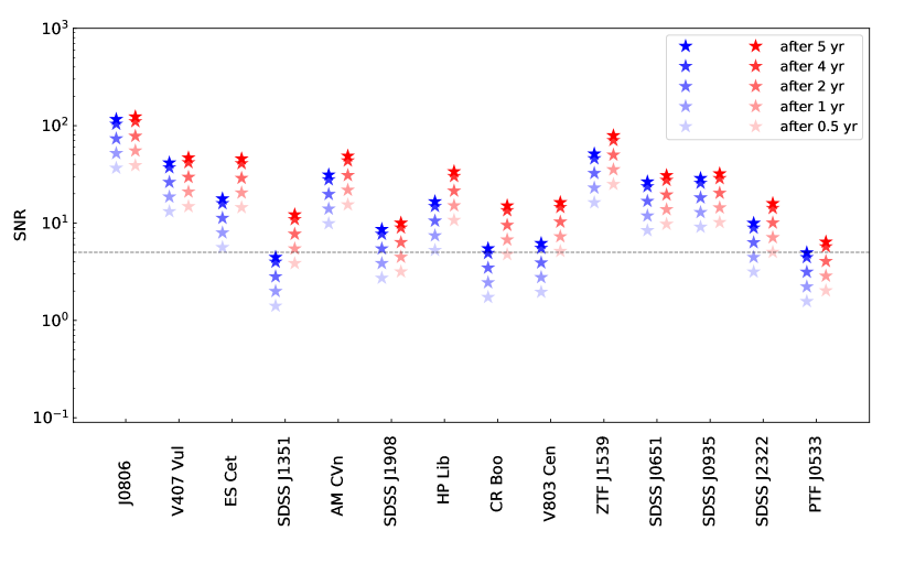
Figure 4: The SNR evolution of verification binaries over time. Blue stars represent TianQin (TQ), and red stars represent TQ I+II. The black dashed line corresponds to the SNR threshold of 5.

In Table 3, we fix all other parameters and only report the estimated uncertainties on the amplitude $\mathcal{A}$ and inclination angle $\iota$ for the 14 verification binaries. These two parameters are typically degenerate (cf. Eqs. (2)-(3)). However, for nearly edge-on binaries the degeneracy can be broken by using the asymmetry between two GW polarizations (e.g. Shah et al., 2012). We present TianQin’s ability to constrain the polarization angle $\psi$ in later sections. We remark that Xie et al. (2020) demonstrate that in the most favorable setup, TianQin has the potential to constrain the relative strength of extra polarization modes to the tensor modes at an accuracy of about $10^{-3}$. This is reflected in a small correlation coefficient $c_{\mathcal{A},\cos\iota}=0.157$ of SDSS J0651 with the inclination angle of $86.95^{\circ}$. For decreasing inclination angles the degeneracy increases as can be seen for SDSS J1908 and V803 Cen with inclination angles of $\iota=15^{\circ}$ and $\iota=13.5^{\circ}$ respectively. These two verification binaries have $\Delta{\cos\iota}>1$, meaning that the uncertainty on the inclination angle exceeds the physical range (0, $\pi$).

By means of like eclipsing binaries observations, the inclination angle can be independently determined from the EM channel. It can then be used to narrow down the uncertainty on the inclination from GW data by removing the respective row and column of the FIM. In the column denoted “With EM on $\iota$” in Table 3, we recalculate the uncertainties on the amplitude by inverting $\Gamma_{\mathcal{A}\mathcal{A}}$, equivalently assuming that the inclination of the binary is known by EM observation, and we report the ratio between this uncertainty and the uncertainty estimated without EM observation on $\iota$ (fourth column of Table 3). We find that, when the inclination angle is known a priori, the uncertainty on the amplitude can be improved up by to a factor of $\sim$ 16 (e.g., for SDSS J2322), depending on the exact value of the inclination angle of the source. Note that the improvement for nearly edge-on binaries (ZTF J1539 and SDSS J0651) is negligible.

Table 3: Uncertainties on $\mathcal{A}$ and $\iota$ for 14 verification binaries considering the TQ I+II configuration. In the column denoted “Without EM on $\iota$,” we report uncertainties on $\mathcal{A}$ and $\cos\iota$ derived from inverting the $2\times 2$ FIM. In the column denoted “With EM on $\iota$,” we report uncertainties on $\mathcal{A}$ for the case when $\iota$ is known a priori from EM observation.

Source	without EM on $\iota$			with EM on $\iota$
	$\Delta\mathcal{A}/\mathcal{A}$	$\Delta{\cos\iota}$	$c_{\mathcal{A},\cos\iota}$	$\Delta^{\prime}{\mathcal{A}}/\mathcal{A}$	$\Delta{\mathcal{A}}/\Delta^{\prime}{\mathcal{A}}$
J0806	0.061	0.055	0.991	0.008	7.625
V407 Vul	0.050	0.039	0.904	0.021	2.381
ES Cet	0.051	0.039	0.904	0.022	2.318
SDSS J1351	0.193	0.145	0.905	0.082	2.354
AM CVn	0.115	0.102	0.984	0.020	5.750
SDSS J1908	6.102	$>1$	1.000	0.100	$>1$
HP Lib	0.384	0.360	0.997	0.030	12.800
CR Boo	0.865	0.813	0.997	0.066	13.106
V 803 Cen	4.377	$>1$	1.000	0.062	$>1$
ZTF J1539	0.013	0.012	0.300	0.013	1.000
SDSS J0651	0.033	0.018	0.157	0.032	1.031
SDSS J0935	0.073	0.056	0.904	0.031	2.355
SDSS J2322	1.033	0.979	0.998	0.063	16.397
PTF J0533	0.219	0.137	0.700	0.156	1.404

IV.3 Simulated Galactic double white dwarf binaries

To forecast the total number of binaries detectable by TianQin we employ the simulated population of Galactic DWDs (cf. Sec. II.2). Here, we set a higher SNR threshold of 7, assuming that there is no a priori information from the EM observations to fall back on.

We estimate the number of resolved DWDs for the three considered configurations (TQ, TQ II, and TQ I+II) to be of the order of several thousand for the full mission lifetime of 5 years. In Table 4, we summarize our result for increasing operation times. In FIG. 5 we show the dimensionless characteristic strain of DWDs with SNR$>40$ in the mock population compared to 14 verification binaries.

The density of DWDs in the bulge region of the Galaxy is significantly higher than in the disk (see Fig. 3 of Korol et al. (2019)); therefore the detector’s orientation has a significant impact on the total number of detectable DWDs. The Galactic Center (where the density of DWDs is the highest) in ecliptic coordinates corresponds to $(\lambda=266.8^{\circ},\beta=-5.6^{\circ})$. TianQin (TQ) is oriented towards $(\lambda=120.4^{\circ},\beta=-4.7^{\circ}$) that is, about 30^∘ away from the Galactic Center; TQ II is oriented towards ($\lambda=30.4^{\circ},\beta=0^{\circ}$),which is about 60^∘ away from the Galactic Center. Consequently, the number of detected DWDs for TianQin (TQ) is about $1.3$-$1.4$ times larger than for TQ II (cf. Table 4). When we consider TQ I+II, the number of detections increases by $\sim 1.3$ compared to TianQin (TQ) alone. We verify that pointing the detector towards the Galactic Center would return the maximum detections $\sim 1.0\times 10^{4}$.

	0.5yr	1yr	2yr	4yr	5yr
TQ	2371	3589	5292	7735	8710
TQ II	1672	2595	3943	5782	6540
TQ I+II	3146	4716	6966	10023	11212

Table 4: The expected detection numbers of resolvable binaries for TianQin (TQ), TQ II, and TQ I+II.

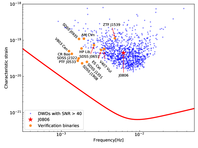
Figure 5: The characteristic strain $h_{c}$ of the 14 verification binaries (the golden dots and the red star) for TQ I+II and the simulated DWDs with SNR $>$ 40 for TianQin, compared with the noise amplitude $h_{n}$ of TianQin (red line). J0806 is highlighted with a red star. An operation time of 5 years is assumed.

FIG. 6 illustrates the distributions of the SNRs and relative uncertainties on binary parameters $\mathcal{A}$, $P$, $\cos{\iota}$, $\psi_{S}$, and sky position $\Omega_{\rm S}$ (Eq. 24). The figure shows that most sources have a relatively low SNR ($\lesssim$10), and that there is a non-negligible number of sources with SNR $>100$ reaching a maximum of $\sim 1000$. These high-SNR binaries are also well-localized ones (because $\Delta\Omega_{\rm S}\propto 1/\rho^{2}$); theretofore, they will be good candidates for EM follow-up and multi-messenger studies Littenberg et al. (2013). We find that for $90\%$ of detections, the uncertainty on $\Delta P/P$ falls within the range $(0.15-4.63)\times 10^{-7}$, on $\Delta\mathcal{A}/\mathcal{A}$ within $0.04-5.02$, on $\Delta\cos\iota$ within $0.02-4.95$, on $\Delta\psi_{S}$ within $0.03-4.01$ rad, and on $\Delta\Omega_{\rm S}$ within $0.02-21.36$ deg². The median values of these uncertainties are: $\Delta P/P=1.41\times 10^{-7}$, $\Delta\mathcal{A}/\mathcal{A}=0.26$, $\Delta\cos\iota=0.20$, $\Delta\psi_{S}=0.39$ rad, and $\Delta\Omega_{\rm S}=1.85$ deg². We highlight that TianQin (TQ) can locate 39% of DWDs to within better than 1 deg², while TQ I+II can locate 54% of detections within 1 deg².

Next, we explore the additional cases of TianQin operating in combination with LISA: TQ + LISA and TQ I+II + LISA. For these additional cases, the mission lifetimes of TQ and TQ I+II are assumed to be 5 years, while that for LISA is taken to be 4 years (Amaro-Seoane et al., 2017). We verify that by adding LISA to the network, the total number of detected DWDs doubles. This is due to the fact that LISA is sensitive to relatively lower GW frequencies, where the number of DWDs is larger.

As shown in Eq. (25), an additional detector can increase the SNR of a source, and parameter estimation can also benefit. We also look at the improvement in the parameter estimation precision for the 8710 resolvable binaries for TianQin. In FIG. 7, we present the histograms of the ratio between the uncertainties when measured by TianQin alone, and when measured by a network of detectors. The top left panel of FIG. 7 shows that the improvement on the SNR is within a factor of 10, while the improvements on the parameters uncertainties are within a factor of a few dozens for $\cos{\iota}$ and $\mathcal{A}$ and are largely comparable for all three networks. Improvements on the SNR, $\mathcal{A}$, $P$, $\psi_{S}$, and $\Omega_{\rm S}$ are larger for TQ + LISA and TQ I+II + LISA; those on $\psi_{S}$ and $\Omega_{\rm S}$ can reach up to 2 or 3 orders of magnitude.

We remark that (1) TQ + LISA and TQ I+II + LISA are better than TianQin and TQ I+II in determining DWDs’ periods. (2) TianQin and TQ I+II are slightly better than TQ + LISA and TQ I+II + LISA in determining GW amplitudes and $\cos(\iota)$. (3) TQ I+II is better than TQ + LISA and TQ I+II + LISA, and the latter two are better than TianQin in determining the sky positions. (4) The result for the polarization angle $\psi_{S}$ is a bit mixed, but the three networks of detectors usually perform better than TianQin alone.

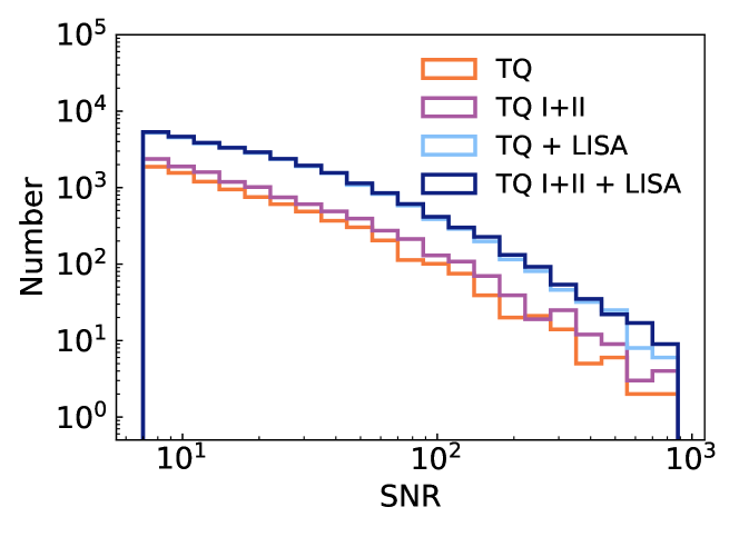
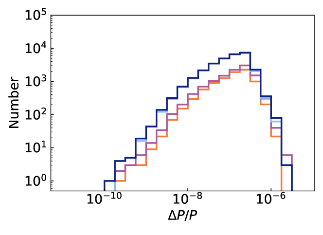
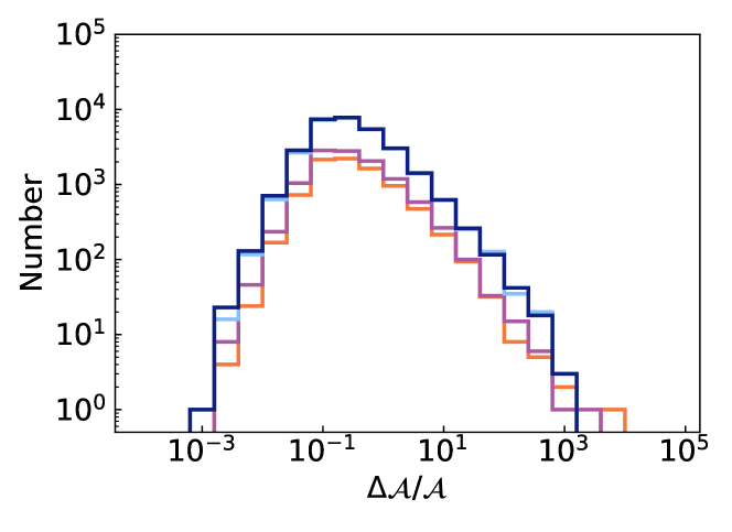
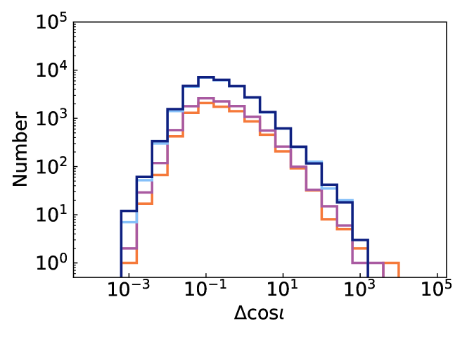
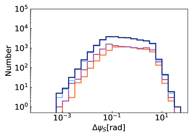
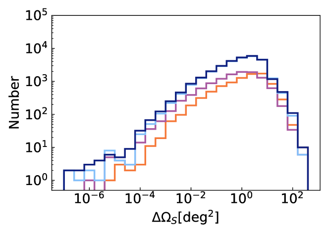
Figure 6: The histograms (un-normalized) for the SNR and the uncertainties of parameter estimation for the resolvable binaries of different detection scenarios with TianQin (orange), TQ I+II (magenta), TQ + LISA (light blue) and TQ I+II + LISA (blue).

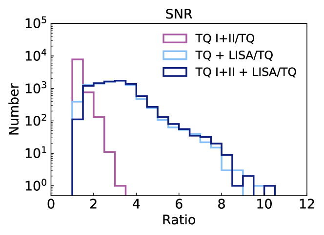
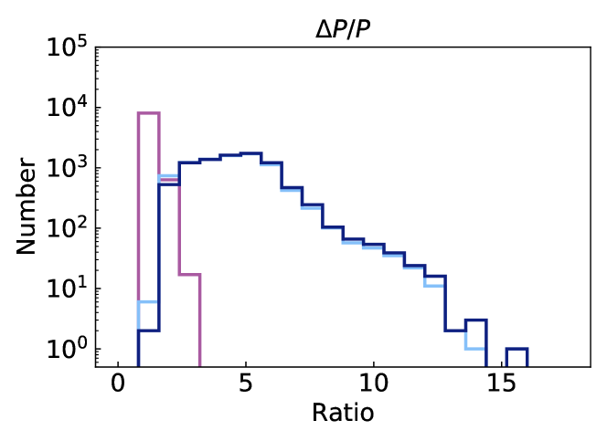
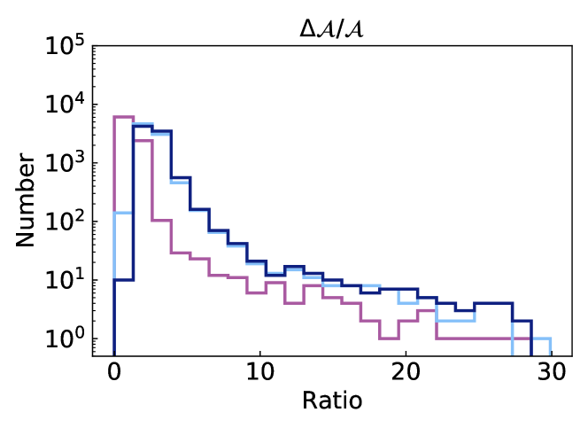
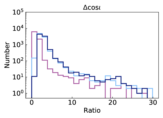
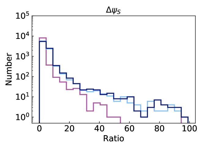
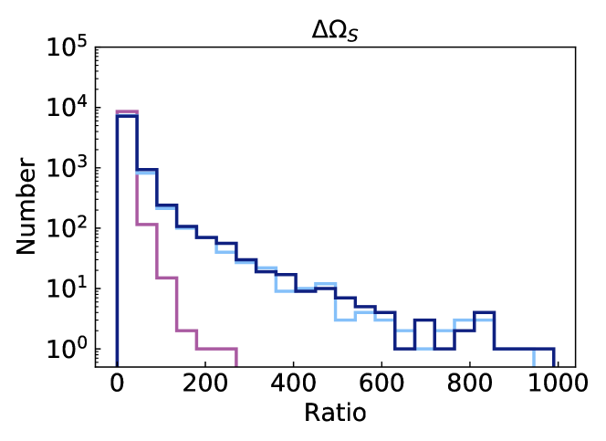
Figure 7: Histograms showing improvement of parameter estimation uncertainties with repect to TianQin (TQ). The horizontal axis shows the ratio of parameter uncertainties between TQ and the corresponding network, the larger value represents better improvement.

IV.4 The estimation of the merger rate

In this section, we estimate the number of DWD mergers that can be expected for TianQin. DWDs typically merge in the frequency ranging from decihertz to a few hertz. Therefore, the inspiral GW signals can be detected by TianQin.

We consider a DWD with equal mass components of 1M_⊙, so that the total mass of the binary is larger the Chandrasekhar mass limit. We model its chirping signal with the IMRPhenomPv2 waveform Hannam et al. (2014) and calculate SNR using Eq. (16). Following Wang et al. (2019) and assuming a mission lifetime of 5 years for TianQin, we find that the SNR of our example DWD binary is

$$\rho\approx 20\left(\frac{{\rm 1~{}Mpc}}{d}\right)\,.$$ (26)

This result implies that TianQin can detect SNe Ia explosions within the virial radius of the Local Group.

The SNe Ia rate in the Milky Way is 0.01-0.005/yr Hallakoun and Maoz (2019), and the DWD merger rate is 4.5-7 times the SNe Ia rate (as most DWDs would not exceed the Chandrasekhar limit) Maoz et al. (2018); Wang and Liu (2020). This means that an optimistic estimation of the DWD merger rate is $\sim$0.07/yr in the Galaxy.

To estimate the DWD merger rate in the Local Group, we note that the Local Group is consists of about 60 galaxies, most with masses $<10^{8}$M_⊙. Therefore, the total mass of the Local Group galaxies is dominated by the Milky Way and the Andromeda Galaxy Karachentsev and Kashibadze (2006). The masses of the Milky Way and the Andromeda Galaxy are $0.8-1.5\times 10^{12}\,\mathrm{M}_{\odot}$ and $1\sim 2\times 10^{12}\,\mathrm{M}_{\odot}$ Karachentsev and Kashibadze (2006), respectively. Assuming that the DWD merger rate is proportional to the galaxy mass, one can obtain that the DWD merger rate within the Local Group ranges from 0.0375/yr to 0.25/yr, using the relation

$$R_{\mathrm{total}}\Big{(}1+\frac{M_{31}}{M_{\mathrm{MW}}}\Big{)}\times R_{\mathrm{MW}},$$ (27)

where $M_{31}$ and $M_{\mathrm{MW}}$ are masses of Andromeda Galaxy and Milky Way, and $R_{\mathrm{MW}}$ is the DWD merger rate in our Galaxy. Therefore, in the optimistic case, TianQin would be able to observe one DWD merger event with its lifetime of 5 years.

V Summary and discussion

In this paper, we carried out the first prediction for the detection of Galactic DWDs with TianQin. For this purpose, we adopted a catalogue of known DWDs discovered with EM observations and a mock Galactic population constructed using a binary population synthesis method. We outlined analytical expressions and numerical methods for computing noise curves, SNR, and uncertainties on the measured parameters of monochromatic GW sources for the TianQin mission with fixed orientation. By considering different detector orientations, in this work we also addressed an interesting open question regarding the optimal orientation of the mission.

First, we assessed the strength of the foreground arising from unresolved Galactic DWDs. We found that its effect can be largely ignored for the present design sensitivity of the TianQin detector.

When considering the sample of known DWDs, we found that out of 81 CVBs with orbital periods $\lesssim 5$ hour, TianQin can detect 12 with SNR $\geq 5$ within 5 years of mission lifetime. In particular, we found that TianQin will be able to detect J0806 (its main verification source) already after two days of observations. We estimated that the expected uncertainty on GW amplitude for verification binaries is within a few per cent. For verification binaries with small inclination angles (nearly face-on), this uncertainty can be improved by up to a factor of 16, if the binary inclination angle is known a priori.

When analyzing a synthetic Galactic population of DWD, we found that the overall number of detections is expected to be $8.7\times 10^{3}$ for the full mission duration of 5 years. We found typical value (median) of $\sim 10^{-7}$ on the relative uncertainty of DWDs’ orbital periods, 0.26 on the relative uncertainty of GW amplitude, 0.20 uncertainty on $\cos{\iota}$, and $\sim 1$ deg² uncertainty on sky positions. About 39% can be localized to within better than 1 deg².

Finally, we outlined a proof-of-principle calculation showing that TianQin is expected to detect one DWD merger event with a supernovae type Ia-like counterpart during its five years of operation time.

In addition to TianQin’s nominal orientation (TQ, pointing towards J0806), we also analyzed a variation of the mission oriented perpendicularly (TQ II), and different networks of simultaneously operational GW detectors TQ I+II, TQ + LISA, and TQ I+II + LISA. Although TQ II and TQ I+II can detect the same set of 12 verification binaries as TianQin (TQ), the total number of detections increases by $\sim 1.3$ when considering the network TQ I+II. In addition, the total number of binaries localized to better than 1 deg² also increases to 54% of the total detected sample. We find that the major advantage of combining TianQin and LISA, besides increasing the total number of detections, consists in the improvement on binary parameter uncertainties by $1$-$2$ orders of magnitude, while the improvement the sky localization can reach up to 3 orders of magnitude.

We are living in the era of large astronomical surveys with the number of known DWDs increasing every year thanks to surveys like ELM Brown et al. (2016) and ZTF Bellm (2014). The upcoming LSST LSST Science Collaboration et al. (2009), GOTO Steeghs (2017), and BlackGem Bloemen et al. (2015) will further enlarge the sample by the time TianQin will fly. We show that the TianQin mission has the potential to push the DWD field in the regime of robust statistical studies by increasing the number of detected DWDs to several thousand. By combining data from GW observatories such as TianQin with those from the aforementioned large optical surveys, we will enable multi-messenger studies and advance our knowledge about these unique binary systems.

Appendix A Table of the selected candidate verification binaries

All the selected CVBs are listed in Table LABEL:tb:VB_parameter, with the ecliptic coordinates ($\lambda$, $\beta$); the GW frequency $f=2/P$, with $P$ being the orbital period of the corresponding binary stars; the luminosity distance $d$; the inclination angle $\iota$ of the source; and the heavier and lighter masses, $M$ and $m$, respectively, of the component stars. In some cases, there is no direct measurement on the masses or the inclination angles, so estimated values are assigned based on the evolutionary stage and the mass ratio of the corresponding system. All such values are given within square brackets. We make a conservative choice of 5 kpc for the distance to J0806 Roelofs et al. (2010). The right column of Table LABEL:tb:VB_parameter uses Roman numerals to denote the sources from which the parameters of the listed sources are taken: (i) Kupfer et al. (2018), (ii) Ramsay et al. (2018), (iii) Korol et al. (2017), (iv) Burdge et al. (2019a), (v) Brown et al. (2020), (vi) Burdge et al. (2019b), (vii) Coughlin et al. (2020), (viii) Brown et al. (2016), (ix) Nelemans (2010), and the references therein.

Table 5: The sample of candidate verification binaries. ^a As these systems have no measured parallaxes form Gaia DR2, the distance is estimated by other previously observations.

Source	$\lambda$	$\beta$	$f$	$d$	$M$	$m$	$\iota$	Refs.
	[deg]	[deg]	[mHz]	[kpc]	[$\mathrm{M}_{\odot}$]	[$\mathrm{M}_{\odot}$]	[deg]
$\mathbf{AM\>CVn\>type\>systems}$
J0806	120.4425	-4.7040	6.22	[5]a	0.55	0.27	38	i
V407 Vul	294.9945	46.7829	3.51	1.786	[0.8]	[0.177]	[60]	i
ES Cet	24.6120	-20.3339	3.22	1.584	[0.8]	[0.161]	[60]	i
SDSS J135154.46–064309.0	208.3879	4.4721	2.12	1.317	[0.8]	[0.100]	[60]	i
AM CVn	170.3858	37.4427	1.94	0.299	0.68	0.125	43	i
SDSS J190817.07+394036.4	298.2172	61.4542	1.84	1.044	[0.8]	[0.085]	15	i
HP Lib	235.0882	4.9597	1.81	0.276	0.645	0.068	30	i
PTF1 J191905.19+481506.2	309.0023	69.0290	1.48	1.338	[0.8]	[0.066]	[60]	i
ASASSN-14cc	303.9576	-42.8640	1.48	1.019	[0.6]	[0.01]	[60]	ii
CXOGBS J175107.6–294037	268.0614	-6.2526	1.45	0.971	[0.8]	[0.064]	[60]	i
CR Boo	202.2728	17.8971	1.36	0.337a	0.885	0.066	30	i
KL Dra	334.1334	78.3217	1.33	0.956	0.76	0.057	[60]	ii,iii
V803 Cen	216.1673	-30.3166	1.25	0.347a	0.975	0.084	13.5	i
PTF1 J071912.13+485834.0	104.3883	26.5213	1.24	0.861	[0.8]	[0.053]	[60]	i,ii
SDSS J092638.71+362402.4	132.2867	20.2342	1.18	0.577	0.85	0.035	82.6	ii,iii
CP Eri	42.1327	-26.4276	1.17	0.964	[0.8]	[0.049]	[60]	i,ii
SDSS J104325.08+563258.1	136.2923	43.9158	1.17	0.979	[0.6]	[0.01]	[60]	ii
CRTS J0910-2008	147.3411	-34.5979	1.12	1.113	[0.6]	[0.01]	[60]	ii
CRTS J0105+1903	22.5049	11.1283	1.05	0.734	[0.6]	[0.01]	[60]	ii
V406 Hya/2003aw	140.7336	-21.2342	0.99	0.504	[0.8]	[0.040]	[60]	i,ii
SDSS J173047.59+554518.5	248.6846	78.6529	0.95	0.911	[0.6]	[0.01]	[60]	ii
2QZ J142701.6–012310	214.8878	12.4608	0.91	0.677	[0.6]	[0.015]	[60]	ii,iii
SDSS J124058.03–015919.2	190.1933	2.2262	0.89	0.577	[0.8]	[0.035]	[60]	i,ii
NSV1440	283.1788	-72.6108	0.89	0.377	[0.6]	[0.01]	[60]	ii
SDSS J012940.05+384210.4	35.8760	27.0847	0.89	0.508	[0.8]	[0.034]	[60]	i,ii
SDSS J172102.48+273301.2	256.3525	50.5292	0.87	0.995	[0.6]	[0.01]	[60]	ii
ASASSN-14mv	107.1184	-1.4233	0.82	0.247	[0.6]	[0.01]	[60]	ii
ASASSN-14ei	15.2639	-59.9095	0.78	0.255	[0.6]	[0.01]	[60]	ii
SDSS J152509.57+360054.5	214.3101	52.2364	0.75	0.524	[0.6]	[0.01]	[60]	ii
SDSS J080449.49+161624.8	119.9052	-3.9847	0.75	0.828	[0.8]	[0.027]	[60]	i,ii
SDSS J141118.31+481257.6	183.5559	55.8748	0.72	0.429	[0.6]	[0.01]	[60]	ii
GP Com	187.7210	23.0012	0.72	0.073	0.59	0.011	[60]	ii,iii
SDSS J090221.35+381941.9	126.7527	20.5254	0.69	0.461	[0.6]	[0.01]	[60]	ii
ASASSN-14cn	183.9170	78.0916	0.67	0.259	0.87	0.025	86.3	i,ii
SDSS J120841.96+355025.2	165.8193	33.3289	0.63	0.202	[0.8]	[0.022]	[60]	i,ii
SDSS J164228.06+193410.0	245.3756	41.3659	0.62	1.044	[0.6]	[0.01]	[60]	ii
SDSS J155252.48+320150.9	225.2376	50.6483	0.59	0.443	[0.6]	[0.01]	[60]	ii
SDSS J113732.32+405458.3	156.4126	34.8546	0.56	0.209	[0.6]	[0.01]	[60]	ii
V396 Hya/CE 315	205.7504	-14.4638	0.51	0.094	[0.8]	[0.016]	[60]	i,ii
SDSS J1319+5915	159.2931	59.0926	0.51	0.205	[0.6]	[0.01]	[60]	ii
$\mathbf{detached\>DWD}$
ZTF J153932.16+502738.8	205.0315	66.1616	4.82	1.262	0.61	0.21	84	iv
SDSS J065133.34+284423.4	101.3396	5.8048	2.61	0.933	0.247	0.49	86.9	i
SDSS J093506.92+441107.0	130.9795	28.0912	1.68	0.645a	0.312	0.75	[60]	i
SDSS J232230.20+050942.06	353.4373	8.4572	1.66	0.779	0.24	0.27	27	v
PTF J053332.05+020911.6	82.9097	-21.1234	1.62	1.253	0.65	0.167	72.8	vi
SDSS J010657.39–100003.3	11.4582	-15.7928	0.85	0.758	0.188	0.57	67	i,iii
SDSS J163030.58+423305.7	231.7612	63.0501	0.84	1.019	0.298	0.76	[60]	i
SDSS J082239.54+304857.2	120.6816	11.0965	0.83	0.861	0.304	0.524	88.1	i,iii
ZTF J190125.42+530929.5	306.8131	74.6335	0.82	0.898	0.50	0.20	86.2	vii
SDSS J104336.27+055149.9	160.1545	-2.0480	0.73	1.744	0.183	0.76	[60]	i,iii
SDSS J105353.89+520031.0	141.2200	40.8002	0.54	0.683	0.204	0.75	[60]	i,iii
SDSS J005648.23–061141.5	10.6273	-11.3044	0.53	0.620	0.180	0.82	[60]	i,iii
SDSS J105611.02+653631.5	130.4076	52.2268	0.53	1.104	0.334	0.76	[60]	i,iii
SDSS J092345.59+302805.0	133.7151	14.4268	0.51	0.299	0.275	0.76	[60]	i
SDSS J143633.28+501026.9	187.5011	59.9313	0.50	1.011	0.234	0.78	[60]	i,iii
SDSS J082511.90+115236.4	125.7257	-7.1746	0.40	1.786	0.278	0.80	[60]	i,iii
WD 0957–666	208.5263	-67.3013	0.38	0.163	0.37	0.32	68	i,iii
SDSS J174140.49+652638.7	208.8283	87.8286	0.38	1.159	0.170	1.17	[60]	i,iii
SDSS J075552.40+490627.9	110.9953	27.7583	0.37	2.620a	0.176	0.81	[60]	iii
SDSS J233821.51–205222.8	346.5446	-16.9689	0.30	0.429	0.15	0.263	[60]	iii
SDSS J230919.90+260346.7	359.6100	28.7808	0.30	1.765	0.176	0.96	[60]	viii
SDSS J084910.13+044528.7	133.3917	-12.5404	0.29	1.002	0.176	0.65	[60]	iii
SDSS J002207.65–101423.5	0.9548	-11.5858	0.29	1.151a	0.21	0.375	[60]	iii
SDSS J075141.18–014120.9	120.3746	-22.2324	0.29	1.741	0.97	0.194	[60]	iii
SDSS J211921.96–001825.8	322.1533	14.5725	0.27	1.053	0.74	0.158	[60]	iii
SDSS J123410.36–022802.8	188.8196	1.1194	0.25	0.754	0.09	0.23	[60]	iii
SDSS J100559.10+224932.2	145.4432	10.4254	0.24	0.555	0.36	0.31	88.9	iii
SDSS J115219.99+024814.4	177.1265	1.8106	0.23	0.718	0.47	0.41	89.2	iii
SDSS J105435.78–212155.9	173.8923	-26.0107	0.22	1.313	0.39	0.168	[60]	iii
SDSS J074511.56+194926.5	114.6397	-1.3939	0.20	0.875	0.1	0.156	[60]	iii
WD 1242–105	194.5586	-5.5520	0.19	0.040	0.56	0.39	45.1	i,iii
SDSS J110815.50+151246.6	162.1662	8.9070	0.19	0.698a	0.42	0.167	[60]	iii
WD 1101+364	152.2513	27.6895	0.16	0.088	0.36	0.31	[60]	iii
WD 1704+4807BC	242.3234	70.1865	0.16	0.039	0.39	0.56	[60]	ix
SDSS J011210.25+183503.7	23.7268	10.1149	0.16	0.843	0.62	0.16	[60]	iii
SDSS J123316.20+160204.6	181.0654	17.9826	0.15	1.207	0.169	0.98	[60]	viii
SDSS J113017.42+385549.9	156.0760	32.4474	0.15	0.884	0.72	0.286	[60]	iii
SDSS J111215.82+111745.0	164.6171	5.6844	0.13	0.384	0.14	0.169	[60]	iii
SDSS J100554.05+355014.2	140.4558	22.5307	0.13	1.747	0.168	0.75	[60]	viii
SDSS J144342.74+150938.6	213.1397	29.4368	0.12	0.839	0.84	0.181	[60]	iii
SDSS J184037.78+642312.3	337.4095	85.2636	0.12	0.829	0.65	0.177	[60]	iii

Appendix B SNR OF CANDIDATE VERIFICATION BINARIES

The GW amplitudes and SNR of all selected CVBs are listed in Table LABEL:tb:VB_SNR, assuming a nominal mission lifetime of five years and the three configurations of TianQin, $\phi_{0}=\pi$ and $\psi_{S}=\pi/2$ for all binaries.

Table 6: The expected amplitude $\mathcal{A}$ and SNR of 81 candidate verification binaries. $\mathcal{A}$ is given in units of $10^{-23}$.

Source	$\mathcal{A}$		SNR
		TQ	TQ II	TQ I+II
$\mathbf{AM\>CVn\>type\>systems}$
J0806	6.4	116.202	41.657	123.443
V407 Vul	11.0	41.528	21.537	46.780
ES Cet	10.7	17.775	42.110	45.708
SDSS J135154.46–064309.0	6.2	4.454	11.345	12.188
AM CVn	28.3	31.245	37.499	48.810
SDSS J190817.07+394036.4	6.1	8.622	5.077	10.006
HP Lib	15.7	16.619	29.427	33.795
PTF1 J191905.19+481506.2	3.2	1.526	1.122	1.894
ASASSN-14cc	0.5	0.338	0.188	0.387
CXOGBS J175107.6–294037	4.2	3.022	2.172	3.722
CR Boo	12.9	5.473	14.029	15.058
KL Dra	3.5	1.109	1.006	1.497
V803 Cen	16.0	6.187	15.026	16.249
PTF1 J071912.13+485834.0	3.6	1.844	0.982	2.089
SDSS J092638.71+362402.4	3.6	1.175	0.664	1.350
CP Eri	2.8	0.676	1.384	1.540
SDSS J104325.08+563258.1	0.5	0.178	0.112	0.211
CRTS J0910-2008	0.4	0.164	0.104	0.194
CRTS J0105+1903	0.6	0.108	0.256	0.277
V406 Hya/2003aw	4.0	1.414	0.745	1.599
SDSS J173047.59+554518.5	0.4	0.069	0.066	0.096
2QZ J142701.6–012310	0.9	0.115	0.282	0.304
SDSS J124058.03–015919.2	2.8	0.436	0.842	0.948
NSV1440	1.0	0.140	0.130	0.191
SDSS J012940.05+384210.4	3.1	0.389	0.882	0.964
SDSS J172102.48+273301.2	0.4	0.069	0.063	0.093
ASASSN-14mv	1.5	0.388	0.174	0.425
ASASSN-14ei	1.4	0.133	0.192	0.233
SDSS J152509.57+360054.5	0.7	0.059	0.097	0.114
SDSS J080449.49+161624.8	1.4	0.304	0.119	0.326
SDSS J141118.31+481257.6	0.8	0.068	0.093	0.115
GP Com	5.0	0.490	0.882	1.009
SDSS J090221.35+381941.9	0.7	0.121	0.053	0.132
ASASSN-14cn	4.0	0.220	0.227	0.316
SDSS J120841.96+355025.2	4.1	0.383	0.408	0.560
SDSS J164228.06+193410.0	0.3	0.025	0.029	0.038
SDSS J155252.48+320150.9	0.7	0.039	0.060	0.072
SDSS J113732.32+405458.3	1.4	0.110	0.095	0.145
V396 Hya/CE 315	5.5	0.221	0.535	0.579
SDSS J1319+5915	1.3	0.063	0.062	0.089
$\mathbf{detached\>DWD}$
ZTF J153932.16+502738.8	18.4	51.351	60.184	79.114
SDSS J065133.34+284423.4	16.2	26.535	15.700	30.831
SDSS J093506.92+441107.0	29.9	28.797	14.245	32.128
SDSS J232230.20+050942.06	8.7	9.973	12.371	15.891
PTF J053332.05+020911.6	7.6	4.965	4.042	6.402
SDSS J010657.39–100003.3	8.3	0.989	1.892	2.135
SDSS J163030.58+423305.7	11.6	1.423	1.721	2.233
SDSS J082239.54+304857.2	10.4	1.713	0.887	1.929
ZTF J190125.42+530929.5	6.5	0.614	0.549	0.824
SDSS J104336.27+055149.9	3.9	0.649	0.561	0.857
SDSS J105353.89+520031.0	9.0	0.698	0.457	0.835
SDSS J005648.23–061141.5	9.3	0.475	0.931	1.045
SDSS J105611.02+653631.5	8.7	0.570	0.378	0.684
SDSS J092345.59+302805.0	26.2	2.422	1.138	2.675
SDSS J143633.28+501026.9	6.7	0.262	0.359	0.444
SDSS J082511.90+115236.4	3.9	0.235	0.094	0.253
WD 0957–666	25.7	0.502	0.621	0.798
SDSS J174140.49+652638.7	4.9	0.104	0.103	0.147
SDSS J075552.40+490627.9	1.7	0.072	0.035	0.080
SDSS J233821.51–205222.8	3.3	0.073	0.078	0.107
SDSS J230919.90+260346.7	2.4	0.046	0.062	0.077
SDSS J084910.13+044528.7	3.2	0.094	0.042	0.103
SDSS J002207.65–101423.5	2.1	0.036	0.056	0.067
SDSS J075141.18–014120.9	2.7	0.078	0.032	0.084
SDSS J211921.96–001825.8	2.9	0.069	0.037	0.078
SDSS J123410.36–022802.8	0.9	0.011	0.020	0.022
SDSS J100559.10+224932.2	5.3	0.059	0.039	0.071
SDSS J115219.99+024814.4	6.3	0.047	0.062	0.078
SDSS J105435.78–212155.9	1.3	0.014	0.017	0.022
SDSS J074511.56+194926.5	0.6	0.008	0.003	0.008
WD 1242–105	109.2	0.755	1.656	1.820
SDSS J110815.50+151246.6	2.4	0.022	0.020	0.030
WD 1101+364	25.4	0.159	0.120	0.199
WD 1704+4807BC	99.9	0.376	0.388	0.541
SDSS J011210.25+183503.7	2.2	0.008	0.019	0.020
SDSS J123316.20+160204.6	2.2	0.009	0.014	0.016
SDSS J113017.42+385549.9	3.9	0.019	0.016	0.026
SDSS J111215.82+111745.0	1.4	0.005	0.005	0.008
SDSS J100554.05+355014.2	1.1	0.005	0.003	0.006
SDSS J144342.74+150938.6	2.6	0.005	0.010	0.011
SDSS J184037.78+642312.3	2.1	0.004	0.004	0.005

Appendix C Re-expression of the responsed Gravitational Wave Signal

For convenience of calculation, we rearrange the expression for the waveform in the detector:

$$h(t)=A(t)\cos\Psi(t)\,,$$ (28)

where the waveform amplitude $A(t)$ is

$$A(t)=\left[(A_{+}F^{+}(t))^{2}+(A_{\times}F^{\times}(t))^{2}\right]^{1/2}.$$ (29)

$A_{+}$ and $A_{\times}$ are given by

$$A_{+}=\mathcal{A}(1+\cos\iota^{2}),\quad A_{\times}=2\mathcal{A}\cos\iota.$$ (30)

The phase of the waveform is

$$\Psi(t)=2\pi ft+\phi_{0}+\Phi_{D}(t)+\Phi_{P}(t),$$ (31)

The polarization phase $\Phi_{P}(t)$ is given by

$$\Phi_{P}(t)=\tan^{-1}\left(\frac{-A_{\times}F^{\times}(t)}{A_{+}F^{+}(t)}\right)\,.$$ (32)

Appendix D Derivation of the average amplitude

In order to verify our SNR calculation, more specifically the calculation of average amplitude, we can obtain the average amplitude from the antenna beam patterns function given by Eq. (13) in Hu et al. (2018):

$$F^{+}(t,\theta,\phi,\psi) = \cos 2\psi\xi^{+}(t;\theta,\phi)-sin2\psi\xi^{\times}(t;\theta,\phi)\,,$$

$$F^{\times}(t,\theta,\phi,\psi) = \sin 2\psi\xi^{+}(t;\theta,\phi)+\cos 2\psi\xi^{\times}(t;\theta,\phi)\,,$$ (33)

and

$$\xi^{+}(t;\theta,\phi) = \frac{\sqrt{3}}{32}(4\cos 2(\kappa-\beta^{\prime})((3+\cos 2\theta)\sin\theta_{s}\sin 2(\phi-\phi_{s})+2\sin(\phi-\phi_{s})\sin 2\theta\cos\theta_{s})$$

$$-\sin 2(\kappa-\beta^{\prime})(3+\cos 2(\phi-\phi_{s})(9+\cos 2\theta(3-\cos 2\theta_{s}))+6\cos 2\theta_{s}\sin^{2}(\phi-\phi_{s})$$

$$-6\cos 2\theta\cos^{2}\theta_{s}+4\cos(\phi-\phi_{s})\sin 2\theta\sin 2\theta_{s}))\,,$$

$$\xi^{\times}(t;\theta,\phi) = \frac{\sqrt{3}}{8}(-4\cos 2(\kappa-\beta^{\prime})(\cos 2(\phi-\phi_{s})\cos\theta\sin\theta_{s}+\cos(\phi-\phi_{s})\sin\theta\cos\theta_{s})$$ (34)

$$+\sin 2(\kappa-\beta^{\prime})(\cos\theta(3-\cos 2\theta_{s})\sin 2(\phi_{s}-\phi)+2\sin(\phi_{s}-\phi)\sin\theta\sin 2\theta_{s}))\,.$$

where $\kappa=2\pi f_{sc}t+\lambda^{\prime}$, $f_{sc}\approx 1/(3.65d)$ is the modulation frequency from the rotation of the satellites around the guiding center. $\lambda^{\prime}$ and $\beta^{\prime}$ are some of initial phase of constant.

In the above expression, $\theta=\pi/2-\beta$ and $\phi=\lambda$ are the source location in the ecliptic coordinate system. $\psi$ is the polarization angle. $\theta_{s}$ and $\phi_{s}$ are the ecliptic coordinates of the reference source. For the reference source of TianQin is J0806, $\theta_{s}=-4.7040^{\circ}$ and $\phi_{s}=120.4425^{\circ}$.

By performing the same process as described in Section III.4, we get some expressions similar to Eqs. (19)-(21), given below:

$$\langle A^{2}\rangle = \mathcal{A}^{2}\left[(1+\cos^{2}\iota)^{2}\langle F_{+}^{2}\rangle+4\cos^{2}\iota\langle F_{\times}^{2}\rangle\right]\,,$$ (35)

$$\langle F_{+}^{2}\rangle = \frac{1}{4}(\cos^{2}2\psi\langle D^{2}_{+}\rangle-\sin 4\psi\langle D_{+}D_{\times}\rangle+\sin^{2}2\psi\langle D^{2}_{\times}\rangle)\,,$$ (36)

$$\langle F_{\times}^{2}\rangle = \frac{1}{4}(\cos^{2}2\psi\langle D^{2}_{\times}\rangle+\sin 4\psi\langle D_{+}D_{\times}\rangle+\sin^{2}2\psi\langle D^{2}_{+}\rangle)\,.$$ (37)

where

$$\langle D^{2}_{+}\rangle = b^{2}_{1}+b^{2}_{2}\,,$$

$$\langle D^{2}_{\times}\rangle = b^{2}_{3}+b^{2}_{4}\,,$$

$$\langle D_{+}D_{\times}\rangle = -2(b_{1}b_{3}+b_{2}b_{4})\,,$$ (38)

and

$$b_{1} = \frac{\sqrt{3}}{8}((3+\cos 2\theta)\sin\theta_{s}\sin 2(\phi-\phi_{s})+2\sin(\phi-\phi_{s})\sin 2\theta\cos\theta_{s})\,,$$

$$b_{2} = \frac{\sqrt{3}}{32}(3+\cos 2(\phi-\phi_{s})(9+\cos 2\theta(3-\cos 2\theta_{s}))+6\cos 2\theta_{s}\sin^{2}(\phi-\phi_{s})$$

$$-6\cos 2\theta\cos^{2}\theta_{s}+4\cos(\phi-\phi_{s})\sin 2\theta\sin 2\theta_{s})\,,$$

$$b_{3} = \frac{\sqrt{3}}{2}(\cos 2(\phi-\phi_{s})\cos\theta\sin\theta_{s}+\cos(\phi-\phi_{s})\sin\theta\cos\theta_{s})\,,$$

$$b_{4} = \frac{\sqrt{3}}{8}((3-\cos 2\theta_{s})\cos\theta\sin 2(\phi_{s}-\phi)+2\sin(\phi_{s}-\phi)\sin\theta\sin 2\theta_{s})\,.$$ (39)

The average amplitude calculated by Eqs. (35)-(39) is consistent with Eqs. (19)-(21), with $0.1\%\sim 1\%$ of relative uncertainty.

Appendix E Coordinate transformation

The transformation of the source position from the ecliptic coordinates ($\beta,\lambda$) to the detector coordinates ($\theta_{S},\phi_{S}$) and ($\theta_{S}^{\prime},\phi_{S}^{\prime}$) of the TianQin (TQ) and TQ II is described by the following formula:

$$\left(\begin{array}[]{c}d\sin\theta_{S}\cos\phi_{S}\\ d\sin\theta_{S}\sin\phi_{S}\\ d\cos\theta_{S}\\ \end{array}\right)=R_{x}(\theta=120^{\circ}-90^{\circ})R_{z}(\theta=-4.7^{\circ}-90^{\circ})\left(\begin{array}[]{c}d\cos\beta\cos\lambda\\ d\cos\beta\sin\lambda\\ d\sin\beta\\ \end{array}\right)$$ (40)

$${\rm and}~{}\left(\begin{array}[]{c}d\sin\theta_{S}^{\prime}\cos\phi_{S}^{\prime}\\ d\sin\theta_{S}^{\prime}\sin\phi_{S}^{\prime}\\ d\cos\theta_{S}^{\prime}\\ \end{array}\right)=R_{y}(\theta=90^{\circ})R_{x}(\theta=120^{\circ}-90^{\circ})R_{z}(\theta=-4.7^{\circ}-90^{\circ})\left(\begin{array}[]{c}d\cos\beta\cos\lambda\\ d\cos\beta\sin\lambda\\ d\sin\beta\\ \end{array}\right),$$ (41)

where the rotation matrices are

$$R_{x}(\theta)=\left(\begin{array}[]{ccc}1&0&0\\ 0&\cos\theta&\sin\theta\\ 0&-\sin\theta&\cos\theta\\ \end{array}\right),R_{y}(\theta)=\left(\begin{array}[]{ccc}\cos\theta&0&-\sin\theta\\ 0&1&0\\ \sin\theta&0&\cos\theta\\ \end{array}\right){\rm,and}~{}R_{z}(\theta)=\left(\begin{array}[]{ccc}\cos\theta&\sin\theta&0\\ -\sin\theta&\cos\theta&0\\ 0&0&1\\ \end{array}\right).$$ (42)

References

- Abbott et al. (2016a) B. P. Abbott et al. (LIGO Scientific Collaboration and Virgo Collaboration), Phys. Rev. Lett. 116, 061102 (2016a).
- Einstein (1916) A. Einstein, Sitzungsberichte der Königlich Preußischen Akademie der Wissenschaften (Berlin , 688 (1916).
- Abbott et al. (2016b) B. P. Abbott et al. (LIGO Scientific Collaboration and Virgo Collaboration), Phys. Rev. X 6, 041015 (2016b).
- Abbott et al. (2019) B. P. Abbott et al. (LIGO Scientific Collaboration and Virgo Collaboration), Phys. Rev. X 9, 031040 (2019).
- The LIGO Scientific Collaboration et al. (2020) The LIGO Scientific Collaboration, the Virgo Collaboration, et al., arXiv e-prints , arXiv:2004.08342 (2020), arXiv:2004.08342 [astro-ph.HE] .
- Abbott et al. (2020a) B. P. Abbott et al., Astrophysical Journal 892, L3 (2020a), arXiv:2001.01761 [astro-ph.HE] .
- Abbott et al. (2020b) R. Abbott et al., Astrophysical Journal 896, L44 (2020b), arXiv:2006.12611 [astro-ph.HE] .
- McWilliams et al. (2019) S. T. McWilliams, R. Caldwell, K. Holley-Bockelmann, S. L. Larson, and M. Vallisneri, arXiv e-prints (2019), arXiv:1903.04592 [astro-ph.HE] .
- Kamionkowski and Kovetz (2016) M. Kamionkowski and E. D. Kovetz, ARA&A 54, 227 (2016), arXiv:1510.06042 .
- Arzoumanian et al. (2018) Z. Arzoumanian et al., Astrophysical Journal 859, 47 (2018), arXiv:1801.02617 [astro-ph.HE] .
- Shannon et al. (2015) R. M. Shannon et al., Science 349, 1522 (2015), arXiv:1509.07320 .
- Amaro-Seoane et al. (2017) P. Amaro-Seoane et al., arXiv e-prints (2017), arXiv:1702.00786 [astro-ph.IM] .
- Luo et al. (2016) J. Luo et al. (TianQin), Class. Quant. Grav. 33, 035010 (2016), arXiv:1512.02076 [astro-ph.IM] .
- Klein et al. (2016) A. Klein, E. Barausse, A. Sesana, A. Petiteau, E. Berti, S. Babak, J. Gair, S. Aoudia, I. Hinder, F. Ohme, and B. Wardell, Phys. Rev. D 93, 024003 (2016).
- Wang et al. (2019) H.-T. Wang, Z. Jiang, A. Sesana, E. Barausse, S.-J. Huang, Y.-F. Wang, W.-F. Feng, Y. Wang, Y.-M. Hu, J. Mei, and J. Luo, Phys. Rev. D 100, 043003 (2019), arXiv:1902.04423 [astro-ph.HE] .
- Magorrian et al. (1998) J. Magorrian, S. Tremaine, D. Richstone, R. Bender, G. Bower, A. Dressler, S. M. Faber, K. Gebhardt, R. Green, C. Grillmair, J. Kormendy, and T. Lauer, Astronomical Journal 115, 2285 (1998), astro-ph/9708072 .
- Lynden-Bell (1969) D. Lynden-Bell, Nature 223, 690 (1969).
- Feng et al. (2019) W.-F. Feng, H.-T. Wang, X.-C. Hu, Y.-M. Hu, and Y. Wang, Phys. Rev. D 99, 123002 (2019), arXiv:1901.02159 [astro-ph.IM] .
- Babak et al. (2017) S. Babak, J. Gair, A. Sesana, E. Barausse, C. F. Sopuerta, C. P. L. Berry, E. Berti, P. Amaro-Seoane, A. Petiteau, and A. Klein, Phys. Rev. D 95, 103012 (2017).
- Fan et al. (2020) H.-M. Fan, Y.-M. Hu, E. Barausse, A. Sesana, J.-D. Zhang, X. Zhang, T.-G. Zi, and J. Mei, arXiv e-prints , arXiv:2005.08212 (2020), arXiv:2005.08212 [astro-ph.HE] .
- Lamberts et al. (2018) A. Lamberts, S. Garrison-Kimmel, P. F. Hopkins, E. Quataert, J. S. Bullock, C. A. Faucher-Giguère, A. Wetzel, D. Kereš, K. Drango, and R. E. Sand erson, MNRAS 480, 2704 (2018), arXiv:1801.03099 [astro-ph.GA] .
- Lau et al. (2020) M. Y. M. Lau, I. Mandel, A. Vigna-Gómez, C. J. Neijssel, S. Stevenson, and A. Sesana, MNRAS 492, 3061 (2020), arXiv:1910.12422 [astro-ph.HE] .
- Korol et al. (2017) V. Korol, E. M. Rossi, P. J. Groot, G. Nelemans, S. Toonen, and A. G. A. Brown, MNRAS 470, 1894 (2017), arXiv:1703.02555 [astro-ph.HE] .
- Robson et al. (2018) T. Robson, N. J. Cornish, N. Tamanini, and S. Toonen, Phys. Rev. D 98, 064012 (2018), arXiv:1806.00500 [gr-qc] .
- Romano and Cornish (2017) J. D. Romano and N. J. Cornish, Living Reviews in Relativity 20, 2 (2017), arXiv:1608.06889 [gr-qc] .
- Liang et al. (2020) Z. C. Liang et al., “Science with the tianqin observatory: Preliminary results on stochastic gravitational wave background,” (2020), in prep.
- Korol et al. (2018) V. Korol, O. Koop, and E. M. Rossi, Astrophysical Journal 866, L20 (2018), arXiv:1808.05959 [astro-ph.HE] .
- Berti et al. (2005) E. Berti, A. Buonanno, and C. M. Will, Phys. Rev. D 71, 084025 (2005), gr-qc/0411129 .
- Shi et al. (2019) C. Shi, J. Bao, H. Wang, J.-d. Zhang, Y. Hu, A. Sesana, E. Barausse, J. Mei, and J. Luo, Phys. Rev. D 100, 044036 (2019), arXiv:1902.08922 [gr-qc] .
- Bao et al. (2019) J. Bao, C. Shi, H. Wang, J.-d. Zhang, Y. Hu, J. Mei, and J. Luo, Phys. Rev. D 100, 084024 (2019), arXiv:1905.11674 [gr-qc] .
- Tamanini and Danielski (2018) N. Tamanini and C. Danielski, arXiv e-prints (2018), arXiv:1812.04330 [astro-ph.EP] .
- Nelemans et al. (2001a) G. Nelemans, L. R. Yungelson, and S. F. Portegies Zwart, A&A 375, 890 (2001a), astro-ph/0105221 .
- Yu and Jeffery (2010) S. Yu and C. S. Jeffery, A&A 521, A85 (2010), arXiv:1007.4267 [astro-ph.SR] .
- Breivik et al. (2019) K. Breivik, S. C. Coughlin, M. Zevin, C. L. Rodriguez, K. Kremer, C. S. Ye, J. J. Andrews, M. Kurkowski, M. C. Digman, S. L. Larson, and F. A. Rasio, arXiv e-prints , arXiv:1911.00903 (2019), arXiv:1911.00903 [astro-ph.HE] .
- Postnov and Yungelson (2014) K. A. Postnov and L. R. Yungelson, Living Reviews in Relativity 17, 3 (2014).
- Belczynski et al. (2002) K. Belczynski, V. Kalogera, and T. Bulik, The Astrophysical Journal 572, 407 (2002).
- Nelemans et al. (2001b) G. Nelemans, L. R. Yungelson, S. F. Portegies Zwart, and F. Verbunt, A&A 365, 491 (2001b), astro-ph/0010457 .
- Marsh et al. (2004) T. R. Marsh, G. Nelemans, and D. Steeghs, MNRAS 350, 113 (2004), astro-ph/0312577 .
- Solheim (2010) J.-E. Solheim, PASP 122, 1133 (2010).
- Tauris (2018) T. M. Tauris, Phys. Rev. Lett 121, 131105 (2018), arXiv:1809.03504 [astro-ph.SR] .
- Bildsten et al. (2007) L. Bildsten, K. J. Shen, N. N. Weinberg, and G. Nelemans, APJL 662, L95 (2007), astro-ph/0703578 .
- Webbink (1984) R. F. Webbink, APJ 277, 355 (1984).
- Iben and Tutukov (1984) I. Iben, Jr. and A. V. Tutukov, APJS 54, 335 (1984).
- Piro (2011) A. L. Piro, APJL 740, L53 (2011), arXiv:1108.3110 [astro-ph.SR] .
- Fuller and Lai (2012) J. Fuller and D. Lai, APJL 756, L17 (2012), arXiv:1206.0470 [astro-ph.SR] .
- Dall’Osso and Rossi (2014) S. Dall’Osso and E. M. Rossi, MNRAS 443, 1057 (2014), arXiv:1308.1664 [astro-ph.HE] .
- Mckernan and Ford (2016) B. Mckernan and K. E. S. Ford, Monthly Notices of the Royal Astronomical Society 463, 2039 (2016).
- Littenberg and Yunes (2019) T. B. Littenberg and N. Yunes, Classical and Quantum Gravity 36, 095017 (2019), arXiv:1811.01093 [gr-qc] .
- Cooray and Seto (2004) A. Cooray and N. Seto, Phys. Rev. D 69, 103502 (2004), astro-ph/0311054 .
- Benacquista and Holley-Bockelmann (2006) M. Benacquista and K. Holley-Bockelmann, APJ 645, 589 (2006), astro-ph/0504135 .
- Adams et al. (2012) M. R. Adams, N. J. Cornish, and T. B. Littenberg, Phys. Rev. D 86, 124032 (2012), arXiv:1209.6286 [gr-qc] .
- Korol et al. (2019) V. Korol, E. M. Rossi, and E. Barausse, MNRAS 483, 5518 (2019), arXiv:1806.03306 .
- Wilhelm et al. (2020) M. J. C. Wilhelm, V. Korol, E. M. Rossi, and E. D’Onghia, arXiv e-prints , arXiv:2003.11074 (2020), arXiv:2003.11074 [astro-ph.GA] .
- Steffen et al. (2018) J. H. Steffen, D.-H. Wu, and S. L. Larson, arXiv e-prints (2018), arXiv:1812.03438 [astro-ph.EP] .
- Danielski et al. (2019) C. Danielski, V. Korol, N. Tamanini, and E. M. Rossi, A&A 632, A113 (2019), arXiv:1910.05414 [astro-ph.EP] .
- Yiming Hu (2019) J. L. Yiming Hu, Jianwei Mei, Chinese Science Bulletin , (2019).
- Ye et al. (2019) B.-B. Ye, X. Zhang, M.-Y. Zhou, Y. Wang, H.-M. Yuan, D. Gu, Y. Ding, J. Zhang, J. Mei, and J. Luo, International Journal of Modern Physics D (2019).
- Hu et al. (2017) Y. M. Hu, J. Mei, and J. Luo, National Science Review 4, 683 (2017).
- Hu et al. (2018) X.-C. Hu, X.-H. Li, Y. Wang, W.-F. Feng, M.-Y. Zhou, Y.-M. Hu, S.-C. Hu, J.-W. Mei, and C.-G. Shao, Classical and Quantum Gravity 35, 095008 (2018), arXiv:1803.03368 [gr-qc] .
- Liu et al. (2020) S. Liu, Y.-M. Hu, J.-d. Zhang, and J. Mei, Phys. Rev. D 101, 103027 (2020), arXiv:2004.14242 [astro-ph.HE] .
- Xie et al. (2020) N. Xie et al., “Detecting extra polarization of GW with TianQin,” (2020), in prep.
- Liang et al. (2019) D. Liang, Y. Gong, A. J. Weinstein, C. Zhang, and C. Zhang, Phys. Rev. D 99, 104027 (2019), arXiv:1901.09624 [gr-qc] .
- Zhang et al. (2020) C. Zhang, Q. Gao, Y. Gong, B. Wang, A. J. Weinstein, and C. Zhang, arXiv e-prints , arXiv:2003.01441 (2020), arXiv:2003.01441 [gr-qc] .
- Korol et al. (2020) V. Korol, S. Toonen, A. Klein, V. Belokurov, F. Vincenzo, R. Buscicchio, D. Gerosa, C. J. Moore, E. Roebber, E. M. Rossi, and A. Vecchio, arXiv e-prints , arXiv:2002.10462 (2020), arXiv:2002.10462 [astro-ph.GA] .
- Roebber et al. (2020) E. Roebber, R. Buscicchio, A. Vecchio, C. J. Moore, A. Klein, V. Korol, S. Toonen, D. Gerosa, J. Goldstein, S. M. Gaebel, and T. E. Woods, arXiv e-prints , arXiv:2002.10465 (2020), arXiv:2002.10465 [astro-ph.GA] .
- Nelemans et al. (2004) G. Nelemans, L. R. Yungelson, and S. F. Portegies Zwart, MNRAS 349, 181 (2004), astro-ph/0312193 .
- Nissanke et al. (2012) S. Nissanke, M. Vallisneri, G. Nelemans, and T. A. Prince, Astrophysical Journal 758, 131 (2012), arXiv:1201.4613 .
- Brown et al. (2017) W. R. Brown, M. Kilic, A. Kosakowski, and A. Gianninas, The Astrophysical Journal 847, 10 (2017).
- Maoz et al. (2018) D. Maoz, N. Hallakoun, and C. Badenes, MNRAS 476, 2584 (2018), arXiv:1801.04275 [astro-ph.SR] .
- Ramsay et al. (2018) G. Ramsay, M. J. Green, T. R. Marsh, T. Kupfer, E. Breedt, V. Korol, P. J. Groot, C. Knigge, G. Nelemans, D. Steeghs, P. Woudt, and A. Aungwerojwit, A&A 620, A141 (2018), arXiv:1810.06548 [astro-ph.SR] .
- Burdge et al. (2019a) K. B. Burdge, M. W. Coughlin, J. Fuller, T. Kupfer, E. C. Bellm, L. Bildsten, M. J. Graham, D. L. Kaplan, J. v. Roestel, R. G. Dekany, D. A. Duev, M. Feeney, M. Giomi, G. Helou, S. Kaye, R. R. Laher, A. A. Mahabal, F. J. Masci, R. Riddle, D. L. Shupe, M. T. Soumagnac, R. M. Smith, P. Szkody, R. Walters, S. R. Kulkarni, and T. A. Prince, Nature 571, 528 (2019a), arXiv:1907.11291 [astro-ph.SR] .
- Burdge et al. (2019b) K. B. Burdge, J. Fuller, E. S. Phinney, J. van Roestel, A. Claret, E. Cukanovaite, N. P. Gentile Fusillo, M. W. Coughlin, D. L. Kaplan, T. Kupfer, P.-E. Tremblay, R. G. Dekany, D. A. Duev, M. Feeney, R. Riddle, S. R. Kulkarni, and T. A. Prince, Astrophysical Journal 886, L12 (2019b), arXiv:1910.11389 [astro-ph.SR] .
- Coughlin et al. (2020) M. W. Coughlin, K. Burdge, E. Sterl Phinney, J. van Roestel, E. C. Bellm, R. G. Dekany, A. Delacroix, D. A. Duev, M. Feeney, M. J. Graham, S. R. Kulkarni, T. Kupfer, R. R. Laher, F. J. Masci, T. A. Prince, R. Riddle, P. Rosnet, R. Smith, E. Serabyn, and R. Walters, MNRAS 494, L91 (2020), arXiv:2004.00456 [astro-ph.HE] .
- Brown et al. (2020) W. R. Brown, M. Kilic, A. Bedard, A. Kosakowski, and P. Bergeron, arXiv e-prints , arXiv:2004.00641 (2020), arXiv:2004.00641 [astro-ph.SR] .
- Stroeer and Vecchio (2006) A. Stroeer and A. Vecchio, Classical and Quantum Gravity 23, S809 (2006), arXiv:astro-ph/0605227 [astro-ph] .
- Kupfer et al. (2018) T. Kupfer, S. Shah, G. Nelemans, T. R. Marsh, G. Ramsay, P. J. Groot, D. T. H. Steeghs, and E. M. Rossi, MNRAS 480, 302 (2018).
- Gaia Collaboration et al. (2018) Gaia Collaboration, A. G. A. Brown, A. Vallenari, T. Prusti, J. H. J. de Bruijne, C. Babusiaux, and C. A. L. Bailer-Jones, ArXiv e-prints (2018), arXiv:1804.09365 .
- Strohmayer (2005) T. E. Strohmayer, Astrophysical Journal 627, 920 (2005), arXiv:astro-ph/0504150 [astro-ph] .
- Roelofs et al. (2010) G. H. A. Roelofs, A. Rau, T. R. Marsh, D. Steeghs, P. J. Groot, and G. Nelemans, Astrophysical Journal 711, L138 (2010), arXiv:1003.0658 [astro-ph.SR] .
- Toonen et al. (2012) S. Toonen, G. Nelemans, and S. Portegies Zwart, A&A 546, A70 (2012), arXiv:1208.6446 [astro-ph.HE] .
- Toonen et al. (2017) S. Toonen, M. Hollands, B. T. Gänsicke, and T. Boekholt, A&A 602, A16 (2017), arXiv:1703.06893 [astro-ph.SR] .
- Portegies Zwart and Verbunt (1996) S. F. Portegies Zwart and F. Verbunt, A&A 309, 179 (1996).
- Kroupa et al. (1993) P. Kroupa, C. A. Tout, and G. Gilmore, MNRAS 262, 545 (1993).
- Duchêne and Kraus (2013) G. Duchêne and A. Kraus, ARA&A 51, 269 (2013), arXiv:1303.3028 [astro-ph.SR] .
- Abt (1983) H. A. Abt, ARA&A 21, 343 (1983).
- Heggie (1975) D. C. Heggie, MNRAS 173, 729 (1975).
- Nelemans et al. (2000) G. Nelemans, F. Verbunt, L. R. Yungelson, and S. F. Portegies Zwart, A&A 360, 1011 (2000), astro-ph/0006216 .
- Boissier and Prantzos (1999) S. Boissier and N. Prantzos, MNRAS 307, 857 (1999), astro-ph/9902148 .
- Landau and Lifshitz (1962) L. D. Landau and E. M. Lifshitz, The classical theory of fields; 2nd ed., Course of theoretical physics (Pergamon, London, 1962) trans. from the Russian.
- Peters and Mathews (1963) P. C. Peters and J. Mathews, Phys. Rev. 131, 435 (1963).
- Cutler (1998) C. Cutler, Phys. Rev. D 57, 7089 (1998).
- Cornish and Rubbo (2003) N. J. Cornish and L. J. Rubbo, Phys. Rev. D 67, 029905 (2003), arXiv:gr-qc/0209011 [gr-qc] .
- Robson et al. (2019) T. Robson, N. J. Cornish, and C. Liu, Classical and Quantum Gravity 36, 105011 (2019), arXiv:1803.01944 [astro-ph.HE] .
- Finn (1992) L. S. Finn, Phys. Rev. D 46, 5236 (1992).
- Cutler and Flanagan (1994) C. Cutler and E. E. Flanagan, Phys. Rev. D 49, 2658 (1994).
- Cornish and Robson (2017) N. Cornish and T. Robson, Proceedings, 11th International LISA Symposium: Zurich, Switzerland, September 5-9, 2016, J. Phys. Conf. Ser. 840, 012024 (2017), arXiv:1703.09858 [astro-ph.IM] .
- Littenberg and Cornish (2015) T. B. Littenberg and N. J. Cornish, Phys. Rev. D91, 084034 (2015), arXiv:1410.3852 [gr-qc] .
- Shah et al. (2012) S. Shah, M. van der Sluys, and G. Nelemans, A&A 544, A153 (2012), arXiv:1207.6770 [astro-ph.IM] .
- Littenberg et al. (2013) T. B. Littenberg, S. L. Larson, G. Nelemans, and N. J. Cornish, MNRAS 429, 2361 (2013).
- Hannam et al. (2014) M. Hannam, P. Schmidt, A. Bohé, L. Haegel, S. Husa, F. Ohme, G. Pratten, and M. Pürrer, Phys. Rev. Lett 113, 151101 (2014), arXiv:1308.3271 [gr-qc] .
- Hallakoun and Maoz (2019) N. Hallakoun and D. Maoz, arXiv e-prints (2019), arXiv:1905.00032 [astro-ph.SR] .
- Wang and Liu (2020) B. Wang and D. Liu, arXiv e-prints , arXiv:2005.01880 (2020), arXiv:2005.01880 [astro-ph.SR] .
- Karachentsev and Kashibadze (2006) I. D. Karachentsev and O. G. Kashibadze, Astrophysics 49, 3 (2006).
- Brown et al. (2016) W. R. Brown, M. Kilic, S. J. Kenyon, and A. Gianninas, Astrophysical Journal 824, 46 (2016), arXiv:1604.04269 [astro-ph.SR] .
- Bellm (2014) E. Bellm, in The Third Hot-wiring the Transient Universe Workshop, edited by P. R. Wozniak, M. J. Graham, A. A. Mahabal, and R. Seaman (2014) pp. 27–33, arXiv:1410.8185 [astro-ph.IM] .
- LSST Science Collaboration et al. (2009) LSST Science Collaboration, P. A. Abell, J. Allison, S. F. Anderson, J. R. Andrew, J. R. P. Angel, L. Armus, D. Arnett, S. J. Asztalos, T. S. Axelrod, and et al., arXiv e-prints (2009), arXiv:0912.0201 [astro-ph.IM] .
- Steeghs (2017) D. Steeghs, Nature Astronomy 1, 741 (2017).
- Bloemen et al. (2015) S. Bloemen, P. Groot, G. Nelemans, and M. Klein-Wolt, “The BlackGEM Array: Searching for Gravitational Wave Source Counterparts to Study Ultra-Compact Binaries,” in Living Together: Planets, Host Stars and Binaries, Astronomical Society of the Pacific Conference Series, Vol. 496, edited by S. M. Rucinski, G. Torres, and M. Zejda (2015) p. 254.
- Nelemans (2010) G. Nelemans, LISA Verification Binaries (2010).