Topology Inference with Multivariate Cumulants:
The Möbius Inference Algorithm

Abstract

Many tasks regarding the monitoring, management, and design of communication networks rely on knowledge of the routing topology. However, the standard approach to topology mapping—namely, active probing with traceroutes—relies on cooperation from increasingly non-cooperative routers, leading to missing information. Network tomography, which uses end-to-end measurements of additive link metrics (like delays or log packet loss rates) across monitor paths, is a possible remedy. Network tomography does not require that routers cooperate with traceroute probes, and it has already been used to infer the structure of multicast trees. This paper goes a step further. We provide a tomographic method to infer the underlying routing topology of an arbitrary set of monitor paths using the joint distribution of end-to-end measurements, without making any assumptions on routing behavior. Our approach, called the Möbius Inference Algorithm (MIA), uses cumulants of this distribution to quantify high-order interactions among monitor paths, and it applies Möbius inversion to “disentangle” these interactions. In addition to MIA, we provide a more practical variant called Sparse Möbius Inference, which uses various sparsity heuristics to reduce the number and order of cumulants required to be estimated. We show the viability of our approach using synthetic case studies based on real-world ISP topologies.

I Introduction

Many tasks regarding the monitoring, management, and design of communication networks benefit from the network operator’s ability to determine the routing topology, i.e., the incidence between paths and links in the network. During small-scale network failures, for example, routes may automatically switch, and it is important that the network operator has knowledge of the new routing matrix. In the case of large-scale topology failures, inference of the routing topology is a crucial prelude to determining both the surviving network topology and the available services that remain. Peer-to-peer file-sharing networks are another example: nodes may want to know the routing topology so that they can select routes that have minimal overlap with existing routes, so as to avoid congestion and improve performance. Additional applications to the inference of dark networks and adversarial networks is obvious. Furthermore, the problem of optimal monitor placement relies on some knowledge of the network topology, and inference of the routing matrix provides topological information that could be used to bootstrap new end-to-end measurements.

Literature Review

Two main approaches are available for topology inference in communication networks: using traceroutes, and using network tomography [1]. Traceroutes are the simplest and most direct approach, but they rely on intermediate routers to cooperate by responding to traceroute packets. This cooperation is becoming increasingly uncommon [2], leading to inaccuracies in traceroute-based topology mapping [3]. Some authors have modified traceroute approaches to account for uncooperative routers [4, 5, 6], using partial traceroute results to over-estimate the topology, then applying heuristics and side information to merge nodes. These approaches perform well on test cases, but a rigorous method of selection among viable topologies would still be desirable.

Another approach to topology inference has started to emerge from the literature on network tomography. Network tomography is the problem of inferring additive link metrics (like delays or log packet loss rates) from end-to-end measurements; a nice review is provided in [7]. Unlike traceroute approaches, network tomography does not rely on intermediate routers to cooperate with traces. Instead, it measures some metric like delay or log packet loss rate between hosts, and it solves a linear inverse problem to infer the values of these metrics on each link. While most tomography literature assumes that the routing matrix is known, some authors have used tomographic approaches to infer the routing topology in special cases. In general, these approaches to are based on a collection of statistics called path sharing metrics (PSMs), which are defined for each pair of host-to-host paths. The PSM for a pair of paths is the sum of metrics across all links that are shared by the two paths. A topology is then selected that explains all of the PSMs.

The tomographic approach was first applied to the single-source and multiple-receiver setting to infer multicast trees. One of the first papers to adopt this idea is [8], which uses joint statistics of packet loss between pairs of receivers as a PSM. By repeatedly identifying the pair with greatest path sharing, joining that pair into a “macro-node,” and re-computing the statistics, the authors iteratively build the multicast tree from the bottom up. A few years later, [9] generalized this idea from packet losses to other PSMs, including correlations between packet delays between receiver pairs; and [10] accounted for measurement noise by moving the problem to a maximum likelihood framework. Somewhat more recently, [11] re-considered the problem of constructing a multicast tree from PSMs and provided new rigorous and more-efficient algorithms. All of these papers use PSMs for pairs of source-receiver paths to reconstruct the tree.

Later work has extended tomographic topology inference from beyond multicast trees to more general multiple-source, multiple-receiver problems. In [12], the authors merge multicast trees to infer the topology with multiple sources, under some “shortest-path” assumptions on the routing behavior—again using PSMs. [13] provides more general necessary and sufficient conditions for when network inference is possible based on PSMs. Both of these papers essentially assume shortest-path routing, an assumption which is not always valid, for example, due to load balancing in the TCP layer [12]. This assumption also cannot accommodate more complex probing paths, such as the two-way paths that emerge when a monitoring endpoint pings another node.

Recent papers have also applied tomography to problems with uncertain (yet not completely unknown) topologies. In [14], the typical linear inverse problem from tomography is replaced with a Boolean linear inverse problem, allowing the authors to identify failed links from end-to-end data. Similarly, [15] studies the problem of making network tomography robust to dynamics in the network topology. The last two papers also deal with the problem of measurement design, i.e. constructing the routing matrix to ensure identifiability. Neither of these two last papers is concerned with inferring the routing matrix; however, they do represent approaches outside of the PSM paradigm to gleaning topological information from end-to-end data in a tomography setting.

Another recent paper [16] introduced a new method for topology inference, called “OCCAM”. Like most of the other methods we have referenced, OCCAM is based on PSMs; however, instead of algorithmically constructing the unique topology that is consistent with the PSMs and routing assumptions, OCCAM solves an optimization problem with an Occam’s razor heuristic. The heuristic is not guaranteed to find the correct network structure (unless the underlying network is a tree), but the authors demonstrate good empirical performance. To our knowledge, OCCAM is the only approach to truly general topology inference via network tomography, i.e., an approach that does not require any assumptions on routing behavior (beyond the fundamental assumption of stable paths between source-receiver pairs).

Contributions

This paper provides another such approach to topology inference. We extend the use of second-order PMSs into higher-order statistics (i.e., statistics involving more than two paths), allowing us to relax any underlying assumptions about the underlying topology. Our method uses cumulants to quantify high-order interactions between multiple paths, then applies Möbius inversion to “disentangle” these interactions, resulting in an encoding of the routing topology. Our general approach, which we call the Möbius Inference Algorithm (MIA), is a non-parametric method of reconstructing the routing matrix from multivariate cumulants of end-to-end measurements, under mild assumptions. It does not require any prior knowledge of the topology or distributions of link metrics, and works under general routing topologies.

The paper has three main contributions. First, we provide a novel application of statistics and combinatorics to network tomography. We show that multivariate cumulants of end-to-end measurements reveal interactions between the monitor paths (in the form of overlapping links), and we demonstrate how Möbius inversion can be used to infer link-path incidence from these cumulants. Based on these observations, we construct the Möbius Inference Algorithm (MIA), which recovers a provably correct routing matrix from these cumulants.

Second, we adapt MIA to the more practical scenario in which a dataset of end-to-end measurements is available, instead of exact cumulants. This “empirical” variant of the routing inference algorithm applies a hypothesis test to every candidate column of the routing matrix, deciding based on the data whether or not the column is present. This hypothesis testing is based on a novel statistic, and it works within any framework for location testing the mean of a distribution.

Third, we create a more practical procedure, called Sparse Möbius Inference, which modifies MIA using several sparsity heuristics. This procedure minimizes the number of cumulants that need to be evaluated, restricts cumulant orders to some user-specified limit, and reduces the time complexity of the algorithm. The procedure also makes the inference more robust against measurement noise, by replacing the exact Möbius inversion formula with a lasso regression problem.

Finally, we use many numerical case studies, based on real-world Rocketfuel networks, to evaluate the performance of Sparse Möbius Inference. We study how the performance depends on the underlying network, the number of monitor paths, the sample size, and other parameters.

Organization

This paper takes a didactic approach to introducing MIA and its sparse variant. Section II formally describes the communication network model and key variables, provides a brief introduction to cumulants and $k$-statistics, and discusses our three mild assumptions. Section III considers the easiest setting for topology inference, wherein precise values for all of the necessary cumulants are available without noise, so that we can focus on the core statistical and combinatorial insights behind MIA. Section IV then replaces the precise cumulant values with noisy measurements. Then Section V replaces MIA altogether with the more practical Sparse Möbius Inference procedure, which allows the user to cap the order of cumulants they are willing to estimate. Finally, Section VI provides an overview of our numerical results and evaluation. The full set of numerical results, as well as all proofs of theoretical results, are contained in appendices in the supplementary file.

II Modeling and Preliminaries

II-A Model

We consider a network on a (possibly directed) graph $G$ with a set of links $L=\{\ell_{1},\ell_{2},\dots,\ell_{m}\}$. Every link is associated with an additive link metric, like a time delay or log packet loss rate. We will refer to these metrics simply as “delays,” although other metrics are possible.

For each link, there is a link delay variable $U_{\ell}$, which is a random variable representing the amount of time that a unit of traffic requires to traverse the link. Link delays are not measured directly. Instead, we will infer properties of these variables from cumulative delays across certain simple paths in $G$, called monitor paths. Let $P_{m}$ be a set of $n$ monitor paths. Each $p\in P_{m}$ is associated with a path delay variable

$$V_{p}=\sum_{\begin{subarray}{c}\ell\in L~{}\text{s.t.}\\ p~{}\text{traverses}~{}\ell\end{subarray}}U_{\ell},\qquad\forall p\in P_{m}$$ (1)

which is the total delay experienced by a unit of traffic along the path $p$. If we define a random vector of link variables $\mathbf{U}=\begin{pmatrix}U_{\ell_{1}}&U_{\ell_{2}}&\cdots&U_{\ell_{m}}\end{pmatrix}^{\mathsf{T}}$ and a random vector of path variables $\mathbf{V}=\begin{pmatrix}V_{p_{1}}&V_{p_{2}}&\cdots&V_{p_{n}}\end{pmatrix}$, then we can write (1) in the form

$$\mathbf{V}=\mathbf{R}\mathbf{U}$$ (2)

using a routing matrix $\mathbf{R}\in\{0,1\}^{n\times m}$, where $r_{p\ell}=1$ if and only if $p$ traverses the link $\ell$. We stress that we do not make any assumptions about the nature of these monitor paths or the underlying routing behavior. They may be one-way paths between monitoring endpoints, two-way paths from a ping to a node and back, or both. The paths do not have to reflect shortest-path routing.

We suppose that an experimenter is capable of measuring path delays $V_{p}(t)$ for each monitor path $p$, at many sample times $t$. The experimenter has no prior knowledge about the link variables $U_{\ell}$ and does not know the routing matrix $\mathbf{R}$. Importantly, we make the simplifying assumption in this paper that link delays are spatially and temporally independent, i.e., $U_{\ell}(t)$ and $U_{\ell^{\prime}}(t^{\prime})$ are statistically independent unless $\ell=\ell^{\prime}$ and $t=t^{\prime}$. This assumption is fundamental in the network tomography literature [1, 7, 9, 10, 11, 12].

II-B Preliminaries and Notation

General Notation

Let $\mathbb{Z}_{\geq 0}$ and $\mathbb{Z}_{>0}$ denote the sets of non-negative and positive integers, respectively. Given a set $S$ and an integer $i\leq|S|$, let the binomial $\binom{S}{i}=\left\{S^{\prime}\subseteq S:|S^{\prime}|=i\right\}$ denote the collection of all $i$-element subsets of $S$. Given $i,n\in\mathbb{Z}_{\geq 0}$, let $\left(\kern-3.00003pt\left(\genfrac{}{}{0.0pt}{}{n}{i}\right)\kern-3.00003pt\right)$ denote the number of $i$-element multisets chosen from $n$ distinct elements. Given two ordered and countable sets $X\subseteq Y$, define the characteristic vector $\chi(X,Y)\in\{0,1\}^{|Y|}$ of $X$ in $Y$ by $\chi_{i}(X,Y)=1$ if and only if $y_{i}\in X$. Given any function $f:X\to$, the support of the function $\operatorname{supp}(f)$ is the subset of elements $x\in X$ such that $f(x)\neq 0$.

Multi-Indices

A multiset is a set that allows for repeated elements. A multiset can be represented by a multi-index, which is a function $\alpha:S\to\mathbb{Z}_{\geq 0}$ that maps each element of $S$ to its multiplicity in the multiset. The support of a multi-index is the set of elements with positive multiplicity, i.e., $\operatorname{supp}(\alpha)=\left\{s\in S:\alpha(s)\geq 1\right\}$. The size of a multi-index is its total multiplicity: $|\alpha|=\sum_{s\in S}\alpha(s)$. If $S$ is an ordered set with $n$ elements (e.g., if $S$ consists of elements of a vector), then multi-indices on $S$ are naturally represented as vectors $\alpha\in\mathbb{Z}_{\geq 0}^{n}$; in this case, we will use multi-indices on $S$ and vectors in $\mathbb{Z}_{\geq 0}^{n}$ interchangeably. For example, for $S=\{a,b,c,d\}$, the multi-index corresponding to the multiset $\{a,b,b,d,d,d\}$ can be represented by the vector $\begin{pmatrix}1&2&0&3\end{pmatrix}^{\mathsf{T}}$, using an alphabetic ordering of $S$.

Link Sets

Throughout this paper, we make use of two maps from sets of monitor paths to sets of links. Recall that $\mathbf{R}\in\{0,1\}^{n\times m}$ is the routing matrix. For each $P\subseteq P_{m}$, we define the common link set $C:2^{P_{m}}\to 2^{L}$ by

$$C(P)=\{\ell\in L:r_{p\ell}=1,\;\forall p\in P\}$$ (3)

and the exact link set $E:2^{P_{m}}\to 2^{L}$ by

$$E(P)=\{\ell\in L:r_{p\ell}=1,\;\forall p\in P~{}\text{and}~{}r_{p\ell}=0,\;\forall p\notin P\}$$ (4)

The common link set $C(P)$ contains all links that are utilized by every path in $P$. The exact link set is more strict: $E(P)$ consists of links that are utilized by every path in $P$ and that are not utilized by any path outside of $P$. Neither of these maps are known a priori. It is worth noting that the exact link set contains all of the information of the routing matrix, since $E(P)$ is nonempty if and only if the characteristic vector $\chi(P,P_{m})$ is a column of $\mathbf{R}$.

As an example, consider the following routing matrix encoding 8 monitor paths that utilize 8 links:

$$\mathbf{R}=\begin{pmatrix}1&0&0&0&0&0&0&0\\ 0&0&0&0&1&1&0&0\\ 0&0&0&1&0&1&0&1\\ 0&0&1&1&0&1&1&0\\ 0&1&1&1&0&0&0&0\\ 0&1&0&0&1&0&1&0\\ 0&1&1&0&1&0&0&1\\ 0&1&0&0&0&1&1&0\end{pmatrix}$$

In this example, $C(\{p_{1}\})=E(\{p_{1}\})=\{\ell_{1}\}$, since column 1 is the only column with a nonzero first entry, and all other entries in the column are zero. Furthermore, $C(\{p_{3},p_{7}\})=E(\{p_{3},p_{7}\})=\{\ell_{8}\}$, since column 8 is the only column with a nonzero third and seventh entry, and all other entries are zero. But $C$ and $E$ are not always equal: $C(\{p_{5},p_{6}\})=\{p_{2}\}$, but column 2 contains other nonzero entries as well, so $E(\{p_{5},p_{6}\})=\emptyset$. Multiple common links are also possible, e.g., $C(\{p_{6},p_{7}\})=\{\ell_{2},\ell_{5}\}$.

II-C Cumulants and $k$-Statistics

Cumulants are a class of statistical moments, which extend the familiar notions of mean and covariance to higher orders. A good introduction is provided in [17]; we provide a quick background here. Given a random variable $X$, define the cumulant generating function

$$K(t)=\log\operatorname{E}[e^{tX}]=\kappa_{1}t+\frac{\kappa_{2}}{2!}t^{2}+\frac{\kappa_{3}}{3!}t^{3}+\cdots$$

which admits a Taylor expansion for some sequence of coefficients $\kappa_{1},\kappa_{2},\kappa_{3},\dots$. These coefficients are defined as the cumulants of the random variable $X$. The first three cumulants are identical to central moments: $\kappa_{1}$ is the mean of $X$, $\kappa_{2}$ is the variance, and $\kappa_{3}=\operatorname{E}[(X-\operatorname{E}[X])^{3}]$. For orders four and higher, the relationship between cumulants and central moments is increasingly complicated. Table I provides some examples of common distributions whose cumulants have closed-form expressions. Given a random variable $X$ and an integer $i\in\mathbb{Z}_{>0}$, we let $\kappa_{i}(X)$ denote the $i$th cumulant of $X$.

Distribution	Parameters	Cumulants
Normal	$\mu,\;\sigma^{2}$	$\kappa_{1}=\mu,\;\kappa_{2}=\sigma^{2},\;\kappa_{i}=0~{}\text{for}~{}i\geq 3$
Exponential	$\lambda$	$\kappa_{i}=\lambda^{i}(i-1)!~{}\text{for}~{}i\geq 1$
Gamma	$\alpha,\;\beta$	$\alpha\beta^{-i}(i-1)!~{}\text{for}~{}i\geq 1$

TABLE I: Cumulants of some common univariate distributions.

Multivariate cumulants are an extension of cumulants to joint distributions. Given some jointly-distributed random variables $X_{1},X_{2},\dots,X_{n}$, the cumulant generating function is

$$K(\mathbf{t})=\log\operatorname{E}[e^{t_{1}X_{1}+\cdots+t_{n}X_{n}}]=\sum_{\alpha}\frac{\kappa_{\alpha}}{|\alpha|!}\mathbf{t}^{\alpha}$$

where the sum in the Taylor expansion occurs over all multi-indices $\alpha$ on the set of integers $\{1,2,\dots,n\}$, and $\mathbf{t}^{\alpha}$ denotes the product $t_{1}^{\alpha(1)}t_{2}^{\alpha(2)}\cdots t_{n}^{\alpha(n)}$. Collecting $X_{1},X_{2},\dots,X_{n}$ into the random vector $\mathbf{X}=\begin{pmatrix}X_{1}&X_{2}&\cdots&X_{n}\end{pmatrix}^{\mathsf{T}}$, we use either the compact notation $\kappa_{\alpha}(\mathbf{X})$ or expanded notation $\kappa_{\alpha}(X_{1},X_{2},\dots,X_{n})$ to represent the multivariate cumulant of the joint distribution that corresponds to the multi-index $\alpha$. If $\alpha$ is the multi-index of all ones, we drop the subscript and use the shorthand notation $\kappa(X_{1},X_{2},\dots,X_{n})$. We also refer to the order of a cumulant as the size $|\alpha|$ of its multi-index.

First-order multivariate cumulants are means: if $\alpha$ has all zero multiplicites except $\alpha(i)=1$, then $\kappa_{\alpha}(\mathbf{X})=\operatorname{E}[X_{i}]$. Second-order multivariate cumulants are covariances: if $\alpha$ has all zero multiplicities except $\alpha(i)=\alpha(j)=1$, then $\kappa_{\alpha}(\mathbf{X})=\operatorname{cov}(X_{i},X_{j})$. If instead $\alpha(i)=2$ with all other multiplicities zero, then $\kappa_{\alpha}(\mathbf{X})=\text{Var}(X_{i})$. We will also make use of two general properties of multivariate cumulants:

1. Multilinearity. If $Y$ is a random variable independent from $X_{1},X_{2},\dots,X_{n}$, then

   $$\kappa_{\alpha}(X_{1},\dots,X_{i}+Y,\dots,X_{n})=$$

   $$\qquad\kappa_{\alpha}(X_{1},\dots,X_{i},\dots,X_{n})+\kappa_{\alpha}(X_{1},\dots,Y,\dots,X_{n})$$

   for any index $i$ and multi-index $\alpha$.

2. Independence. If any pair $X_{i},X_{j}$ of the random variables $X_{1},X_{2},\dots,X_{n}$ are independent, and $\alpha(i)$ and $\alpha(j)$ are both non-zero, then $\kappa_{\alpha}(\mathbf{X})=0$.

Cumulants can be computed analytically from joint distributions using the generating function, but for unknown distributions, they must be estimated from samples. Given an i.i.d. sample $\mathbf{x}_{1},\mathbf{x}_{2},\dots,\mathbf{x}_{N}\in^{n}$ from $\mathbf{X}$, the $k$-statistic $k_{\alpha}(\mathbf{x}_{1},\mathbf{x}_{2},\dots,\mathbf{x}_{n})$ is defined as the minimum-variance unbiased estimator of $\kappa_{\alpha}(\mathbf{X})$. The first and second-order $k$-statistics are sample means and sample covariances, but higher-order $k$-statistics quickly become more complex. We refer the reader to [18] and [19] for a discussion of how general $k$-statistics are derived. For the purpose of this paper, it suffices to note that software packages are available to compute $k$-statistics from samples, both in R [20] and our own Python library [21].

II-D Assumptions

At various points throughout the paper, we will invoke three closely-related assumptions regarding the routing matrix and link delay cumulants. The first assumption requires that $\mathbf{R}$ has no repeated columns:

Assumption 1 (Distinct Links).

No two links are traversed by precisely the same set of paths in $P_{m}$; i.e., no two columns of $\mathbf{R}$ are identical; i.e., $|E(P)|\in\{0,1\}$ for all $P\subseteq P_{m}$.

This assumption is common in the network tomography literature. If $\ell,\ell^{\prime}\in L$ are used by precisely the same set of monitor paths, then the link delays $U_{\ell},U_{\ell^{\prime}}$ will only show up in path delays through their sum $U_{\ell}+U_{\ell^{\prime}}$. Due to this linear dependence, complete network tomography is impossible when Assumption 1 is violated, since $\mathbf{R}$ will be rank deficient.

The second assumption requires that link delays have nonzero cumulants:

Assumption 2 (Nonzero Cumulants).

For all $\ell\in L$, and for all $i=2,3,\dots,n$, the delay cumulant is nonzero: $\kappa_{i}(U_{\ell})\neq 0$.

For most practical purposes, one can think of Assumption 2 as meaning that no link delay distribution is normally distributed. Non-normality is a necessary condition for the assumption to hold, since the normal distribution has zero-valued cumulants for orders 3 and higher. Non-normality is not technically a sufficient condition, since it is theoretically possible for a distribution to have zero cumulants at some orders, but these cases are not common. In fact, the normal distribution is the only distribution with a finite number of nonzero cumulants [17]. If link delays are known to be non-normally distributed, we consider this to be a weak assumption.

Finally, the third assumption requires that certain sums of link delays have nonzero cumulants:

Assumption 3 (Nonzero Common Cumulants).

For all $P\subseteq P_{m}$, and for all $i=2,3,\dots,n$, if $C(P)$ is nonempty, then $\sum_{\ell\in C(P)}\kappa_{i}(U_{\ell})\neq 0$.

In other words, if all paths in $P\subseteq P_{m}$ share a collection of common links $C(P)$, the delay cumulants on these common links should not cancel out by summing to zero. This is also a weak assumption, since such a cancellation is very unlikely. In fact, many families of distributions supported on _>0 (including exponential and gamma distributions) have strictly positive cumulants at all orders, in which case Assumption 3 is satisfied automatically.

III Theoretical Foundations

We now proceed with our main theoretical contribution: a simple algorithm to infer the routing matrix from multivariate cumulants of path latencies. The purpose of this section is to state the underlying theoretical principles of MIA, so we will temporarily assume that exact values for multivariate cumulants of the path delay vector $\mathbf{V}$ are available. In reality, the experimenter seldom knows these exact values and must estimate them via $k$-statistics instead, but this requires some extra statistical treatment that we defer to Sections IV and V. For now, we will assume exact cumulant values to focus on the discrete mathematics that underpin MIA.

MIA works by identifying which exact link sets $E(P)$ are nonempty, since these correspond precisely to columns of $\mathbf{R}$ (via the characteristic vector of $P$). The sizes of the exact link sets are not directly observable, but they can be inferred from the sizes of the common link sets. From (3) and (4), we can see that exact and common link sets are related by

$$E(P)=C(P)\setminus\bigcup_{p^{\prime}\notin P}C(P\cup\{p^{\prime}\}).$$

We can count the size of the union using the inclusion-exclusion principle:

$$\left|\bigcup_{p^{\prime}\notin P}C(P\cup\{p^{\prime}\})\right|=\sum_{Q\supset P}(-1)^{|Q|-|P|+1}|C(Q)|.$$ (5)

Since $C(P\cup\{p^{\prime}\})\subseteq C(P)$ for all $p^{\prime}$, we can use the inclusion-exclusion formula (5) to find the size of the exact link set as a function of the sizes of the common link sets:

$$|E(P)|=\sum_{Q\supseteq P}(-1)^{|Q|-|P|}|C(Q)|$$ (6)

If we could somehow evaluate the number of common links shared by any set of monitor paths, we could use the inclusion-exclusion principle to compute any $|E(P)|$, from which we could reconstruct the routing matrix.

Unfortunately, counting the number of common links is typically infeasible in a tomography setting. But the relationship in (6) actually holds for any additive measure of link sets, not just cardinality, and some additive measures can be inferred directly from end-to-end path data. For example, if “$|C(Q)|$” represents the sum of delay variances $\text{Var}(U_{\ell})$ for each link in $C(Q)$, then (6) yields the sum of delay variances across links in $E(P)$, which is nonzero if and only if $E(P)$ is nonempty. This sum of delay variances across common links can be inferred from path delay data—at least for pairs of monitor paths $p,p^{\prime}$, the covariance $\text{cov}(V_{p},V_{p^{\prime}})$ is equal to the sum of delay variances for each shared link in $C(\{p,p^{\prime}\})$. For larger path sets, we require higher-order statistics—like multivariate cumulants—to measure “$|C(P)|$”.

Having conveyed some of the core ideas behind MIA, we are ready to present the algorithm itself and examine it with more theoretical rigor. The algorithm occurs in three stages:

1. Estimation. Estimate a vector of multivariate cumulants of path latencies. This vector contains information about the links that are common to any given collection of paths. (The label “estimation” is a misnomer in the context of this section, wherein cumulants are known precisely, but it will make more sense when we consider the “data-driven” version of the algorithm.)

2. Inversion. Apply a Möbius inversion transformation to this vector of estimates. The vector resulting from this transformation contains the routing matrix, under a simple encoding. The transformation is linear, so this step can be viewed as a matrix-vector multiplication.

3. Reconstruction. Decode the transformed vector, thereby reconstructing the routing matrix.

Algorithm 1 Möbius Inference Algorithm (MIA)

0:  Joint distribution of path delays $\mathbf{V}$

0:  Routing matrix $\hat{\mathbf{R}}$

1:  // Estimation stage:

2:  Initialize undefined function $f_{n}:2^{P_{m}}\to\mathbb{R}$

3:  for $P\subseteq P_{m}$ :

4:        Define $\alpha$ as any multi-index on $P_{m}$ such that $\operatorname{supp}(\alpha)=P$ and $|\alpha|=n$

5:        $f_{n}(P)\leftarrow\kappa_{\alpha}(\mathbf{V})$

6:  // Inversion stage:

7:  Initialize undefined function $g_{n}:2^{P_{m}}\to\mathbb{R}$

8:  for $P\subseteq P_{m}$ :

9:        $g_{n}(P)\leftarrow\sum_{Q\supseteq P}(-1)^{|Q|-|P|}f_{n}(Q)$

10:  // Reconstruction stage:

11:  Initialize empty matrix $\hat{\mathbf{R}}\in\mathbb{R}^{n\times 0}$

12:  for $P\subseteq P_{m}$ :

13:        if $g_{n}(P)\neq 0$ :

14:              $\hat{\mathbf{R}}\leftarrow\begin{pmatrix}\hat{R}&\chi(P,P_{m})\end{pmatrix}$

15:  return  $\hat{\mathbf{R}}$

Theorem 1 (Analysis of MIA).

Consider the application of Algorithm 1 to a joint distribution of path delays $\mathbf{V}=\begin{pmatrix}V_{p_{1}}&V_{p_{2}}&\cdots&V_{p_{n}}\end{pmatrix}^{\mathsf{T}}$. Let $\mathbf{R}\in\{0,1\}^{n\times m}$ be the true underlying routing matrix, and let $\mathbf{U}=\begin{pmatrix}U_{\ell_{1}}&U_{\ell_{2}}&\cdots&U_{\ell_{m}}\end{pmatrix}^{\mathsf{T}}$ be the underlying link delays, so that $\mathbf{V}=\mathbf{R}\mathbf{U}$. The following are true:

1. The algorithm terminates and returns a matrix $\hat{\mathbf{R}}\in\{0,1\}^{n\times\hat{m}}$ for some $\hat{m}\in\mathbb{Z}_{\geq 0}$, in $O(2^{n})$ time.

2. By line 6, the map $f_{n}:2^{P_{m}}\to\mathbb{R}$ satisfies the following property:

   $$f_{n}(P)=\sum_{\ell\in C(P)}\kappa_{n}(U_{\ell}),\qquad\forall P\subseteq P_{m}$$ (7)

3. By line 10, the map $g_{n}:2^{P_{m}}\to\mathbb{R}$ satisfies the following property:

   $$g_{n}(P)=\sum_{\ell\in E(P)}\kappa_{n}(U_{\ell}),\qquad\forall P\subseteq P_{m}$$ (8)

4. Every column of $\hat{\mathbf{R}}$ is also a column of $\mathbf{R}$. Furthermore, under Assumptions 1 and 2, $\mathbf{R}$ and $\hat{\mathbf{R}}$ are equivalent (up to a permutation of columns).

Statement (i) is obvious from inspection of the algorithm, so we will focus on proving the remaining three statements, which fall neatly into the three stages (estimation, inversion, and reconstruction) of the algorithm. In the following subsections, we will analyze each of these three stages.

III-A Estimation Stage

The purpose of the estimation stage is to collect a vector of high-order statistics of path delays. These statistics are carefully chosen so that they contain information about the routing topology. The title of “estimation” for this stage will be more appropriate in the next subsection, when we must estimate these statistics from data (rather than compute them analytically from a known distribution).

In the estimation stage, we gather a vector of multivariate path delay cumulants for every path set $P\subseteq P_{m}$. The multivariate cumulants that we select for each path set are based on representative multi-indices:

Definition 2 (Representative Multi-Indices).

Let $P\subseteq P_{m}$, and let $i\geq|P|$ be an integer. An $i$th-order representative multi-index of $P$ is any multi-index $\alpha$ on $P_{m}$ such that $\operatorname{supp}(\alpha)=P$ and $|\alpha|=i$. We use the notation $A_{i,P}$ to denote the set of all $i$th-order representative multi-indices of $P$.

We will now collect a vector of path delay cumulants, with one entry corresponding to each set of monitor paths in $2^{P_{m}}$:

Definition 3 (Common Cumulant).

Let $i$ be a positive integer. For each $P\subseteq P_{m}$, let $\alpha$ be any $i$th-order representative multi-index of $P$. The $i$th-order common cumulant is the map $f_{i}:2^{P_{m}}\to\mathbb{R}$ with entries

$$f_{i}(P)=\kappa_{\alpha}(\mathbf{V}),\qquad\forall P\subseteq P_{m}$$ (9)

Careful readers will also note that we refer to “the” common cumulant, rather than “a” common cumulant, which would seem more appropriate, given the many choices of representative multi-indices. But the value of the common cumulant is independent of the particular choice of representative multi-index—regardless of which representative multi-index we choose, it is always the sum of univariate cumulants across links that are traversed by every path in $P$. Broadly speaking, the value of $f_{i}(P)$ contains information about which links are common to every path in $P$.

Lemma 4 (Properties of the Estimation Stage).

The following are true:

1. Let $P\subseteq P_{m}$. If $i\geq|P|$, there are $\binom{i-1}{|P|-1}$ $i$th-order representative multi-indices of $P$.

2. For all $i\in\mathbb{Z}_{>0}$, the common cumulant $f_{i}:2^{P_{m}}\to\mathbb{R}$ satisfies (7).

3. Statement (ii) of Theorem 1 is true, i.e., Algorithm 1 correctly computes the common cumulant vector for order $i=n$.

III-B Inversion Stage

In the inversion stage, we extract topological information from the vector of common cumulants by applying an invertible linear transformation. Lemma 4 (ii) shows that common cumulants are sums over common link sets. But it is clear from (3) and (4) that common link sets can be written as unions of exact link sets, which more directly provide information about the routing matrix. Accordingly, common cumulants can be written as sums over exact link sets, using exact cumulants:

Definition 5 (Exact Cumulant).

For each positive integer $i$, we define the $i$th-order exact cumulant $g_{i}:2^{P_{m}}\to\mathbb{R}$ by (8), replacing $n$ with $i$.

In the following lemma, we formalize the relationship of common cumulants as sums of exact cumulants. We then apply Möbius inversion to this sum:

Lemma 6 (Properties of the Inversion Stage).

Let $f_{i}$ be the common cumulant vector, and let $g_{i}:2^{P_{m}}\to\mathbb{R}$. The following three statements are equivalent:

1. $g_{i}$ is the exact cumulant vector.

2. $f_{i}$ and $g_{i}$ satisfy

   $$f_{i}(P)=\sum_{Q\supseteq P}g_{i}(Q),\qquad\forall P\subseteq P_{m}$$ (10)

3. $f_{i}$ and $g_{i}$ satisfy

   $$g_{i}(P)=\sum_{Q\supseteq P}(-1)^{|Q|-|P|}f_{i}(Q),\qquad\forall P\subseteq P_{m}$$ (11)

Furthermore, statement (iii) of Theorem 1 is true, i.e., the Algorithm 1 correctly computes the exact cumulant vector.

Lemma 6 is the heart of MIA. By applying the inversion (11) to the vector of common cumulants, we calculate the vector of exact cumulants. Whereas common cumulants contain information about which links are traversed by every path in a set, exact cumulants contain information about which links are traversed precisely by the paths in a set, i.e., they contain information about columns of the routing matrix.

III-C Reconstruction Stage

The final stage of the algorithm is to reconstruct the routing matrix from the exact cumulant vector. This reconstruction is straightforward, using only the zero-nonzero pattern of $g_{i}$:

Lemma 7 (Properties of the Reconstruction Stage).

Let $g_{n}:2^{P_{m}}\to\mathbb{R}$ be the exact cumulant vector. For each $P\subseteq P_{m}$, let $\chi(P,P_{m})\in\{0,1\}^{n}$ be the characteristic vector of $P$ in $P_{m}$. The following are true:

1. If $P\in\operatorname{supp}(g_{n})$, then $\chi(P,P_{m})$ must be a column of the routing matrix. Under Assumptions 1 and 2, the converse is also true.

2. Statement (iv) of Theorem 1 is true.

III-D Detailed Example

In order to illustrate MIA, we will apply the algorithm to a small example, consisting of 3 monitor paths that utilize three links. We will walk through each of the three stages of the algorithm in detail.

Setup

Consider a network with three monitor paths $P_{m}=\{p_{1},p_{2},p_{3}\}$ and three links $L=\{\ell_{1},\ell_{2},\ell_{3}\}$, with a routing matrix

$$\mathbf{R}=\blockarray{cccc}&\ell_{1}\ell_{2}\ell_{3}\\ \block{c(ccc)}p_{1}110\\ p_{2}101\\ p_{3}001\\$$ (12)

Clearly this routing matrix satisfies Assumption 1. Each of the three link delay distributions is exponential, with probability density functions $f_{u_{\ell}}(x)=\lambda_{\ell}e^{-\lambda_{\ell}x}$ for each $\ell\in L$, and intensities $\lambda_{\ell_{1}}=1$, $\lambda_{\ell_{2}}=1.5$, and $\lambda_{\ell_{3}}=2$ (in units of per millisecond). All cumulants of exponential distributions are positive, so the latency variables satisfy Assumption 2. We then invoke (2) to obtain the joint distribution of path delays. We assume that the theoretical distribution of path delays is known—in particular, the cumulants $\kappa_{\alpha}(\mathbf{V})$ are known exactly—and our objective is to use these cumulants to infer the routing matrix, via Algorithm 1.

III-D1 Estimation Stage

There are seven non-empty subsets of $P_{m}$. Sets with one path only have one 3rd-order representative multi-index; for example, the path set $P=\{p_{1}\}$ has a unique representative multi-index $\alpha=(3,0,0)$. Sets with two paths have 2 representative multi-indices; for example, $P=\{p_{1},p_{2}\}$ has $\alpha=(2,1,0)$ and $\alpha^{\prime}=(1,2,0)$. The three-element path set $P=P_{m}$ has only the one representative multi-index $\alpha=(1,1,1)$. For each of these seven path sets, we will select one of the representative multi-indices arbitrarily and collect them into the common cumulant vector. For example:

$$\mathbf{f}_{3}=\begin{pmatrix}f_{3}(\{p_{1}\})\\ f_{3}(\{p_{2}\})\\ f_{3}(\{p_{3}\})\\ f_{3}(\{p_{1},p_{2}\})\\ f_{3}(\{p_{1},p_{3}\})\\ f_{3}(\{p_{2},p_{3}\})\\ f_{3}(P_{m})\end{pmatrix}=\begin{pmatrix}\kappa_{(3,0,0)}(\mathbf{V})\\ \kappa_{(0,3,0)}(\mathbf{V})\\ \kappa_{(0,0,3)}(\mathbf{V})\\ \kappa_{(1,2,0)}(\mathbf{V})\\ \kappa_{(1,0,2)}(\mathbf{V})\\ \kappa_{(0,1,2)}(\mathbf{V})\\ \kappa_{(1,1,1)}(\mathbf{V})\end{pmatrix}=\begin{pmatrix}70/27\\ 9/4\\ 1/4\\ 2\\ 0\\ 1/4\\ 0\end{pmatrix}$$

It is worth noting that $\mathbf{f}_{3}$ agrees with (7), i.e., we can decompose the vector into univariate cumulants of link delays:

$$\mathbf{f}_{3}=\begin{pmatrix}\kappa_{(3,0,0)}(\mathbf{V})\\ \kappa_{(0,3,0)}(\mathbf{V})\\ \kappa_{(0,0,3)}(\mathbf{V})\\ \kappa_{(1,2,0)}(\mathbf{V})\\ \kappa_{(1,0,2)}(\mathbf{V})\\ \kappa_{(0,1,2)}(\mathbf{V})\\ \kappa_{(1,1,1)}(\mathbf{V})\end{pmatrix}=\begin{pmatrix}\kappa_{3}(U_{1})+\kappa_{3}(U_{2})\\ \kappa_{3}(U_{1})+\kappa_{3}(U_{3})\\ \kappa_{3}(U_{3})\\ \kappa_{3}(U_{1})\\ 0\\ \kappa_{3}(U_{3})\\ 0\end{pmatrix}=\begin{pmatrix}70/27\\ 9/4\\ 1/4\\ 2\\ 0\\ 1/4\\ 0\end{pmatrix}$$

Of course, performing this decomposition relies on our prior knowledge of $\mathbf{R}$ and the link delay distributions, which are unavailable to the experimenter.

III-D2 Inversion Stage

In order to obtain the exact cumulant vector $\mathbf{g}_{3}$ from the common cumulant vector $\mathbf{f}_{3}$, we apply the Möbius inversion transformation (11). Note that this transformation is linear, and it can be represented in the matrix form $\mathbf{g}_{3}=\mathbf{X}\mathbf{f}_{3}$, where the matrix $\mathbf{X}$ contains the coefficients $(-1)^{|Q|-|P|}$:

$$\begin{pmatrix}g_{3}(\{p_{1}\})\\ g_{3}(\{p_{2}\})\\ g_{3}(\{p_{3}\})\\ g_{3}(\{p_{1},p_{2}\})\\ g_{3}(\{p_{1},p_{3}\})\\ g_{3}(\{p_{2},p_{3}\})\\ g_{3}(P_{m})\end{pmatrix}=\underbrace{\begin{pmatrix}1&0&0&-1&-1&0&1\\ 0&1&0&-1&0&-1&1\\ 0&0&1&0&-1&-1&1\\ 0&0&0&1&0&0&-1\\ 0&0&0&0&1&0&-1\\ 0&0&0&0&0&1&-1\\ 0&0&0&0&0&0&1\end{pmatrix}}_{\mathbf{X}}\begin{pmatrix}f_{3}(\{p_{1}\})\\ f_{3}(\{p_{2}\})\\ f_{3}(\{p_{3}\})\\ f_{3}(\{p_{1},p_{2}\})\\ f_{3}(\{p_{1},p_{3}\})\\ f_{3}(\{p_{2},p_{3}\})\\ f_{3}(P_{m})\end{pmatrix}$$

Evaluating this transformation, we obtain the following expression for the exact cumulant vector:

$$\mathbf{g}_{3}=\begin{pmatrix}g_{3}(\{p_{1}\})\\ g_{3}(\{p_{2}\})\\ g_{3}(\{p_{3}\})\\ g_{3}(\{p_{1},p_{2}\})\\ g_{3}(\{p_{1},p_{3}\})\\ g_{3}(\{p_{2},p_{3}\})\\ g_{3}(P_{m})\end{pmatrix}=\begin{pmatrix}16/27\\ 0\\ 0\\ 2\\ 0\\ 1/4\\ 0\end{pmatrix}$$

We can verify that these values for $\mathbf{g}_{3}$ agree with both (8) and (10). For example, the routing matrix (12) implies that $E(\{p_{1}\})=\{\ell_{2}\}$, so (8) gives

$$g_{3}(\{p_{1}\})=\frac{2}{\lambda_{\ell_{2}}^{3}}=\frac{16}{27}$$

in agreement with our computed result for $\mathbf{g}_{3}$. Furthermore, (10) claims that we can decompose $f_{3}(\{p_{1}\})$ according to

$$f_{3}(\{p_{1}\}) =g_{3}(\{p_{1}\})+g_{3}(\{p_{1},p_{2}\})+g_{3}(\{p_{1},p_{3}\})+g_{3}(P_{m})$$

$$=\frac{70}{27}$$

in agreement with $f_{3}(\{p_{1}\})$ obtained from the previous stage.

III-D3 Reconstruction Stage

All that remains is to examine the zero-nonzero pattern of $\mathbf{g}_{3}$. Note that $\mathbf{g}_{3}$ has three non-zero entries: $P_{1}=\{p_{1}\}$, $P_{2}=\{p_{1},p_{2}\}$, and $P_{3}=\{p_{2},p_{3}\}$. We can then reconstruct the routing matrix from the characteristic vectors of these three path sets:

$$\hat{\mathbf{R}}=\begin{pmatrix}\chi(P_{1},P_{m})&\chi(P_{2},P_{m})&\chi(P_{3},P_{m})\end{pmatrix}=\begin{pmatrix}1&1&0\\ 0&1&1\\ 0&0&1\end{pmatrix}$$

Observe that $\hat{\mathbf{R}}$ is equivalent to the “ground truth” routing matrix in (12), modulo an irrelevant permutation of columns, as guaranteed by Theorem 1 (iv).

IV From Distributions to Data

Having presented the core theory underlying MIA, we now turn to a more practical problem: routing matrix inference from data, rather than from a theoretical distribution of path delays. Instead of knowing the joint distribution of the path delay vector $\mathbf{V}$, in this section, we only assume that an i.i.d. sample $\mathbf{v}_{1},\mathbf{v}_{2},\dots,\mathbf{v}_{N}\in^{n}$ of this distribution is available. Thus, instead of using ground-truth cumulant values $\kappa_{\alpha}(\mathbf{V})$ in the estimation stage of the algorithm, we have to use estimates of these cumulants via the $k$-statistics $k_{\alpha}(\mathbf{v}_{1},\mathbf{v}_{2},\dots,\mathbf{v}_{N})$. Moreover, because $k$-statistics introduce noise into the inference procedure, we will also need to modify the reconstruction stage to be robust against this noise.

Estimation Stage

In lines 4 and 5 of Algorithm 1, MIA selects an arbitrary representative multi-index $\alpha\in A_{n,P}$ and records the common cumulant value $f_{n}(P)\leftarrow\kappa_{\alpha}(\mathbf{V})$. The choice of representative multi-index here is truly arbitrary, since all yield an identical value for $\kappa_{\alpha}(\mathbf{V})$. This is not true for $k$-statistics. While the expected values of $k_{\alpha}(\mathbf{v}_{1},\mathbf{v}_{2},\dots,\mathbf{v}_{N})$ are identical for all $\alpha\in A_{n,P}$, the actual values of these statistics will generally be different. It is not clear that any of these values is a better estimate than the others, so we propose replacing $\kappa_{\alpha}(\mathbf{V})$ with the simple average

$$\hat{f}_{n}(P)=\binom{n-1}{|P|-1}^{-1}\sum_{\alpha\in A_{n,P}}k_{\alpha}(\mathbf{v}_{1},\mathbf{v}_{2},\dots,\mathbf{v}_{N})$$ (13)

of all $k$-statistics for the representative multi-indices of $P$. Thus, we replace both lines 4 and 5 in Algorithm 1 with (13), as well as using the notation $\hat{f}_{n}(P)$ instead of $f_{n}(P)$ (to highlight that the algorithm is now using an estimate of the common cumulant instead of its true value).

Inversion Stage

There is no need to modify the inversion stage of the algorithm in the data-driven setting. The inversion stage simply applies the linear transformation $\mathbf{g}_{n}=\mathbf{X}\mathbf{f}_{n}$, where $\mathbf{X}$ encodes the Möbius inversion. When we switch from $\mathbf{g}_{n}$ and $\mathbf{f}_{n}$ to vectors of estimates $\hat{\mathbf{g}}_{n}$ and $\hat{\mathbf{f}}_{n}$, this transformation is still valid in expectation:

$$\operatorname{E}[\hat{\mathbf{g}}_{n}]=\mathbf{X}\operatorname{E}[\hat{\mathbf{f}}_{n}]=\mathbf{X}\mathbf{f}_{n}=\mathbf{g}_{n}$$

Reconstruction Stage

In line 13 of Algorithm 1, MIA checks if an entry of the exact cumulant vector is nonzero. But in the data-driven scenario, we switch from exact cumulants to estimates $\hat{\mathbf{g}}_{n}$, which only match the zero-nonzero pattern of $\mathbf{g}_{n}$ in expectation. To account for inevitable noise in these estimates, instead of checking if $\hat{g}_{n}(P)=0$, we must adopt some kind of hypothesis test $\texttt{Nonzero}(g_{n}(P)\mid\mathbf{v}_{1},\mathbf{v}_{2},\dots,\mathbf{v}_{N})$, i.e., some decision rule to guess whether $g_{n}(P)\neq 0$ based on the data. We will examine the construction of such a test in the next subsection.

The performance of MIA in the data-driven setting depends entirely on the accuracy of the hypothesis test. This accuracy depends on the test itself, the choice of test parameters (like significance levels), and the size of the sample size $N$, so it is difficult to state general theoretical guarantees regarding the algorithm. Nonetheless, some guarantees are evident in extreme cases, if Assumptions 1 and 2 are satisfied:

1. If the test has no Type I error, i.e., if $g_{n}(P)=0$ always leads to a decision that $\texttt{Nonzero}(g_{n}(P)\mid\mathbf{v}_{1},\mathbf{v}_{2},\dots,\mathbf{v}_{N})$ is false, then every column of $\hat{\mathbf{R}}$ will be a true column of $\mathbf{R}$.

2. If the test has no Type II error, then $\hat{\mathbf{R}}$ will contain every column of $\mathbf{R}$.

3. If the test is consistent, in the sense that the test is free of both Type I and Type II error in $N\to\infty$ limit, then similarly $\hat{\mathbf{R}}=\mathbf{R}$ in the $N\to\infty$ limit.

For all practical purposes, none of these extreme cases will apply, and we will have to rely on the algorithm’s performance in test scenarios to assess its usefulness.

IV-A Hypothesis Tests

We now examine the hypothesis test $\texttt{Nonzero}(g_{n}(P)\mid\mathbf{v}_{1},\mathbf{v}_{2},\dots,\mathbf{v}_{N})$, which we will subsequently abbreviate as $\texttt{Nonzero}(g_{n}(P))$. Because $\operatorname{E}[\hat{g}_{n}(P)]=g_{n}(P)$, we can assess the null hypothesis $g_{n}(P)=0$ via an equivalent null hypothesis, that $\operatorname{E}[\hat{g}_{n}(P)]=0$. There is no single correct way to perform this mean location test—many approaches exist, with advantages and disadvantages.

IV-A1 Normal Approximation

Because the statistics $\hat{g}_{n}(P)$ are asymptotically normally distributed, we could simply estimate the mean and variance of the distribution and apply a standard $z$-test. This approach is used in [22], for example, to perform hypothesis testing on univariate cumulants, using univariate $k$-statistics. Unfortunately, while the mean of the distribution is easily estimated by $\hat{g}_{n}(P)$, the variance relies on computing variances of multivariate $k$-statistics, which are both mathematically and computationally complex.

IV-A2 Sample Splitting

Another simple approach is to partition the original $N$-length sample into $M$ subsamples of size $N/M$, compute $\hat{g}_{n}(P)$ for each subsample, and use standard hypothesis testing to assess whether the statistics have zero mean. Since the subsamples are non-overlapping, each of the $M$ values of $\hat{g}_{n}(P)$ will be iid, so standard approaches (like the 1-sample Student’s $t$-test [23, §9.5]) can be used to test the null hypothesis that $\operatorname{E}[\hat{g}_{n}(P)]=0$.

IV-A3 Bootstrapping

Bootstrapping (see, e.g., [24, Chapter 2]) is a resampling technique that uses the empirical distribution (i.e., the discrete distribution with uniform weight on each sample value) to approximate the original distribution. For $b=1,2,\dots,M$ (where typically $M\approx 50$), we define a resample $\tilde{\mathbf{v}}_{b1},\tilde{\mathbf{v}}_{b2},\dots,\tilde{\mathbf{v}}_{bN}$ that is chosen randomly with replacement from the original sample $\mathbf{v}_{1},\mathbf{v}_{2},\dots,\mathbf{v}_{N}$. We then compute $\hat{g}_{n}(P)$ for each resample, resulting in a sample of size $M$ for $\hat{g}_{n}(P)$, which we can use to perform a mean hypothesis test. This approach has been applied to estimating confidence intervals for cumulants [25].

IV-B Detailed Example

In order to illustrate the empirical version of MIA, we will continue to use the low-dimensional example from Section III-D, with the same routing matrix (12) and the same exponentially-distributed link delays. We created a synthetic dataset with 900 independent samples from each link distribution, which we transformed into 900 samples of $V_{p_{1}}$, $V_{p_{2}}$ , and $V_{p_{3}}$ based on the sums encoded in the routing matrix.

We use the sample splitting approach to the $\texttt{Nonzero}(g(P))$ hypothesis test in this example. The 900 original sample points are split into 30 samples of size 30. To carry out the estimation stage, we estimate the common cumulant vector for each of these 30 samples with the simple average of $k$-statistics in (13):

$$\hat{\mathbf{f}}_{3}=\begin{pmatrix}\hat{f}_{3}(\{p_{1}\})\\ \hat{f}_{3}(\{p_{2}\})\\ \hat{f}_{3}(\{p_{3}\})\\ \hat{f}_{3}(\{p_{1},p_{2}\})\\ \hat{f}_{3}(\{p_{1},p_{3}\})\\ \hat{f}_{3}(\{p_{2},p_{3}\})\\ \hat{f}_{3}(P_{m})\end{pmatrix}=\begin{pmatrix}k_{(3,0,0)}(\cdot)\\ k_{(0,3,0)}(\cdot)\\ k_{(0,0,3)}(\cdot)\\ \frac{1}{2}k_{(1,2,0)}(\cdot)+\frac{1}{2}k_{(2,1,0)}(\cdot)\\ \frac{1}{2}k_{(1,0,2)}(\cdot)+\frac{1}{2}k_{(2,0,1)}(\cdot)\\ \frac{1}{2}k_{(0,1,2)}(\cdot)+\frac{1}{2}k_{(0,2,1)}(\cdot)\\ k_{(1,1,1)}(\cdot)\end{pmatrix}$$

Here $k_{\alpha}(\cdot)$ is shorthand for $k_{\alpha}(\mathbf{v}_{1},\mathbf{v}_{2},\dots,\mathbf{v}_{N})$. Columns 2 and 3 of Table II report the means and standard errors for these 30 estimates of $\hat{\mathbf{f}_{3}}$. To perform the inversion stage, the the vector $\hat{\mathbf{g}}_{3}$ is then computed by $\hat{\mathbf{g}}_{3}=\mathbf{X}\hat{\mathbf{f}}_{3}$, where $\mathbf{X}$ is the matrix defined in Section III-D. Columns 4 and 5 of Table II similarly summarize the distribution of these 30 estimates for $\hat{\mathbf{g}_{3}}$. Indeed, all of the $\hat{f}_{3}(P)$ and $\hat{g}_{3}(P)$ averages are within one standard error of $f_{3}(P)$ and $g_{3}(P)$, respectively.

$P$	$f_{3}(P)$	$\hat{f}_{3,P}$	$g_{3}(P)$	$\hat{g}_{3,P}$
$\{p_{1}\}$	$2.59$	$2.67\pm 0.5$	$0.593$	$0.66\pm 0.2$
$\{p_{2}\}$	$2.25$	$2.31\pm 0.7$	$0$	$0.06\pm 0.2$
$\{p_{3}\}$	$0.25$	$0.24\pm 0.05$	$0$	$0.02\pm 0.02$
$\{p_{1},p_{2}\}$	$2$	$2.01\pm 0.6$	$2$	$2.01\pm 0.5$
$\{p_{1},p_{3}\}$	$0$	$-0.01\pm 0.05$	$0$	$-0.01\pm 0.04$
$\{p_{2},p_{3}\}$	$0.25$	$0.23\pm 0.07$	$0.25$	$0.23\pm 0.06$
$\{p_{1},p_{2},p_{3}\}$	$0$	$0.00\pm 0.09$	$0$	$0.00\pm 0.09$

TABLE II: Common and exact cumulants in the low-dimensional example. Columns $f_{3}(P)$ and $g_{3}(P)$ report the true underlying values, while $\hat{f}_{3}(P)$ and $\hat{g}_{3}(P)$ show the mean and standard error of the respective estimates.

Based on these 30 estimates of $\hat{\mathbf{g}}_{3}$, we perform the reconstruction stage using a 1-sample Student’s $t$-test to assess the null hypothesis that $\operatorname{E}[\hat{g}_{3}(P)]=0$ for each path set. The $p$-value for each null hypothesis is reported in Table III, as well as the result of the test with a significance threshold of 0.01.

$P$	p-value for $g_{3}(P)=0$	$\chi(P)$ is in $R$?
$\{p_{1}\}$	$0.001$	Yes
$\{p_{2}\}$	$0.8$	No
$\{p_{3}\}$	$0.5$	No
$\{p_{1},p_{2}\}$	$0.0005$	Yes
$\{p_{1},p_{3}\}$	$0.9$	No
$\{p_{2},p_{3}\}$	$0.0008$	Yes
$\{p_{1},p_{2},p_{3}\}$	$1$	No

TABLE III: Hypothesis testing for whether or not $\chi(P,P_{m})$ is a column of the routing matrix, at 0.01 significance.

For precisely three of the path sets, we reject the null hypothesis that $g_{3}(P)=0$: $P_{1}=\{p_{1}\}$, $P_{2}=\{p_{1},p_{2}\}$, and $P_{3}=\{p_{2},p_{3}\}$. Assembling the characteristic vectors of these path sets into $\hat{\mathbf{R}}$, we obtain an identical estimate to our result from Section III-D, which is identical to the ground truth routing matrix (up to a permutation of columns).

V Sparse Möbius Inference

The key step in the Möbius Inference Algorithm is the linear transformation $\mathbf{g}_{i}=\mathbf{X}\mathbf{f}_{i}$, where $\mathbf{g}_{i}$ is a vector of $2^{n}-1$ exact cumulants, $\mathbf{f}_{i}$ is a vector of $2^{n}-1$ common cumulants, $n$ is the number of monitor paths, and $\mathbf{X}$ is the matrix encoding Möbius inversion. Three problems arise naturally: the computational expense of the transformation $\mathbf{X}$, the impracticality of populating every entry of $\mathbf{f}_{i}$ with empirical measurements, and the noise present in $\mathbf{f}_{i}$ (and $\mathbf{g}_{i}$) due to the use of cumulants with excessively high order. In this section, we simultaneously tackle these three problems using several different sparsity heuristics.

Our proposed “Sparse Möbius Inference” procedure proceeds in three stages. In the first stage, we use measurements of low-order common cumulants to identify which entries of the $\mathbf{f}_{i}$ and $\mathbf{g}_{i}$ vectors can contain nonzero entries. We can then ignore all other entries of these vectors and drop their corresponding columns and rows from $\mathbf{X}$, reducing the Möbius inversion down to a (typically much) smaller set of equations. In the second stage, we impose the following sparsity heuristic on $\mathbf{g}_{i}$: if $P$ is a sufficiently large path set that is strictly contained within some other path set in $\operatorname{supp}(f_{i})$, then $g_{i}(P)=0$. This heuristic allows us to remove further entries from both $\mathbf{g}_{i}$ and $\mathbf{f}_{i}$, provided we make a suitable modification to $\mathbf{X}$. Finally, in the third stage, we apply a sparsity-promoting lasso optimization problem to filter noisy estimates of common cumulants and impute the values of common cumulants that are impractical to measure. The end result is a sparse estimate for $\mathbf{g}_{i}$, which only relies on estimates of common cumulants up to a small, user-specified order.

V-A Stage 1: Bound the Support of $f_{i}$

In the first stage, we estimate the collection of path sets $P\subseteq P_{m}$ for which $f_{i}(P)\neq 0$. The key to this process is the observation that $f_{i}(Q)\neq 0$ only if $f_{i}(P)\neq 0$ for all subsets $P\subseteq Q$: if just a single subset $P$ has a zero-valued common cumulant, then $C(P)=\emptyset$, which implies that $C(Q)=\emptyset$. If we focus on small path sets, then we can use low-order cumulants to identify which of these path sets have no common links, and remove all of their supersets from the support of $\mathbf{f}_{i}$.

We can maintain a compact representation of our estimate of $\operatorname{supp}(\mathbf{f}_{i})$ using a bounding topology. A bounding topology is any collection of path sets $\mathcal{B}\subseteq 2^{P_{m}}$ with the following property: if $f_{i}(P)\neq 0$, then $\mathcal{B}$ contains some path set $B\in\mathcal{B}$ such that $P\subseteq B$. We will refer to the collection of all sets contained by some $B\in\mathcal{B}$ (i.e., the union $\bigcup_{B\in\mathcal{B}}2^{B}$) as the “support estimate” of $\mathcal{B}$. Below are two extreme examples:

• $\mathcal{B}=\{P_{m}\}$ is trivially a bounding topology, albeit not a very informative one, since the support estimate is $2^{P}_{m}$.

• $\mathcal{B}=\operatorname{supp}(\mathbf{g}_{i})$ is a bounding topology: if $f_{i}(P)\neq 0$, then some superset $B\supseteq P$ satisfies $g_{i}(B)\neq 0$, and thus $B\in\mathcal{B}$. This is a “tight” bounding topology, in the sense that every set in its support estimate is indeed in the support of $\mathbf{f}_{i}$.

Stage 1 begins with an uninformative bounding topology (like $\mathcal{B}=\{P_{m}\}$), and it iteratively “tightens” $\mathcal{B}$ using successive orders of common cumulant estimates. The fundamental idea is that if we determine $\texttt{Nonzero}(f_{i}(P))$ is false for some small path set $P$, then we ought to split up all $B\in\mathcal{B}$ containing $P$ into smaller sets that do not contain $P$, thereby eliminating all supersets of $P$ from the support estimate. This iterative tightening procedure then terminates at a (typically small) user-specified cumulant order.

Unfortunately, $\texttt{Nonzero}(f_{i}(P))$ is usually a hypothesis test with limited statistical power—there is a chance that our data would incorrectly indicate that $f_{i}(P)=0$, leading us to remove any superset of $P$ from the support estimate and thus ignore nonzero values of the common cumulant in future calculations. Such an error could greatly harm the accuracy of later stages of the topology inference. In order to hedge against this possibility, we propose a robust procedure that splits a set $B\in\mathcal{B}$ only if a sufficient number of subsets of $B$ are found to have zero common cumulant. The user provides a threshold function $t:\mathbb{Z}_{>0}\times\mathbb{Z}_{>0}\to\mathbb{Z}_{>0}$, where $B\in\mathcal{B}$ is never split so long as $t(|B|,i)$ size-$i$ subsets of $|B|$ are found to have a nonzero common cumulant.

The core of the procedure is Algorithm 2, which tightens an estimate of the bounding topology using common cumulants of some fixed order $i$. The algorithm initially computes the collection of all size-$i$ sets $P$ in the support estimate of $\mathcal{B}$ for which $\texttt{Nonzero}(f_{i}(P))$ is true. What follows is effectively a voting procedure: each of these sets $P$ counts as a “vote” in favor of keeping each superset $Q\supseteq P$ in the support estimate. If one of the sets $B\in\mathcal{B}$ fails to reach its threshold of $t(|B|,i)$ votes, then $B$ is split up into the $|B|$ subsets obtained by removing one element from $B$, and the votes for these subsets are tallied as well. This process repeats until all the sets in $\mathcal{B}$ with size at least $i$ reach their respective thresholds. Theorem 8 formally states the guarantees of this algorithm:

Algorithm 2 $\texttt{Tighten}(\mathcal{B},i,t)$

0:  Bounding topology $\mathcal{B}\subseteq 2^{P_{m}}$, cumulant order $i\in\mathbb{Z}_{>0}$, and threshold function $t:\mathbb{Z}_{>0}\times\mathbb{Z}_{>0}\to\mathbb{Z}_{>0}$

0:  Tightened bounding topology $\mathcal{B}^{\prime}\subseteq 2^{P_{m}}$

1:  Initialize $\mathcal{B}^{\prime}=\emptyset$, $\mathcal{X}=\emptyset$, and

$$\mathcal{P}=\left\{P\in\bigcup_{B\in\mathcal{B}}\binom{B}{i}:\texttt{Nonzero}(f_{i}(P))\right\}$$

2:  while $|\mathcal{B}|>0$ :

3:        Remove an arbitrary set $B$ from $\mathcal{B}$ and add it to $\mathcal{X}$

4:        if $|B|<i$ or $|\{P\in\mathcal{P}:P\subseteq B\}|\geq t(|B|,i)$ :

5:              $\mathcal{B}^{\prime}\leftarrow\mathcal{B}^{\prime}\cup\{B\}$

6:        else

7:              for $p\in B$ :

8:                    $B_{\rm sub}\leftarrow B\setminus\{p\}$

9:                    if $B_{\rm sub}\notin\mathcal{X}$ and no set in $\mathcal{B}\cup\mathcal{B}^{\prime}$ contains $B_{\rm sub}$ :

10:                          $\mathcal{B}\leftarrow\mathcal{B}\cup\{B_{\rm sub}\}$

11:  return  $\mathcal{B}^{\prime}$

Theorem 8 (Properties of Algorithm 2).

Let $\mathcal{B}\subseteq 2^{P_{m}}$ be a collection of path sets, let $i\in\mathbb{Z}_{>0}$ be a cumulant order, and let $t:\mathbb{Z}_{>0}\times\mathbb{Z}_{>0}\to\mathbb{Z}_{>0}$ be a threshold function. The following are true:

1. Algorithm 2 evaluates $\texttt{IsNonzero}(f_{i}(P))$ $O(n^{i})$ times and terminates after $O(2^{q})$ iterations of the while loop, where $q$ is the size of the largest set in $\mathcal{B}$. The algorithm returns a collection of path sets $\mathcal{B}^{\prime}\subseteq 2^{P_{m}}$.

2. The support estimate of $\mathcal{B}^{\prime}$ is a subset of the support estimate of $\mathcal{B}$.

3. For any set $P$ in the support estimate of $\mathcal{B}$, $P$ is also in the support estimate of $\mathcal{B}$ if either $|P|<i$, or if there is a superset $Q\supseteq P$ in the support estimate of $\mathcal{B}$ for which at least $t(|Q|,i)$ size-$i$ subsets $R\subseteq Q$ satisfy $\texttt{Nonzero}(f_{i}(R))$.

Proof.

There are at most $\binom{n}{i}=O(n^{i})$ size-$i$ sets, so $\texttt{Nonzero}(f_{i}(P))$ is evaluated $O(n^{i})$ times to compute $\mathcal{P}$. The worst-case runtime occurs when $|\{P\in\mathcal{P}:P\subseteq B\}|<t(|B|,i)$ for each iteration of the while loop, in which case the variable $B$ takes on the value of every subset (with size at least $i$) of every original set in $\mathcal{B}$ precisely once (because the collection $\mathcal{X}$ tracks which sets have already been processed, preventing redundant iterations of the while loop). Thus, there are $O(2^{q})$ iterations of the while loop.

To prove (ii), observe that every set added to $\mathcal{B}^{\prime}$ was originally in the queue $\mathcal{B}$, and that sets in the queue are either from the original collection $\mathcal{B}$, or they are subsets of a previous element in the queue. Hence every set in $\mathcal{B}^{\prime}$ is a subset of a set in the original $\mathcal{B}$, so the support estimate of $\mathcal{B}^{\prime}$ is a subset of the original support estimate. To prove (iii), suppose that $P$ is in the support estimate of $\mathcal{B}^{\prime}$, so that some $B^{\prime}\in\mathcal{B}^{\prime}$ contains $P$. Sets are only added to $\mathcal{B}^{\prime}$ on line 5, and the set must satisfy either $|B^{\prime}|<i$ or $|\{P^{\prime}\in\mathcal{P}:P^{\prime}\subseteq B^{\prime}\}|\geq t(|B^{\prime}|,i)$, i.e., (b) is satisfied with $Q=B^{\prime}$. ∎

Through the repeated application of Algorithm 2 to a collection $\mathcal{B}$ and successively larger orders $i$, as detailed in Algorithm 3, we obtain tighter support estimates. Every path set in $\operatorname{supp}(\mathbf{f}_{i})$ should remain in the support estimate of $\mathcal{B}$ after each iteration, so long as the values of the threshold function $t$ are sufficiently small (and the test $\texttt{Nonzero}(f_{i}(P))$ is sufficiently accurate). Furthermore, as we incorporate information from higher-order cumulants, we remove path sets for which $f_{i}(P)=0$ from the support estimate. In summary, the support estimate of $\mathcal{B}$ becomes a more and more accurate approximation of $\operatorname{supp}(\mathbf{f}_{i})$.

Algorithm 3 $\texttt{BoundingTopology}(\mathcal{B},i_{0},i_{f},t)$

0:  Initial guess $\mathcal{B}\subseteq 2^{P_{m}}$, initial cumulant order $i_{0}$, final cumulant order $i_{f}$, and threshold function $t:\mathbb{Z}_{>0}\times\mathbb{Z}_{>0}\to\mathbb{Z}_{>0}$

0:  Tightened bounding topology $\mathcal{B}\subseteq 2^{P_{m}}$

1:  for $i=i_{0},i_{0}+1,\dots,i_{f}$ :

2:        $\mathcal{B}\leftarrow\texttt{Tighten}(\mathcal{B},i,t)$

3:  return  $\mathcal{B}$

We will conclude the discussion of Stage 1 by addressing two questions—how should we select the initial guess for $\mathcal{B}$ that is supplied to Algorithm 3, and how should we design the threshold function $t$?

Choosing an Initial Bounding Topology

A safe (albeit inefficient) choice for the initial guess of bounding topology is $\mathcal{B}=\{2^{P_{m}}\}$. Clearly the support estimate of $\mathcal{B}$ will contain every path set in $\operatorname{supp}(\mathbf{f}_{i})$. Unfortunately, this choice also maximizes the runtime of Algorithm 3, since the sub-routine Algorithm 2 is exponential in the size of the largest set in $\mathcal{B}$.

A more practical approach is to use second-order cumulants (i.e., covariances) to construct an initial guess for $\mathcal{B}$. Second-order $k$-statistics tend to have a small variance (compared to the higher-order $k$-statistics), leading to only a small probability that $\texttt{Nonzero}(f_{2}(P))$ yields a false negative, which makes the thresholding in Algorithm 2 unnecessary. If we require that $\texttt{Nonzero}(f_{2}(P))$ is true for all two-element subsets of each set in $\mathcal{B}$, then we can use second-order cumulants to construct a more efficient initial guess for $\mathcal{B}$, and then we can run Algorithm 3 on this initial guess starting at order $i_{0}=3$.

One way to efficiently construct this covariance-based initial guess is to use standard algorithms for maximal clique enumeration. Recall from graph theory that a clique is any set of nodes for which all nodes in the set are adjacent, and a maximal clique is a clique that is not contained within a larger clique. Construct a graph $G_{b}=(P_{m},E_{b})$ where each monitor path is a node, and an edge $\{p_{i},p_{j}\}$ is included in $E_{b}$ if and only if $\texttt{Nonzero}(f_{2}(\{p_{i},p_{j}\}))$ is true. Cliques in $G_{b}$ are precisely the path sets for which $\texttt{Nonzero}(f_{2}(P))$ is true of every two-element subset. Therefore, we take as our initial guess for $\mathcal{B}$ the set of maximal cliques in $G_{b}$. The size of the largest clique is typically significantly smaller than $n$, leading to a faster runtime for Algorithm 3.

Constructing the Threshold Function

Algorithm 3 requires the user to specify a threshold function $t(|P|,i)$, indicating the minimum number of size-$i$ subsets of $P$ that must pass the nonzero common cumulant test for $P$ to remain in the support estimate. Choosing the threshold value is a balance—large values may lead to sets in $\operatorname{supp}(f_{i})$ being rejected from the support estimate, but small values will cause information from many zero-valued cumulants to be ignored. We will try to devise an intuitive and tunable form for $t(|P|,i)$ to strike this balance.

Recall that the statistical power of a hypothesis test is the probability of rejecting the null hypothesis given that the alternative hypothesis is true—in our case, the probability that $\texttt{Nonzero}(f_{i}(P))$ is true if indeed $P\in\operatorname{supp}(\mathbf{f}_{i})$. Suppose that, for each $P\in\operatorname{supp}(\mathbf{f}_{i})$, the corresponding test $\texttt{Nonzero}(f_{i}(P))$ is true independently and with uniform probability $1-\beta$. Under these (inaccurate but nonetheless useful) assumptions, the number of size-$i$ subsets of any $Q\in\operatorname{supp}(\mathbf{f}_{i})$ for which $\texttt{Nonzero}(f_{i}(P))$ is true follows a binomial distribution, with $\binom{|Q|}{i}$ trials and a success probability of $1-\beta$. Hence, the probability that at least $t(|Q|,i)$ size-$i$ subsets of $Q$ pass the nonzero test is $1-F_{|Q|,i}(t(|Q|,i))$, where $F_{|Q|,i}$ is the cdf of the binomial distribution.

Because $Q$ truly belongs to the support of $\mathbf{f}_{i}$, it is highly undesirable that we erroneously remove $Q$ from the support estimate by setting the threshold $t(|Q|,i)$ inappropriately high. To render such an error unlikely, we must ensure that $1-F_{|Q|,i}(t(|Q|,i))$ exceeds some high probability $1-\gamma\in(0,1)$, e.g., $1-\gamma=0.1$. Once we specify $\gamma$, we can solve for the appropriate threshold as the quantity

$$t(|Q|,i) =\max\{t\in\mathbb{Z}_{>0}:F_{|Q|,i}(t)<\gamma\}$$

$$=\min\{t\in\mathbb{Z}_{>0}:F_{|Q|,i}(t)\geq\gamma\}-1$$

In other words, we set $t(|Q|,i)$ as one less the $\gamma$ quantile of the binomial distribution with $\binom{|Q|}{i}$ trials and success probability $1-\beta$. There is no good closed-form expression for the value of this quantile; however, it is readily computable in many statistics packages.

This binomial quantile specification for $t(|Q|,i)$ is somewhat informal, since the outcomes of $\texttt{Nonzero}(f_{i}(P))$ are neither independently nor identically distributed, as the derivation assumed. However, the method does at least provide an intuitive way to reduce the specification of $t$ down to two tunable parameters, $\gamma\in(0,1)$ (the highest tolerable probability that $Q\in\operatorname{supp}(\mathbf{f}_{i})$ is accidentally rejected) and $\beta\in(0,1)$ (an estimate for the probability that $\texttt{Nonzero}(f_{i}(P))$ yields a false negative). We could also specify different values of these parameters for different $k$-statistic orders $i$, to account for the fact that $k$-statistics tend to become less accurate with higher orders.

V-B Stage 2: Bound the Support of $g_{i}$

In the previous stage, we used information from low-order cumulants to narrow the entries of $\mathbf{f}_{i}$ containing nonzero entries down to the support estimate of $\mathcal{B}$. Because $f_{i}(P)=0$ implies that $g_{i}(P)=0$ as well, this stage also simultaneously restricts the nonzero entries of $\mathbf{g}$ to to the support estimate of $\mathcal{B}$. The second stage drops even more zero-valued entries from these two vectors. Instead of using empirical information from low-order cumulants, this stage enforces a “hard” sparsity heuristic: that $g_{i}(P)=0$ for all path sets $P$ larger than some threshold size $s$, unless that path set is an element of $\mathcal{B}$. In other words, we assume that the only “large” path sets are those contained directly in the bounding topology inferred from low-order cumulants.

This heuristic immediately zeros out large swaths of the $\mathbf{g}_{i}$ vector, allowing us to ignore them during the final stage. But the heuristic also allows us to drop even more entries from the $\mathbf{f}_{i}$ vector, as stated in the following lemma:

Lemma 9 (Elimination of Large, Non-Maximal Path Sets).

Let $\mathcal{B}\subseteq 2^{P_{m}}$ be a collection of path sets, and let $s\in\mathbb{Z}_{>0}$. Assume that the following are true:

1. Every set in $\mathcal{B}$ is maximal (i.e., no $B,B^{\prime}\in\mathcal{B}$ exist such that $B\subset B^{\prime}$),

2. $f_{i}(P)\neq 0$ and $g_{i}(P)\neq 0$ only if $P$ is in the support estimate of $\mathcal{B}$, and

3. $g_{i}(P)=0$ for all $P\subseteq P_{m}$ with $|P|>s$ and $P\notin\mathcal{B}$.

Then for every $P$ in the support estimate of $\mathcal{B}$ such that $|P|\leq s$,

$$\begin{split}g_{i}(P)&=\sum_{Q\supseteq P:|Q|\leq s}(-1)^{|Q|-|P|}f_{i}(Q)\\ &\qquad-\sum_{B\in\mathcal{B}:B\supseteq P}(-1)^{s-|P|}\binom{|B|-|P|-1}{s-|P|}f_{i}(B)\end{split}$$ (14)

Due to (14), there is no need to measure or keep track of $f_{i}(P)$ for sufficiently large $P$, unless $P$ is a set in $\mathcal{B}$. Note that these common cumulants are not just zeroed out—they take on a nonzero value; however, this value is constrained to a linear combination of the common cumulants for $B\in\mathcal{B}$, which are already elements of the common cumulant vector.

V-C Stage 3: Lasso Optimization

The previous two stages eliminated large parts of the $\mathbf{f}_{i}$ and $\mathbf{g}_{i}$ vectors, using a combination of information from low-order cumulants, a priori assumptions, and suitable modifications of the Möbius transformation matrix $\mathbf{X}$. These two stages significantly reduce the computational expense of performing Möbius inversion and populating $\mathbf{f}_{i}$ with empirical estimates of common cumulants. Furthermore, because the first stage tends to eliminate the largest subsets of $P_{m}$ from the support for $\mathbf{f}_{i}$, we can populate $\mathbf{f}_{i}$ with cumulants of order lower than $n$. But this cumulant order (which must be at least the size of the largest path set with a nonzero common cumulant) can still be unrealistically large, and the resulting common cumulant estimates can be quite noisy. In the final stage of Sparse Möbius Inference, we address these two problems by filtering $\mathbf{f}_{i}$ using lasso optimization.

To set up the problem, the user first supplies a maximum cumulant order $i_{\rm max}\in\mathbb{Z}_{>0}$, indicating the largest order of cumulant they are willing to estimate. Based on $i_{\rm max}$, we partition the common cumulant vector by $\mathbf{f}_{i_{\rm max}}=\begin{pmatrix}\mathbf{f}_{o}&\mathbf{f}_{u}\end{pmatrix}^{\mathsf{T}}$, and we make the corresponding partition to the inversion matrix $\mathbf{X}=\begin{pmatrix}\mathbf{X}_{o}&\mathbf{X}_{u}\end{pmatrix}$. $\mathbf{f}_{o}$ corresponds to the common cumulants $f_{i_{\rm max}}(P)$ of path sets with size at most $i_{\rm max}$, i.e., the common cumulants that we can “observe” using empirical estimates. All other “unobserved” common cumulants are consigned to the $\mathbf{f}_{u}$ vector. Note that $\mathbf{f}_{o}$ is not directly populated with common cumulant estimates: in fact, both $\mathbf{f}_{o},\mathbf{f}_{u}$ are left as decision variables in the lasso optimization problem, and the value of $\mathbf{f}_{o}$ is allowed to deviate from the empirical estimate if it promotes a sparser solution $\mathbf{g}$. Instead, all of the empirical common cumulant estimates are collected into a vector $\hat{\mathbf{f}_{o}}$, and the corresponding standard deviations of each estimate are collected into the vector $\mathbf{\sigma}$. We then solve for the optimal common cumulant vector $\mathbf{f}^{*}=\begin{pmatrix}\mathbf{f}_{o}^{*}&\mathbf{f}_{u}^{*}\end{pmatrix}^{\mathsf{T}}$ using the convex, unconstrained optimization problem:

$$\begin{split}\mathbf{f}_{o}^{*},\mathbf{f}_{u}^{*}&=\operatorname{argmin}_{\mathbf{f}_{o},\mathbf{f}_{u}}J(\mathbf{f}_{o},\mathbf{f}_{u})\\ J(\mathbf{f}_{o},\mathbf{f}_{u})&=||\mathbf{\Sigma}^{-1}(\mathbf{f}_{o}-\hat{\mathbf{f}_{o}})||_{2}^{2}+||\mathbf{D}(\mathbf{X}_{o}\mathbf{f}_{o}+\mathbf{X}_{u}\mathbf{f}_{u})||_{1}\end{split}$$ (15)

Here $\mathbf{\Sigma}=\operatorname{diag}\{\mathbf{\sigma}\}$, and $\mathbf{D}$ is some tunable diagonal matrix of positive weights (which we will soon discuss in more detail). Having computed the solution, we then evaluate $\mathbf{g}^{*}=\mathbf{X}_{o}\mathbf{f}_{o}^{*}+\mathbf{X}_{u}\mathbf{f}_{u}^{*}$.

Eqn. (15) simultaneously de-noises measurements of the observed common cumulant values and imputes the unobserved common cumulants. The quadratic term is proportional to the log likelihood of the data $\hat{\mathbf{f}_{o}}$ (under the assumption of independent and normally-distributed common cumulant estimates with variances $\mathbf{\sigma}^{2}$), and the regularizer $||\mathbf{X}_{o}\mathbf{f}_{o}+\mathbf{X}_{u}\mathbf{f}_{u}||_{1}$ encourages sparsity in the vector $\mathbf{g}^{*}$. The end result is an estimate of $\mathbf{g}_{i_{\rm max}}$ that only measures common cumulants up to a user-specified order and is more robust to noise in these measurements.

As with the full Möbius Inference Algorithm, the columns of the routing matrix correspond to the nonzero entries of $\mathbf{g}_{i_{\rm max}}$. Thus, once we obtain an optimal (and sparse) exact cumulant vector $\mathbf{g}^{*}$, we add the characteristic vector of each $P\in\operatorname{supp}(\mathbf{g}^{*})$ to our estimate of the routing matrix.

Weighting the 1-Norm

A straightforward choice for weighting the 1-norm of $\mathbf{g}^{*}$ is to choose a uniform weighting strategy, in which case $\mathbf{D}=\lambda\mathbf{I}$ for some parameter $\lambda>0$ that weights the 1-norm relative to the log likelihood of the data. But uniform weighting tends to suppress entries of $\mathbf{g}^{*}$ corresponding to singleton path sets. If $P=\{p\}$ for some $p\in P_{m}$, then (14) shows that $g_{i}(P)$ is the only entry of $\mathbf{g}_{i}$ that depends on $f_{i}(P)$. Thus, if the uncertainty $\sigma$ in the measurement of $\hat{f}_{o}(P)$ is sufficiently large, the optimizer is free to zero out $g^{*}(P)$ by tuning the decision variable corresponding to $f_{i}(P)$. Indeed, we have observed numerically that uniform weighting leads to routing matrix estimates missing many columns with single nonzero entries.

To counteract this problem, we suggest applying less weight to “under-determined” entries of $\mathbf{g}^{*}$. Formally, for each $P$ in the support estimate, let

$$a(P)=\begin{cases}\left|\left\{Q~{}\text{in supp. est.}:\mathbf{X}_{o}(Q,P)>0\right\}\right|,&|P|\leq i_{\rm max}\\ \left|\left\{Q~{}\text{in supp. est.}:\mathbf{X}_{u}(Q,P)>0\right\}\right|,&|P|>i_{\rm max}\\ \end{cases}$$

be the number of entries of $\mathbf{g}^{*}$ that depend on the decision variable corresponding to $f_{i_{\rm max}}(P)$. We then choose the weight corresponding to $g^{*}(P)$ according to $d(P)=\lambda a(P)^{b}$, where $\lambda>0$ is a uniform overall weight for the 1-norm term, and $b\in[0,1)$ is some exponent. The exponent should be non-negative to ensure that the weight is increasing in $a(P)$, but it should also be fairly small, so that the weight’s rate of change rapidly tapers off for positive $a(P)$. We have found empirically that setting $b$ between 0.2 and 0.4 is generally a good choice.

V-D Putting Everything Together

Figure 1: Diagram of the Sparse Möbius Inference procedure.

For completeness, we now show how the three stages of the Sparse Möbius Inference procedure come together to form a data-to-routing-matrix pipeline. Figure 1 depicts a diagram of this process.

The user begins Stage 1 with an initial guess of the bounding topology $\mathcal{B}_{0}\subseteq 2^{P_{m}}$ (either $\{P_{m}\}$ or maximal cliques of the graph formed by nonzero covariances), an initial cumulant order $i_{0}$ (usually 2 or 3), a final cumulant order $i_{f}$ (e.g., 4 or 5), and a threshold function $t$ (perhaps using quantiles of the binomial distribution). Algorithm 3 then tightens the support estimate by setting $\mathcal{B}=\texttt{BoundingTopology}(\mathcal{B}_{0},i_{0},i_{f},t)$, using the path delay dataset to evaluate $\texttt{Nonzero}(f_{i}(P))$ for orders $i=i_{0},i_{0}+1,\dots,i_{f}$. Then $\mathcal{B}$ is passed on to Stage 2.

In the second stage, the user provides a size threshold $s$ for the “hard” sparsity heuristic. In accordance with (14), the modified Möbius inversion matrix $\mathbf{X}$ is constructed, considering only rows and columns of the matrix corresponding to path sets in the support estimate of $\mathcal{B}$ that are either directly in $\mathcal{B}$ or at most of size $s$. This matrix $\mathbf{X}$ is passed to Stage 3.

To begin the final stage, the user specifies a cumulant order $i_{\rm max}$ (e.g., 3, 4, or 5) and partitions the common cumulant vector and the matrix $\mathbf{X}$ accordingly. For path sets of size at most $i_{\rm max}$, the path delay data is once again used to estimate the common cumulants $\hat{\mathbf{f}_{o}}$ and the variances $\mathbf{\sigma}^{2}$ of these estimates. Solving (15) yields a filtered common cumulant vector $\mathbf{f}^{*}$, leading to a sparse estimate $\mathbf{g}^{*}=\mathbf{X}\mathbf{f}^{*}$ of the exact cumulant vector. Finally, the routing matrix estimate $\hat{\mathbf{R}}$ is constructed from the zero-nonzero pattern of $\mathbf{g}^{*}$.

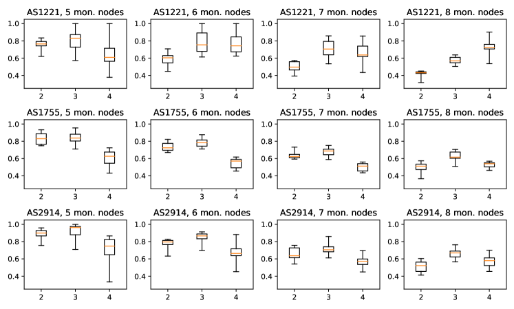
Figure 2: Distributions of F1 scores of the routing matrix estimate for the 120 case studies, based on a sample of size 100,000. Plots in each row are based on the same underlying network, and plots in the same column have the same number of monitor nodes. The three boxes in each plot correspond to values $i_{\rm max}=2,3,4$ used for inference.

VI Results and Evaluation

What follows is an abbreviated set of experimental results applying Sparse Möbius Inference to many synthetic datasets. The full description of our methodology and results are contained in Appendix A (in the supplementary file).

Synthetic Datasets

We created 120 synthetic datasets based on real ISP network topologies, provided by Rocketfuel [26]. We selected three networks within the Rocketfuel database with different sizes and densities (AS1221, AS1755, and AS2914). For each topology, we generated 40 synthetic datasets of path delays: 10 each for experiments with 5, 6, 7, and 8 monitor nodes. For each of these 40 case studies, the network links are assigned different gamma delay distributions, the $n_{\rm node}$ monitor nodes are selected at random, and the $n=\binom{n_{\rm node}}{2}$ monitor paths are chosen by computing the shortest path between each pair of monitor nodes. Then a large sample of the joint path delay distribution is recorded.

Sparsity of the Common and Exact Cumulants

The Sparse Mob̈ius Inference procedure is based on the postulate that the vectors of common and exact cumulants are both sparse. This assumption holds up extremely well in our case studies; with $n=28$ paths, for example, 99.99% to 99.999% of the entries of the common cumulant vector are zero.

Evaluating the Bounding Topology

The first stage of Sparse Möbius Inference uses low-order cumulants to estimate $\operatorname{supp}(\mathbf{f}_{i})$. Our results indicate that Algorithm 3 is very effective at finding a bounding topology with a tight support estimate. For almost all of the 120 case studies, third-order cumulants $(i_{f}=3)$ with a sample size $N=50,000$ or larger are sufficient to construct a bounding topology that predicts $\operatorname{supp}(\mathbf{f}_{i})$ with an F1 score of 1.0 (or extremely close to 1.0).

Evaluating the Estimated Routing Matrix

Next, we evaluate the performance of Sparse Möbius Inference end-to-end. We ran stages 2 and 3 to get an estimate of $\hat{\mathbf{R}}$ for each case study and various sample sizes, using as input to Stage 2 the bounding topologies computed with $i_{f}=4$ from the same sample. The hyperparameters of the lasso heuristic ($\lambda$ and the exponent $b$) are tuned separately for each underlying network and number of monitor paths. Figure 2 shows the F1 scores that we obtained for each of the 120 case studies. For all underlying networks, the performance tends to degrade with the number of monitor paths, and the best estimate is usually obtained using third-order $k$-statistics ($i_{\rm max}=3$).

Evaluating the Lasso Heuristic

We also evaluated the lasso heuristic in Stage 3 using ground-truth cumulants. For these experiments, we borrowed the bounding topologies computed from the $N=100,000$ sample with $i_{f}=4$, but instead of populating the $\hat{\mathbf{f}}_{o}$ vector in (15) with $k$-statistics computed from this sample, we used the true common cumulants. These values have no uncertainty, so we removed the quadratic penalty from $J(\mathbf{f}_{o},\mathbf{f}_{u})$, instead constraining $\mathbf{f}_{o}=\hat{\mathbf{f}}_{o}$. Again, the hyperparameters $\lambda$ and $b$ are tuned separately for each network and number of monitor paths. Figure 3 plots the distribution of the resulting F1 scores. For smaller (5 or 6 monitor) scenarios, the lasso heuristic is typically capable of 100% accurate routing matrix reconstruction. For larger scenarios, the heuristic requires up to third-order cumulants for completely accurate inference.

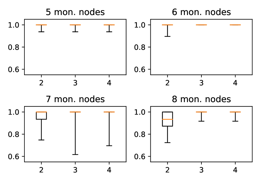
Figure 3: Distributions of F1 scores of the routing matrix estimate based on ground-truth cumulants (instead of $k$-statistics). Each plot corresponds to a particular number of monitor paths, and the results are aggregated across case studies from the 3 underlying networks. The three boxes in each plot correspond to values $i_{\rm max}=2,3,4$ used for inference.

Discussion

Our results paint a mixed but optimistic picture for the Sparse Möbius Inference procedure. Admittedly, higher F1 scores from the $N=100,000$ sample would be desirable before the method is deployed in real-world applications. But the two key components of the procedure—estimating $\operatorname{supp}(\mathbf{f}_{i})$ from low-order $k$-statistics, and using the lasso sparsity heuristic to infer $\mathbf{R}$ without using the high-order cumulants required by MIA—worked very well in isolation, achieving 100% accuracy in most scenarios.

VII Conclusion

We have provided a novel tomographic approach to routing topology inference from path delay data, without making any assumptions on routing behavior. Through MIA, we have provided a theoretical framework for extending the use of second-order statistics in network tomography toward higher-order statistics. Furthermore, we have introduced the Sparse Möbius Inference procedure, which implements a heuristic and more practical variant of MIA. We have extensively studied the performance of Sparse Möbius Inference using many synthetic case studies. While more work is needed to improve the filtering of noisy $k$-statistics, our results indicate that the Sparse Möbius Inference can serve as a solid foundation for future improvements.

References

- [1] X. Zhang and C. Phillips, “A survey on selective routing topology inference through active probing,” IEEE Communications Surveys & Tutorials, vol. 14, no. 4, pp. 1129–1141, 2011.
- [2] M. H. Gunes and K. Sarac, “Analyzing router responsiveness to active measurement probes,” in International Conference on Passive and Active Network Measurement, 2009, pp. 23–32.
- [3] M. Luckie, Y. Hyun, and B. Huffaker, “Traceroute probe method and forward ip path inference,” in ACM SIGCOMM Conference on Internet Measurement, 2008, pp. 311–324.
- [4] B. Yao, R. Viswanathan, F. Chang, and D. Waddington, “Topology inference in the presence of anonymous routers,” in IEEE Conf. on Computer Communications, 2003, pp. 353–363.
- [5] X. Jin, W.-P. K. Yiu, S.-H. G. Chan, and Y. Wang, “Network topology inference based on end-to-end measurements,” IEEE Journal on Selected Areas in Communications, vol. 24, no. 12, pp. 2182–2195, 2006.
- [6] B. Holbert, S. Tati, S. Silvestri, T. La Porta, and A. Swami, “Network topology inference with partial information,” IEEE Transactions on Network and Service Management, vol. 12, no. 3, pp. 406–419, 2015.
- [7] M. Coates, A. O. Hero III, R. Nowak, and B. Yu, “Internet tomography,” IEEE Signal Processing Magazine, vol. 19, no. 3, pp. 47–65, 2002.
- [8] S. Ratnasamy and S. McCanne, “Inference of multicast routing trees and bottleneck bandwidths using end-to-end measurements,” in IEEE Conf. on Computer Communications, 1999, pp. 353–360.
- [9] N. G. Duffield, J. Horowitz, F. Lo Presti, and D. Towsley, “Multicast topology inference from measured end-to-end loss,” IEEE Transactions on Information Theory, vol. 48, no. 1, pp. 26–45, 2002.
- [10] M. Coates, R. Castro, R. Nowak, M. Gadhiok, R. King, and Y. Tsang, “Maximum likelihood network topology identification from edge-based unicast measurements,” in ACM SIGMETRICS Performance Evaluation Review, 2002, pp. 11–20.
- [11] J. Ni, H. Xie, S. Tatikonda, and Y. R. Yang, “Efficient and dynamic routing topology inference from end-to-end measurements,” IEEE/ACM Transactions on Networking, vol. 18, no. 1, pp. 123–135, 2009.
- [12] M. G. Rabbat, M. J. Coates, and R. D. Nowak, “Multiple-source Internet tomography,” IEEE Journal on Selected Areas in Communications, vol. 24, no. 12, pp. 2221–2234, 2006.
- [13] G. Berkolaiko, N. Duffield, M. Ettehad, and K. Manousakis, “Graph reconstruction from path correlation data,” Inverse Problems, vol. 35, no. 1, p. 015001, 2018.
- [14] L. Ma, T. He, A. Swami, D. Towsley, and K. K. Leung, “Network capability in localizing node failures via end-to-end path measurements,” IEEE/ACM Transactions on Networking, vol. 25, no. 1, pp. 434–450, 2016.
- [15] A. Gkelias, L. Ma, K. K. Leung, A. Swami, and D. Towsley, “Robust and efficient monitor placement for network tomography in dynamic networks,” IEEE/ACM Transactions on Networking, vol. 25, no. 3, pp. 1732–1745, 2017.
- [16] A. Sabnis, R. K. Sitaraman, and D. Towsley, “OCCAM: An optimization based approach to network inference,” ACM SIGMETRICS Performance Evaluation Review, vol. 46, no. 2, pp. 36–38, 2019.
- [17] P. McCullagh and J. Kolassa, “Cumulants,” Scholarpedia, vol. 4, no. 3, p. 4699, 2009.
- [18] E. D. Nardo, G. Guarino, and D. Senato, “A new method for fast computing unbiased estimators of cumulants,” Statistics and Computing, vol. 19, no. 2, p. 155, 2009.
- [19] K. D. Smith, “A tutorial on multivariate -statistics and their computation,” 2020. [Online]. Available: http://arxiv.org/pdf/2005.08373
- [20] E. D. Nardo and G. Guarino, “kstatistics: Unbiased estimators for cumulant products,” 2019, R package version 1.0. [Online]. Available: https://CRAN.R-project.org/package=kStatistics
- [21] K. D. Smith, “PyMoments: A Python toolkit for unbiased estimation of multivariate statistical moments,” 2020. [Online]. Available: https://github.com/KevinDalySmith/PyMoments
- [22] B. Staude, S. Rotter, and S. Grün, “CuBIC: cumulant based inference of higher-order correlations in massively parallel spike trains,” Journal of Computational Neuroscience, vol. 29, no. 1-2, pp. 327–350, 2010.
- [23] M. H. DeGroot and M. J. Schervish, Probability and Statistics, 4th ed. Pearson Education, 2012.
- [24] A. C. Davison and D. V. Hinkley, Boostrap Methods and Their Application. Cambridge University Press, 1999.
- [25] Y. Zhang, D. Hatzinakos, and A. N. Venetsanopoulos, “Bootstrapping techniques in the estimation of higher-order cumulants from short data records,” in IEEE Int. Conf. on Acoustics, Speech and Signal Processing, vol. 4, 1993, pp. 200–203.
- [26] N. Spring, R. Mahajan, and D. Wetherall, “Measuring ISP topologies with Rocketfuel,” ACM SIGCOMM Computer Communication Review, vol. 32, no. 4, pp. 133–145, 2002.