Reachability as a Unifying Framework for Computing Helicopter Safe Operating Conditions and Autonomous Emergency Landing

Abstract

We present a numeric method to compute the safe operating flight conditions for a helicopter such that we can ensure a safe landing in the event of a partial or total engine failure. The unsafe operating region is the complement of the backwards reachable tube, which can be found as the sub-zero level set of the viscosity solution of a Hamilton–Jacobi (HJ) equation. Traditionally, numerical methods used to solve the HJ equation rely on a discrete grid of the solution space and exhibit exponential scaling with dimension, which is problematic for the high-fidelity dynamics models required for accurate helicopter modeling. We avoid the use of spatial grids by formulating a trajectory optimization problem, where the solution at each initial condition can be computed in a computationally efficient manner. The proposed method is shown to compute an autonomous landing trajectory from any operating condition, even in non-cruise flight conditions.

1 Introduction

This paper presents a method to efficiently compute unsafe operating flight conditions for which no control sequence exists to safely land the helicopter in the event of partial or total engine failure. A chart called a height-velocity diagram or H-V diagram needs to be produced for each airframe, and a human pilot can utilize the diagram to avoid operating in unsafe conditions. If operating in the safe region, there exists a control sequence to initiate an autorotation, whereby the helicopter enters a glide slope so as to maintain rotor inertia and then flare to slow down near the ground and land safely (FAA, 2019, Chapter 11). H-V diagrams are ultimately determined through flight testing, which is inherently dangerous since the test objective is to define the unsafe boundaries of flight operations. Therefore, there is a need to accurately compute the safe and unsafe regions directly from the helicopter dynamics, and construct a H-V diagram prior to flight testing. The capability to produce H-V diagrams is desired for aircraft that are in the early design stages and have not yet flown, aircraft that are already flying and preparing for an H-V flight test event, as well as refining the H-V diagram of operational aircraft. The capability is required for aircraft that do not have a representative, high-fidelity flight simulation, as well as for more mature aircraft for which a high-fidelity simulation is available.

We consider the safe region as any initial flight condition where there exists a control sequence that can steer the system to a safe landing condition, i.e. minimal vertical and horizontal velocity at the ground level, rotor near level, etc. Determining the set of states of a dynamical system that can be driven into a particular final condition is commonly referred to as reachability analysis, and reachable sets can be determined from the sub-zero level set of the viscosity solution to a Hamilton–Jacobi (HJ) partial differential equation (PDE) (Mitchell et al. (2005)).

Traditionally, these HJ PDEs are solved numerically by constructing a dense discrete grid of the solution space (Mitchell (2008)), and are supported by mature theory (Osher and Fedkiw (2006)). Despite this, HJ reachability analysis has suffered one critical draw-back: Computing the elements of a spatial grid scales poorly with dimension, and therefore have limited applicability for vehicle problems where the dimension of the state space is greater than four. The work of Harno and Kim (2018) attempted to compute helicopter safe operating regions using the grid-based method of Mitchell (2008), but was restricted to a two-dimensional state space, and therefore is not representative of actual helicopter motion and is not applicable for safety critical use.

Recent research based on generalizations of the Hopf formula (Hopf (1965)) have avoided a spatial grid of the state space and instead form a grid over time, where numerical solutions are obtained by constructing a trajectory optimization problem. These techniques were used in Darbon and Osher (2016) to compute solutions to the HJ equation for systems with state and time-independent Hamiltonians of the form $\dot{x}=f\left(u\left(t\right)\right)$, and Kirchner et al. (2018a) expanded the classes of systems to general linear systems in high-dimensions. Additionally, these methods were successfully applied to vehicle control problems such as collaborative pursuit-evasion (Kirchner et al. (2018b)) and coordination of heterogeneous groups of vehicles (Kirchner et al. (2020)).

The methods described above based on the Hopf formula can be seen as an optimization problem based on the costate trajectory of the system. We propose in this work to formulate an optimization of the state trajectory directly, which allows consideration of the non-linear dynamics encountered in helicopter motion. There is no need to directly formulate the optimal Hamiltonian of the system, since the Hamiltonian frequently resulting from helicopter dynamics does not have a standard form.

There have been various proposals to compute the H-V diagram using trajectory optimization (see e.g. Johnson (1977); Lee et al. (1988); Carlson et al. (2006); Yomchinda (2013); Bibik and Narkiewicz (2012)), but they suffer several drawbacks. These methods minimize cost functionals with weighted cost terms and a terminal state constraint, which do not guarantee necessary ground landing conditions are met. Therefore, the solution of these optimization problems do not, in general, give the reachable set. Since the functional is parameterized by the terminal state at precisely terminal time, $t$, time is an unknown free parameter that must be solved for. When combined with the terminal constraint, it is not guaranteed that a candidate trajectory is feasible for a particular time and numeric convergence issues can be observed.

We propose to construct an implicit surface representation of the desired safe landing condition and, in doing so, create a trajectory optimization that gives the backwards reachable tube (Bansal et al. (2017)). We consider the case where the time-to-land need not be known a priori by considering that the intersection of the helicopter with the ground could occur at any time on the interval $\left[0,\infty\right)$. We utilize Lagrange polynomials to create a collocation scheme that converges rapidly with the number of time samples and can represent the required half-infinite time intervals. From this we compute the optimal landing sequence to autonomously achieve a safe landing from any initial condition that is within the backwards reachable tube.

2 Reachability and Safe Operating Regions

We consider helicopter dynamics

$$\frac{d}{ds}x\left(s\right)=f\left(x\left(s\right),u\left(s\right)\right),$$ (1)

for $s\in\left[0,t\right]$ where $x\in\mathbb{R}^{n}$ is the system state and $u\left(s\right)\in\mathcal{U}\subset\mathbb{R}^{m}$ is the control input, constrained to lie in the admissible control set $\mathcal{U}$. We denote by $\gamma$ the state trajectory $\left[0,t\right]\ni s\mapsto$ $\gamma\left(s;x,u\left(\cdot\right)\right)\in\mathbb{R}^{n}$ that evolves in time with measurable control input $\left[0,s\right]\mapsto u\left(\cdot\right)\in\mathcal{U}$ according to $\left(\ref{eq:general dynamics}\right)$ starting from initial state $x$ at $s=0$. The trajectory $\gamma$ is a solution of $\left(\ref{eq:general dynamics}\right)$ in that it satisfies $\left(\ref{eq:general dynamics}\right)$ almost everywhere:

$$\frac{d}{ds}\gamma\left(s;x,u\left(\cdot\right)\right) =f\left(\gamma\left(s;x,u\left(\cdot\right)\right),u\left(s\right)\right),$$ (2)

$$\gamma\left(0;x,u\left(\cdot\right)\right) =x.$$

We denote by $\Theta_{0}\subseteq\mathbb{R}^{n}$ as the goal set that represents the set of acceptable safe landing conditions. We seek to determine if a control sequence exists that drives the system into $\Theta_{0}$ at exactly time $t$. The set of all initial states where there exists a control to drive the system to the set at exactly time $t$ is called the backward reachable set (BRS) of the system and is defined as

$$\Theta_{S}\left(t\right)=\left\{x:\exists u\left(\cdot\right)\in\mathcal{U},\gamma\left(t;x,u\left(\cdot\right)\right)\in\Theta_{0}\right\}.$$ (3)

2.1 The Connection of the BRS to the HJ Equation

We represent the set of safe landing conditions, $\Theta_{0}$, implicitly with the function $J:\mathbb{R}^{n}\rightarrow\mathbb{R}$ such that

$$\Theta_{0}=\left\{x\in\mathbb{R}^{n}|J\left(x\right)\leq 0\right\}$$ (4)

and use it to construct a cost functional for the system trajectory $\gamma\left(s;x,u\left(\cdot\right)\right)$, given terminal time $t$ as

$$K\left(t,x,u\left(\cdot\right)\right)=\int_{0}^{t}\mathcal{I}_{\mathcal{U}}\left(u\left(s\right)\right)ds+J\left(\gamma\left(t;x,u\left(\cdot\right)\right)\right),$$ (5)

where the running cost function $\mathcal{I}_{\mathcal{U}}:\mathbb{R}^{m}\rightarrow\mathbb{R}\cup\left\{+\infty\right\}$ is the characteristic function for the set $\mathcal{U}$ and is defined by

$$\mathcal{I}_{\mathcal{U}}\left(u\right)=\begin{cases}0&\text{if}\,u\in\mathcal{U}\\ +\infty&\text{otherwise.}\end{cases}$$

The value function $\varphi:\mathbb{R}^{n}\times\left[0,t\right]\rightarrow\mathbb{R}$ is defined as the minimum cost, $K$, among all admissible controls for a given state $x$ as

$$\varphi\left(x,t\right)=\underset{u\left(\cdot\right)\in\mathcal{U}}{\text{inf}}\,K\left(t,x,u\left(\cdot\right)\right).$$ (6)

The value function in $\left(\ref{eq: Value function}\right)$ satisfies the dynamic programming principle (Evans (2010)) and also satisfies the following initial value Hamilton–Jacobi (HJ) equation with $\varphi$ being the viscosity solution of

$$\begin{cases}\frac{\partial\varphi}{\partial s}\left(x,s\right)+H\left(x,\nabla_{x}\varphi\left(x,s\right)\right)=0,\\ \varphi\left(x,0\right)=J\left(x\right),\end{cases}$$ (7)

for $s\in\left[0,t\right]$, where the Hamiltonian $H:\mathbb{R}^{n}\times\mathbb{R}^{n}\rightarrow\mathbb{R}\cup\left\{+\infty\right\}$ is defined by

$$H\left(x,p\right)=\underset{u\in\mathcal{U}}{\text{sup}}\left\langle-f\left(x,u\right),p\right\rangle,$$ (8)

where we denote by $p\in\mathbb{R}^{n}$ the costate variable.

Fact 1 (Mitchell (2007a))

The zero sub level sets of the viscosity solution $\varphi\left(x,t\right)$ is an implicit surface representation of the finite time backwards reachable set, $\Theta_{S}\left(t\right)$ defined in $\left(\ref{eq: formal definition of BRS}\right)$.

We note here the important distinction that the BRS in $\left(\ref{eq: formal definition of BRS}\right)$ defines the set of initial states that can be driven into the set $\Theta_{0}$ at precisely time $t$. It is possible for the system to be driven into the set $\Theta_{0}$ at an earlier time $\tilde{t}<t$ and then later exit the set $\Theta_{0}$. This motivated the characterization of the backwards reachable tube in Mitchell et al. (2005).

2.2 The Backwards Reachable Tube

We are instead interested if the system can be driven into $\Theta_{0}$ at any time on the range $[0,t]$. This set of initial states, coined the backwards reachable tube (BRT) in Bansal et al. (2017), is defined by

$$\Theta_{T}\left(t\right)=\left\{x:\exists u\left(\cdot\right)\in\mathcal{U},\exists s\in\left[0,t\right],\gamma\left(s;x,u\left(\cdot\right)\right)\in\Theta_{0}\right\}.$$ (9)

The seminal work of Mitchell et al. (2005) showed that the backwards reachable tube is found from the zero sub level set of $\varphi\left(x,t\right)$, which is the viscosity solution to the following modified Hamilton–Jacobi equation

$$\begin{cases}\frac{\partial\varphi}{\partial s}\left(x,s\right)+\max\left(0,H\left(x,\nabla_{x}\varphi\left(x,s\right)\right)\right)=0,\\ \varphi\left(x,0\right)=J\left(x\right),\end{cases}$$ (10)

with $H\left(x,p\right)$ the same as given above in $\left(\ref{eq: Basic Hamiltonian definition}\right)$. The intuition is that the value function cannot decrease, which does not allow the level sets to contract. It can be seen that any trajectory that enters the set $\Theta_{0}$ is not allowed to escape by “freezing” it in time. The reachable set and reachable tube are connected through the following relation (Mitchell, 2007b, Proposition 1)

$$\Theta_{T}\left(t\right)=\bigcup_{s\in\left[0,t\right]}\Theta_{S}\left(s\right).$$ (11)

The boolean set operation in $\left(\ref{eq:Tube is union of sets}\right)$ implies a corresponding property (Osher and Fedkiw (2006)) of the implicit surface representations

$$\varphi_{T}\left(x,t\right)=\underset{s\in\left[0,t\right]}{\min}\varphi_{S}\left(x,s\right).$$ (12)

The backwards reachable tube, $\Theta_{T}\left(t\right)$, characterizes the controllably safe regions of flight. Therefore, the set of unsafe states is found from

$$\Theta^{C}:=\underset{t\rightarrow\infty}{\lim}\mathbb{R}^{n}\setminus\Theta_{T}\left(t\right).$$

3 Computing the Reachable Tube Through Optimization

Under a mild set of regularity conditions (Subbotin, 1995, Ch. 7, p. 63), $\varphi\left(x,s\right)$ is the unique viscosity solution of $\left(\ref{eq:Initial value HJ PDE}\right)$ (Subbotin, 1995, Th. 8.1, p. 70). The uniqueness of the solution, $\varphi\left(x,s\right)$, implies that the viscosity solution is equivalent to the value function and can be found by minimizing $\left(\ref{eq: Cost Function}\right)$ with constraints given by $\left(\ref{eq:dynamic constraints}\right)$. The HJ of the BRT in $\left(\ref{eq:mitchell HJ equation fro BRT}\right)$ can be constructed by augmenting the dynamics of $\left(\ref{eq:general dynamics}\right)$ with

$$\frac{d}{ds}x\left(s\right)=g\left(x\left(s\right),u\left(s\right),a\left(s\right)\right):=a\left(s\right)f\left(x\left(s\right),u\left(s\right)\right),$$ (13)

where $\left[0,t\right]\ni s\mapsto a\left(s\right)\in\left[0,1\right]$ is measurable scalar function (Mitchell et al. (2005)). We denote by $\zeta$ the state trajectory of the augmented system $\left(\ref{eq:augmented dynamics}\right)$ that satisfies

$$\frac{d}{ds}\zeta\left(s;x,u\left(\cdot\right),a\left(\cdot\right)\right) =g\left(\zeta\left(s;x,u\left(\cdot\right),a\left(\cdot\right)\right),u\left(s\right),a\left(s\right)\right),$$

$$\zeta\left(0;x,u\left(\cdot\right),a\left(\cdot\right)\right) =x.$$ (14)

Note that since $a$ is constrained to $\left[0,1\right]$, a value of $a=1$ makes the augmented dynamics of $\left(\ref{eq:augmented dynamics}\right)$ equivalent to the original dynamics of $\left(\ref{eq:general dynamics}\right)$ and if $a=0$ the dynamics stop completely. We denote by

$$\sigma\left(s\right):=\int_{0}^{s}a\left(\ell\right)d\ell,$$

the pseudotime variable, and denote by $\sigma^{\dagger}$ as a quasi-inverse of $\sigma$ in the sense that

$$\sigma^{\dagger}\left(\sigma\left(s\right)\right)=s.$$

The formal definition of this quasi-inverse is given in (Mitchell et al., 2005, Lemma 6), and it was shown that the trajectories of $\left(\ref{eq:augmented dynamic constraints}\right)$ have the following relations

$$\gamma\left(\sigma\left(s\right);x,u\left(\sigma^{\dagger}\left(\cdot\right)\right)\right)=\zeta\left(s;x,u\left(\cdot\right),a\left(\cdot\right)\right),$$

for any $s\in\left[0,t\right]$ (Mitchell et al., 2005, Lemma 4), and consequently $\zeta$ visits only a subset states of the $\gamma$ (Mitchell et al., 2005, Corollary 5). Therefore, we can solve the modified optimization problem to find the reachable tube:

$$\begin{cases}\underset{u\left(\cdot\right),a\left(\cdot\right)}{\min}&J\left(\zeta\left(t;x,u\left(\cdot\right),a\left(\cdot\right)\right)\right)\\ \text{Subject to}&\frac{d}{ds}\zeta\left(s\right)=g\left(\zeta\left(s\right),u\left(s\right),a\left(s\right)\right)\\ &\zeta\left(0\right)=x\\ &u\left(\cdot\right)\in\mathcal{U}\\ &a\left(\cdot\right)\in\left[0,1\right]\\ &\dot{a}\left(\cdot\right)\leq 0,\end{cases}$$ (15)

where the last line of $\left(\ref{eq:modified optimization}\right)$ is an optional regularization term since the optimal $a\left(\cdot\right)$ is not unique.

3.1 Time-Domain Transformation

We use collocation to approximate the trajectory $\zeta$ and first perform a time domain transformation which maps $s\in\left[0,\infty\right)$ into the computation interval $\tau\in\left[-1,1\right)$ with the invertible transform defined as

$$s=\Gamma^{-1}\left(\tau\right)=c\log\left(\frac{2}{1-\tau}\right),$$ (16)

where the choice of $\Gamma$ is a scaled version of that proposed in Garg et al. (2011). The dynamics $\left(\ref{eq:augmented dynamics}\right)$ are similarly transformed with

$$\frac{d}{d\tau}x\left(\tau\right) =\frac{d}{d\tau}\Gamma\left(\tau\right)g\left(x\left(\tau\right),u\left(\tau\right),a\left(\tau\right)\right),$$

and with the transform defined in $\left(\ref{eq:time domain transformation}\right)$ becomes

$$\frac{d}{d\tau}x\left(\tau\right)=\frac{c}{\left(1-\tau\right)}g\left(x\left(\tau\right),u\left(\tau\right),a\left(\tau\right)\right).$$

Hereafter, we assume that the trajectory, $\zeta$, is a solution to the transformed dynamics satisfying

$$\frac{d}{d\tau}\zeta\left(\tau;x,u\left(\cdot\right),a\left(\cdot\right)\right) =\frac{c}{\left(1-\tau\right)}$$

$$\times g\left(\zeta\left(\tau;x,u\left(\cdot\right),a\left(\cdot\right)\right),u\left(\tau\right),a\left(\tau\right)\right)$$

$$\zeta\left(-1;x,u\left(\cdot\right),a\left(\cdot\right)\right) =x.$$

3.2 Finite Trajectory Approximation

We propose a polynomial trajectory approximation, which is commonly referred to as pseudospectral optimal control, and was introduced in Elnagar et al. (1995) and later refined in Ross and Karpenko (2012) and Garg et al. (2010). We denote by $\zeta^{N}$ as the approximation to $\zeta$ with Lagrange polynomials as

$$\zeta\left(\tau\right)\approx\zeta^{N}\left(\tau\right)=\sum_{j=0}^{N}x_{j}L_{j}\left(\tau\right),$$ (17)

defined by a set of $N$ points, $x_{j}=\zeta\left(\tau_{j};x,u\left(\cdot\right),a\left(\cdot\right)\right)$, sampled on the time grid

$$\pi^{N}=\left\{\tau_{j}:j=0,\ldots,N\right\},$$

where each $\tau_{j}\in\left[-1,1\right]$. The Lagrange basis functions are given as

$$L_{j}\left(\tau\right):=\prod_{\underset{k\neq j}{k=0}}^{N}\frac{\tau-\tau_{k}}{\tau_{j}-\tau_{k}},$$

and it follows that

$$\frac{d}{d\tau}\zeta^{N}\left(\tau_{i}\right)=\sum_{j=0}^{N}x_{j}\dot{L}_{j}\left(\tau_{i}\right)=\sum_{j=0}^{N}D_{ij}x_{j},$$

where we denote by $D\in\mathbb{R}^{N\times\left(N+1\right)}$ as the Gauss differentiation matrix constructed with each element, with row $i$ and column $j$, given by

$$D_{ij}:=\dot{L}_{j}\left(\tau_{i}\right).$$ (18)

We select $\pi^{N}$ as Legendre-Gauss-Radau (LGR) points with $\pi^{N}$ and the corresponding differentiation matrix, $D$, and quadrature weights, $w$, are found from (Shen et al., 2011, Section 3.3). Note that since LGR points do not include a point at $\tau=1$, we avoid a singularity in $\left(\ref{eq:time domain transformation}\right)$ at $t\rightarrow\infty$. We denote by $D_{0}\in\mathbb{R}^{N\times 1}$ as the first column of $D$ corresponding to the boundary condition and denote by $D_{I}\in\mathbb{R}^{N\times N}$ as the remaining columns representing the interior nodes such that

$$D=\left[\begin{array}[]{cc}D_{0}&D_{I}\end{array}\right].$$ (19)

We denote by $X\in\mathbb{R}^{n\cdot N}$ as the concatenated vector of all collocation points for $j=1,\ldots,N$ given as

$$X:=\left(x_{1},\cdots,x_{N}\right)^{\top},$$ (20)

and likewise denote $U\in\mathbb{R}^{m\cdot\left(N+1\right)}$ as the concatenated vector of all the collocated control input points

$$U:=\left(u_{0},\cdots,u_{N}\right)^{\top},$$

where each $u_{j}$ is the control input at each time $\tau_{j}\in\pi^{N}$. And similarly, for the augmented inputs, $a_{j}$, we have

$$A:=\left(a_{0},\cdots,a_{N}\right)^{\top}.$$

Recall that $x_{0}=x=\zeta\left(-1;x,u\left(\cdot\right),a\left(\cdot\right)\right)$. We denote by $G\left(X,U,A\right)$ as the concatenated vector of the equations of motion,

$$G\left(X,U,A\right):=\left[\begin{array}[]{c}a_{0}\frac{c}{\left(1-\tau_{0}\right)}f\left(x,u_{0}\right)\\ a_{1}\frac{c}{\left(1-\tau_{1}\right)}f\left(x_{1},u_{1}\right)\\ \vdots\\ a_{N}\frac{c}{\left(1-\tau_{N}\right)}f\left(x_{N},u_{N}\right)\end{array}\right],$$

evaluated at each point in $\tau_{j}\in\pi^{N}$. It follows the differentiation matrix $\left(\ref{eq:diff matrix partition}\right)$ of the concatenated of state $\left(\ref{eq: concat state}\right)$ is

$$\mathcal{D}_{I}=D_{I}\otimes I_{n},$$

where $\otimes$ denotes the Kronecker product and $I_{n}$ is the $n\times n$ identity matrix. Likewise, we have

$$\mathcal{D}_{0}=D_{0}\otimes I_{n}.$$

The dynamic equality constraint is now written as

$$\mathcal{D}_{s}X+\mathcal{D}_{0}x=G\left(X,U,A\right).$$

Recall that $w$ is the vector of LGR quadrature weights. It was proposed in Garg et al. (2010) to estimate the terminal state with

$$x_{N+1}=x+\left(w^{\top}\otimes I_{n}\right)G\left(X,U,A\right).$$

With $x=\zeta\left(0;x,u\left(\cdot\right),a\left(\cdot\right)\right)$ as the given initial condition, we construct the non-linear programming problem (NLP):

$$\begin{cases}\underset{X,U,A}{\min}&J\left(x_{N+1}\right)\\ \text{Subject to}&\mathcal{D}_{s}X+\mathcal{D}_{0}x=G\left(X,U,A\right)\\ &x_{N+1}=x+\left(w^{\top}\otimes I_{n}\right)G\left(X,U,A\right)\\ &u_{j}\in\mathcal{U}\\ &a_{j}\in\left[0,1\right]\\ &a_{j}-a_{j-1}\leq 0,\end{cases}$$ (21)

which has a numerical solution that approximates $\left(\ref{eq:modified optimization}\right)$ when $N$ is sufficiently large. The time of minimum cost in $\left(\ref{eq:implicit surface rep. of union property}\right)$ can be found from the following quadrature:

$$t^{*}=w^{\top}\left[\begin{array}[]{c}a_{0}\frac{c}{\left(1-\tau_{0}\right)}\\ \vdots\\ a_{N}\frac{c}{\left(1-\tau_{N}\right)}\end{array}\right].$$ (22)

4 Helicopter Dynamics

We define the state vector as $x=\left(y,v,\Omega,h,z,P\right)^{\top}\in\mathbb{R}^{6}$ with the vertical velocity, $y$; horizontal velocity, $v$; rotor angular speed, $\Omega$; height above ground level, $h$; horizontal displacement, $z$; and engine power, $P$. The control inputs are given as $u$=$\left(C_{T},\theta\right)^{\top}\in\mathbb{R}\times\left[0,2\pi\right)$ with thrust coefficient, $C_{T}$, effectively the collective control, and $\theta$, the aircraft pitch angle. Following Lee (1985), the dynamics are as follows:

$$f:\begin{cases}\dot{y}=g-\frac{\rho}{m}\left(\pi R^{2}\right)\left(\Omega R\right)^{2}C_{T}\cos\theta+\frac{1}{2}\frac{\rho}{m}f_{eh}V_{f}y\\ \dot{v}=\frac{\rho}{m}\left(\pi R^{2}\right)\left(\Omega R\right)^{2}C_{T}\sin\theta-\frac{1}{2}\frac{\rho}{m}f_{ez}V_{f}v\\ \dot{\Omega}=\frac{1}{I_{R}\Omega}\left(P-\frac{1}{\eta}\rho\left(\pi R^{2}\right)\left(\Omega R\right)^{3}C_{p}\right)\\ \dot{h}=-y\\ \dot{z}=v\\ \dot{P}=-\frac{1}{\kappa}P\end{cases}$$ (23)

where $\kappa$ denotes the engine response time constant, $\eta$ the rotor power efficiency factor, $m$ the mass of the helicopter, $V_{f}$ the velocity magnitude of the fuselage, $\sigma_{R}$ the rotor solidity, $R$ the rotor radius, $I_{R}$ the rotor inertia, $\rho$ the density of the air, and $g$ the acceleration due to gravity. $f_{eh}$ and $f_{ez}$ is the flat plat drag area in the vertical and horizontal directions, respectively. $C_{p}$ denotes the power coefficient defined as

$$C_{p}=\frac{1}{8}\sigma_{R}c_{d}+C_{T}\lambda,$$

where $c_{d}$ is the drag coefficient of the rotor airfoil and

$$\lambda=\frac{v\sin\theta-y\cos\theta+\nu}{\Omega R}$$

is the inflow ratio. The advance velocity, $U_{T}$, is given by

$$U_{T}=v\cos\theta+y\sin\theta.$$

The variable $\nu$ is induced velocity and we use the inflow model

$$\nu=\Omega R\sqrt{\frac{1}{2}C_{T}},$$

which is the ideal inflow in hover. More sophisticated inflow models exist but are outside the scope of this work, and the reader is encouraged to read Johnson (1977) and Chen and Hindson (1986) for more details.

5 Results

We ensure safe landing when the conditions $\left|y\right|\leq y_{\max}$ and $\left|v\right|\leq v_{\max}$ are met as the helicopter is sufficiently close to the ground; in this case $\left|h\right|\leq 1$. The parameters $y_{\max}$ and $v_{\max}$ are found from the structural specifications of the airframe. We select the function $J$ that satisfies $\left(\ref{eq:implicit surface def}\right)$ the terminal conditions with

$$J\left(x\right)=\max\left(\left|y\right|-y_{\max},\left|v\right|-v_{\max},\left|h\right|-1\right),$$

where, for this example, we chose $y_{\max}=8\,ft/s$ and $v_{\max}=6\,knots$. The remaining initial states are chosen as the trim conditions such that $\dot{y},\dot{v}=0$, and initial engine power was set $P_{0}=0$, simulating an instant engine failure and providing a safety factor as it gives the largest unsafe set. The input $C_{T}$ is bounded by a blade stall condition with $C_{T}\leq 0.15\sigma_{R}$ (Lee et al. (1988)), where $\left|\theta\right|\leq 40\textdegree$. The rest of the coefficients for the model in $\left(\ref{eq: heli eom}\right)$ are from (Yomchinda, 2013, Table 2-1, Table A-1). The number of interior time samples, $N$, is fixed at $24$ and the constant in $\left(\ref{eq:time domain transformation}\right)$ is set to $c=3$. To take advantage of the inherent sparsity of the formulated optimization, we use the NLP code IPOPT (Wächter and Biegler (2006)), where the constraint Jacobian was computed using automatic differentiation by the methods of Andersson et al. (2019).

The value function for the system was computed using the method of Section 3, and an H-V diagram is produced by finding the unsafe regions, which is all areas where the value function is greater than zero. Figure 1 shows the H-V diagram for the dynamics given in $\left(\ref{eq: heli eom}\right)$, where dark regions on the diagram represent initial height above ground level (AGL) and forward speed such that a safe landing in the event of an engine failure is impossible. Note that a disjoint lobe of the unsafe set appears on the bottom right of Figure 1 and is known as the high-speed unsafe region.

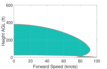
Figure 1: Shown in green is the set of unsafe H-V flight conditions as computed from the method of Section 3.

5.1 Autonomous Autorotation

The arguments that minimize $\left(\ref{eq:reach tube nlp}\right)$, denoted as $X^{*}$ and $U^{*}$, are the optimal landing trajectory and control sequence, respectively, provided that the helicopter is operating in the reachable tube. As an example we consider a helicopter in a trimmed cruise at $h=500\,ft$ with a forward speed of $75\,knots$. Figure 2 shows the state evolution as computed at the time of engine failure. The computed trajectory results in a safe landing in $9.06\,sec$ as found from $\left(\ref{eq:opt time}\right)$. We note the trajectory of the rotor speed, $\Omega$, in Figure 2c, where an increase in rotor speed is observed due to translational kinetic energy being transfered into rotational kinetic energy to successfully decelerate, or “flare”, at the terminal phase of the landing procedure.

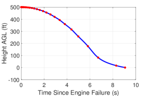
(a) Height profile during landing.

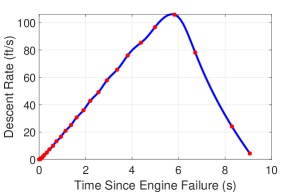
(b) Descent rate profile during landing.

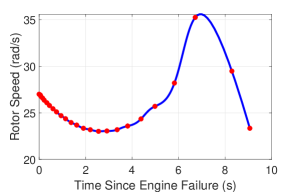
(c) Rotational speed of the helicopter rotor blades during landing.

Figure 2: Selected state trajectories of an autorotation after engine failure. Red dots indicate the points of $X$ as found by the NLP optimization. The blue line represents the Lagrange polynomial approximation, $\zeta^{N}$, of the time-transformed state trajectory.

6 Conclusion and Future Work

Presented is a numeric method for computing the backwards reachable tube for general non-linear systems. We are motivated by locating the unsafe operating states of a helicopter so they can be avoided by the pilot. By remaining outside of the unsafe set, it ensures it is possible to initiate an autorotation sequence after engine failure and guide the helicopter to a safe landing. The method can additionally be used to compute control inputs in order to complete an autonomous landing via autorotation. Future work includes augmenting $\left(\ref{eq: heli eom}\right)$ with human pilot dynamics as in McRuer and Krendel (1974) and include pilot reaction delay (Kirchner (2019)). Additionally, we will investigate integrating failure detection to initiate the autonomous autorotation landing procedure.

References

- FAA (2019) (2019). Rotorcraft Flying Handbook, FAA Manual H-8083-21B. Federal Aviation Administration.
- Andersson et al. (2019) Andersson, J.A.E., Gillis, J., Horn, G., Rawlings, J.B., and Diehl, M. (2019). CasADi – A software framework for nonlinear optimization and optimal control. Mathematical Programming Computation, 11(1), 1–36. 10.1007/s12532-018-0139-4.
- Bansal et al. (2017) Bansal, S., Chen, M., Herbert, S., and Tomlin, C.J. (2017). Hamilton-Jacobi reachability: A brief overview and recent advances. In IEEE 56th Annual Conference on Decision and Control (CDC), 2242–2253. IEEE.
- Bibik and Narkiewicz (2012) Bibik, P. and Narkiewicz, J. (2012). Helicopter optimal control after power failure using comprehensive dynamic model. Journal of Guidance, Control, and Dynamics, 35(4), 1354–1362.
- Carlson et al. (2006) Carlson, E.B., Xue, S., Keane, J., and Kevin, B. (2006). H-1 upgrades height-velocity diagram development through flight test and trajectory optimization. In Annual Forum Proceedings-American Helicopter Society, volume 62, 729. American Helicopter Society.
- Chen and Hindson (1986) Chen, R.T. and Hindson, W.S. (1986). Influence of dynamic inflow on the helicopter vertical response. Technical Report 88327, National Aeronautics and Space Administration.
- Darbon and Osher (2016) Darbon, J. and Osher, S. (2016). Algorithms for overcoming the curse of dimensionality for certain Hamilton-Jacobi equations arising in control theory and elsewhere. Research in the Mathematical Sciences, 3(1), 19.
- Elnagar et al. (1995) Elnagar, G., Kazemi, M.A., and Razzaghi, M. (1995). The pseudospectral Legendre method for discretizing optimal control problems. IEEE Transactions on Automatic Control, 40(10), 1793–1796.
- Evans (2010) Evans, L.C. (2010). Partial Differential Equations. American Mathematical Society, Providence, R.I.
- Garg et al. (2011) Garg, D., Hager, W.W., and Rao, A.V. (2011). Pseudospectral methods for solving infinite-horizon optimal control problems. Automatica, 47(4), 829–837.
- Garg et al. (2010) Garg, D., Patterson, M., Hager, W.W., Rao, A.V., Benson, D.A., and Huntington, G.T. (2010). A unified framework for the numerical solution of optimal control problems using pseudospectral methods. Automatica, 46(11), 1843–1851.
- Harno and Kim (2018) Harno, H.G. and Kim, Y. (2018). Safe flight envelope estimation for rotorcraft: A reachability approach. In 18th International Conference on Control, Automation and Systems (ICCAS), 998–1002. IEEE.
- Hopf (1965) Hopf, E. (1965). Generalized solutions of non-linear equations of first order. Journal of Mathematics and Mechanics, 14, 951–973.
- Johnson (1977) Johnson, W. (1977). Helicopter optimal descent and landing after power loss. Technical Report NASA-TM-X-73244, National Aeronautics and Space Administration.
- Kirchner (2019) Kirchner, M.R. (2019). A level set approach to online sensing and trajectory optimization with time delays. In IFAC-PapersOnline, volume 52, 301–306.
- Kirchner et al. (2020) Kirchner, M.R., Debord, M., and Hespanha, J.P. (2020). A Hamilton-Jacobi formulation for optimal coordination of heterogeneous multiple vehicle systems. arXiv preprint arXiv:2003.05792.
- Kirchner et al. (2018a) Kirchner, M.R., Hewer, G., Darbon, J., and Osher, S. (2018a). A primal-dual method for optimal control and trajectory generation in high-dimensional systems. In 2018 IEEE Conference on Control Technology and Applications (CCTA), 1583–1590. IEEE.
- Kirchner et al. (2018b) Kirchner, M.R., Mar, R., Hewer, G., Darbon, J., Osher, S., and Chow, Y.T. (2018b). Time-optimal collaborative guidance using the generalized Hopf formula. IEEE Control Systems Letters, 2(2), 201–206.
- Lee (1985) Lee, A.Y.N. (1985). Optimal Landing of a Helicopter in Autorotation. Ph.D. thesis, Department of Aeronautics and Astronautics. Stanford University.
- Lee et al. (1988) Lee, A.Y., Bryson, A.E., and Hindson, W.S. (1988). Optimal landing of a helicopter in autorotation. Journal of Guidance, Control, and Dynamics, 11(1), 7–12.
- McRuer and Krendel (1974) McRuer, D.T. and Krendel, E.S. (1974). Mathematical models of human pilot behavior. AGARDDograph 188, Advisory Group on Aerospace Research and Development.
- Mitchell et al. (2005) Mitchell, I., Bayen, A.M., and Tomlin, C.J. (2005). A time-dependent Hamilton-Jacobi formulation of reachable sets for continuous dynamic games. IEEE Transactions on Automatic Control, 50(7), 947–957.
- Mitchell (2007a) Mitchell, I.M. (2007a). A toolbox of level set methods. Technical Report TR-2007-11, UBC Department of Computer Science.
- Mitchell (2008) Mitchell, I.M. (2008). The flexible, extensible and efficient toolbox of level set methods. Journal of Scientific Computing, 35(2), 300–329.
- Mitchell (2007b) Mitchell, I.M. (2007b). Comparing forward and backward reachability as tools for safety analysis. In International Workshop on Hybrid Systems: Computation and Control, 428–443. Springer.
- Osher and Fedkiw (2006) Osher, S. and Fedkiw, R. (2006). Level Set Methods and Dynamic Implicit Surfaces, volume 153. Springer Science & Business Media.
- Ross and Karpenko (2012) Ross, I.M. and Karpenko, M. (2012). A review of pseudospectral optimal control: From theory to flight. Annual Reviews in Control, 36(2), 182–197.
- Shen et al. (2011) Shen, J., Tang, T., and Wang, L.L. (2011). Spectral Methods: Algorithms, Analysis and Applications, volume 41. Springer Science & Business Media.
- Subbotin (1995) Subbotin, A.I. (1995). Generalized Solutions of First Order PDEs: The Dynamical Optimization Perspective. Birkhäuser.
- Wächter and Biegler (2006) Wächter, A. and Biegler, L.T. (2006). On the implementation of an interior-point filter line-search algorithm for large-scale nonlinear programming. Mathematical Programming, 106(1), 25–57.
- Yomchinda (2013) Yomchinda, T. (2013). Real-time Path Planning and Autonomous Control for Helicopter Autorotation. Ph.D. thesis, Department of Aerospace Engineering, Pennsylvania State University.