Generalizing The Davenport-Mahler-Mignotte Bound – The Weighted Case

Abstract.

Root separation bounds play an important role as a complexity measure in understanding the behaviour of various algorithms in computational algebra, e.g., root isolation algorithms. A classic result in the univariate setting is the Davenport-Mahler-Mignotte (DMM) bound. One way to state the bound is to consider a directed acyclic graph $(V,E)$ on a subset of roots of a degree $d$ polynomial $f(z)\in{\mathbb{C}}[z]$, where the edges point from a root of smaller absolute value to one of larger absolute, and the in-degrees of all vertices is at most one. Then the DMM bound is an amortized lower bound on the following product: $\prod_{(\alpha,\beta)\in E}|\alpha-\beta|$. However, the lower bound involves the discriminant of the polynomial $f$, and becomes trivial if the polynomial is not square-free. This was resolved by Eigenwillig, (2008), by using a suitable subdiscriminant instead of the discriminant. Escorcielo-Perrucci, 2016, further dropped the in-degree constraint on the graph by using the theory of finite differences. Emiris et al., 2019, have generalized their result to handle the case where the exponent of the term $|\alpha-\beta|$ in the product is at most the multiplicity of either of the roots. In this paper, we generalize these results by allowing arbitrary positive integer weights on the edges of the graph, i.e., for a weight function $w:E\rightarrow{\mathbb{Z}}_{>0}$, we derive an amortized lower bound on $\prod_{(\alpha,\beta)\in E}|\alpha-\beta|^{w(\alpha,\beta)}$. Such a product occurs in the complexity estimates of some recent algorithms for root clustering (e.g., Becker et al., 2016), where the weights are usually some function of the multiplicity of the roots. Because of its amortized nature, our bound is arguably better than the bounds obtained by manipulating existing results to accommodate the weights.

1. Introduction

Given a monic univariate polynomial $f(z)\in{\mathbb{C}}[z]$, of degree $d$ with roots $\alpha_{1},\ldots,\alpha_{d}$, not all distinct, a root separation bound is a lower bound on the smallest distance $\text{sep}(f)$ between any distinct pair of roots of $f$. A classic result (Mignotte, 1992) states that

$$\text{sep}(f)>d^{-(d+2)/2}\Delta(f)^{1/2}M(f)^{1-d},$$

where

$$\Delta(f){\color[rgb]{1,0,0}\mathop{\mbox{\rm:=}}}\prod_{i<j}(\alpha_{i}-\alpha_{j})^{2}$$

is the discriminant of $f$, and

(1) $$M(f){\color[rgb]{1,0,0}\mathop{\mbox{\rm:=}}}\prod_{i=1}^{d}\max\left\{1,|\alpha_{i}|\right\}$$

is the Mahler measure of $f$.

The parameter $\text{sep}(f)$ naturally occurs in the complexity analysis of many algorithms; examples are the (real or complex) root isolation algorithms ((Pan, 2002), (Davenport, 1985), (Eigenwillig et al., 2006), (Becker et al., 2018)). However, most of these algorithms need a lower bound on the product of certain pairs of roots and not just the worst case separation. To capture these pairs, we consider a simple (i.e., no loops and multiple edges) undirected graph $G=(V,E)$, whose vertices are a subset of the distinct roots of $f$. Then we want a lower bound on $\prod_{(\alpha_{i},\alpha_{j})\in E}|\alpha_{i}-\alpha_{j}|$. One straightforward lower bound is $\text{sep}(f)^{|E|}$, but Davenport (Davenport, 1985) used the amortized nature of the Mahler measure to derive a lower bound for real roots that essentially matches the lower bound on $\text{sep}(f)$ given above; the argument was later modified by Mignotte to complex roots (Mignotte, 1995). A consequence of these results is a straightforward improvement in the complexity bounds on the running time of algorithms for root isolation algorithms by a multiplicative factor of the degree.

Both these lower bounds, nevertheless, rely on the discriminant $\Delta(f)$ and are trivial when the polynomial is not square-free, i.e., it has multiple roots. A remedy is to work with the square-free part ${\widehat{f}}$ of $f$, but this again blows the bound by exponential factors because of the growth in the coefficients of ${\widehat{f}}$ as compared to $f$. An alternative was presented by Eigenwillig (Eigenwillig, 2008) that uses the $(d-r)$-th sub-discriminant of $f$ instead of the the discriminant, where $r$ is the number of distinct roots of $f$. However, there are some constraints on the graph $G$ for the bound to be applicable, namely, in the directed acyclic graph obtained by directing the edges of $G$ from a root of smaller absolute value to one of larger absolute value, the in-degree of all the vertices is at most one. Escorcielo-Perrucci (Escorcielo and Perrucci, 2017) dropped this in-degree constraint by using the theory of finite differences. Despite this, their result gives weaker bounds on products of the form

(2) $$\prod_{(\alpha_{i},\alpha_{j})\in E}|\alpha_{i}-\alpha_{j}|^{w(\alpha_{i},\alpha_{j})},$$

where $w:E\rightarrow{\mathbb{N}}$ is a weight function that assigns a positive integer to all the edges. In the special case where the weight function is such that the weight of an edge is bounded by the multiplicity of one of its vertices, (Kobel and Sagraloff, 2015) and (Emiris et al., 2019) have derived lower bounds when the coefficients of $f$ are real and complex numbers, respectively. To state their bound, let $f$ have $r$ distinct roots $\alpha_{1},\ldots,\alpha_{r}$ with multiplicities $m_{1},\ldots,m_{r}$, respectively, ${\widehat{f}}$ denote the square-free part of $f$, and for a root $\alpha_{i}$ let $\Delta_{i}$ denote the distance to the nearest distinct root. Then the bound in (Emiris et al., 2019) is the following: If $K\subseteq[r]$ and $w_{i}\in{\mathbb{N}}$ is such that $w_{i}\leq m_{i}$, for $i\in K$, then

(3) $$\prod_{i\in K}\Delta_{i}^{w_{i}}\geq 2^{-d(r+2)}(\|f\|_{\infty}\|{\widehat{f}}\|_{\infty})^{-d}M(f)^{1-r}|\text{res}(f,{\widehat{f}}^{\prime})|,$$

here $\|\cdot\|_{\infty}$ is the maximum absolute value over the coefficient sequence of the polynomial, and $\text{res}(\cdot,\cdot)$ is the univariate resultant. These bounds, though useful, fail to provide amortized lower bounds when the $w_{i}$’s exceed the multiplicity. Such a scenario, for instance, occurs in the complexity analysis of some recent root clustering algorithms (Becker et al., 2018; Batra and Sharma, 2019), where the following product occurs, for some subsets $K_{i}\subseteq[r]$:

$$\prod_{i\in K}\Delta_{i}^{\sum_{j\in K_{i}}m_{j}}.$$

One way to derive a lower bound on this product is to exponentiate the left-hand side of (3) to the degree $d$ (since the sum of the multiplicities over $K_{i}$ is bounded by $d$), move the extraneous factors to the denominator in the right-hand side, and upper bound these to get a lower bound on the desired product. But, just as was the case with $\text{sep}(f)^{|E|}$ earlier, such an approach loses the amortization property and gives exponentially worse bounds.

In this paper, we derive a lower bound on the product in (2) for arbitrary weight functions. The restrictions on the weights in the earlier approaches was an outcome of the choice of the symmetric function (either the discriminant, sub-discriminant or the resultant). We instead choose a symmetric function based on the weights and try to optimize over all valid choices of the function. This is done by constructing a confluent Vandermonde matrix to get the desired weight structure in the exponents. The choice of the confluent Vandermonde is especially helpful when the weights are skewed in distribution, because this means we can pick a different multiplicity structure on the roots and obtain better bounds. The spectral structure of the weighted adjacency matrix $A_{w}{\color[rgb]{1,0,0}\mathop{\mbox{\rm:=}}}[w_{i,j}]_{i,j=1,\ldots,r}$ plays an important role in the choice of the multiplicity structure for constructing the confluent Vandermonde matrix. For ease of comprehension, we state our result when $f$ is an integer polynomial (since then the absolute value of the non-zero symmetric function is at least one, which is how the bounds are used in practice) and is also monic (otherwise divide $M(f)$ by the absolute value of the leading coefficient). Let $\|A_{w}\|_{\star}$ denote the nuclear norm of $A_{w}$, i.e., the sum of its singular values, $n{\color[rgb]{1,0,0}\mathop{\mbox{\rm:=}}}r\left\lceil{\sqrt{\|A_{w}\|_{\star}}}\right\rceil$, and $w(E)$ be the sum of the weights over the edges of $G$. Then we show that

(4) $$\prod_{(\alpha_{i},\alpha_{j})\in E}|\alpha_{i}-\alpha_{j}|^{w(\alpha_{i},\alpha_{j})}>M(f)^{-2r\|A_{w}\|_{\star}}\left({\frac{n}{\sqrt{3}}}\right)^{-\frac{3r\|A_{w}\|_{\star}}{2}-w(E)}n^{-n/2}.$$

The bound is amortized because the exponent of the Mahler measure does not contain $w(E)$, which would be the case if we try to derive the lower bound by modifying the earlier results (see (11) below).

In the next section, we give the requisite details and properties of the confluent Vandermonde matrix; Section 3 contains the statement of our main result Theorem 3.2 and its comparison with a modification of an existing bound; Section 4 contains a proof of the main result, and in Section 4.1 we specialize it to obtain the form given above in (4).

2. Confluent Vandermonde

Consider the column vector

$$v(x)^{t}{\color[rgb]{1,0,0}\mathop{\mbox{\rm:=}}}\left[\begin{array}[]{ccccccccccccccccccccccccc}1&x&x^{2}&\cdots&x^{n}\\ \end{array}\right].$$

Define the vector obtained by differentiating each entry in the column above $i$ times and dividing by $i!$, ie.,

(5) $$v_{i}(x)^{t}{\color[rgb]{1,0,0}\mathop{\mbox{\rm:=}}}\left[\begin{array}[]{ccccccccccccccccccccccccc}{0\choose i}x^{-i}&{1\choose i}x^{1-i}&{2\choose i}x^{2-i}&\cdots&{n-1\choose i}x^{n-1-i}\\ \end{array}\right],$$

with the natural convention that ${j\choose i}=0$ if $j<i$. Let

$${\boldsymbol{\beta}}{\color[rgb]{1,0,0}\mathop{\mbox{\rm:=}}}(\beta_{1},\ldots,\beta_{r})\in{\mathbb{C}}^{r}$$

be an $r$-dimensional vector of complex numbers,

$${\boldsymbol{\mu}}{\color[rgb]{1,0,0}\mathop{\mbox{\rm:=}}}(\mu_{1},\ldots,\mu_{r})\in{\mathbb{N}}^{r}$$

be a sequence of positive integers, and $n{\color[rgb]{1,0,0}\mathop{\mbox{\rm:=}}}\sum_{i}\mu_{i}$. Then the confluent Vandermonde matrix $V({\boldsymbol{\beta}};{\boldsymbol{\mu}})$ is the $n\times n$ matrix with columns $(v_{j}(\beta_{i}))$, where $1\leq i\leq r$ and $0\leq j\leq\mu_{i}-1$. We will also use the notation $V(\beta_{1},\ldots,\beta_{r};\mu_{1},\ldots,\mu_{r})$ when we want to emphasize the $\beta_{i}$’s and $\mu_{i}$’s. We illustrate it below for $r=3$ and $\mu_{1}=2,\mu_{2}=3$.

$$V({\boldsymbol{\beta}},{\boldsymbol{r}})=\left[\begin{array}[]{ccccccccccccccccccccccccc}1&0&1&0&0\\ \beta_{1}&1&\beta_{2}&1&0\\ \beta_{1}^{2}&{2\choose 1}\beta_{1}&\beta_{2}^{2}&2\beta_{2}&1\\ \beta_{1}^{3}&{3\choose 1}\beta_{1}^{2}&\beta_{2}^{3}&3\beta_{2}^{2}&{3\choose 2}\beta_{2}\\ \beta_{1}^{4}&{4\choose 1}\beta_{1}^{3}&\beta_{2}^{4}&4\beta_{2}^{3}&{4\choose 2}\beta_{2}^{2}\\ \end{array}\right].$$

The block, $B(\beta_{i})$, corresponding to a $\beta_{i}$, is the set of columns $(v_{j}(\beta_{i}))$, for $j=0,\ldots,\mu_{i}-1$. If all the $\mu_{i}$’s are one then we obtain the standard Vandermonde matrix denoted as $V({\boldsymbol{\beta}})$. A key observation in understanding the determinant of the matrix above is to consider the matrix obtained by replacing the last column $v_{\mu_{i}-1}(\beta_{i})$, corresponding to some $\beta_{i}$ with $\mu_{i}>1$, with the column $v(y)$, for some variable $y$, which gives us the matrix

(6) $$V(y){\color[rgb]{1,0,0}\mathop{\mbox{\rm:=}}}V(\beta_{1},\ldots,\beta_{i},y,\beta_{i+1},\ldots,\beta_{r};\mu_{1},\ldots,\mu_{i}-1,1,\mu_{i+1},\ldots,\mu_{r}).$$

Let ${\mathcal{V}}(y){\color[rgb]{1,0,0}\mathop{\mbox{\rm:=}}}\det(V(y))$. By expanding along the column corresponding to $y$, we can express ${\mathcal{V}}(y)$ as a polynomial in $y$ with degree at most $n-1$. If we differentiate this polynomial $(\mu_{i}-1)$ times, divide by $(\mu_{i}-1)!$ and substitute $y=\beta_{i}$, then we will recover the determinant of $V({\boldsymbol{\beta}};{\boldsymbol{\mu}})$ expanded along the last column of the block $B(\beta_{i})$. More precisely,

(7) $$\det(V({\boldsymbol{\beta}};{\boldsymbol{\mu}}))=\frac{{\mathcal{V}}^{(\mu_{i}-1)}(y)}{(\mu_{i}-1)!}\biggr{\rvert}_{y=\beta_{i}}.$$

This result is crucial in deriving the following explicit form for the determinant (Horn and Johnson, 1991).

Proposition 2.1.

The determinant of the confluent Vandermonde matrix satisfies

$$\det(V({\boldsymbol{\beta}};{\boldsymbol{\mu}}))=\prod_{1\leq i<j\leq r}(\beta_{j}-\beta_{i})^{\mu_{i}\mu_{j}}.$$

3. The Davenport-Mahler-Mignotte Bound

The following variant of the bound appears in (Escorcielo and Perrucci, 2017).

Proposition 3.1.

Let ${\boldsymbol{\alpha}}{\color[rgb]{1,0,0}\mathop{\mbox{\rm:=}}}(\alpha_{1},\ldots,\alpha_{r})$ be a sequence of distinct complex numbers, and

(8) $$M({\boldsymbol{\alpha}}){\color[rgb]{1,0,0}\mathop{\mbox{\rm:=}}}\prod_{i=1}^{r}\max\left\{1,|\alpha_{i}|\right\}.$$

If $G(V,E)$ is an undirected simple graph (i.e., with no multi edges and self-loops) with vertices $V\subseteq\left\{\alpha_{1},\ldots,\alpha_{r}\right\}$, then

$$\prod_{(\alpha_{i},\alpha_{j})\in E}|\alpha_{i}-\alpha_{j}|\geq|\det(V({\boldsymbol{\alpha}}))|M({\boldsymbol{\alpha}})^{-(r-1)}\left({\frac{r}{\sqrt{3}}}\right)^{-{|E|}}r^{-r/2}.$$

Remark: The result in (Escorcielo and Perrucci, 2017) actually uses the sub-discriminant. Given a degree $d$ polynomial

$$f(z)=\prod_{i=1}^{r}(z-\alpha_{i})^{m_{i}},$$

with distinct roots $\alpha_{i}$ of multiplicity $m_{i}$, for $1\leq i\leq r$, the $(d-r)$ discriminant of $f$ is given by

(9) $$\text{sDisc}_{d-r}(f){\color[rgb]{1,0,0}\mathop{\mbox{\rm:=}}}\det(V({\boldsymbol{\alpha}}))\prod_{j=1}^{r}m_{i}.$$

Taking absolute values and substituting the expression for the absolute value of the determinant into Proposition 3.1 we get

(10) $$\prod_{(\alpha_{i},\alpha_{j})\in E}|\alpha_{i}-\alpha_{j}|\geq\text{sDisc}_{d-r}(f)^{1/2}M(f)^{-(r-1)}\times\left({\frac{r}{\sqrt{3}}}\right)^{-{|E|}}\frac{r^{-r/2}}{\prod_{i=1}^{r}\sqrt{m_{i}}}.$$

Escorcielo-Perrucci (Escorcielo and Perrucci, 2017) then use the following upper bound by Eigenwillig (Eigenwillig, 2008) to derive the final form of their result: If $m_{1},\ldots,m_{r}\in{\mathbb{N}}$ and $\sum_{i=1}^{r}m_{i}=d$ then

$$\prod_{i=1}^{r}\sqrt{m_{i}}\leq 3^{\min\left\{d,2(d-r)\right\}/6}.$$

Instead, if we use the AM-GM inequality then we get a sharper bound, namely

$$\prod_{i=1}^{r}\sqrt{m_{i}}\leq\left({\frac{d}{r}}\right)^{r/2}.$$

Substituting this in (10), we get the following improvement over (Escorcielo and Perrucci, 2017):

$$\prod_{(\alpha_{i},\alpha_{j})\in E}|\alpha_{i}-\alpha_{j}|\geq\text{sDisc}_{d-r}(f)^{1/2}M(f)^{-(r-1)}\left({\frac{r}{\sqrt{3}}}\right)^{-{|E|}}d^{-r/2}.$$

We will generalize Proposition 3.1 above to account for non-zero integer weights on the edges, i.e., a lower bound on the product given in (2). To illustrate the advantage of our approach, we first give the details of a lower bound obtained by a straightforward modification of Proposition 3.1.

Let $w_{\max}$ be the largest weight over all the edges in $G$. Then we can raise the bound in the Proposition 3.1 to this weight and move the extraneous factor to the right-hand side, and replace them with an upper bound. For any edge $(\alpha_{i},\alpha_{j})\in E$, we have

$$|\alpha_{i}-\alpha_{j}|^{w_{\max}-w(\alpha_{i},\alpha_{j})}\leq(2M(f))^{w_{\max}}.$$

Therefore, we obtain the following lower bound as a modification of Proposition 3.1, which we will use to compare with the bound derived in this paper:

(11) $$\prod_{(\alpha_{i},\alpha_{j})\in E}|\alpha_{i}-\alpha_{j}|^{w(\alpha_{i},\alpha_{j})}\geq|\det(V({\boldsymbol{\alpha}}))|^{w_{\max}}M({\boldsymbol{\alpha}})^{-((r-1)w_{\max}+|E|w_{\max})}\cdot 2^{-(|E|w_{\max})}\left({\frac{r}{\sqrt{3}}}\right)^{-{|E|w_{\max}}}r^{-(rw_{\max})/2}.$$

In comparison, we obtain the following generalization:

Theorem 3.2.

Let $\alpha_{1},\ldots,\alpha_{r}\in{\mathbb{C}}$ be distinct complex numbers. Let $G(V,E)$ be an undirected graph whose vertices $V$ is a subset of $\left\{\alpha_{1},\ldots,\alpha_{r}\right\}$, with an associated a weight function $w:E\rightarrow{\mathbb{N}}$. Denote by

$$A_{w}=[w(\alpha_{i},\alpha_{j})]_{i,j=1,\ldots,r}$$

the associated weighted adjacency matrix. To every vertex $\alpha_{i}\in V$, we assign a potential $\mu_{i}\in{\mathbb{N}}$ such that for every edge $(\alpha_{i},\alpha_{j})\in E$, we have $w(\alpha_{i},\alpha_{j})\leq\mu_{i}\mu_{j}$. Define ${\boldsymbol{\mu}}$ as the column-vector of these potentials, $n{\color[rgb]{1,0,0}\mathop{\mbox{\rm:=}}}\sum_{i=1}^{r}\mu_{i}$, $M({\boldsymbol{\alpha}})$ be as in (8), and $w(E)$ as the sum of the weights of the edges in the graph $G$, i.e.,

(12) $$w(E){\color[rgb]{1,0,0}\mathop{\mbox{\rm:=}}}\sum_{(\alpha_{i},\alpha_{j})\in E}w(\alpha_{i},\alpha_{j}).$$

Then

(13) $$\prod_{(\alpha_{i},\alpha_{j})\in E}|\alpha_{i}-\alpha_{j}|^{w(\alpha_{i},\alpha_{j})}>|\det(V({\boldsymbol{\alpha}};{\boldsymbol{\mu}})|\;M({\boldsymbol{\alpha}})^{-\|{\boldsymbol{\mu}}{\boldsymbol{\mu}}^{t}-A_{w}\|_{\infty}}\\ \quad\left({\frac{n}{\sqrt{3}}}\right)^{-\sum_{i}{\mu_{i}\choose 2}-w(E)}n^{-n/2},$$

where $\infty$-norm of a matrix is the maximum one-norm over all the rows of the matrix.

Remarks:

1. Since we are dealing with symmetric matrices, we can replace the $\infty$-norm with the induced $1$-norm, which is the sum of the columns.

2. If all the weights are one, then we can take $\mu_{i}$’s as $1$, and obtain Proposition 3.1 as a corollary.

3. There is an interesting trade-off between the absolute values of the exponent of $M({\boldsymbol{\alpha}})$ and $n/\sqrt{3}$, namely, as the number of edges in $G$ increases the former decreases whereas the latter increases.

In order to compare (10) and (13), we make three assumptions:

1. $G$ is connected, so $|E|\geq r-1$,

2. $\mu_{i}=\sqrt{w_{\max}}$, for all $i=1,\ldots,r$, and

3. $f$ is an integer polynomial.

From the last assumption, it follows that both $|\det(V({\boldsymbol{\alpha}}))|$ and $|\det(V({\boldsymbol{\alpha}};{\boldsymbol{\mu}}))|$ are at least one, and that is how we often use them in applications. The second assumption implies that $n=r\sqrt{w_{\max}}$. We now compare three analogous terms from both the bounds by taking logarithms.

From the assumption of connectivity, it follows that the absolute value of the exponent of $M({\boldsymbol{\alpha}})$ in (10) is at least $2(r-1)w_{\max}$, whereas in (13) it is at most $rw_{\max}$. If $r\geq 2$, then it follows that the former is larger than the latter. The difference is because of the amortized property of the bound in (13).

Consider the negation of the logarithm of the term $n^{-\sum_{i}{\mu_{i}\choose 2}-w(E)}$ in (13). This is equal to

$$\left({\sum_{i}{\mu_{i}\choose 2}+w(E)}\right)\log n\leq\left({\sum_{i}{\mu_{i}\choose 2}+|E|w_{\max}}\right)\log(r\sqrt{w_{\max}}).$$

Since ${\mu_{i}\choose 2}\leq\mu_{i}^{2}/2$, it follows that $\sum_{i}{\mu_{i}\choose 2}\leq rw_{\max}/2$. Therefore, the right-hand side above is upper bounded by

$$2|E|w_{\max}\log(r\sqrt{w_{\max}})$$

which is somewhat larger than $(-\log r^{-|E|w_{\max}})$, the corresponding term in (10). It must be remarked, nevertheless, that the choice in the second assumption is not the best (see Section 4.1) and is only used for illustration at this point.

The negation of the logarithm of $n^{-n/2}$ in (13) is

$$r\sqrt{w_{\max}}\log(r\sqrt{w_{\max}}),$$

which is better than the corresponding term in (10), namely,

$$(rw_{\max})\log r,$$

for sufficiently large $w_{\max}$.

3.1. Some Results from the Theory of Finite Differences

Let $f:{\mathbb{C}}\rightarrow{\mathbb{C}}$ be a function and $y_{1},\ldots,y_{n}$ be $n$ nodes. Then the divided difference of $f$ on these $n$ nodes is given by

(14) $$f[y_{1},\ldots,y_{n}]{\color[rgb]{1,0,0}\mathop{\mbox{\rm:=}}}\sum_{k=1}^{n}\prod_{\ell=1;\ell\neq k}^{n}\frac{1}{(y_{k}-y_{\ell})}f(y_{k}).$$

If $f(z){\color[rgb]{1,0,0}\mathop{\mbox{\rm:=}}}z^{m}$, for some $m\in{\mathbb{Z}}_{\geq 0}$, then we have the following closed form:

(15) $$f[y_{1},\ldots,y_{n}]=\begin{cases}{\sum}_{\begin{subarray}{c}(t_{1},\ldots,t_{n})\in{\mathbb{Z}}_{\geq 0}^{n}\\ \sum_{i=1}^{n}t_{i}=m-n+1\end{subarray}}\prod_{j=1}^{n}y_{j}^{t_{j}}&\text{ if }n\leq m+1\\ 0&\text{ if }n>m+1.\end{cases}$$

Given $i_{1},\ldots,i_{n}\in{\mathbb{Z}}_{\geq 0}$, denote by

(16) $$f^{(i_{1},\ldots,i_{n})}[y_{1},\ldots,y_{n}]{\color[rgb]{1,0,0}\mathop{\mbox{\rm:=}}}\frac{1}{i_{1}!}\frac{\partial^{i_{1}}}{\partial y_{1}^{i_{1}}}\cdots\frac{1}{i_{n}!}\frac{\partial^{i_{n}}}{\partial y_{n}^{i_{n}}}f[y_{1},\ldots,y_{n}].$$

Then the following claim is straightforward to show:

Lemma 3.3.

Given $i_{1},\ldots,i_{n}\in{\mathbb{Z}}_{\geq 0}$, the quantity

$$f^{(i_{1},\ldots,i_{n})}[y_{1},\ldots,y_{n}]$$

is a linear combination of $f^{(k_{j})}(y_{j})$, where $j=1,\ldots,n$ and $k_{j}=0,\ldots,i_{j}$. Moreover, the coefficient of $f^{(i_{j})}(y_{j})$ in this linear combination is

$$\frac{1}{i_{j}!}\prod_{\ell=1:\ell\neq j}^{n}\frac{1}{(y_{j}-y_{\ell})^{i_{\ell}+1}}.$$

Proof.

For simplicity, we only argue for $i_{1}$; the argument is similar for other cases. Consider the effect of $\frac{1}{i_{1}!}\frac{\partial^{i_{1}}}{\partial y_{1}^{i_{1}}}$ on $f[y_{1},\ldots,y_{n}]$. By linearity of the derivative operator, we only need to focus on the term $f(y_{1})/\prod_{i\neq 1}(y_{1}-y_{i})$. From Leibniz’s rule applied to this term we get the expression

$$\frac{1}{i_{1}!}\frac{f^{(i_{1})}(y_{1})}{\prod_{i\neq 1}(y_{1}-y_{i})}.$$

The effect of the other partial derivatives $\frac{1}{i_{\ell}!}\frac{\partial^{i_{\ell}}}{\partial y_{\ell}^{i_{\ell}}}$ is only on the terms in the denominator, which yields the desired expression for the coefficient of $f^{(i_{1})}(y_{1})$. ∎

If $f(z){\color[rgb]{1,0,0}\mathop{\mbox{\rm:=}}}z^{m}$, for some $m\in{\mathbb{Z}}_{\geq 0}$, and $(i_{1},\ldots,i_{n})\in{\mathbb{Z}}_{\geq 0}^{n}$, then as a generalization of (15), we obtain the following

(17) $$f^{(i_{1},\ldots,i_{n})}[y_{1},\ldots,y_{n}]=\begin{cases}{\sum}_{\begin{subarray}{c}(t_{1},\ldots,t_{n})\in{\mathbb{Z}}_{\geq 0}^{n}\\ \sum_{i=1}^{n}t_{i}=m-n+1\end{subarray}}\prod_{j=1}^{n}{{t_{j}\choose i_{j}}y_{j}^{t_{j}-i_{j}}}&{\text{\small{if }}n\leq m+1}\\ 0&{\text{\small{if }}n>m+1}\\ \end{cases}$$

with the natural convention that ${t_{j}\choose i_{j}}=0$ if $t_{j}<i_{j}$.

4. A proof of the main result

The idea of the proof is similar to (Escorcielo and Perrucci, 2017). Given the undirected graph $G$, we first direct its edges to go from a root of smaller modulus to one of larger modulus; this way we obtain a directed acyclic graph $\mathcal{G}$; the in-degrees of the vertices in $\mathcal{G}$ can be larger than one, which is the case addressed in (Escorcielo and Perrucci, 2017). We consider the vertices of $\mathcal{G}$ in the reverse order of a topological sort on its vertices, i.e., in the order $(\alpha_{1},\ldots,\alpha_{r})$, where if $(\alpha_{i},\alpha_{j})$ is an edge in $\mathcal{G}$ then $j<i$. Let $\text{In}(\alpha_{i})$ denote the set of all vertices that have an edge pointing to $\alpha_{i}$, $d_{i}$ be the cardinality of $\text{In}(\alpha_{i})$ (i.e., the in-degree of $\alpha_{i}$), and

(18) $$V_{0}{\color[rgb]{1,0,0}\mathop{\mbox{\rm:=}}}V({\boldsymbol{\alpha}};{\boldsymbol{\mu}}).$$

At the $i$th step we will process the block corresponding to $\alpha_{i}$ in $V_{i-1}$, where $i\geq 1$, to obtain a matrix $V_{i}$. The relation between the two matrices is the following:

(19) $$\det V_{i-1}=\det(V_{i})\prod_{\alpha_{j}\in\text{In}(\alpha_{i})}(\alpha_{i}-\alpha_{j})^{w(\alpha_{j},\alpha_{i})}.$$

The matrix $V_{i}$ is instead obtained from $V_{i-1}$ in stages by modifying the columns in the block corresponding to $\alpha_{i}$, that is, there are two loops – one over the blocks $B(\alpha_{i})$, and an inner loop processing the columns of the block $B(\alpha_{i})$. The end result is a matrix $V_{r}$ such that

$$\det(V_{0})=\det(V_{r})\prod_{i=1}^{r}\prod_{\alpha_{j}\in\text{In}(\alpha_{i})}(\alpha_{i}-\alpha_{j})^{w(\alpha_{j},\alpha_{i})}.$$

The final step is to derive an upper bound on $|\det(V_{r})|$; this is done by applying Hadamard’s inequality, and obtaining upper bounds on the two-norms of the columns of $V_{r}$. In what follows, we will use $\alpha$ in place of $\alpha_{i}$, $\mu_{\alpha}$ as the size of the block $B(\alpha)$, $k{\color[rgb]{1,0,0}\mathop{\mbox{\rm:=}}}d_{i}$, and $V{\color[rgb]{1,0,0}\mathop{\mbox{\rm:=}}}V_{i-1}$.

Without loss of generality, let us assume that $\beta_{1},\ldots,\beta_{k}$ are the $k$ vertices in $\text{In}(\alpha)$, with respective weights $w_{1},\ldots,w_{k}$. Since we are processing the vertices in reverse topological order, we know that the blocks corresponding to these vertices have not been changed. Let $\mu_{1},\ldots,\mu_{k}$ be the sizes of the blocks $B(\beta_{1}),\ldots,B(\beta_{k})$, respectively. We will replace each column in the block $B(\alpha)$ by a suitable linear combination of the columns in the blocks $B(\alpha)$ and $B(\beta_{i})$ for $i=1,\ldots,k$. The linear combination will be obtained by taking a suitable partial derivative of the form given in (16) and then substituting $y_{i}$’s appropriately. Ideally, we would have replaced, say the last column in $B(\alpha)$, by the partial derivative obtained by taking full weights, $w_{1},\ldots,w_{k}$. However, there is a slight obstacle, namely, that the derivatives of $f(\beta_{i})$, for $i=1,\ldots,k$, cannot exceed beyond $\mu_{i}-1$. To overcome this we assign each edge $(\beta_{i},\alpha)$ with corresponding weight $w_{i}$ to a column in the block $B(\alpha)$, namely to the $\left\lceil{w_{i}/\mu_{i}}\right\rceil$-th column in $B(\alpha)$; since $w_{i}\leq\mu_{i}\mu_{\alpha}$ by assumption on weights, the edge will be assigned to a column in $B(\alpha)$. Let $S_{j}\subseteq[k]$, for $j=1,\ldots,\mu_{\alpha}$, denote the set of all indices assigned to the $j$th column of $B(\alpha)$, i.e.,

(20) $$S_{j}{\color[rgb]{1,0,0}\mathop{\mbox{\rm:=}}}\left\{i\in[k]:\left\lceil{w_{i}/\mu_{i}}\right\rceil=j\right\}.$$

By assignment it follows that $S_{j}$’s form a partition of $[k]$. The reason why this assignment works is the following: each column in $B(\alpha)$, along with its preceding columns in $B(\alpha)$ and the blocks $B(\beta_{1}),\ldots,B(\beta_{k})$, can be used to factor out $(\beta_{i}-\alpha)^{\mu_{i}}$; therefore, $\left\lceil{w_{i}/\mu_{i}}\right\rceil$ columns will be required to get to $(\beta_{i}-\alpha)^{w_{i}}$. An illustrative aid for the subsequent proof is provided in Figure 1.

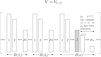
Figure 1. The matrix $V_{i-1}$ and the block $B(\alpha)$ at stage $i$ of the proof. At the $j$th step in processing $V$, the columns $(j+1)$ to $\mu_{\alpha}$ of the block $B(\alpha)$ have been processed to obtain $V^{(j+1)}$. In $V^{(j+1)}$, the $j$th column is processed to obtain $V^{(j)}$.

We will now process the columns of $B(\alpha)$ starting from the last column to the first in $V$; it will help the reader to note that the columns will be counted from $1$ to $\mu_{\alpha}$. Suppose we have already processed the columns of $B(\alpha)$ from $\mu_{\alpha}$ down to $(j+1)$ in $V$; let $V^{(j+1)}$ be the resulting matrix; initially, define $V^{(\mu_{\alpha}+1)}{\color[rgb]{1,0,0}\mathop{\mbox{\rm:=}}}V$. For $\beta_{\ell}$, $\ell=1,\ldots,k$, define

(21) $$r_{\ell}{\color[rgb]{1,0,0}\mathop{\mbox{\rm:=}}}\begin{cases}\mu_{\ell}&\text{ if $w_{\ell}$ is divisible by $\mu_{\ell}$,}\\ (w_{\ell}\text{ mod }\mu_{\ell})&\text{ otherwise}.\end{cases}$$

We inductively claim the following relation for $j\leq\mu_{\alpha}$:

(22) $$\det(V)=\det(V^{(j+1)})\prod_{\kappa=j+1}^{\mu_{\alpha}}\prod_{\ell\in S_{\kappa}}(\beta_{\ell}-\alpha)^{(\kappa-j-1)\mu_{\ell}+r_{\ell}}.$$

The proof is by reverse induction on decreasing values of $j$; the base case trivially holds for $j=\mu_{\alpha}$, since the product vanishes and $V=V^{(\mu_{\alpha}+1)}$ by choice.

To complete the inductive claim (22), we have to obtain the following terms from the $j$th column in $B(\alpha)$:

1. the residue terms $(\beta_{\ell}-\alpha)^{r_{\ell}}$, for each index $\ell\in S_{j}$, and

2. a factor of $(\beta_{\ell}-\alpha)^{\mu_{\ell}}$ for all the indices $\ell\in S_{\kappa}$, where $\kappa>j$.

This is done by taking a suitable partial derivative of the finite difference. Let

(23) $$N_{j}{\color[rgb]{1,0,0}\mathop{\mbox{\rm:=}}}|\cup_{\kappa=j}^{\mu_{\alpha}}S_{\kappa}|,$$

that is the total number of indices assigned to column $j$ or greater; clearly $N_{j}\leq k$. We will introduce $N_{j}$ variables for each of these indices, and a variable $y_{0}$ for $\alpha$. Note that the $j$th column of the block $B(\alpha)$ in $V^{(j+1)}$ is obtained by substituting $z=\alpha$ in $v_{j-1}(z)$ given in (5). The $m$th entry of this column, for $m=1,\ldots,n$, is

(24) $${m-1\choose j-1}z^{m-j}=\frac{(z^{m-1})^{(j-1)}}{(j-1)!}.$$

Define $f_{m}(z){\color[rgb]{1,0,0}\mathop{\mbox{\rm:=}}}z^{m-1}$, and consider the finite difference

$$f_{m}[y_{0},y_{1},\ldots,y_{N_{j}}],$$

where the $y_{\ell}$’s are variables. Since the order of $y_{i}$’s in (16) does not matter, we can assume without loss of generality that $S_{j}=\left\{1,\ldots,|S_{j}|\right\}$, the indices in $S_{j+1}$ are the next $|S_{j+1}|$ numbers, and so on $S_{\mu_{\alpha}}$ is the last $|S_{\mu_{\alpha}}$ numbers smaller than $N_{j}$; thus the sets $S_{\kappa}$, for $\kappa=j,\ldots,\mu_{\alpha}$, form a partition of the set $\left\{1,\ldots,N_{j}\right\}$. Further define

(25) $$i_{0}{\color[rgb]{1,0,0}\mathop{\mbox{\rm:=}}}j-1,\;i_{\ell}{\color[rgb]{1,0,0}\mathop{\mbox{\rm:=}}}r_{\ell}-1,$$

for $\ell=1,\ldots,|S_{j}|$, and

(26) $$i_{\ell}=\mu_{\ell}-1,$$

for $\ell=|S_{j}|+1,\ldots,N_{j}$. Then we replace the $m$th entry of the $j$th column $v_{j-1}(\alpha)$ in the matrix $V^{(j+1)}$ by

(27) $$f_{m}^{(i_{0},\ldots,i_{N_{j}})}[y_{0},y_{1},\ldots,y_{N_{j}}]$$

and substitute $y_{0}{\color[rgb]{1,0,0}\mathop{\mbox{\rm:=}}}\alpha$, and $y_{\ell}{\color[rgb]{1,0,0}\mathop{\mbox{\rm:=}}}\beta_{\ell}$, for $\ell=1,\ldots,N_{j}$.This is done for all the $n$ entries (that is, $m=1,\ldots,n$) in the $j$th column. Let $V^{(j)}$ be the resulting matrix. From Lemma 3.3 we know that the coefficient of $f_{m}^{(i_{0})}(y_{0})$ is

(28) $$\frac{1}{i_{0}!}\prod_{\ell=1}^{N_{j}}\frac{1}{(y_{0}-y_{\ell})^{i_{\ell}+1}}=\frac{1}{(j-1)!}\prod_{\kappa=j}^{\mu_{\alpha}}\prod_{\ell\in S_{\kappa}}\frac{1}{(\alpha-\beta_{\ell})^{i_{\ell}+1}},$$

which is same for all $m=1,\ldots,n$. Therefore, the replacement of the entries of the $j$th column in the matrix $V^{(j+1)}$ by (27), for $m=1,\ldots,n$, is tantamount to obtaining the matrix $V^{(j)}$ from $V^{(j+1)}$ by replacing the $j$th column of $V^{(j+1)}$ by a linear combination of its other columns and a scaled version of the $j$th column, where the scaling factor is the product term in (28); the $1/(j-1)!$ is not part of the scaling as it already occurs in all the entries of the column (see (24)). In terms of the determinant, we obtain the following relation:

$$\det(V^{(j+1)}) =\det(V^{(j)})\prod_{\kappa=j}^{\mu_{\alpha}}\prod_{\ell\in S_{\kappa}}(\beta_{\ell}-\alpha)^{i_{\ell}+1}$$

$$=\det(V^{(j)})\prod_{\ell\in S_{j}}(\beta_{\ell}-\alpha)^{r_{\ell}}\prod_{\kappa=j+1}^{\mu_{\alpha}}\prod_{\ell\in S_{\kappa}}(\beta_{\ell}-\alpha)^{\mu_{\ell}}.$$

Substituting this in (22), we have the desired inductive relation:

$$\det(V)=\det(V^{(j)})\prod_{\kappa=j}^{\mu_{\alpha}}\prod_{\ell\in S_{\kappa}}(\beta_{\ell}-\alpha)^{(\kappa-j)\mu_{\ell}+r_{\ell}}.$$

We stop when $j=1$, to get

$$\det(V)=\det(V^{(1)})\prod_{\kappa=1}^{\mu_{\alpha}}\prod_{\ell\in S_{\kappa}}(\beta_{\ell}-\alpha)^{(\kappa-1)\mu_{\ell}+r_{\ell}}.$$

But recall from (20) that for an index $\ell\in S_{\kappa}$, we have $\left\lceil{w_{\ell}/\mu_{\ell}}\right\rceil=\kappa$. Furthermore, from (21) it follows that $w_{\ell}=(\kappa-1)\mu_{\ell}+r_{\ell}$. Since $\cup_{\kappa=1}^{\mu_{\alpha}}S_{\kappa}=[k]$, we have accounted for all the $\beta_{\ell}$’s, and so the equation above is the same as

$$\det(V) =\det(V^{(1)})\prod_{\ell=1}^{k}(\beta_{\ell}-\alpha)^{w_{\ell}}$$

$$=\det(V^{(1)})\prod_{\alpha_{j}\in\text{In}(\alpha_{i})}(\alpha_{j}-\alpha)^{w(\alpha_{j},\alpha_{i})}.$$

Defining $V_{i}{\color[rgb]{1,0,0}\mathop{\mbox{\rm:=}}}V^{(1)}$ and recalling that $V=V_{i-1}$, we complete the proof of the inductive claim (19). Applying the claim for $i=1$ to $r$, and making appropriate substitutions, we get the desired relation (29).

(29) $$\det(V_{0})=\det(V_{r})\prod_{i=1}^{r}\prod_{\alpha_{j}\in\text{In}(\alpha_{i})}(\alpha_{i}-\alpha_{j})^{w(\alpha_{j},\alpha_{i})},$$

where $V_{0}=V({\boldsymbol{\alpha}};{\boldsymbol{\mu}})$ (see (18)) The absolute value of the product on the right-hand side is the value that we need to lower bound; we know the determinant on the left-hand side from Proposition 2.1, so all that remains is to derive an upper bound on $|\det(V_{r})|$. We will use Hadamard’s inequality for this purpose, which requires us to derive an upper bound on the two-norms of the columns of the matrix $V_{r}$. Let $V_{r}(\alpha_{i};j)$ denote the $j$th column of the block of columns $V_{r}(\alpha_{i})$ corresponding to $B(\alpha_{i})$ in $V_{0}$; note that $V_{r}(\alpha_{i})$ may be the same as $B(\alpha_{i})$ (this happens, for instance, when there are no edges incident on $\alpha_{i}$ in $\mathcal{G}$). In what follows, we derive an upper bound on $\|V_{r}(\alpha_{i};j)\|_{2}$.

Recall the definition of $N_{j}$ from (23), and that $\mu_{i}$ is the size of the block $B(\alpha_{i})$. For convenience again, let the sets $S_{j},S_{j+1},\ldots,S_{\mu_{i}}\subseteq\text{In}(\alpha_{i})$ be indexed such that $S_{j}=\left\{1,\ldots,|S_{j}|\right\}$, the next $|S_{j+1}|$ numbers are in $S_{j+1}$ and so on until $S_{\mu_{i}}$ is the last $|S_{\mu_{i}}|$ numbers smaller than $N_{j}$; thus these sets form a partition of the set $\left\{1,\ldots,N_{j}\right\}$. Now the $m$th entry in the column $V_{r}(\alpha_{i};j)$ is (27). From (17), we have the following bound on the absolute value of (27) after substituting $n{\color[rgb]{1,0,0}\mathop{\mbox{\rm:=}}}N_{j}+1$, $y_{0}=\alpha_{0}{\color[rgb]{1,0,0}\mathop{\mbox{\rm:=}}}\alpha_{i}$, $y_{\ell}{\color[rgb]{1,0,0}\mathop{\mbox{\rm:=}}}\alpha_{\ell}$, $\ell=1,\ldots,N_{j}$, and the indices $i_{\ell}$’s are defined as in (25) and (26):

$${\sum}_{\begin{subarray}{c}(t_{0},t_{1},\ldots,t_{N_{j}})\in{\mathbb{Z}}_{\geq 0}^{N_{j}+1}\\ t_{0}+t_{1}+\cdots+t_{N_{j}}=m-1-N_{j}\end{subarray}}\prod_{\ell=0}^{N_{j}}{t_{\ell}\choose i_{\ell}}\left\lvert\alpha_{\ell}\right\rvert^{t_{\ell}-i_{\ell}}.$$

Since $\alpha_{1},\ldots,\alpha_{N_{j}}$ have edges directed to $\alpha_{i}$, their absolute values are smaller than $|\alpha_{i}|$. Therefore, the quantity above is upper bounded by

$${\sum}_{\begin{subarray}{c}(t_{0},t_{1},\ldots,t_{N_{j}})\in{\mathbb{Z}}_{\geq 0}^{N_{j}+1}\\ t_{0}+t_{1}+\cdots+t_{N_{j}}=m-1-N_{j}\end{subarray}}\prod_{\ell=0}^{N_{j}}{t_{\ell}\choose i_{\ell}}\left\lvert\alpha_{i}\right\rvert^{m-1-N_{j}-i_{\ell}},$$

which is equal to

(30) $$\left\lvert\alpha_{i}\right\rvert^{m-1-N_{j}-\sum_{\ell=0}^{N_{j}}i_{\ell}}{\sum}_{\begin{subarray}{c}(t_{0},t_{1},\ldots,t_{N_{j}})\in{\mathbb{Z}}_{\geq 0}^{N_{j}+1}\\ t_{0}+t_{1}+\cdots+t_{N_{j}}=m-1-N_{j}\end{subarray}}\prod_{\ell=0}^{N_{j}}{t_{\ell}\choose i_{\ell}}.$$

Define

(31) $$M_{j}{\color[rgb]{1,0,0}\mathop{\mbox{\rm:=}}}N_{j}+\sum_{\ell=0}^{N_{j}}i_{\ell}=N_{j}+j-1+\sum_{\ell=1}^{N_{j}}i_{\ell},$$

where the second equality follows from the fact that $i_{0}=j-1$ (see the definition in (25)). The binomial coefficients ${t_{\ell}\choose i_{\ell}}$ vanish for $t_{\ell}<i_{\ell}$, so we can assume that $t_{\ell}\geq i_{\ell}$. If $j_{\ell}{\color[rgb]{1,0,0}\mathop{\mbox{\rm:=}}}t_{\ell}-i_{\ell}$, then

$$\sum_{\ell=0}^{N_{j}}t_{\ell}=\sum_{\ell=0}^{N_{j}}i_{\ell}+\sum_{\ell=0}^{N_{j}}j_{\ell},$$

and so the constraint $\sum_{\ell=0}^{N_{j}}t_{\ell}=m-1-N_{j}$ is equivalent to

$$\sum_{\ell=0}^{N_{j}}j_{\ell}=m-1-N_{j}-\sum_{\ell=0}^{N_{j}}=m-1-M_{j}$$

where the last step follows from the definition of $M_{j}$ (31). Changing the indices from $t_{\ell}$ to $j_{\ell}$ in (30), we get the following bound the $m$th entry of $V_{r}(\alpha_{i};j)$:

(32) $$\left\lvert\alpha_{i}\right\rvert^{m-1-M_{j}}{\sum}_{\begin{subarray}{c}(j_{0},j_{1},\ldots,j_{N_{j}})\in{\mathbb{Z}}_{\geq 0}^{N_{j}+1}\\ j_{0}+j_{1}+\cdots+j_{N_{j}}=m-1-M_{j}\end{subarray}}\prod_{\ell=0}^{N_{j}}{i_{\ell}+j_{\ell}\choose i_{\ell}}.$$

We next derive a closed form for the summation term above.

Consider the generating function

$$\sum_{t_{\ell}\geq i_{\ell}}{t_{\ell}\choose i_{\ell}}x^{t_{\ell}-i_{\ell}}=\sum_{j_{\ell}\geq 0}{i_{\ell}+j_{\ell}\choose j_{\ell}}x^{j_{\ell}}=(1-x)^{-(i_{\ell}+1)}$$

for a given $\ell$. Taking the product of these for different choices of $\ell$, it follows that the summation term in the right-hand side of (32) is the coefficient of $x^{m-1-M_{j}}$ in the generating function

$$(1-x)^{-\sum_{\ell=0}^{N_{j}}(i_{\ell}+1)}=(1-x)^{-(M_{j}+1)}$$

which is

$${m-1\choose M_{j}}.$$

This implies that (32) is equal to $|\alpha_{i}|^{m-1-M_{j}}{m-1\choose M_{j}}$.

From the argument in the preceding paragraph, it follows that in the matrix $V_{r}$ the two-norm of the $j$th column, in the block of columns corresponding to $B(\alpha_{i})$, is

$$\|V_{r}(\alpha_{i};j)\|_{2}\leq\left({\sum_{m=1}^{n}|\alpha_{i}|^{2(m-1-M_{j})}{m-1\choose M_{j}}^{2}}\right)^{1/2}.$$

Since for $m-1\leq M_{j}$ the binomial term vanishes, we can start the summation from $M_{j}$ onwards to obtain the following equivalent form

$$\|V_{r}(\alpha_{i};j)\|_{2}\leq\left({\sum_{m=M_{j}}^{n-1}|\alpha_{i}|^{2(m-M_{j})}{m\choose M_{j}}^{2}}\right)^{1/2}.$$

Substituting $|\alpha_{i}|$ by

(33) $$\max_{1}|\alpha_{i}|{\color[rgb]{1,0,0}\mathop{\mbox{\rm:=}}}\max\left\{1,|\alpha_{i}|\right\}$$

and pulling out its largest power from the summation we have the following upper bound on the two-norm

$$\|V_{r}(\alpha_{i};j)\|_{2}\leq\max_{1}|\alpha_{i}|^{(n-1-M_{j})}\left({\sum_{m=M_{j}}^{n-1}{m\choose M_{j}}^{2}}\right)^{1/2}.$$

Using the upper bound from (Escorcielo and Perrucci, 2017, Lemma 7) on the summation term above, we get the following inequality

$$\|V_{r}(\alpha_{i};j)\|_{2}\leq\max_{1}|\alpha_{i}|^{(n-1-M_{j})}\left({\frac{n}{\sqrt{3}}}\right)^{M_{j}}\sqrt{n}.$$

Taking the product of these quantities for $j=1,\ldots,\mu_{i}$, we get the following upper bound on the product of the two-norms of the columns in the block $V_{r}(\alpha_{i})$ in $V_{r}$:

(34) $$\prod_{j=1}^{\mu_{i}}\|V_{r}(\alpha_{i};j)\|_{2}\leq\max_{1}|\alpha_{i}|^{\sum_{j=1}^{\mu_{i}}(n-1-M_{j})}\left({\frac{n}{\sqrt{3}}}\right)^{\sum_{j=1}^{\mu_{i}}M_{j}}{n}^{\mu_{i}/2}.$$

Let us understand the term $\sum_{j=1}^{\mu_{i}}M_{j}$.

Lemma 4.1.

For a vertex $\alpha_{i}$ in the directed acyclic graph $\mathcal{G}$, define

(35) $$w_{i}{\color[rgb]{1,0,0}\mathop{\mbox{\rm:=}}}\sum_{\alpha_{\ell}\in\text{In}(\alpha_{i})}w(\alpha_{\ell},\alpha_{i}),$$

that is, the sum of the weights of all edges incident on $\alpha_{i}$. Then

$$\sum_{j=1}^{\mu_{i}}M_{j}={\mu_{i}\choose 2}+w_{i}.$$

Proof.

Recall the definition of the sets $S_{j}$, from (20), and the definition of $M_{j}$, from (31). Given a $j$, and $\ell\in S_{j}$, $i_{\ell}=r_{\ell}-1$ from (25); for $\ell\in S_{\kappa}$, where $\kappa=j+1,\ldots,\mu_{i}$, $i_{\ell}=\mu_{\ell}-1$. Therefore, we can rewrite (31) as

$$M_{j} =N_{j}+j-1+\sum_{\ell\in S_{j}}(r_{\ell}-1)+\sum_{\ell\in\cup_{\kappa>j}S_{\kappa}}(\mu_{\ell}-1)$$

$$=j-1+\sum_{\ell\in S_{j}}r_{\ell}+\sum_{\ell\in\cup_{\kappa>j}S_{\kappa}}\mu_{\ell}.$$

The sum $\sum_{j}\sum_{\ell\in S_{j}}r_{\ell}$ is the sum of the residue terms over all indices in $\cup_{j=1}^{\mu_{i}}S_{j}$. Now consider the sum

$$\sum_{j=1}^{\mu_{i}}\sum_{\ell\in\cup_{\kappa>j}S_{\kappa}}\mu_{\ell}.$$

For two indices $j<\kappa$, the summation over $j$ contributes an $\mu_{\ell}$ for every $\ell\in S_{\kappa}$. Therefore,

$$\sum_{j=1}^{\mu_{i}}\left({\sum_{\ell\in S_{j}}r_{\ell}+\sum_{\ell\in\cup_{\kappa>j}S_{\kappa}}\mu_{\ell}}\right)=w_{i}$$

∎

Substituting the result in the lemma above into (34), we get the following upper bound on the two-norms of the columns in $V_{r}(\alpha_{i})$

$$\prod_{j=1}^{\mu_{i}}\|V_{r}(\alpha_{i};j)\|_{2}\leq\max_{1}|\alpha_{i}|^{(n-1)\mu_{i}-{\mu_{i}\choose 2}-w_{i}}\left({\frac{n}{\sqrt{3}}}\right)^{{\mu_{i}\choose 2}+w_{i}}{n}^{\mu_{i}/2}.$$

Taking the product of this bound for $i=1,\ldots,r$, along with Hadamard’s inequality, gives us the following upper bound

(36) $$|\det(V_{r})|\leq\prod_{i=1}^{r}\left({\max_{1}|\alpha_{i}|^{(n-1)\mu_{i}-{\mu_{i}\choose 2}-w_{i}}\left({\frac{n}{\sqrt{3}}}\right)^{{\mu_{i}\choose 2}+w_{i}}}\right){n}^{n/2}.$$

where we use the fact that $n=\sum_{i=1}^{r}\mu_{i}$. The term

$$(n-1)\mu_{i}-{\mu_{i}\choose 2}-w_{i}=\sum_{j=1;j\neq i}^{r}\mu_{i}\mu_{j}-w_{i}+{\mu_{i}\choose 2}<\sum_{\begin{subarray}{c}j=1\\ j\neq i\end{subarray}}^{r}\mu_{i}\mu_{j}-w_{i}+\mu_{i}^{2}.$$

If ${\boldsymbol{\mu}}$ be the column vector of all $\mu_{i}$’s, and $A_{w}$ be the adjacency matrix with the $(i,j)$th entry as the weight $w(\alpha_{i},\alpha_{j})$ of the corresponding edge $(\alpha_{i},\alpha_{j})$, then the last term in the inequality above is the one-norm of the $i$th row of the matrix ${\boldsymbol{\mu}}{\boldsymbol{\mu}}^{t}-A_{w}$. Since the $\infty$-norm of the matrix $\|{\boldsymbol{\mu}}{\boldsymbol{\mu}}^{t}-A_{w}\|_{\infty}$ is the maximum over all the row-sums, we have

$$(n-1)\mu_{i}-{\mu_{i}\choose 2}-w_{i}\leq\|{\boldsymbol{\mu}}{\boldsymbol{\mu}}^{t}-A_{w}\|_{\infty}.$$

As for the term

$$\sum_{i=1}^{r}\left({{\mu_{i}\choose 2}+w_{i}}\right)=\sum_{i=1}^{r}{\mu_{i}\choose 2}+w(E),$$

where $w(E)$ is defined in (12). Substituting these bounds in (36), we obtain the following upper bound

(37) $$|\det(V_{r})|\leq M({\boldsymbol{\alpha}})^{\|{\boldsymbol{\mu}}{\boldsymbol{\mu}}^{t}-A_{w}\|_{\infty}}\left({\frac{n}{\sqrt{3}}}\right)^{\sum_{i}{\mu_{i}\choose 2}+w(E)}{n}^{n/2}.$$

Substituting this upper bound in (29) and moving it to the denominator in the left-hand side completes the proof of Theorem 3.2.

4.1. Choosing the best matrix

Theorem 3.2 leaves open the choice of the potentials $\mu_{i}\in{\mathbb{N}}$, $i=1,\ldots,r$. Our aim here is to find the best possible choice of $\mu_{i}$’s satisfying the edge constraints $w(\alpha_{i},\alpha_{j})\leq\mu_{i}\mu_{j}$ and at the same time minimizing $\|{\boldsymbol{\mu}}{\boldsymbol{\mu}}^{t}-A_{w}\|_{\infty}$. For example, if all the weights are one then it is clear that $\mu_{i}=1$, for $i=1,\ldots,r$, is the best possible assignment. In which case,

$$V({\boldsymbol{\alpha}};{\boldsymbol{\mu}})=V({\boldsymbol{\alpha}}),\;\|{\boldsymbol{\mu}}{\boldsymbol{\mu}}^{t}-A_{w}\|_{\infty}\leq(r-1),\;n=r,\;w(E)=|E|$$

and so Theorem 3.2 matches the bound given in Proposition 3.1.

Consider the relaxed version of the problem where $\mu_{i}$’s are positive reals; it is clear that rounding them up to the nearest integer would give a valid solution (though not an optimum solution) to the problem over the positive integers. Then the optimization problem is to minimize $\|{\boldsymbol{\mu}}{\boldsymbol{\mu}}^{t}-A_{w}\|_{\infty}$ such that

$${\boldsymbol{\mu}}{\boldsymbol{\mu}}^{t}\geq A_{w}$$

where ‘$\geq$’ here means entry wise; note that the non-edge constraints are trivially satisfied since no $\mu_{i}$ is ever assigned to zero. Since $A_{w}$ is non-negative, we know from the Perron-Frobenius theory (Horn and Johnson, 1991) that the spectrum of $A_{w}$ is an eigenvalue $\rho(A_{w})$ of $A_{w}$. Moreover, as $A_{w}$ is symmetric it can be orthogonally diagonalized, i.e., $A_{w}=Q\Lambda Q^{t}$, where $Q$ is the $r\times r$ orthogonal matrix whose columns ${\boldsymbol{q}}_{k}$, $k=1,\ldots,r$, are the eigenvectors of $A_{w}$ and $\Lambda$ is a diagonal matrix that has the corresponding eigenvalues of $A_{w}$. Another way to express the relation is that $A_{w}$ is the sum of some rank one matrices obtained by its eigenvectors, i.e.,

$$A_{w}=\sum_{k=1}^{r}\lambda_{k}{\boldsymbol{q}}_{k}{\boldsymbol{q}}_{k}^{t}.$$

We can also assume that the $\|{\boldsymbol{q}}_{k}\|_{2}=1$ for $k=1,\ldots,r$. Combined with the equation above it follows that the $(i,j)$-th entry of $A_{w}$

$$w(\alpha_{i},\alpha_{j})=\sum_{k=1}^{r}\lambda_{k}{\boldsymbol{q}}_{k,i}{\boldsymbol{q}}_{k,j}.$$

Since by assumption $\|{\boldsymbol{q}}_{k}\|_{2}=1$, taking absolute values we get

$$w(\alpha_{i},\alpha_{j})\leq\sum_{k=1}^{r}|\lambda_{k}|=\|A_{w}\|_{\star},$$

where $\|A_{w}\|_{\star}$ is the nuclear norm of $A_{w}$. Therefore, we can take ${\boldsymbol{\mu}}$ in Theorem 3.2 as the vector

(38) $${\boldsymbol{\mu}}{\color[rgb]{1,0,0}\mathop{\mbox{\rm:=}}}\left\lceil{\sqrt{\|A_{w}\|_{\star}}}\right\rceil\overbrace{(1,1,\ldots,1)}^{r},$$

which implies that

$$n=r\left\lceil{\sqrt{\|A_{w}\|_{\star}}}\right\rceil$$

in the theorem. The error in the approximation can be shown to be bounded by

$$\|{\boldsymbol{\mu}}{\boldsymbol{\mu}}^{t}-A_{w}\|_{\infty} \leq 2r\|A_{w}\|_{\star},$$

and

$$\sum_{i}{\mu_{i}\choose 2}\leq\frac{3r\|A_{w}\|_{\star}}{2},$$

where in the last inequality we use the observation that as $A_{w}$ has entries in ${\mathbb{Z}}_{\geq 0}$, its spectrum is greater than one, and hence $\|A_{w}\|_{\star}\geq 1$. By making these substitutions in Theorem 3.2, we obtain the result, namely (4), mentioned in Section 1.

5. Conclusion and Future Work

Our derivation using the confluent Vandermonde matrix to get the desired weights in the exponents has the advantage of optimizing over the various choices of the matrix. We have given a first attempt at exploiting this choice. Whereas rank-one approximations to matrices are well studied (Friedland, 2013), the challenge in our context is to derive a symmetric rank-one matrix that also dominates $A_{w}$.

One would also like to derive a lower bound on the absolute value of $\det(V({\boldsymbol{\alpha}};{\boldsymbol{\mu}}))$ in terms of the polynomial $f$, to get a more direct comparison with the earlier results. Perhaps an algorithm to compute the determinant from the coefficients would also be interesting; a related recent result is an algorithm to compute the $D^{+}(f)$-root function defined as $\prod_{1\leq i<j\leq r}(\alpha_{i}-\alpha_{j})^{m_{i}+m_{j}}$, i.e., $G$ is the complete graph on the roots and the weight of an edge is the sum of the multiplicity of its vertices (Yang and Yap, 2020). Similar to (Emiris et al., 2019), one would like to derive weighted version of the results for the more general setting of polynomial systems.

References

• (1)
• Batra and Sharma (2019) Prashant Batra and Vikram Sharma. 2019. Complexity of a Root Clustering Algorithm. CoRR abs/1912.02820 (2019). arXiv:1912.02820 http://arxiv.org/abs/1912.02820
• Becker et al. (2018) Ruben Becker, Michael Sagraloff, Vikram Sharma, and Chee Yap. 2018. A near-optimal subdivision algorithm for complex root isolation based on the Pellet test and Newton iteration. Journal of Symbolic Computation 86 (2018), 51 – 96. https://doi.org/10.1016/j.jsc.2017.03.009
• Davenport (1985) James H. Davenport. 1985. Computer algebra for Cylindrical Algebraic Decomposition. Tech. Rep. The Royal Inst. of Technology, Dept. of Numerical Analysis and Computing Science, S-100 44, Stockholm, Sweden. Reprinted as Tech. Report 88-10 , School of Mathematical Sci., U. of Bath, Claverton Down, Bath BA2 7AY, England. URL http://www.bath.ac.uk/~masjhd/TRITA.pdf.
• Eigenwillig (2008) Arno Eigenwillig. 2008. Real Root Isolation for Exact and Approximate Polynomials Using Descartes’ Rule of Signs. Ph.D. Thesis. University of Saarland, Saarbruecken, Germany.
• Eigenwillig et al. (2006) Arno Eigenwillig, Vikram Sharma, and Chee Yap. 2006. Almost Tight Complexity Bounds for the Descartes Method. In Proc. of the 31st Intl. Symp. on Symbolic and Algebraic Computation. 71–78. Genova, Italy. Jul 9-12, 2006.
• Emiris et al. (2019) Ioannis Emiris, Bernard Mourrain, and Elias Tsigaridas. 2019. Separation bounds for polynomial systems. Journal of Symbolic Computation (2019). https://doi.org/10.1016/j.jsc.2019.07.001
• Escorcielo and Perrucci (2017) Paula Escorcielo and Daniel Perrucci. 2017. On the Davenport-Mahler bound. J. Complexity 41 (2017), 72–81. https://doi.org/10.1016/j.jco.2016.12.001
• Friedland (2013) Shmuel Friedland. 2013. Best rank one approximation of real symmetric tensors can be chosen symmetric. Frontiers of Mathematics in China 8 (2013), 19–40. https://doi.org/10.1007/s11464-012-0262-x.
• Horn and Johnson (1991) R. Horn and C. Johnson. 1991. Topics in Matrix Analysis. Cambridge University Press, Cambridge.
• Kobel and Sagraloff (2015) Alexander Kobel and Michael Sagraloff. 2015. On the complexity of computing with planar algebraic curves. J. Complexity 31, 2 (2015), 206–236. https://doi.org/10.1016/j.jco.2014.08.002
• Mignotte (1992) Maurice Mignotte. 1992. Mathematics for Computer Algebra. Springer-Verlag, Berlin.
• Mignotte (1995) Maurice Mignotte. 1995. On the Distance Between the Roots of a Polynomial. Applicable Algebra in Engineering, Commun., and Comput. 6 (1995), 327–332.
• Pan (2002) Victor Y. Pan. 2002. Univariate polynomials: Nearly optimal algorithms for numerical factorization and root-finding. Journal of Symbolic Computation 33, 5 (2002), 701–733.
• Yang and Yap (2020) Jing Yang and Chee K. Yap. 2020. On mu-Symmetric Polynomials. arXiv:cs.SC/2001.07403