Controlled quantum state transfer in $XX$ spin chains at the Quantum Speed Limit

Abstract

The Quantum Speed Limit can be found in many different situations, in particular in the propagation of information through quantum spin chains. In homogeneous chains it implies that taking information from one extreme of the chain to the other will take a time $O(N/2)$, where $N$ is the chain length. Using Optimal Control Theory we design control pulses that achieve near perfect population transfer between the extremes of the chain at times on the order of $N/2$, or larger, depending on which features of the transfer process are to be studied. Our results show that the control pulses that govern the dynamical behaviour of chains with different lengths are closely related, that larger control times imply more complicated control pulses than those found at times on the order of $N/2$ and also larger driving energies. The pulses were constructed for control schemes involving one or two actuators in chains with exchange couplings without static disorder. Our results also show that the two actuator scheme is considerably more robust against the presence of static disorder than the scheme that uses just a single one.

I Introduction

The transfer, or transmission, of quantum states in different communication channels has been touted as a task of paramount importance to routinely implement Quantum Information Processing (QIP) and Technologies. Since the paper of Sougato Bose in 2003 Bose2003 the area has grow enormously and the understanding of the field has been collected in books Nikolopoulos2015 and other excellent reviews Bose-review . Also from the beginning, it was understood that the severe restrictions imposed by the fragility of the quantum states to be transferred required perfect or near perfect quantum transmission so the errors do not spoil the state for further use after it has been transmitted.

The transmission channel is constructed from copies of a given physical system. The copies are spatially distributed along a line or in other spatial distributions Kostak2007 and might or might not interact with a surrounding environment. Many different physical systems have been considered as the basic unit of the communication channel, quantum dots quantum-dot-chain , superconductor qubits Li2018 , nuclear spins nuclear-spin-chain , cold atoms or ions trapped in arrays Loft2011 ; Banchi2011prl or coupled waveguides Chapman2016 . Anyway, most theoretical studies focus on Heisenberg or $XY$ spin chain models since these models captures the basic physical traits that are of interest. In the case of quantum dots chains most theoretical studies deal with the Hubbard model Hawrylak although other approaches are feasible Coden2019 .

In models without environment, i.e. with unitary dynamics, there are two main approaches to achieve perfect or near perfect sate transfer. In the simpler approach the Hamiltonian unitary dynamics takes the state to be transferred from one extreme of the spin chain to the other and the spin chain Hamiltonian is time-independent. Several possibilities have been studied, for example, chains that achieve perfect transmission by engineering all the spin couplings to special values Christandl2004 ; Christandl2005 ; Yung2006 , conclusive and perfect transmission using to parallel spin chains Burgarth2005 ; Burgarth2005b , boundary controlled spin chains Zwick1 ; Zwick2 ; Zwick3 , optimal dynamics Banchi2010 ; Banchi2011 , and so on. The second approach assumes that the system will be driven by control fields, so the dynamical behavior is governed by the free Hamiltonian and a number of external fields. Both approaches share some features, usually the dynamics is confined to some sub-space of the whole Hilbert space, most commonly a sub-space with fixed number of excitations or magnetization. This assumption reduces drastically the size of the computational problem and makes feasible to study systems with static disorder.

Quantum spin chains of different kinds are controllable in the whole Hilbert space Jurdjevic1972 ; Ramakrishna1995 ; Burgarth2009 and in sub-spaces of fixed magnetization Wang2016 even with very few actuators, moreover Heisenberg spin chains are controllable with just a single actuator. There are numerous papers dealing with the controllability of these models using an external magnetic field applied to the first spin, i.e. the spin where the initial state is prepared to be transmitted. Actually, besides the transmission of quantum states there are other quantum entangling gates that can be controlled along a spin chain Burgarth2010 . The preparation of particular target states has also been considered Stefanatos2019 ; Watanabe2010 , as well as the possibility of controlling the state transfer applying fields to all the sites Gong2007 ; Murphy2010 . Finally, it is important to mention some advances in the last five years in the field of Scanning Tunnel microscopy (STM). In these years we could see that Paramagnetic Electron Resonance (EPR) implemented using STM bauman2015 permits one to drive the electronic and nuclear spins of individual atoms on surfaces, as well as artificially created structures, such as dimers prr6 ; prr9 . In addition, STM technique allows to build longer chainsbryant2015 ; spinelli2014 that can be used for control tasks by implementing protocols through STM-EPR.

The logic behind a reduced number of control fields, and that they are applied to the extremes of the chain, is based on what can be feasible on actual implementations, where each control field could add new sources of errors and the application of an external field to a single element of a truly nano scale device is troublesome at least, in particular it is located in the middle of other elements alike.

Inspired by control techniques typical of Nuclear Magnetic Resonance, the design of control pulses based on trains of square pulses of varying length in time has been intensely studied in Heisenberg spin chains Wang2010 ; Heule2010 . In these studies the strength of the magnetic field applied to the first site of the chain is constant during an interval and different optimization procedures are used to determine the length of the interval and the strength of the field. As is common in studies involving Optimal Control Theory the control time is fixed a priori, in the case of a single control field this time has been chosen on the order of $N^{2}$ Wang2016 ; Burgarth2010 ; Poggi2016 , where $N$ is the number of spins in the chain, but for more involved control algorithms shorter times, compatible with Quantum Speed Limit can be achieved Murphy2010 .

In this paper we present strategies to control state transfer in $XX$ spin chains that achieve fast transfer times, $O(N)$, with very high fidelities and with smooth pulses that control the coupling between the first pair, or the first and last, pair of spins. Our results show that the shape of the pulses for different chain lengths are closely related, and that the external forcing also shows the effect of the Quantum Speed Limit, restricting the time interval in which it is necessary to achieve the transfer.

The paper is organized as follows. In sec. II, we present the model Hamiltonian for the spin chain with and without static disorder and we analize how to design pulses in order to transfer excitations from the first site to the last one. In sec. III we address the possibility of controlling excitations using the optimal control theory in order to design a one actuator control strategy. Sec IV deals with the possibility of performing control tasks with a slightly different strategy, in this case we use pulses designed for two actuators. In both sections we analize the inclusion of static disorder and the efects in the control strategies. Finally, in Sec V we summarize the conclusions of our work.

II Model Hamiltonian and Optimal Control Theory

II.1 Model Hamiltonian, with and without disorder and dynamics

We consider a spin-$1/2$ chain with interactions between nearest neighbors, described by the Hamiltonian

$$H=-\frac{\hbar}{2}\sum_{i=1}^{N-1}J_{i}\left(\hat{\sigma}_{i}^{x}\hat{\sigma}_{i+1}^{x}+\hat{\sigma}_{i}^{y}\hat{\sigma}_{i+1}^{y}\right)$$ (1)

where $\sigma_{i}$ are the Pauli matrices, $N$ is the chain length and $J_{i}\geq 0$ are the exchange interaction couplings. In this work we set $J_{i}=1$ for $i=2,3,...,N-1$ and $J_{1}=J_{N}=\alpha$.

We have introduced the Hamiltonian of a spin chain without any external perturbation. However, since the perfect engineering of all spin couplings is highly improbable, it results interesting to analyze the performance of different spin-coupling distributions related to imperfect construction of such chains. To study the robustness of the spin chains against perturbations we introduce static random spin-coupling imperfections quantified by $\delta_{i}$

$$J_{i}\rightarrow J_{i}(1+\delta_{i}),$$ (2)

where each $\delta_{i}$ is an independent uniformly distributed random variable in the interval $[-A,A]$, this way of introducing static disorder in quantum spin chains has been analyzed extensively, see references [Zwick2, ; Zwick3, ; Petrosyan2010, ] and references therein. $A$ is a positive real number that characterizes the maximum perturbation strength relative to $J_{i}$. The kind of disorder depends on the particular experimental method used to engineer the spin chains.

For ferromagnetic couplings $J_{i}\geq 0$ the fundamental state is the state without excitations (all the spins down). The Hamiltonian in Eq. (1) commutes with the total magnetization in the $z$ direction, so its is possible to analyze problems restricted to sub-spaces with fixed number of excitations, i.e. fixed magnetization. Following the protocol for quantum state transfer introduced by Bose Bose2003 our analysis will be restricted to the sub-space of one excitation. Moreover, since it has been shown that in this subspace the transfer fidelity averaged over realizations of the disorder, Eq. (2), is a function of the probability amplitude that an excitation in the first site of the chain be transferred to the last site in the next Sections we will focus in the “population” of the last site, as a function of time.

Before proceeding to study particular systems it is worth to consider, once more, which kind of couplings are best suited to be implemented experimentally in order to obtain a chain easily controllable, but without too much coupling engineering. As has been above the engineering of all couplings to the precise values required to obtain perfect transmission as in References Christandl2004 and Christandl2005 is beyond what is feasible. Spin chains with only two modified couplings, with respect to a otherwise homogeneous spin chain, can be tuned to transfer states with high fidelity Banchi2010 ; Zwick1 and are surprisingly robust to static disorder Zwick2 ; Zwick3 , so they seem as a good option as the coupling distribution of choice.

II.2 Optimal control of the state dynamics

For controlling excitations in spin chains, we propose to design a time-dependent pulses able to drive an excitation in the first site of the chain $\Psi(0)=\Psi_{1}$ to an excitation in the last site of the chain $\Psi(T)=\Psi_{N}$, in a given prescribed time $T$ as short as possible to avoid unwanted effects of the environment over the coherence of the system.

We assume that the exchange couplings of the ends of the chain are controled by electric pulses and have a time-dependent shape given by the functions $F(t)$ and $G(t)$ for the first and last coupling respectively. Then, the state $\Psi(t)$ must satisfy the time-dependent Schrödinger equation

$$i\frac{\partial\Psi(t)}{\partial t}=H\Psi(t)=[H_{0}-\hat{h}_{L}F(t)-\hat{h}_{R}G(t)]\Psi(t).$$ (3)

where $H_{0}$ is defined in Eq. 1 and

$$\hat{h}_{L}=\frac{\hbar}{2}\left(\hat{\sigma}_{1}^{x}\hat{\sigma}_{2}^{x}+\hat{\sigma}_{1}^{y}\hat{\sigma}_{2}^{y}\right),\qquad\hat{h}_{R}=\frac{\hbar}{2}\left(\hat{\sigma}_{N-1}^{x}\hat{\sigma}_{N}^{x}+\hat{\sigma}_{N-1}^{y}\hat{\sigma}_{N}^{y}\right).$$ (4)

Optimal control theory (OCT) provides a systematic method to calculate variationaly the optimal pulses, $F_{\rm OCT}(t)$ and $G_{\rm OCT}(t)$, that drives the state of the system from an initial state to an state that maximize the overlap with a prescribed target state $\phi_{T}$. We briefly outline here the theory and some technical details of the method as applied in this work werschnik2007 ; putaja2010 .

The total functional to be extremized is the sum of three terms, $J=J_{1}+J_{2}+J_{3}$. The first functional measures the yield of the control process and is defined by

$$J_{1}[\Psi]=|\langle\Psi(T)|\phi_{F}\rangle|^{2},$$ (5)

where $|\phi_{F}\rangle$ is the “target state”.

The second functional is introduced in order to avoid high energy fields and is defined in term of the fluence (the time-integrated intensity of the field),

$$J_{2}[{\bf\varepsilon}]=-\alpha_{L}\left[\int_{0}^{T}F^{2}(t)dt\right]-\alpha_{R}\left[\int_{0}^{T}G^{2}(t)dt\right],$$ (6)

where $\alpha_{L}$ and $\alpha_{R}$ are time-independent Lagrange multipliers. The last functional $J_{3}$ ensures that the electronic wavefunction evolves according to the time-dependent Schrödinger,

$$J_{3}[{\bf\varepsilon},\Psi,\chi]=-2Im\int_{0}^{T}\left\langle\chi(t)\left|\frac{\partial}{\partial t}-H(t)\right|\Psi(t)\right\rangle$$ (7)

where $\chi(t)$ is a time-dependent Lagrange multiplier. The variation of the total functional with respect to $\Psi(t)$, $F(t)$ and $\chi(t)$ allows us to obtain the desired control equations werschnik2007

$$i\frac{\partial\Psi(t)}{\partial t} = H\Psi(t)\;,\;\Psi(0)=\phi,$$ (8)

$$i\frac{\partial\chi(t)}{\partial t} = H(t)\chi(t),$$ (9)

$$\chi(T) = |\phi_{F}\rangle\langle\phi_{F}|\Psi(T)\rangle,$$ (10)

$$F(t) = -\frac{1}{\alpha_{L}}Im\langle\chi(t)|\hat{h}_{L}|\Psi(t)\rangle,$$ (11)

$$G(t) = -\frac{1}{\alpha_{R}}Im\langle\chi(t)|\hat{h}_{R}|\Psi(t)\rangle.$$ (12)

This set of coupled equations can be solved iteratively.

The solution of the system of coupled control equations can be obtained using several approaches, for example, using the efficient forward-backward propagation scheme developed in Ref. kosloff1989 . The algorithm starts with propagating the state of the system from $|\phi\rangle$ forward in time, using in this “zero” iteration a guess of the pulse fields $F^{(0)}(t)$ and $G^{(0)}(t)$. At the end of this step we obtain the wavefunction $|\Psi^{(0)}(T)\rangle$, which is used to evaluate $|\chi^{(0)}(T)\rangle=|\phi_{F}\rangle\langle\phi_{F}|\Psi^{(0)}(T)\rangle$. The algorithm continues with propagating $|\chi^{(0)}(t)\rangle$ backwards in time. At the end of this backward propagation we know both $\Psi^{(0)}$ and $\chi^{(0)}$ at the same time and we can obtain a first version of the optimized pulses $F^{(1)}(t)$ and $G^{(1)}(t)$. We repeat this operation until the convergence of $J$ is achieved. The values of the Lagrange multipliers $\alpha_{R,L}$ are chosen in order to achieve the desired fluences.

The numerical integration of the forward and backward time evolution was performed using high precision Runge-Kutta algorithms under various initial guesses (e.g., constant, random, monochromatic and a superposition of two harmonic pulses). The resulting optimal pulse and the time evolution under its driving were found to be robust for all these various starting conditions.

Note that if the target state $|\phi_{F}\rangle=\Psi_{N}$, the target probability is also the “transferred population” after the controlled transfer protocol has taken place. From now on we use indistinctly both terms.

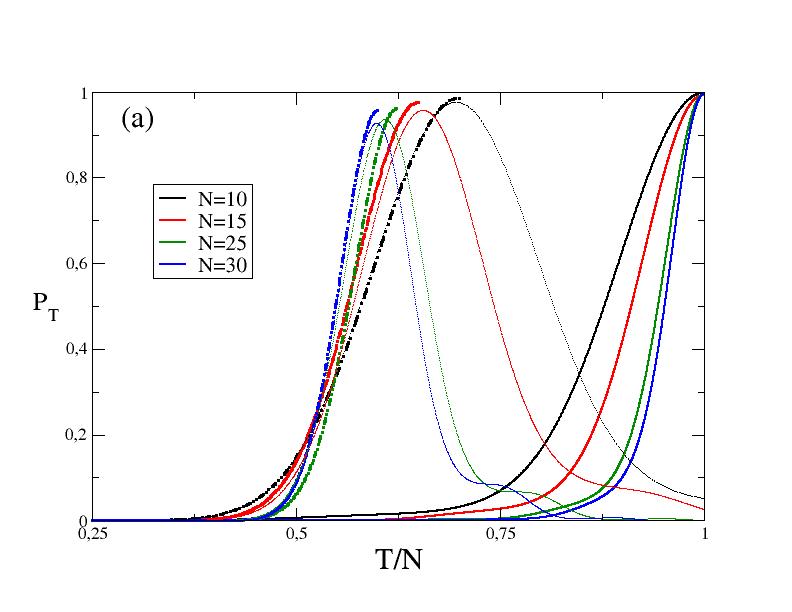
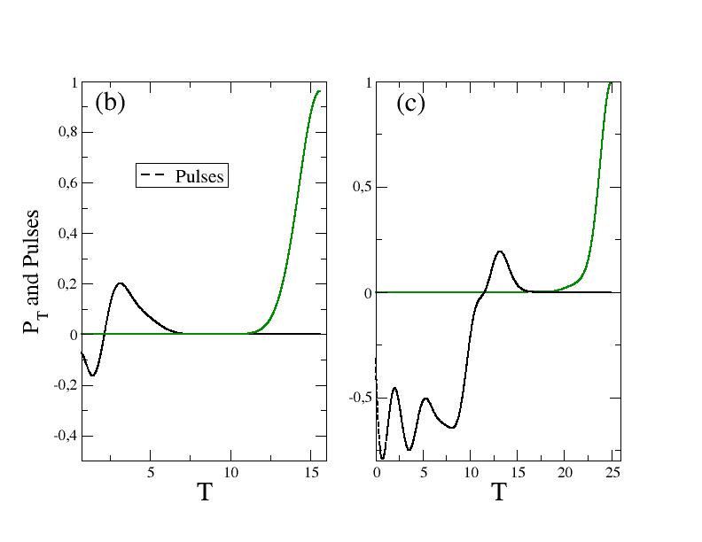
Figure 1: (a) Time evolution of the target probability as a function of the normalized time. Continuous lines show the evolotion for long OCT pulses with $T_{OCT}=N$, dashed lines shows the evoltion for short OCT pulses with $T_{OCT}\simeq T_{Peak}$ and dotted lines show the free evolution. (b) Optimized pulse for short time operation and the target population obtained using this pulse for $N=25$. (c) Optimized pulse for long time operation and the target population obtained using this pulse for $N=25$.

III Control of spin excitation in a $XX$ chain:one actuator

In this section we present results corresponding to the one actuator OCT protocol, as defined in Eq. (3) using $h_{R}=0$. The main objective of the present protocol is to drive an excitation from the first site to the last one through the manipulation of the coupling between the first and second site. As it is known, the free evolution of the excitation, i.e. the evolution without external control, presents a maximum at a certain time which depends upon the size of the chain. In Fig. 1 we compare our OCT results for two different operation times with the corresponding free evolution for various chain sizes. For most of our calculations, as in the calculations performed for Fig. 1, we will consider boundary-controlled XX chains, and we will choose $\alpha$ given by the optimal value obtained for the free evolution Zwick1 .

In Fig. 1 (a) we plot the target probability, i.e. the population at the last site of the chain, for the free evolution in chains with $N=10$, $15$, $25$ and $30$ sites (dotted lines) as a function of a normalized time in terms of the chain size. For instance, the maximum probability for $N=10$ is $P_{Free}(T_{peak})=0.976$ at $T_{peak}\simeq 7a.u.$ while for $N=30$ we have $P_{Free}(T_{peak})=0.928$ at $T_{peak}\simeq 18a.u.$. In this figure we also plot our OCT results for the same chain sizes and for two different operation times. Continuous lines show the results for long pulses ($T_{OCT}=N$) and dashed lines show the results using shorter pulses obtained for times where the free evolution has its maximum. In Fig. 1 (b) and (c) we observe the time evolution of the target probability for $N=25$ for both operation times. Shorter operation times are shown in Fig. 1 (b) and larger ones are shown in Fig. 1 (c). In addition, we plot the corresponding obtained OCT pulses (black dashed lines in lower panels of Fig. (1)).

We can see more details related to the OCT dynamics in Fig. 2. Panel (a) shows the target probability obtained with OCT for two different chain sizes, $N=10$ in red circles and $N=30$ in blue circles, as a function of the normalized operation time. For short times, i.e. less than $\simeq 0.65N$, the one actuator protocol fails to reach the desired target, obtaining target probabilities lower than the obtained using a simple free evolution. This can be observed clearly in the inset with a continuous straight line with the corresponding color for each $N$. For $T\simeq 0.65N$, the one actuator OCT protocol reaches target probabilities similar to the one obtained in the peak of the free evolution. Remarkably, the reduced Fluence of the OCT actuator; which is defined as the Fluence scaled by the operation time $T$; presents a minimun near $T_{peak}$, as shown in the panel (b) of Fig. 2. For larger Control Times $T$, $F/T$ increases with a quasi linear dependence with $T$, which indicates the need of larger Fluence in order to obtain high target probabilities for larger times.

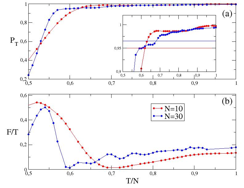
Figure 2: In panel (a) we plot target population as a function of the normalized operation time for different chain lengths ($N=10$ in red and $N=30$ in blue) obtained with OCT pulses. In panel (b) we observe the fluence of the OCT pulses as a function of the normalized operation time.

Now, we will assess the effect of disorder over the controlled transfer protocol. Fig. 3 shows how the static disorder, as described in the Sec. II, affects the target probability. The Figure also shows the free evolution for comparison. Fig. 3 show the averaged target probability $\langle P_{T}\rangle$, which is obtained from over $M=2000$ realizations of the disorder. For each realization of the disorder the target probability was obtained using the OCT protocol without disorder, and the averaged target probability is the unweighted average of all the realizations. The figure shows results for two different length chains ($N=10$ and $N=25$), choosing two values of $T_{OCT}$, namely $T_{OCT}\simeq T_{peak}$ and $T_{OCT}=N$, and the averaged target probability is plotted versus the disorder amplitude $A$. As expected with increasing values of $A$ the target probability decreases.

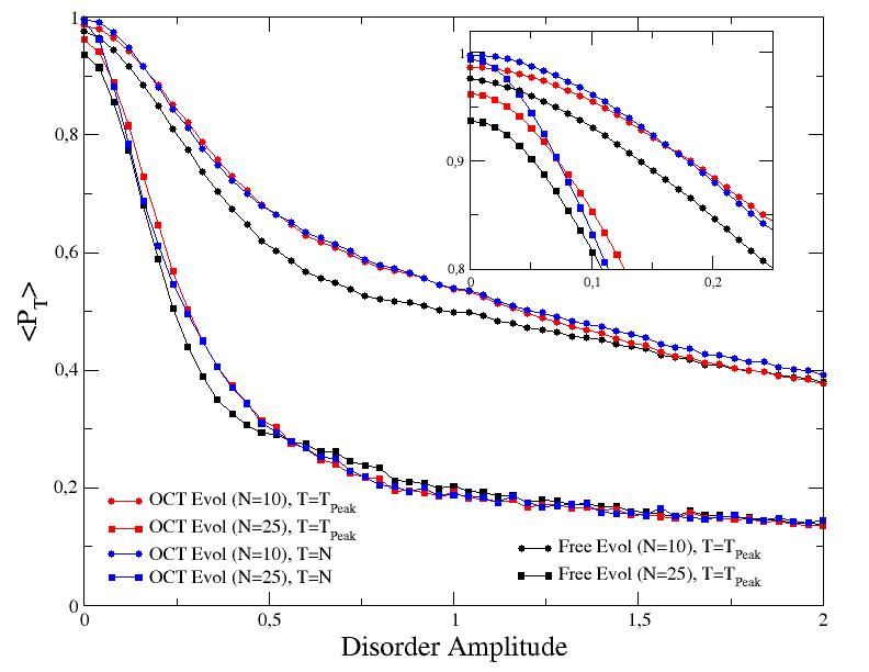
Figure 3: Target population averaged over $2000$ realizations as a function of Amplitude disorder for different chain lengths ($N=10$ with circles and $N=25$ with squares). In blue we observe target population for long pulses ($T_{OCT}=N$), in red for short pulses ($T_{OCT}=T_{peak}$) and in black we see the free evolution peak. The inset shows a zoom for small values of the amplitude disorder.

The inset in the figure shows that the better yield for very small disorder amplitude is obtained by using the optimized pulse for the larger operation time. However, a very small disorder amplitude destroys the improvement obtained by increasing the operation time. For amplitudes $A>0.1$ there is no difference between optimized evolution with $T_{OCT}=T_{peak}$ or $T_{OCT}=N$. This is not the case when we compare with the free evolution. We need to go to disorder amplitudes $A>1.5$ in order to obtain similar results using a free evolution strategy or employing an optimized pulse.

A simple way to improve the transmission using the free evolution strategy is to optimize the exchange coupling of the extremes $\alpha$ as was shown in several works Zwick1 ; Zwick2 ; Zwick3 . In Fig. 4 we plot the transfer probability for the free evolution at $T=T_{peak}$ as a function of $\alpha$. We also plot the target probability for the optimized dynamics for different operation times. All curves show a maximum close to $\alpha=0.6$. This result was known for the free evolution case. In this figure we observe an important advantage in the optimized evolution and the impaact of using large operation times. It is clear that, for $T_{OCT}=N$ we can use a wide range of $\alpha$ values, more than if we employ $T_{OCT}=T_{peak}$ and much more than in the free evolution case. It is worth to mention that, for the free evolution, exists a spurious shoulder related to peak times much larger than $N$ as we can observe in Fig. 4 (c).

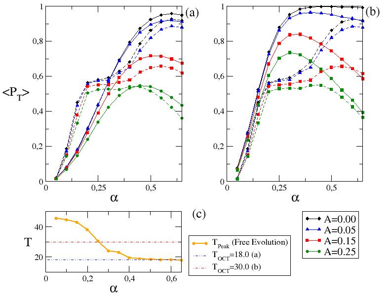
Figure 4: Upper panels show the averaged target population over $2000$ realizations as a function of the $N=30$ chain parameter $\alpha$ for OCT pulses (Continuous lines) and free evulotion (dasshed lines) for different disorder amplitudes. Panel (a) shows results for small operation time ($T_{OCT}=T_{peak}$ corresponding to the optimal $\alpha$, for $N=30$ we have $T\simeq 18$ a.u.) and panel (b) shows results for long operation time ($T_{OCT}=N$). Panel (c) shows $T_{peak}$ as a function of the $N=30$ chain parameter $\alpha$.

Finally, Fig. 5 shows the amplitude of the control pulse as a function of time, for different chain lengths. As can be observed, the pulses are appreciably different from zero in almost the same time interval for different values of $N$. This statement seems to be more accurate in the case of short pulses. In all the cases presented here, these times are shorter than the characteristic times where the free evolution lead to a maximum in the population transfer and shorter than the operation time in the OCT dynamics.

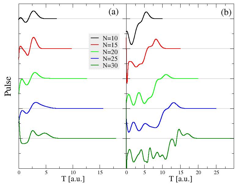
Figure 5: OCT pulses as a function of Time for different chain lengths. In (a) we plot short pulses ($T_{OCT}\simeq T_{peak}$) and in (b) we show the long pulses ($T_{OCT}=N$)

Interestingly, Figure 5 strongly suggest that the control pulses of shorter chains can be used as initial pulses for the OCT iterative procedure when dealing with larger chains. Moreover, it suggests that a simpler analytical pulse can be constructed in terms of the natural frequencies of the chain spectrum and some envelope function.

Optimal control theory, on the other hand, allows us to choose the desired time at which the maximum transfer is achieved, so synchronizing several signals to arrive at a given time is a certain possibility. Panel (b) of Fig. 5 shows what happens if longer arrival ($O(N)$) times are chosen. The pulses are, again, fairly simple but the number of frequencies involved increases with the transfer time, this behavior is consistent with the control pulses found in the literature that used control times on the order of $O(N^{2})$. In a sense, the high frequency pulses diminishes the net propagation speed of the excitation transfer process.

Here we want to return briefly to the results of Figure 1 to offer a qualitative description of how the transmission process is carried out with control pulses like those that we have calculated. In Fig. 1 (b) and (c) we can appreciate that the target population remains null while the pulse is appreciably different from zero. When the pulse dies and the evolution start to be a free evolution, the target population begins to rise. This can be understood as follows: the control pulse prepares a state that once it is prepared propagates along the spin chain until the population becomes localized at the other extreme of the chain. The pulse has an appreciable amplitude while the preparation takes place, but after this time there is no need for further driving. Besides, since the information propagates at the Quantum Speed Limit, the actuator can not affect the propagation once the state is “too far away”. Of course this semi-classical analysis should not be taken literally, but offers a good picture of the transfer process.

IV Control with two actuators

This Section is dedicated to analyze a different control strategy, using two actuators instead of just a single one, and assess if the physical traits found in the previous Section with respect to the control pulses, control time and robustness against static disorder are shared by more complex control strategies. To this end we implemented control equations where the first and last exchange couplings are time-dependent control functions. Despite the excellent controllability and the high population in the last site of the chain achieved after the transfer process, we want to explore here if the use of one more actuator enhances the good properties or if the trade off between simplicity and gains is not favorable.

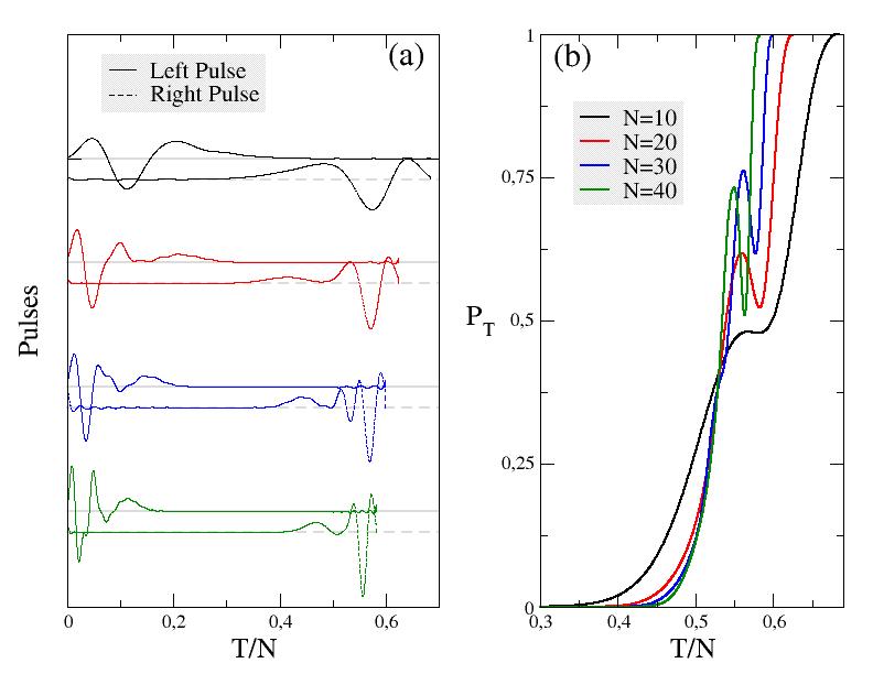
Figure 6: OCT dynamics with Two Actuators. (a) Pulses for different chain length as a function of the normalized time $T/N$. (b) Population of the target state as a function of the normalized time obtained with the OCT pulses showed in panel (b).

Figure 6 a) shows the control functions, as functions of the normalized time $T/N$, at both extremes of the chain and, from top to bottom, for chain lengths $N=10,20,30$ and $40$. The solid lines correspond to the control functions at the first exchange coupling and the dashed ones to the control functions at the last one. Both pulses, for a given chain length, were obtained as independent functions. Despite this, the reflection symmetry around one half of the normalized time is obvious. This result can be understood in terms of the reflection symmetry obeyed by the spin couplings that is characteristic of perfect state transfer schemes. This could be a practical recipe to look for control pulses with two actuators, i.e. instead of looking for two independent control pulses it could be more simpler to look for “reflected pulses” to be applied at the opposed ends of the chain. At any rate, the results presented in what follows were obtained assuming that the two control pulses were independent. It is worth to point that, again, the pulses for different chain lengths are closely related and that the pulses of shorter chains can be used as the initial pulses of the OCT method to find the optimized pulses of longer chains.

Figure 6 (b) shows the population at the last site of the chain obtained when the pulses shown in panel (a) control the dynamical behavior of the spin chain. The bigger difference with the rather monotonous behavior shown by the population growth when only one actuator is controlling the dynamics is the “shoulder” near $0.5T/N$ (see Figure 6).

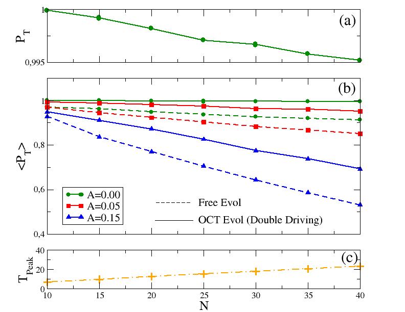
Figure 7: Disorder effect in the OCT evolution using two actuators. In panel (a) we show the yield as a function of the length chain for short OCT pulses using two actuators. The operation time employed in the transfer process $T_{OCT}=T_{peak}$ corresponding to he free evolution peak for the optimal $\alpha$ plotted in panel (c). In panel (b) we observe the effect of the disorder in the control operation

The robustness against static disorder for the two actuator case was analyzed in a similar way that the one actuator case. Using the control pulses designed to maximize the population transfer in an ordered chain we studied the population transfer in chains with static disorder. So, the results shown in Fig. 7 are averages over $M=2000$ realizations of the disorder. Panels (a), (b) and (c) of Fig. 7 show the maximum population transfer achieved, the averaged population at peak time for several disorder strengths, and the peak time, respectively, as functions of the chain length $N$. The data in Panel (c), show that the population transfer is achieved at peak times which change linearly when the chain length is increased. Panel (b) shows that, as expected, the controlled two-actuator scheme is far more robust against disorder than the free evolution of the border optimized chains, the population transfer corresponding to the two-actuators scheme (dots joines by solid lines) is always above the free evolution data (dots joined by dashed lines) and the decaying rate with the chain length is smaller. On the other hand, as shown in panel (a) the population transfer for the undisturbed chain is above $0.995$ even for $N=40$, which is excellent. It is important to remark that this level of control is achieved with low fluence pulses.

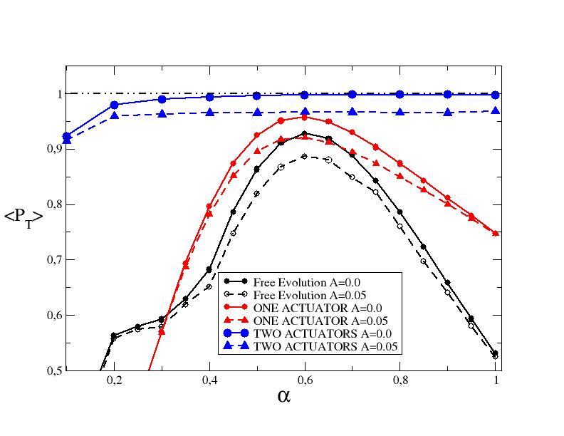
Figure 8: Averaged target population over $2000$ realizations as a function of the $N=30$ chain length $\alpha$ parameter for one actuator OCT pulses (red lines), for two actuators OCT pulses (blue lines) and for free evolution (black lines) with different disorder amplitudes. The result presented here are obtained for small operation time ($T_{OCT}=T_{peak}$ corresponding to the optimal $\alpha$, for $N=30$ we have $T_{OCT}\simeq 18$ a.u.)

The comparison between the one and two-actuators schemes performance is shown in Fig. 8. This figure shows the population transfer, with and without disorder, achieved with one and two-actuators schemes, for $N=30$. The free evolution is also depicted for comparison. The population transfer are shown, for all the cases, as functions of the border parameter $\alpha$. As shown by the Figure, the one actuator scheme and the free evolution depend strongly on this parameter, showing that it must be precisely tuned to attain a high population transfer. In contradistinction, the two actuator scheme is almost independent from it. As can be observed the two-actuator control achieves better population transfer than the one-actuator, even when the former is applied to disordered chains ($A=0.05$) and the later is applied to chains without disorder, except for a small interval of values of $\alpha$ near $\alpha=0$. This observation shows that the two-actuator scheme clearly outperforms the one-actuator one, of course barring any difficulties associated to the fact that the population transferred must be checked in one of the spins over which one of the actuators is acting.

V Conclusions

The results presented in the previous Sections show that, using OCT, it is possible to design smooth, simple and reliable control pulses, that transfer population from one extreme of a $XX$ spin chain to the other. The transfer can be achieved choosing the arrival time, as long as this time is longer or similar to the time compatible with the QSL, $T_{QSL}\approx N/2$. Moreover, in the one-actuator scheme, if the arrival time is chosen similar to $T_{QSL}$ the pulses will have very good properties as low fluence and the switch-off can be made smoothly and without a precise time control since the last part of the pulse has a very small amplitude and hardly affects the population transfer.

In the case of the two-actuator scheme, even for moderate chain lengths, the pulses act in (practically) different time intervals so, despite that an actuator has been added, there is no need of a precise timing between the two pulses. If this were not the case probably the need of a highly precise timing between the pulses could spoil the higher population transfer gained using two actuators instead of just one. If a two-actuator strategy were not feasible, tuning the value of the last exchange coupling constant contributes effectively to increase the population transfer.

It is necessary to remark the incredible robustness against the $\alpha$ parameter change of the two actuator protocol. For small operation times the difference with the one actuator protocol is huge. As we observe in Fig. 8 the one actuator protocol and the free evolution have a maximum for $\alpha\simeq 0.6$ while the double driving protcol shows an almost constant behaviour with values of the yield higher in all the range of the $\alpha$ parameter showed here. In the case of long operation times the differences between both protocols is not so important for values of $\alpha\geq 0.3$ as shown in Fig. 8 and Fig. 4.

Most studies that can be found in the literature consider that the control is exerted by external magnetic fields, which is natural for Magnetic Nuclear Resonance scenarios in liquids. For solid state settings, as quantum dots or superconducting qubits chains, the manipulation of the couplings between adjacent sites seems more achievable and faster.

Our findings also support the conclusion that systems with a QSL for the propagation of information should be controllable at times compatibles with such limit, in this sense we are working with other quantum spin chains to verify this. In particular we are interested if this limit can be achieved controlling exchange couplings or magnetic fields within schemes with at most two actuators acting over fixed sites.

Acknowledgments A. F., and S. S. G. acknowledge financial support from CONICET (PIP11220150100327, PUE22920170100089CO). O.O. acknowledges partial financial support from CONICET and SECYT-UNC. A.F. thanks the warm hospitality of the FAMAF, National University of Córdoba where this collaboration initiated.

References

- (1) S. Bose, Phys. Rev. Lett. 91, 207901 (2003).
- (2) G.M. Nikolopoulos and I. Jex (Edts.), Quantum State Transfer and Network Engineering, Springer-Verlag Berlin Heidelberg 2014
- (3) S. Bose, Contemporary Physics, 48:1, 13-30 (2007)
- (4) V. Kostak, G. M. Nikolopoulos, and I. Jex, Phys. Rev. A 75, 042319 (2007)
- (5) D. M. Zajac, T. M. Hazard, X. Mi, E. Nielsen, and J. R. Petta, Phys. Rev. Applied 6, 054013 (2016).
- (6) X. Li, Y. Ma, J. Han, Tao Chen, Y. Xu, W. Cai, H. Wang, Y.P. Song, Zheng-Yuan Xue, Zhang-qi Yin, and Luyan Sun, Phys. Rev. Applied 10, 054009 (2018)
- (7) Jingfu Zhang, Gui Lu Long, Wei Zhang, Zhiwei Deng, Wenzhang Liu, and Zhiheng Lu, Phys. Rev. A 72, 012331 (2005); P. Cappellaro, C. Ramanathan, and D. G. Cory, Phys. Rev. A 76, 032317 (2007); J. Zhang, M. Ditty, D. Burgarth, C. A. Ryan, C. M. Chandrashekar, M. Laforest, O. Moussa, J. Baugh, and R. Laflamme, Phys. Rev. A 80, 012316 (2009)
- (8) N. J. S. Loft et al New J. Phys. 18 045011 (2016).
- (9) L. Banchi, A. Bayat, P. Verrucchi, and S. Bose, Phys. Rev. Lett. 106, 140501 (2011).
- (10) R. J. Chapman, M. Santandrea, Zixin Huang, G. Corrielli, A. Crespi, Man-Hong Yung, R. Osellame and A. Peruzzo, Nat. Comm. 7, 11339 (2016).
- (11) Chang-Yu Hsieh, Yun-Pil Shim, M. Korkusinski and P. Hawrylak, Rep. Prog. Phys. 75, 114501 (2012).
- (12) D.S.A. Coden, S.S. Gomez, R.H. Romero, O. Osenda and A. Ferrón, Physica Scripta 94 (2), 025101 (2019).
- (13) M. Christandl, N. Datta, A. Ekert, and A. J. Landahl, Phys. Rev. Lett. 92,187902 (2004).
- (14) M. Christandl, N. Datta, T. C. Dorlas, A. Ekert, A. Kay, and A. J. Landahl, Phys. Rev. A 71, 032312 (2005).
- (15) Man-Hong Yung, Phys. Rev. A 74, 030303(R) (2006).
- (16) D. Burgarth and S. Bose, Phys. Rev. A 71, 052315 (2005).
- (17) D. Burgarth and S. Bose, New Journal of Physics 7, 135 (2005).
- (18) A. Zwick and O. Osenda, J. Phys. A: Math. Theor. 44 105302 (2011).
- (19) A. Zwick, G. A. Álvarez, J. Stolze, and O. Osenda, Phys. Rev. A 84, 022311 (2011).
- (20) A. Zwick, G. A. Álvarez, J. Stolze and O. Osenda, Quantum Information and Computation 15, 0582 (2015).
- (21) L. Banchi, T. J. G. Apollaro, A. Cuccoli, R. Vaia, and P. Verrucchi, Phys. Rev. A 8̱2, 052321 (2010).
- (22) L. Banchi, T. J. G. Apollaro, A. Cuccoli, R. Vaia and P. Verrucchi, New J. Phys. 13, 123006 (2011).
- (23) V. Jurdjevic and H. J. Sussmann, J. Diff. Eqn. 12, 313 (1972).
- (24) V. Ramakrishna, M. V. Salapaka, M. Dahleh, H. Rabitz, and A. Peirce, Phys. Rev. A 51, 960 (1995).
- (25) D. Burgarth, S. Bose, C. Bruder, and V. Giovannetti, Phys. Rev. A 79, 060305(R) (2009).
- (26) X. Wang, D. Burgarth, and S. Schirmer, Phys. Rev. A 94, 052319 (2016).
- (27) D. Burgarth, K. Maruyama, M. Murphy, S. Montangero, T. Calarco, F. Nori, and M. Plenio, Phys. Rev. A 81, 040303(R) (2010).
- (28) D. Stefanatos and E. Paspalakis, Phys. Rev. A 99, 022327 (2019).
- (29) G. Watanabe, Phys. Rev. A A 81, 021604(R) (2010).
- (30) S. Baumann, W. Paul, T. Choi, C. P. Lutz, A. Ardavan, and A. J. Heinrich, Science 350, 417 (2015).
- (31) K. Yang, Y. Bae, W. Paul, F. D. Natterer, P. Willke, J. L. Lado, A. Ferrón, T. Choi, J. Fernández-Rossier, A. J. Heinrich, and C. P. Lutz, Phys. rev. lett. 119, 227206 (2017).
- (32) Y. Bae, K. Yang, P. Willke, T. Choi, A. J. Heinrich, and C. P. Lutz, Science advances 4, eaau4159 (2018).
- (33) B. Bryant, R. Toskovic, A. Ferrón, J. L. Lado, A. Spinelli, J. Fernández-Rossier, and A. F. Otte, Nano Lett. 15, 6542 (2015).
- (34) A. Spinelli, B. Bryant, F. Delgado, J. Fernández-Rossier, and A. F. Otte, Nat. Mater. 13, 782 (2014).
- (35) J. Gong and P. Brumer, Phys. Rev. A 75, 032331 (2007).
- (36) P. M. Poggi and D. A. Wisniacki, Phys. Rev. A 94, 033406 (2016).
- (37) M. Murphy, S. Montangero, V. Giovannetti, T. Calarco, Phys. Rev. A 82, 022318 (2010).
- (38) D. Petrosyan, G. M. Nikolopoulos, and P. Lambropoulos, Phys. Rev. A 81, 042307 (2010).
- (39) X. Wang, A. Bayat, S. G. Schirmer, and S. Bose, Phys. Rev. A 81, 032312 (2010).
- (40) R. Heule, C. Bruder, D. Burgarth, and V. M. Stojanovic, Phys. Rev. A 82, 052333 (2010).
- (41) Werschnik, J and Gross, EKU, Journal of Physics B: Atomic, Molecular and Optical Physic, 40, R175 (2007).
- (42) Kosloff, Ronnie and Rice, Stuart A and Gaspard, Pier and Tersigni, Sam and Tannor, DJ, Chemical Physics 139, 201 (1989)
- (43) Putaja, A and Räsänen, E, Phys. Rev. B 82, 165336 (2010)