Unsupervised Cross-Domain Speech-to-Speech Conversion with Time-Frequency Consistency

Abstract

In recent years generative adversarial network (GAN) based models have been successfully applied for unsupervised speech-to-speech conversion. The rich compact harmonic view of the magnitude spectrogram is considered a suitable choice for training these models with audio data. To reconstruct the speech signal first a magnitude spectrogram is generated by the neural network, which is then utilized by methods like the Griffin-Lim algorithm to reconstruct a phase spectrogram. This procedure bears the problem that the generated magnitude spectrogram may not be consistent, which is required for finding a phase such that the full spectrogram has a natural-sounding speech waveform. In this work, we approach this problem by proposing a condition encouraging spectrogram consistency during the adversarial training procedure. We demonstrate our approach on the task of translating the voice of a male speaker to that of a female speaker, and vice versa. Our experimental results on the Librispeech corpus show that the model trained with the TF consistency provides a perceptually better quality of speech-to-speech conversion.

Index Terms: voice conversion, generative models,generative adversarial networks, time frequency consistency

1 Introduction

Deep generative models (GMs) form probabilistic models of the data generating distribution. In recent years GMs have attracted a lot of interest due to advancement in deep learning methods and computational resources which allowed for breakthroughs in various areas of application. An especially promising class of models are generative adversarial networks (GANs) [1], which build on an adversarial training setup to efficiently generate samples from high dimensional probability distributions. The application of GAN-based models led to state-of-the-art performance for various computer vision tasks, e.g. the generation of high-resolution images [2, 3, 4] and image-to-image translation [5, 6]. More recently, GANs have also been employed to speech-to-speech conversion [7, 8]. Systems for speech-to-speech conversion are of practical interest since they e.g. can be used to prevent privacy by voice morphing in online gaming platforms, or to artificially increase data sets for training neural network (NN) based speech recognition systems.

In recent GMs for speech-to-speech conversion [9, 10, 11] a WaveNet [12] like vocoder is used to generate the speech in an autoregressive step-wise manner. This comes at the cost of slow inference making these approaches impractical for real time applications. In contrast, using the time-frequency (TF) representation allows for parallel generation of the entire waveform which makes the inference much faster. Therefore, many recently proposed GAN based speech-to-speech conversion systems utilize the TF representation [7, 8, 13]. This, however, gives rise to another challenge: the TF representation consists of two parts, the magnitude and the phase spectrogram, and the noisy nature of the phase spectrogram makes it difficult for NNs to extract meaningful information. For this reason many NN based approaches only make use of the magnitude part and employ methods like the Griffin-Lim algorithm (GLA) [14] for reconstructing the time-domain waveform. This generally introduces artifacts and results in a low speech quality if the magnitude spectrogram is not consistent, i.e. if it can not be obtained by taking a short time Fourier transform (STFT) of any time-domain waveform.

Recently, it was shown that TF representations can improve audio generation by monitoring the consistency of generated magnitude spectograms based on a newly proposed consistency measure [15]. Inspired by this measure, we propose a consistency term to augment an adversarial training objective for unsupervised speech-to-speech conversion. More specifically, our main contributions are the following: (i) we implement a GAN-based speech-to-speech system building on the prominent UNsupervised Image-to-image Translation (UNIT) architecture [6], which, to our knowledge, has not been employed for cross-domain speech-to-speech conversion before; (ii) we propose to augment the training objective by a spectrogram consistency constraint which fosters a coherent time-domain waveform reconstruction; (iii) we perform an experimental analysis demonstrating that the proposed consistency term leads to a faster convergence of the iterative GLA and provides quantitative as well as qualitative improvements of the sample quality.

2 Related Work

In the last few years different NN based approaches utilizing a TF representation for speech-to-speech conversion have been proposed. The authors of [7] proposed a cycleGAN [5] network for cross-domain adaptation of speech signals utilising the magnitude spectrogram and making use of multiple discriminators on different frequency bands to allow the generator to focus on fine-grained features. The cycleGAN framework has also been employed for converting the voice of one speaker to another [8]. In [13] the authors proposed a variational autoencoder (VAE) [16] based architecture for voice conversion that jointly uses two types of spectral features. Another recent work [17] proposes an autoencoder framework for zero-shot voice conversion. The main problem of working with a TF representation for generation is in handling the irregularities present in the phase spectrogram. For this reason, an empirical measure of the TF consistency for monitoring the adversarial generation of magnitude spectrogram was proposed in [15]. Recently, [18] proposed GANsynth, a GM for music which avoids the phase reconstruction by proposing a model that builds on the full TF representation and uses the inverse-STFT (ISTFT) operations to get the time-domain waveform. To be able to do so, the noisy phase spectra is transformed into an instantaneous frequency representation.

In contrast to the existing work our focus lies on improving the consistency of the TF representation for the task of speech-to-speech conversion. Unlike [15] where consistency is used for monitoring the training, we propose to use it for an adversarial training of our speech-to-speech framework. We base our analysis on the UNIT architecture which learns a shared latent space for samples across two domains and was shown to perform better than cycleGAN for image-to-image translation [6].

3 TF-consistent unsupervised speech-to-speech conversion

Our speech-to-speech conversion network is based on the UNIT architecture introduced for image-to-image translation in [6]. In this section we first give a brief description of the UNIT framework and TF consistency. We then introduce the TF constraint for speech-to-speech conversion.

3.1 The UNIT framework

Let $\mathcal{X}_{1}$ and $\mathcal{X}_{2}$ be two domains (e.g. representing speech of male and female speakers) and $\mathcal{Z}$ be a shared latent space. Let us assume that for any pair $(x_{1},x_{2})$ of corresponding samples there exists a $z\in\mathcal{Z}$, which serves as a latent representation of $x_{1}$ and $x_{2}$ simultaneously. More specifically, we assume that there exist encoder functions $E_{1}$ and $E_{2}$ and decoder functions $G_{1}$ and $G_{2}$ such that, for a pair of corresponding samples $(x_{1},x_{2})$ and some $z\in\mathcal{Z}$, we have $E_{1}(x_{1})=E_{2}(x_{2})=z$ and $x_{1}=G_{1}(z)$, $x_{2}=G_{2}(z)$. For any $x_{1}\in\mathcal{X}_{1}$ or $x_{2}\in\mathcal{X}_{2}$ we can then obtain the corresponding cross domain translation by the compositional mapping $G_{2}(E_{1}(x_{1}))$ or $G_{1}(E_{2}(x_{2}))$, respectively. The shared latent space is implemented using cycle consistency loss and parameter sharing between the last layer of $E_{1}$ and $E_{2}$ and between the first layer of $G_{1}$ and $G_{2}$.

In the UNIT architecture the pairs $\{E_{1},G_{1}\}$ and $\{E_{2},G_{2}\}$ constitute VAEs. Moreover, the framework contains two discriminators $D_{1}$ and $D_{2}$, and $\{G_{1},D_{1}\}$ and $\{G_{2},D_{2}\}$ form GANs. The objective function consists of various loss terms. The VAE loss for domain $\mathcal{X}_{i},i\in\{1,2\}$, is defined as $L_{\text{VAE}}(E_{i},G_{i})=$

$$\lambda_{1}KL(q_{i}(z_{i}|x_{i})||p(z))+\lambda_{2}\mathbb{E}_{z_{i}\sim q_{i}(z_{i}|x_{i})}[\log p_{G_{i}}(x_{i}|z_{i})]$$ (1)

where $q_{i}(z_{i}|x_{i})=\mathcal{N}(z_{i}|E_{i}(x_{i}),I)$, $p(z)=\mathcal{N}(z|0,I)$, $p_{G_{i}}$ is a Laplacian distribution and $KL$ is the Kullback-Leibler divergence. The cycle consistency loss for the translation cycle $\mathcal{X}_{i}\rightarrow\mathcal{X}_{j}\rightarrow\mathcal{X}_{i}$ is defined as $L_{CC}(E_{i},G_{i},E_{j},G_{j})=$

$$\lambda_{3}(KL(q_{i}(z_{i}|x_{i})||p_{\eta}(z))+KL(q_{j}(z_{j}|x_{i}^{i\rightarrow j})||p_{\eta}(z)))$$

$$+\lambda_{4}\mathbb{E}_{z_{j}\sim q_{j}(z_{j}|x_{i}^{i\rightarrow j})}[\log p_{G_{i}}(x_{i}|z_{j})]$$ (2)

In contrast to UNIT we use the LS-GAN objective [19] to avoid the vanishing gradient problem and to ensure a stable training. The adversarial LS-GAN loss $L_{\text{GAN}}(E_{j},G_{i},D_{i})$ for domain $\mathcal{X}_{i}$ is defined as:

$$\frac{1}{2}\cdot(\mathbb{E}_{x_{i}\sim p_{\mathcal{X}_{i}}}[(\mathcal{D}_{i}(x_{i})^{2}]+\mathbb{E}_{z_{j}\sim q_{j}(z_{j}|x_{j})}[(1-\mathcal{D}_{i}(\mathcal{G}_{i}(z_{j})))^{2}])$$ (3)

The full training objective combines the loss functions for both VAEs with GAN and cycle-consistency loss. The full objective is given as:

$$\min_{E_{1},G_{1},E_{2},G_{2}}\max_{D_{1},D_{2}}L_{\text{VAE}}(E_{1},G_{1})+L_{\text{GAN}}(E_{2},G_{1},D_{1})$$

$$\qquad\qquad+L_{\text{VAE}}(E_{2},G_{2})+L_{\text{GAN}}(E_{1},G_{2},D_{2})$$

$$+L_{CC}(E_{1},G_{1},E_{2},G_{2})+L_{CC}(E_{2},G_{2},E_{1},G_{1})$$ (4)

The encoder functions are implemented as NNs consisting of three convolution layers, followed by four ResNet blocks [20]. Likewise the decoders are given by NNs with four ResNet blocks of the same configuration followed by three upsampling blocks with an upsampling factor of $2$. For further details we refer to the original publication [6].

3.2 TF Consistency

The GLA is a well known technique for estimating the closest waveform from a given magnitude spectrogram. It estimates the unknown phase by iteratively performing ISTFT and STFT operation to project the spectrogram between the time and frequency domain and thus minimizing the projection error. A critical requirement for convergence is the consistency of the spectrogram representation, that is if there exists a valid time-domain waveform associated with the spectrogram. Formally, a spectrogram $W\in\mathbb{C}^{M\times N}$ is consistent if it is an element of the null space of the linear transformation $\text{STFT}(\text{ISTFT}(W))-W$. An alternative necessary condition for the consistency of any log magnitude matrix $\log(M_{g}(x,\omega))$ for a Gaussian window with variance $\lambda$ under the STFT operation was given in [21] as:

$$\left(\lambda\frac{\partial^{2}}{\partial x^{2}}+\lambda^{-1}\frac{\partial^{2}}{\partial\omega^{2}}\right)\log(M_{g}(x,\omega))=-2\pi\enspace.$$ (5)

This equation resembles the condition of analytic functions where the Laplacian of the log magnitude spectrogram $\log(M_{g}(x,\omega))$ is constant. Thus, the consistency of the spectrogram could be interpreted as finding a solution in the analytic space of spectrograms. For further details we recommend [21].

By replacing the derivatives with finite differences the (5) can be approximated as

$$\left(\frac{\lambda}{a^{2}}{\partial_{n}^{2}}+K^{2}\lambda^{-1}{\partial_{m}^{2}}\right)\log(M_{g}[m,n])\approx-2\pi$$ (6)

where $a$ is the stride length, $K$ is the number of frequency bins, $n$ is the time step, $m$ is the frequency step in the STFT matrix, $\partial_{n}^{2}$, $\partial_{m}^{2}$ are second order derivative along time and frequency step. In [15] the (6) is utilized to derive a consistency measure which leads to improved sample quality when used to monitor the training of a GAN. They define an empirical consistency measure $\rho$ for a generated magnitude spectrogram $M$ as $\rho(M)=r(\text{DM}_{n},\text{DM}_{m})$ with

$$\text{DM}_{n}=\left\lvert\partial_{n}^{2}M+\frac{\pi a^{2}}{\lambda}\right\rvert\;\;\text{and}\;\;\text{DM}_{m}=\left\lvert\partial_{m}^{2}M+\frac{\pi\lambda}{K^{2}}\right\rvert,$$ (7)

and $r(X,Y)$ being the sample Pearson correlation coefficient of a paired set of samples $(x,y)$. For a consistent spectrogram (6) holds, thus $\rho(M)\approx 1$ and for an inconsistent spectrogram $\rho(M)\approx 0$. Extending this idea to adversarial training the consistency term which is monitored along with the min-max-loss of GANs is defined as

$$\gamma=\left\lvert\mathbb{E}_{M_{r}\sim p_{M_{\text{real}}}}[\rho(M_{r})]-\mathbb{E}_{M_{f}\sim p_{M_{\text{fake}}}}[\rho(M_{f})]\right\rvert\enspace,$$ (8)

where $p_{M_{\text{real}}}$ represents the probability distribution of real spectrograms and $p_{M_{\text{fake}}}$ represents the probability distribution of fake spectrograms. As $\gamma\rightarrow 0$ the consistency term $\rho(M_{f})\rightarrow 1$. For further details, we refer the interested reader to [15].

3.3 TF consistent speech-to-speech conversion

Following the above formulation, we define the spectrogram consistency loss in our speech-to-speech synthesis framework. For a source spectrogram $x_{1}\in\mathcal{X}_{1}$ we define the consistency of the corresponding cross-domain spectrogram $x_{2}=G_{2}(E_{1}(x_{1}))$ as $\gamma_{x_{2}}$. Conversely, we also define $\gamma_{x_{1}}$ and the final consistency term is given by $\gamma$ as $\gamma=\gamma_{x_{1}}+\gamma_{x_{2}}$ with

$$\begin{split}\gamma_{x_{2}}=\left\lvert\mathbb{E}_{x_{2}\sim p_{\mathcal{X}_{2}}}[\rho(x_{2})]-\mathbb{E}_{x_{1}\sim p_{\mathcal{X}_{1}}}[\rho(G_{2}(E_{1}(x_{1}))]\right\rvert,\end{split}$$ (9a)

$$\begin{split}\gamma_{x_{1}}=\left\lvert\mathbb{E}_{x_{1}\sim p_{\mathcal{X}_{1}}}[\rho(x_{1})]-\mathbb{E}_{x_{2}\sim p_{\mathcal{X}_{2}}}[\rho(G_{1}(E_{2}(x_{2}))]\right\rvert\end{split}$$ (9b)

Due to adversarial critic form of $\gamma$, we utilize it in the training of UNIT framework by adding $\lambda_{c}\cdot\gamma$ as an additional term in the objective function stated in (3.1), where $\lambda_{c}$ is a hyperparameter to control the contribution of the consistency loss. We will later see that adding $\lambda_{c}\cdot\gamma$ to the training loss results in a perceptual improvement for our voice conversion task.

4 Experiments

4.1 Dataset and Preprocessing

We use the LibriSpeech corpora [22] for our experiments which is a dataset obtained from English audiobooks read by native English speakers. Table 1 describes the statistics of the dataset. We used the provided training set (train-clean-100) for training and the provided test set (test-clean-100) for evaluation.

Table 1: Data Statistics of LibriSpeech Corpus

	Train	Test
Sampling Rate	16 kHz	16 kHz
Total Duration	100.6 hrs.	5.4 hrs
Per Spk. Duration	25 min.	8 min.
Female Speakers	125	20
Male Speakers	126	20

The speech files in the LibriSpeech are of varying length. To train our network we work with a fixed-length representation, i.e. we split each speech file into segments of $4$ seconds. This way, we end up with $48,301$ samples of female and $48,139$ samples of male speech. To obtain the TF representation, we use the STFT transformation with $512$ frame size, Hanning window, $128$ hop length, and $75$% overlap. As speech signals are real-valued signals, we trim the representation at the Nyquist frequency. Finally, we obtain a matrix of size $500\times 256$, where $500$ is the number of time steps and $256$ is the frequency bin. To ensure that the samples have the same loudness range and that the representation matches the range of the tanh activation functions of the generators output neurons, we re-scale all coefficients in the matrix to lie in the range $[-1,1]$.

4.2 Network details and training setup

We aim to investigate the effect of encouraging TF consistency in GAN-based cross domain speech-to-speech conversion. We use the vanilla UNIT network as our baseline model, since it was reported to lead to results superior to those of the cycleGAN for unsupervised image to image translation [6]. To indicate that it is applied to speech instead of image translation, we refer to this baseline model as UNST and call the model trained with our consistency term (9) proposed in Section 3.2 as C-UNST.

We trained all models for 1,000,000 iterations with the Adam optimizer [23] with an initial learning rate of $0.0001$ (which was decayed by a factor of $0.5$ every 100,000 iterations), the momentum parameters $\beta_{1}=0.5$ and $\beta_{2}=0.999$, and weight decay with a hyperparameter of $0.0001$. Due to the high computational cost, we avoid extensive hyperparameter tuning. We set the weights of the loss terms presented in (1) and  (3.1) to $\lambda_{1}=\lambda_{3}=0.01$, $\lambda_{2}=\lambda_{4}=10$. We initialize the tuning parameter of the spectrogram consistency term $\lambda_{c}$ with a value of $3e^{-4}$ and decayed it by a factor of $0.9$ every $10,000$ iterations, which resulted in all weighted loss terms being of similar scale. Our implementation was done using NNabla, a NN framework developed by Sony and our experiments were executed on GeForce GTX 1080 Ti GPU with $11$ GB of memory.

4.3 Evaluation

We perform a quantitative as well as qualitative evaluation of the generated speech samples. We report all measures on the test set.

For quantitative evaluation, we compare the statistics of real and generated data using the Frećhet inception distance (FID) [24]. The FID requires a feature representation of the spectrogram. Therefore, we trained the time-delay NN used in [25] on the speaker identification task using LibriSpeech train set. We used 70% samples for training and 30% for evaluation for which we obtained an accuracy of $0.875$. We use it as a feature extractor. Moreover, we trained a classifier to discriminate between the voice of male and female speakers, to access the quality of the translation. We implement it as a fully connected NN with $2$ hidden layers, with $512$ and $256$ units respectively, and LeakyReLU [26] with a slope of $0.2$.We used the train set of LibriSpeech for training and got an accuracy of $0.975$ on the test set of $40$ speakers, which serves as the benchmark accuracy of domain classification.

For qualitative evaluation, we conduct two perceptual evaluation tests with 28 participants. In the first test, we ask listeners to rate the quality of translated speech samples on a scale: Excellent (80-100), Good (60-80), Fair (40-60), Poor (20-40) and Bad (0-20). In the second test, we ask listeners to rate the extent to which each translated sample sound like a female or male person. For this we use a scale: Female (80-100), Somewhat Female (60-80), Not sure (40-60), Somewhat Male (60-80) and Male (80-100). In both tests, we arbitrarily selected $11$ samples of male and female speakers from the test set. We use webMUSHRA [27] to set up the online human evaluation test. We report the mean opinion score (MOS) for each model.

5 Results and Discussion

In this section we will present the results of the quantitative and qualitative evaluation, as well as of an ablation study.

5.1 FID based quantitative evaluation

Table 2 compares the performance of UNST and C-UNST on male to female (M2F) and female to male (F2M) conversion for magnitude and log magnitude spectrograms. The results show that the log transformation generally helps the training and leads to lower FID scores. The log transformation spreads the spectrogram by enhancing the lower components and compressing the noise part which makes it easier for the models to learn meaningful features. Moreover, the C-UNST clearly outperforms the UNST in terms of FID scores.

Table 2: Evaluation of generated samples on held out set of 40 speakers for evaluation.

Method	Spectrogram	FID		Accuracy
		F2M	M2F
UNST	Mag	130.32	100.36	0.894
	LogMag	$\mathbf{76.90}$	$\mathbf{74.18}$	$\mathbf{0.935}$
C-UNST	Mag	94.83	83.52	$\mathbf{0.928}$
	LogMag	$\mathbf{70.11}$	$\mathbf{69.50}$	0.860

5.2 Effect of different loss terms

The objective function we employ for training our model comprises several loss terms. To understand the effects of these different terms we perform an ablation study, where we removed different parts of the C-UNST objective. The effects on the FID scores are reported in Table 3. The results show that including the KL loss terms in (1) and (3.1) did not provide any improvement in terms of the FID. The removal of the KL terms reduces $\{E_{1},G_{1}\})$ and $\{E_{2},G_{2}\}$ to vanilla autoencoders, which seem to be sufficient for the framework. The cycle consistency term in (3.1) is useful for the magnitude representation but not for the log magnitude. We hypothesize this could be due to the weight sharing condition in UNIT which additionally ensures that a pair of corresponding samples from the two domains are represented by the same latent features. To validate this we removed the cycle consistency loss, as well as the weight sharing. In this case, we observed that the model performs poorly at the task of voice conversion.

Table 3: Effect of different loss terms on FID scores top M2F and bottom F2M. The C-UNST is our proposed model, UNST is obtained by setting $\lambda_{c}=0$, No KL is obtained by setting $\lambda_{c}=\lambda_{1}=\lambda_{3}=0$, No CC is obtained by setting $\lambda_{c}=\lambda_{1}=\lambda_{3}=\lambda_{4}=0$ and No Shared-CC is obtained by setting $\lambda_{c}=\lambda_{1}=\lambda_{3}=\lambda_{4}=0$ and removing parameter sharing between last layer of $E_{1}$ and $E_{2}$ and first layer of $G_{1}$ and $G_{2}$.

Spectrogram	C-UNST	UNST	No KL	No CC	No Shared-CC
			M2F
Mag	94.83	130.32	87.08	2491.03	408.45
LogMag	70.11	76.90	74.88	94.71	420.11

Spectrogram	C-UNST	UNST	No KL	No CC	No Shared-CC
			F2M
Mag	83.52	100.36	81.57	1273.12	4209.07
LogMag	69.50	74.18	69.14	108.09	730.16

Finally, Figure 1 gives a pair of examples of a spectograms for two test samples and corresponding translation using C-UNST.

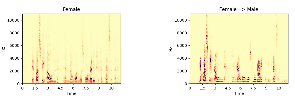
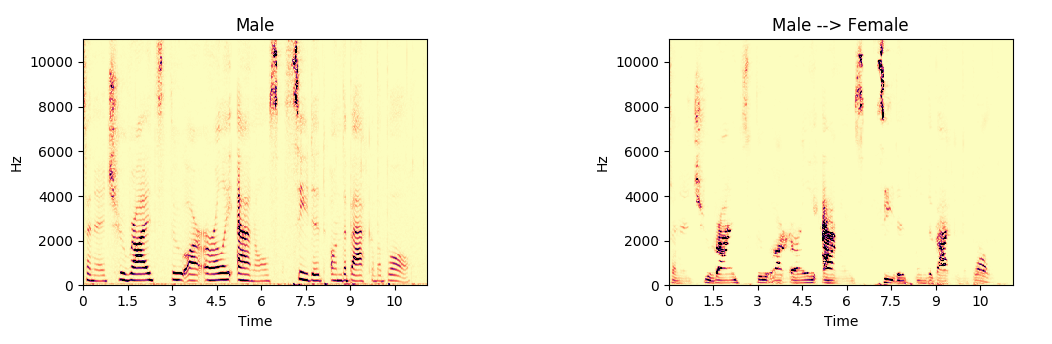
Figure 1: Examples of a spectrograms of four second segments for the data set and the corresponding translation generated by a C-UNST. The model learned to shift the pitch contour as well as to change the spectral envelope to translate the voice.

Table 4: Mean opinion scores on the general quality of the generated sample and the degree of how much it belongs to the corresponding domain (male or female). Bold printed values indicate a statistical significance of the difference with a significance level smaller than $0.001$ according to pair-wise Wilcoxon signed-rank test [28]

Method	MOS
	Quality		Domain
	M2F	F2M	M2F	F2M
UNST	64.66	76.28	82.62	87.18
C-UNST	$\mathbf{70.13}$	$76.29$	$\mathbf{88.44}$	$\mathbf{89.50}$

5.3 MOS-based qualitative evaluation

We only consider models trained on the log magnitude spectrogram for the MOS evaluation, since they achieved better results in the quantitative evaluation. The results are given in Table 4. The C-UNST clearly outperforms the UNST in terms of the quality of the translated samples as well as in terms of how much the M2F translated samples sound female. The F2M translated samples were rated similarly for both models. These results are consistent with the FID scores, indicating overall that the TF consistency leads to a clear improvement of quantitative as well as qualitative sample quality.

6 Conclusions

We introduced an adversarial framework for unsupervised cross-domain speech-to-speech conversion. We utilized the consistency condition of the magnitude-spectrogram to constrain the learning such that translated spectrograms have a valid time-domain waveform. We demonstrated the performance of our model on the task of translating the voice of male to the voice of female speakers and vice versa and performed a quantitative as well as a qualitative evaluation. Our consistency based model achieved lower FID and better MOS scores.

References

- [1] I. Goodfellow, J. Pouget-Abadie, M. Mirza, B. Xu, D. Warde-Farley, S. Ozair, A. Courville, and Y. Bengio, “Generative adversarial nets,” in Advances in neural information processing systems, 2014, pp. 2672–2680.
- [2] T. Karras, T. Aila, S. Laine, and J. Lehtinen, “Progressive growing of gans for improved quality, stability, and variation,” arXiv preprint arXiv:1710.10196, 2017.
- [3] C. Ledig, L. Theis, F. Huszár, J. Caballero, A. Cunningham, A. Acosta, A. Aitken, A. Tejani, J. Totz, Z. Wang et al., “Photo-realistic single image super-resolution using a generative adversarial network,” in Proceedings of the IEEE conference on computer vision and pattern recognition, 2017, pp. 4681–4690.
- [4] E. L. Denton, S. Chintala, R. Fergus et al., “Deep generative image models using a laplacian pyramid of adversarial networks,” in Advances in neural information processing systems, 2015, pp. 1486–1494.
- [5] J.-Y. Zhu, T. Park, P. Isola, and A. A. Efros, “Unpaired image-to-image translation using cycle-consistent adversarial networks,” in Proceedings of the IEEE international conference on computer vision, 2017, pp. 2223–2232.
- [6] M.-Y. Liu, T. Breuel, and J. Kautz, “Unsupervised image-to-image translation networks,” in Advances in Neural Information Processing Systems, 2017, pp. 700–708.
- [7] E. Hosseini-Asl, Y. Zhou, C. Xiong, and R. Socher, “A multi-discriminator cyclegan for unsupervised non-parallel speech domain adaptation,” Proc. Interspeech 2018, pp. 3758–3762, 2018.
- [8] T. Kaneko and H. Kameoka, “Parallel-data-free voice conversion using cycle-consistent adversarial networks,” arXiv preprint arXiv:1711.11293, 2017.
- [9] J. Niwa, T. Yoshimura, K. Hashimoto, K. Oura, Y. Nankaku, and K. Tokuda, “Statistical voice conversion based on wavenet,” in 2018 IEEE International Conference on Acoustics, Speech and Signal Processing (ICASSP). IEEE, 2018, pp. 5289–5293.
- [10] K. Kobayashi, T. Hayashi, A. Tamamori, and T. Toda, “Statistical voice conversion with wavenet-based waveform generation.” in Interspeech, 2017, pp. 1138–1142.
- [11] P. L. Tobing, Y.-C. Wu, T. Hayashi, K. Kobayashi, and T. Toda, “Voice conversion with cyclic recurrent neural network and fine-tuned wavenet vocoder,” in ICASSP 2019-2019 IEEE International Conference on Acoustics, Speech and Signal Processing (ICASSP). IEEE, 2019, pp. 6815–6819.
- [12] A. v. d. Oord, S. Dieleman, H. Zen, K. Simonyan, O. Vinyals, A. Graves, N. Kalchbrenner, A. Senior, and K. Kavukcuoglu, “Wavenet: A generative model for raw audio,” arXiv preprint arXiv:1609.03499, 2016.
- [13] W.-C. Huang, H.-T. Hwang, Y.-H. Peng, Y. Tsao, and H.-M. Wang, “Voice conversion based on cross-domain features using variational auto encoders,” in 2018 11th International Symposium on Chinese Spoken Language Processing (ISCSLP). IEEE, 2018, pp. 51–55.
- [14] D. Griffin and J. Lim, “Signal estimation from modified short-time fourier transform,” IEEE Transactions on Acoustics, Speech, and Signal Processing, vol. 32, no. 2, pp. 236–243, 1984.
- [15] A. Marafioti, N. Perraudin, N. Holighaus, and P. Majdak, “Adversarial generation of time-frequency features with application in audio synthesis,” in International Conference on Machine Learning, 2019, pp. 4352–4362.
- [16] D. P. Kingma and M. Welling, “Auto-encoding variational bayes,” arXiv preprint arXiv:1312.6114, 2013.
- [17] K. Qian, Y. Zhang, S. Chang, X. Yang, and M. Hasegawa-Johnson, “Autovc: Zero-shot voice style transfer with only autoencoder loss,” in International Conference on Machine Learning, 2019, pp. 5210–5219.
- [18] J. Engel, K. K. Agrawal, S. Chen, I. Gulrajani, C. Donahue, and A. Roberts, “Gansynth: Adversarial neural audio synthesis,” arXiv preprint arXiv:1902.08710, 2019.
- [19] X. Mao, Q. Li, H. Xie, R. Y. Lau, Z. Wang, and S. Paul Smolley, “Least squares generative adversarial networks,” in Proceedings of the IEEE International Conference on Computer Vision, 2017, pp. 2794–2802.
- [20] K. He, X. Zhang, S. Ren, and J. Sun, “Deep residual learning for image recognition,” in Proceedings of the IEEE conference on computer vision and pattern recognition, 2016, pp. 770–778.
- [21] F. Auger, É. Chassande-Mottin, and P. Flandrin, “On phase-magnitude relationships in the short-time fourier transform,” IEEE Signal Processing Letters, vol. 19, no. 5, pp. 267–270, 2012.
- [22] V. Panayotov, G. Chen, D. Povey, and S. Khudanpur, “Librispeech: an asr corpus based on public domain audio books,” in 2015 IEEE International Conference on Acoustics, Speech and Signal Processing (ICASSP). IEEE, 2015, pp. 5206–5210.
- [23] D. P. Kingma and J. B. Adam, “A method for stochastic optimization. iclr,” in 3rd International Conference on Learning Representations, 2014.
- [24] M. Heusel, H. Ramsauer, T. Unterthiner, B. Nessler, and S. Hochreiter, “Gans trained by a two time-scale update rule converge to a local nash equilibrium,” in Advances in Neural Information Processing Systems, 2017, pp. 6626–6637.
- [25] K. Okabe, T. Koshinaka, and K. Shinoda, “Attentive statistics pooling for deep speaker embedding,” Proc. Interspeech 2018, pp. 2252–2256, 2018.
- [26] A. L. Maas, A. Y. Hannun, and A. Y. Ng, “Rectifier nonlinearities improve neural network acoustic models,” in Proc. icml, vol. 30, no. 1, 2013, p. 3.
- [27] M. Schoeffler, S. Bartoschek, F.-R. Stöter, M. Roess, S. Westphal, B. Edler, and J. Herre, “webmushra—a comprehensive framework for web-based listening tests,” Journal of Open Research Software, vol. 6, no. 1, 2018.
- [28] F. Wilcoxon, S. Katti, and R. A. Wilcox, “Critical values and probability levels for the wilcoxon rank sum test and the wilcoxon signed rank test,” Selected tables in mathematical statistics, vol. 1, pp. 171–259, 1970.