The W. Thurston Algorithm
Applied to Real Polynomial Maps

Abstract

This note will describe an effective procedure for constructing critically finite real polynomial maps with specified combinatorics.

Keywords: Thurston algorithm, critically finite real polynomials, real critical points, piece-wise linear model, higher order critical points, local degree, framing points, expansiveness.

Mathematics Subject Classification (2020): 37F10, 37F20, 37E05, 37E25, 37M99.

1 Introduction.

The Thurston algorithm is a method for constructing critically finite rational maps with specified combinatorics. (Compare [DH].) In the general case, it requires quite a bit of work even to describe the algorithm precisely, much less to prove convergence; and the implementation is very difficult.

In this note we are concerned with the much easier case of real polynomial maps with real critical points. In this case, the result can be stated quite easily, and carried out without too much difficulty. (However the proof that the algorithm always converges in the polynomial case depends essentially on more difficult complex methods. We will simply refer to Bielefeld-Fisher-Hubbard [BFH] or Poirier [P1] for this.)

Section 2 will describe the data which must be presented to the algorithm in order for it to produce a corresponding uniquely defined critically finite real polynomial map. The hardest step in carrying out the algorithm, at least when the degree is four or more, is the construction of polynomials with prescribed critical values. Section 3 will use methods suggested by Douady and Sentenac to deal with this problem. Section 4 will then describe the actual algorithm. Appendix A deals with computational issues; Appendix B provides further examples, in particular for the non-expansive case; and Appendix C is a brief table providing more precise information about the various figures. The authors plan to publish a sequel about real quadratic rational maps (see [BMS] for a preliminary version).

Thurston’s presentation was based on iteration in the Teichmüller space for the Riemann sphere with finitely many marked points. Many people have contributed to or applied this theory or modifications of it. In addition to the papers cited above, see especially [Ba], [Ba-N], [HS], and [P2], as well as [H-He], [Ch] , and [J]. (The Hubbard-Schleicher paper starts with an explicit description of the Thurston algorithm for real quadratic polynomials.) For a completely different approach, see Dylan Thurston [T].

For access to our maple code, and for an interactive demonstration program, seehttps://www.math.stonybrook.edu/~scott/ThurstonMethod/

2 Combinatorics.

Let $f:{\mathbb{R}}\to{\mathbb{R}}$ be a real polynomial map of degree $d\geq 2$ which has real critical points $c_{1}\leq c_{2}\leq\cdots\leq c_{d-1}$. The derivative of $f$ can be written as

$$f^{\prime}(x)~{}=~{}a(x-c_{1})\cdots(x-c_{d-1})~{},\qquad{\rm with~{}leading~{}coefficient}\qquad a\neq 0~{}.$$

If we are given such an $f^{\prime}\!$, then of course $f$ is uniquely defined up to an additive constant. By definition, the real filled Julia set $K_{\mathbb{R}}(f)$ is the set of all real numbers $x$ for which the forward orbit of $x$ is bounded.

We will say that $f$ is in $\bm{K}_{\mathbb{R}}\!$-normal form if the smallest point of its real filled Julia set is $x=0$, and the largest one is $x=1$. This is very convenient for graphical purposes, since it means that all of the interesting dynamics of $f$ can be observed by looking at its graph restricted to the unit interval $I=[0,1]$, with all orbits outside of $I$ escaping to infinity. Evidently $f$ can be put into $K_{\mathbb{R}}$-normal form by a unique orientation preserving affine change of coordinates whenever $K_{\mathbb{R}}(f)$ contains at least two distinct points. (The exceptional cases where $K_{\mathbb{R}}(f)$ is empty, or consists of a single non-attracting fixed point are of no interest to us.)

For any map in $K_{\mathbb{R}}$-normal form, note that the boundary $\{0,\,1\}$ of $I$ necessarily maps into itself. There are four possible ways of mapping the boundary to itself, as illustrated in Figure 1.

Figure 1: For a map of odd degree in $K_{\mathbb{R}}$-normal form, the end points $0$ and $1$ are either fixed points or form a period two orbit according as the leading coefficient is positive or negative. On the other hand, for maps of even degree, both end points map to one of the two. The middle two graphs provide examples of maps for which $K_{\mathbb{R}}$ is not connected. In these examples, the critical points all lie in $[0,1]$ but the critical values do not.

Definition .

The map will be called critically finite if every critical orbit is periodic or eventually periodic. A map of degree $d$ has simple critical points if the $d-1$ critical points are all distinct. That is, putting the map in $K_{\mathbb{R}}\!$ normal form, they can be listed as

$$0<c_{1}<c_{2}<\cdots<c_{d-1}<1~{}.$$

(Later we will deal with higher order critical points, which may well be boundary points of the interval $[0,1]$. However, simple critical points are always interior points of the interval.) By the combinatorics of such a critically finite map with simple critical points we will mean the sequence of integers

$${\stackrel{{\scriptstyle\rightarrow}}{{m}}}~{}=~{}(m_{0},~{}m_{1},~{}\cdots~{},~{}m_{n})$$

constructed as follows. Let

$$0=x_{0}<x_{1}<\cdots<x_{n}=1$$

be the list consisting of all points which are either critical or postcritical, together with $0$ and $1$ (if they are not already included). Then there are unique integers $m_{0},\cdots,m_{n}$ between zero and $n$ such that $f(x_{j})=x_{m_{j}}$.

Our goal is to show that the map $f$ is uniquely determined and effectively computable from its combinatorics. More precisely, given a sequence $~{}{\stackrel{{\scriptstyle\rightarrow}}{{m}}}=(m_{0},\cdots,m_{n})$ satisfying a few simple necessary conditions, there is one and only one corresponding polynomial map in $K_{\mathbb{R}}$ normal form, and the coefficients of this polynomial can be explicitly computed.

There will be a corresponding statement for the more general case where critical points of higher multiplicity are allowed; and hence boundary critical points are also allowed. However we will stick to the simple case for the moment.

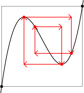
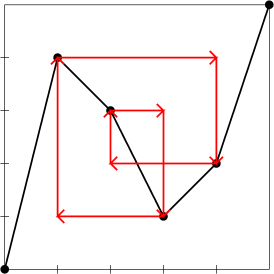
Figure 2: On the left, example of a cubic map $f$ with combinatorics $(0,4,3,1,2,5)$. Here the two critical points belong to a common period four orbit. The red arrows describe the dynamics. On the right, a corresponding graph for the piecewise-linear model of $f$, as described below. See LABEL:coeff-tab in Appendix C for the precise equation of $f$. (For a neighborhood of $f$ in a complex parameter space see [BKM, Figure 13a].)

The piece-wise linear model. It is often convenient to describe the combinatorics visually by considering the graph of the function $F\colon[0,\,n]\to[0,\,n]$ which maps each $j$ to $m_{j}$, and which is linear between integers. Evidently the critical points of $f$ correspond to the $d-1$ points $0<j<n$ where the graph has a local maximum or minimum. (See Figure 2.) In practice, we may replace $F$ by the rescaled map $f(x)=F(n\,x)/n$ which sends the unit interval to itself.

Clearly the sequence ${\stackrel{{\scriptstyle\rightarrow}}{{m}}}=(m_{0},\cdots,m_{n})$ must satisfy the following three restrictions:

1. $m_{j}\neq m_{j+1}$ for all $0\leq j<n$. (Otherwise, the graph would have to be flat on the interval $~{}[m_{j},m_{j+1}]$, or else have another $\max$ or $\min$ in the interior of this interval.)

2. The associated PL-graph must have at least one local maximum or minimum with $0<j<n$, so that the degree satisfies $d\geq 2$.

3. (Framing) $~{}~{}m_{0}$ must be equal to $0$ or $n$, and similarly $m_{n}$ must be equal to $0$ or $n$.

In good cases, the following further condition will be satisfied. See Bruin and Schleicher [BS] or Poirier [P2]. (The Bruin-Schleicher condition and the Poirier condition are stated differently; but are completely equivalent.) By a “critical point” of a piecewise linear model map, we mean an interior local minimum or maximum. Note that the map carries any edge (between successive integer points) onto a union of one or more consecutive edges.

1. (Expansiveness) Every edge of the piecewise linear model map must either have a critical boundary point, or else have an iterated forward image which is long enough to contain a critical point in its interior or boundary.

Note that this last condition is always satisfied in the hyperbolic case, when every postcritical periodic cycle contains a critical point. For the behavior of examples which are not expansive, see Appendix B. In the limit map $f$, two or more of the $n+1$ points represented in the combinatorics will coalesce.

One other condition is always satisfied for the combinatorics ${\stackrel{{\scriptstyle\rightarrow}}{{m}}}$ constructed as above:

1. Each $j$ with $0<j<n$ is either a local maximum or minimum for the associated PL-function, or is the iterated forward image of one.

However this last condition is not really necessary. The proofs will work just as well for choices of ${\stackrel{{\scriptstyle\rightarrow}}{{m}}}$ which do not satisfy it.

Higher Order Critical Points.

These definitions extend easily to the case of polynomials with critical points of higher multiplicity, and hence also allow critical points on the boundary. In this case, each of the integers $0\leq j\leq n$ must be assigned a local degree $d_{j}\geq 1$ satisfying the following condition.

1. For all $0<j<n$, the local degree $d_{j}$ must be even if $j$ is a local minimum or maximum point for the associated PL-graph, and odd otherwise. For the framing points $0$ and $n$, the local degree must be one if the point is periodic, and odd in all cases.

A convenient way of indicating this additional information is to add $d_{j}$ as a formal superscript on $m_{j}$ whenever $d_{j}>2$. (Compare Figure 3.)

To justify Condition (6) consider the corresponding polynomial map. If the degree for a fixed end point (or the product of degrees for a periodic cycle consisting of both end points) were greater than one, then the point or cycle would be attracting; hence nearby points outside of $[0,1]$ would have bounded orbit, which is impossible. Similarly, if a fixed end point had even local degree, then all nearby points would map into $[0,1]$, which again is impossible. However, an endpoint which is not periodic can have an odd local degree greater than one. (Compare Figure 4.)

Any point with $d_{j}>1$ will be referred to as a “critical” point. By definition, the associated total degree $d$ is the sum $1+\sum_{j}(d_{j}-1)$ .

Figure 3: Maps with equation $~{}f(x)~{}=~{}\big{(}1-(2x-1)^{d}\big{)}/2~{}$, for $d=3,4,5$. The combinatorics are respectively $~{}~{}(2,1^{3},0)$,   $(0,1^{4},0)~{}$ and $~{}(2,1^{5},0)$.

Figure 4: The map $f(x)=kx(1-x)^{3}$ with $k=256/27$ is critically finite with combinatorics $(0,2,0^{3})$. Here the critical point is at $x=1/4$. The mapping pattern is $~{}~{}\underline{\underline{x_{1}}}\mapsto\underline{\underline{\underline{x_{2}}}}\mapsto x_{0}\,\rotatebox[origin={c}]{90.0}{\large$\circlearrowleft$}\,$. (The double or triple underline indicates that the map has local degree two or three at the corresponding point.)

Figure 4 shows an example with a critical point on the boundary. (In fact, all critical values for Figure 4 are also on the boundary of $f({\widehat{\mathbb{R}}})$. Since there is only one framed polynomial map with the required critical value vector, it follows that the Thurston algorithm for this combinatorics converges already on the first step.)

3 Prescribing Critical Values.

This section will study the problem of finding a real polynomial map with real critical points with a prescribed sequence of critical values. The method of proof is due to Douady and Sentenac. (Compare [MTr, Appendix A].)

First consider a polynomial $f$ of degree $d\geq 3$ with simple critical points

$$c_{1}<c_{2}<\cdots<c_{d-1}.$$

Let $(v_{1},~{}v_{2},~{}\cdots v_{d-1})$ be the corresponding sequence of critical values $v_{j}=f(c_{j})$.

Theorem .

There exists a real polynomial with simple real critical points, and with corresponding critical values $(v_{1},~{}v_{2},~{}\cdots,~{}v_{d-1})$ if and only if the differences

$$v_{j+1}-v_{j}\qquad{\rm for}\qquad 1\leq j<d-1$$

are all non-zero, and alternate in sign. The resulting polynomial $f$ is uniquely determined up to precomposition with an orientation preserving affine change of variable, replacing $f(x)$ with $f(ax+b)$ where $a>0$. $($In particular, if there is a solution in $K_{\mathbb{R}}$ normal form, then it is uniquely determined.$)$

To begin the proof, the condition is clearly necessary, since the polynomial $f$ must be alternately monotone increasing or decreasing in the intervals between critical points. First consider the special case where we consider only maps such that the derivative $f^{\prime}$ is monic and centered, so that

$$f^{\prime}(x)~{}=~{}(x-c_{1})\cdots(x-c_{d-1})\qquad{\rm with}\qquad\sum_{j}c_{j}~{}=~{}0~{}.$$

Let $v_{j}=f(c_{j})$. Consider the sequences $(\delta_{1},\cdots,\delta_{q})$ and $(s_{1},~{}\cdots,~{}s_{q})$ of positive real numbers, where $q=d-2$ and

$$\delta_{j}=c_{j+1}-c_{j}~{},\qquad s_{j}=|v_{j+1}-v_{j}|~{}.$$

Let ${\mathbb{R}}_{+}$ denote the set of all real numbers which are $\geq 0$, and let ${\mathbb{R}}^{q}_{+}$ denote the $q$-fold product $~{}{\mathbb{R}}_{+}\times\cdots\times{\mathbb{R}}_{+}$.

Lemma .

There is a well defined map

$$\Phi:(\delta_{1},\cdots,\delta_{q})\quad\mapsto\quad(s_{1},\,\cdots,~{}s_{q})$$

which sends the interior of the space ${\mathbb{R}}_{+}^{q}$ diffeomorphically onto itself, and extends to a map which sends each face of this product diffeomorphically onto itself.

Proof.

Given the $\delta_{j}$, we can solve for each $c_{j}$ as a linear function of $(\delta_{1},\cdots,\delta_{q})$ with constant coefficients. Thus $f$ is uniquely determined up to an additive constant, hence the differences $s_{j}$ are uniquely determined.

Next, given any $(\delta_{1},\ldots,\delta_{q})$ belonging to some face of ${\mathbb{R}}^{q}_{+}$, we must show that the correspondence $\Phi:(\delta_{1},\ldots,\delta_{q})\mapsto(s_{1},\ldots,s_{q})$ is locally a diffeomorphism when restricted to that face. Note that on a face of ${\mathbb{R}}^{q}_{+}$, the corresponding map will have non-simple critical points. If $c_{1}\leq\ldots\leq c_{q+1}$ is the list of not-necessarily distinct critical points of the corresponding polynomial $f$, then the distinct critical points can be listed as $\widehat{c}_{1}<\ldots<\widehat{c}_{r}$, with $2\leq r\leq q+1.$ The derivative $g(x)=f^{\prime}(x)$ can then be written as

$$g(x)~{}=~{}(x-\widehat{c}_{1})^{k_{1}}\cdots(x-\widehat{c}_{r})^{k_{r}}~{},$$

with multiplicities $k_{i}\geq 1$ so that

$$k_{1}+\cdots+k_{r}=q+1\qquad{\rm and}\qquad k_{1}\widehat{c}_{1}+\cdots+k_{r}\widehat{c}_{r}=~{}0~{}.$$

Each choice of the exponents $~{}k_{1},\cdots,k_{r}~{}$ corresponds to the choice of some face of the product ${\mathbb{R}}_{+}^{q}$.

To deform $g$ within polynomials of this same form, set

$$\widehat{c}_{i}(t)=\widehat{c}_{i}+tw_{i}$$

where the $w_{i}$ are real numbers with $\sum k_{i}w_{i}=0$, and where $t$ is a parameter which will tend to zero; and then set

$$g_{t}(x)~{}=~{}\big{(}x-\widehat{c}_{1}(t)\big{)}^{k_{1}}\cdots\big{(}x-\widehat{c}_{r}(t)\big{)}^{k_{r}}.$$

Since the logarithmic derivative of a product is equal to the sum of logarithmic derivatives, and since $d\widehat{c}_{i}(t)/dt=w_{i}$, we can write

$$\frac{dg_{t}(x)/dt}{g_{t}(x)}~{}=~{}\sum_{i}\frac{-k_{i}w_{i}}{x-\widehat{c}_{i}(t)}~{}.$$

Multiplying both sides by $g_{t}(x)$ and then evaluating at $t=0$, we see that the derivative $dg_{t}/dt$ at $t=0$ can be written as a product

$$~{}\big{(}x-\widehat{c}_{1}\big{)}^{k_{1}-1}\cdots\big{(}x-\widehat{c}_{r}\big{)}^{k_{r}-1}h(x)~{},$$

where

$$h(x)~{}=~{}-\sum_{i}\left(k_{i}w_{i}\prod_{\{j\,;\,j\neq i\}}(x-\widehat{c}_{j})\right)~{}.$$

Here $h(x)$ is a non-zero polynomial of degree at most $r-2$, since the coefficient of the degree $r-1$ coefficient is $\sum-k_{i}w_{i}=0$. Therefore the $r-1$ intervals $(\widehat{c}_{i},~{}\widehat{c}_{i+1})$ cannot each contain a zero of $h(x)$; there must be at least one such interval on which $h(x)$ has constant sign so that the polynomial $dg_{t}/dt$ also has constant sign.

On the other hand, consider the function

$$t~{}\mapsto~{}\widehat{s}_{i}(t)=\int_{\widehat{c}_{i}(t)}^{\widehat{c}_{i+1}(t)}|g_{t}(x)|\,dx~{}~{}=~{}~{}\pm\int_{\widehat{c}_{i}(t)}^{\widehat{c}_{i+1}(t)}g_{t}(x)\,dx~{},$$

where $\pm$ is a sign which is determined by $i$ and $(k_{1},\ldots,k_{r})$. Since $g_{t}(x)$ vanishes at the end points of the integration, we can differentiate under the integral sign and then set $t=0$ to obtain

$$\left.\frac{d\widehat{s}_{i}(t)}{dt}\right|_{t=0}~{}=~{}\pm\int_{\widehat{c}_{i}}^{\widehat{c}_{1+1}}\frac{dg_{t}}{dt}\,dx~{}.$$

This must be non-zero for at least one choice of $i$; which proves that $\Phi$ restricted to any face of ${\mathbb{R}}^{q}_{+}$ is a local diffeomorphism.

It is not hard to check that $\Phi$ is a homogeneous map, with

$$\Phi(\lambda\delta_{1},\cdots,\lambda\delta_{q})~{}=~{}\lambda^{q+2}\Phi(\delta_{1},\cdots,\delta_{q})~{}.$$

It follows easily that $\Phi$ carries each face to itself by a proper map, which is necessarily a global diffeomorphism since each face is simply connected. This proves the lemma. ∎

As examples we have

$q=1{:}$

$\displaystyle\Phi(\delta_{1})~{}=~{}\delta_{1}^{3}/2~{}$,

$q=2{:}$

$\displaystyle\Phi(\delta_{1},~{}\delta_{2})~{}=~{}(\delta_{1}^{4}+2\delta_{1}^{3}\delta_{2},~{}2\delta_{1}\delta_{2}^{3}+\delta_{2}^{4})~{}.$

Proof of Theorem 3.

Given $q+1$ critical values $v_{j}$, we can compute the corresponding $s_{j}=|v_{j+1}-v_{j}|$ and hence find a polynomial $f(x)$ with positive leading coefficient which realizes this sequence $(s_{1},\cdots,s_{q})$. There then exist unique coefficients $a\neq 0$ and $b$ so that the polynomial $~{}f(ax+b)~{}$ has the required critical values $v_{j}$. ∎

Corollary .

Given $q+1$ prescribed critical values $v_{j}$ with $v_{j+1}-v_{j}\neq 0$, there exists a polynomial in $K_{\mathbb{R}}$ normal form which realizes these critical values if and only the differences alternate in sign, and furthermore:

• either $v_{1}>0$ or $v_{1}<1$ according as $v_{1}>v_{2}$ or $v_{1}<v_{2}$, and

• either $v_{q+1}>0$ or $v_{q+1}<1$ according as $v_{q+1}>v_{q}$ or $v_{q+1}<v_{q}$.

The polynomial is unique when these conditions are satisfied.

The proof is easily supplied. (Note that $K_{\mathbb{R}}$ will be equal to the unit interval $[0,1]$ if and only if the $v_{j}$ all belong to $[0,1]$.) ∎

Remark .

Of course the Lemma 3 applies equally well to cases where there are critical points with higher multiplicity. Correspondingly there are versions of Theorem 3 and its Corollary 3 which apply to arbitrary combinatorics. However the statements are somewhat more complicated.

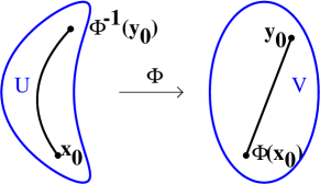
Figure 5: Computation of $\Phi^{-1}({\bf y}_{0})$.

In order to actually carry out this construction, we must be able to solve equations of the form

$$\Phi(\delta_{1},\cdots,\delta_{q})~{}=~{}(s_{1},\cdots,s_{q})$$

for any given sequence of $s_{j}$.

Lemma .

Let $\Phi:U\stackrel{{\scriptstyle\cong}}{{\longrightarrow}}V$ be an explicitly given diffeomorphism between open sets of ${\mathbb{R}}^{n}$ for any $n>0$, with $V$ convex. Then for any ${\bf y}_{0}\in V$ we can effectively compute the pre-image $\Phi^{-1}({\bf y}_{0})\in U$.

Proof.

(Compare Figure 5.) Choose an arbitrary point ${\bf x}_{0}\in U$ and draw a straight line

$$t~{}\mapsto{\bf y}(t)~{}=~{}(1-t)\Phi({\bf x}_{0})+t\,{\bf y}_{0}$$

from $\Phi({\bf x}_{0})$ to ${\bf y}_{0}$. Then the curve ${\bf x}(t)=\Phi^{-1}\big{(}{\bf y}(t)\big{)}$ in $U$ joints ${\bf x}_{0}$ to the required point $\Phi^{-1}({\bf y}_{0})$. This lifted curve satisfies a differential equation of the form

$$\Phi^{\prime}({\bf x})\,\frac{d{\bf x}}{dt}~{}~{}=~{}~{}\frac{d{\bf y}}{dt}~{}~{}=~{}~{}{\bf y}_{0}-\Phi({\bf x}_{0})~{}.$$

Here $\Phi^{\prime}$ is defined to be the $q\times q$ matrix of first partial derivatives, and $d{\bf x}/dt$ and $d{\bf y}/dt$ should be thought of as column vectors. Equivalently we can write

$$\frac{d{\bf x}}{dt}~{}~{}=~{}~{}\Phi^{\prime}(t)^{-1}\big{(}{\bf y}_{0}-\phi({\bf x}_{0})\big{)}~{},$$

where the right hand side can be explicitly computed. There exist standard packages for solving such systems of differential equations to any reasonable degree of accuracy. Therefore the curve ${\bf x}(t)$, and hence its endpoint $\Phi^{-1}({\bf y}_{0})$, can be effectively computed. ∎

In fact, for the Douady-Sentenac diffeomorphism, a straightforward use of Newton’s method in several variables converges readily, provided one chooses an appropriate starting point. For more general diffeomorphisms or poor choices of initial conditions, Newton’s method can behave very badly. While the local convergence of Newton’s method for such functions is well understood and goes back over a century (see [F]) and was greatly expanded by Kantorovič in the 1940s [K] (see also [D, Thm. 2.1], [HH, §2.8]), the global behavior even for diffeomorphisms is not currently understood.

4 The Algorithm.

Again we first consider the case of simple critical points, and suppose that some combinatorics ${\stackrel{{\scriptstyle\rightarrow}}{{m}}}=(m_{0},~{}m_{1},~{}\cdots,~{}m_{n})$ has been specified. Let $X_{n}$ be the space of all ${\stackrel{{\scriptstyle\rightarrow}}{{x}}}=(x_{0},\cdots,x_{n})$ with

$$0=x_{0}<x_{1}<\cdots<x_{n-1}<x_{n}=1~{},$$

and let $0<j_{1}<\ldots<j_{d-1}<n~{}$ be the indices for which $m_{j}$ is a local maximum or minimum. The pull-back transformation

$$T:X_{n}\to X_{n}$$

which is associated with ${\stackrel{{\scriptstyle\rightarrow}}{{m}}}$ can be described as follows. Given an arbitrary ${\stackrel{{\scriptstyle\rightarrow}}{{x}}}=(x_{0},\cdots,x_{n})$ in $X_{n}$, set $y_{j}=x_{m_{j}}$. According to Section 3, there is a unique map $f=f_{\stackrel{{\scriptstyle\rightarrow}}{{x}}}$ in $K_{\mathbb{R}}$-normal form with critical values $v_{i}=y_{j_{i}}$. The image $T({\stackrel{{\scriptstyle\rightarrow}}{{x}}})={\stackrel{{\scriptstyle\rightarrow}}{{x}}}^{\prime}$ is a new element of $X_{n}$ satisfying the equation

$$f(x^{\prime}_{j})=y_{j}\qquad{\rm for~{}all}~{}~{}~{}j~{}.$$

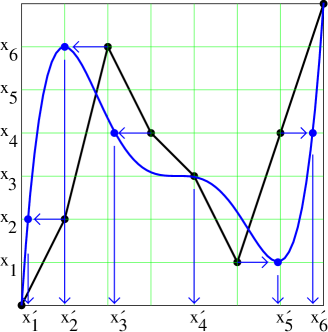
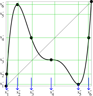
Figure 6: First two steps of the algorithm for the combinatorics ${\stackrel{{\scriptstyle\rightarrow}}{{m}}}=(0,2,6^{2},4,3^{3},1^{2},4,7)$. On the left: Start with the associated piecewise linear model map $f_{0}$, shown in black. The evenly spaced green grid line correspond to points $(x,y)$ with $x=x_{j}$ or $y=x_{j}$. Note that the “critical value vector” for $f_{0}$ is the 4-tuple ${\stackrel{{\scriptstyle\rightarrow}}{{v}}}_{0}=(x_{6},\,x_{3},\,x_{3},\,x_{1})$, since the point $(x_{4}^{\prime},\,x_{3})$ has been assigned local degree three. Let $f_{1}$, shown in blue, be the unique framed polynomial map with the same critical value vector. Corresponding to each critical or postcritical point $(x,y)=(x_{j},x_{m_{j}})$ on the graph of $f_{0}$, let $(x^{\prime}_{j},y_{j})$ be the unique point on the corresponding lap of $f_{1}$ with the same $y$-coordinate. Note in particular that each critical point of $f_{0}$ corresponds to a critical point of $f_{1}$. The correspondence $T:{\stackrel{{\scriptstyle\rightarrow}}{{x}}}\mapsto{\stackrel{{\scriptstyle\rightarrow}}{{x}}}^{\prime}$ is called the pull-back transformation. On the right: The green grid coordinates are now the points $(x,y)$ with $x=x^{\prime}_{j}$ or $y=x^{\prime}_{j}$. Let $f_{2}$ be the polynomial map with critical value vector $(x^{\prime}_{6},x^{\prime}_{3},x^{\prime}_{3},x^{\prime}_{1})$. Now for each $(x^{\prime}_{j},x^{\prime}_{m_{j}})$ let $(x^{\prime\prime}_{j},\,x^{\prime}_{m_{j}})$ be the point on the corresponding lap of $f_{2}$ with height $x^{\prime}_{m_{j}}$. Then the pull-back transformation sends ${\stackrel{{\scriptstyle\rightarrow}}{{x}}}^{\prime}$ to ${\stackrel{{\scriptstyle\rightarrow}}{{x}}}^{\prime\prime}$. Note that each $x^{\prime\prime}_{j}$ is fairly close to $x^{\prime}_{j}$, so that the iteration seems to be converging well.

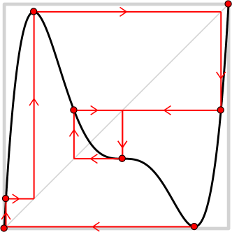
Figure 7: Showing the limiting map for the combinatorics $(0,2,6^{2},4,3^{3},1^{2},4,7)$ of Figure 6. (Here the last critical value is strictly positive, although very close to zero.) The mapping pattern is $~{}\underline{\underline{x_{5}}}\mapsto x_{1}\mapsto\underline{\underline{x_{2}}}\mapsto x_{6}\mapsto x_{4}\leftrightarrow\underline{\underline{\underline{x_{3}}}}$.

To see that ${\stackrel{{\scriptstyle\rightarrow}}{{x}}}^{\prime}$ is uniquely defined, first consider the $d-1$ critical indices $j_{i}$. Choose $x^{\prime}_{j_{i}}$ to be the corresponding critical point of $f$, so that

$$f(x^{\prime}_{j_{i}})={y_{j_{i}}}=v_{i}~{},\qquad{\rm as~{}required.}$$

Now consider the remaining indices $j$. The $d-1$ critical points of $f$ separate the graph of $f$ into $d$ monotone segments called laps. Since we require that $x^{\prime}_{0}<x^{\prime}_{1}<\cdots<x^{\prime}_{n}$, each of the remaining $x^{\prime}_{j}$ must belong to a well defined lap. Therefore, using the intermediate value theorem, $x^{\prime}_{j}$ is uniquely determined by its image $f(x^{\prime}_{j})=y_{j}$ within that lap. This completes the description of $T$ in the special case of simple critical points. A very similar argument applies in the more general case, as long as Condition (6) of Section 3 holds; see Figure 6. See Appendix A for a more detailed discussion.

If we can find a fixed point ${\stackrel{{\scriptstyle\rightarrow}}{{x}}}=T({\stackrel{{\scriptstyle\rightarrow}}{{x}}})$ for this transformation, then evidently the associated $f$ will be the desired critically finite polynomial which satisfies the identity

$$f(x_{j})~{}=~{}x_{m_{j}}~{}.$$

In particular, starting with any ${\stackrel{{\scriptstyle\rightarrow}}{{x}}}\in X_{n}$, if the successive iterated images $T^{\circ k}({\stackrel{{\scriptstyle\rightarrow}}{{x}}})$ converge to a limit in $X_{n}$, then the polynomial $f_{\infty}$ associated with this limit will be such a fixed point. In fact if the combinatorics satisfies all of our requirements (including the expansiveness condition), then such a unique limit always exists. A more detailed explanation follows.

Definition .

A Thurston map is an orientation preserving branched covering map from a topological 2-sphere onto itself which is “critically finite” in the sense that every branch point has a finite forward orbit. (It will be convenient to refer to the branch points as critical points.) If there are $n\geq 5$ postcritical points (and in many cases if there are $n=4$), Thurston defines the pull-back transformation on an associated Teichmüller space for the surface of genus zero with $n$ marked points, and proves that this transformation converges to a unique limit unless there is a well defined obstruction which prevents convergence. See [DH] for details.

As examples, flexible Lattès maps (see e.g. [M]) provide 1-parameter families of rational maps of arbitrarily high degree with 4 postcritical points, all in the same equivalence class as Thurston maps. Such examples cannot occur when there are 5 or more postcritical points.

Such a Thurston map is a topological polynomial if there is a marked branch point (corresponding to the point at infinity for an actual polynomial) which is fixed, and has no preimages other than itself. This special case is much easier to deal with. (Compare [BFH].) In particular, the only possible obstruction is a Levy cycle; the cases with $n\leq 4$ postcritical points present no problem. Such a topological polynomial can always be represented by a Hubbard tree, and there is no Levy cycle if and only if an appropriate expansiveness condition is satisfied. (Compare [BS] or [P2].)

By a real topological polynomial we will mean a piecewise monotone map from ${\mathbb{R}}/{\mathbb{Z}}$ to itself such that only zero maps to zero, with specified “critical points” satisfying the requirements of Condition (6) of Section 3. This is much easier to deal with than a complex topological polynomial. Each choice of combinatorics (whether or not the Expansiveness Condition 2 of Section 2 is satisfied) gives rise to a formal Hubbard tree contained in the real line, with its associated real topological polynomial. The Thurston algorithm for this real topological polynomial will converge to an actual polynomial having the specified combinatorics if and only if the expansiveness condition is satisfied. (Actually, we will see in Appendix B that there is a weaker form of convergence even without expansiveness.)

Of course we need an actual complex topological polynomial in order to apply Thurston’s convergence theorem. We will describe the construction of the complex topological polynomial from the real combinatorics in one typical example, leaving the general construction to the reader.

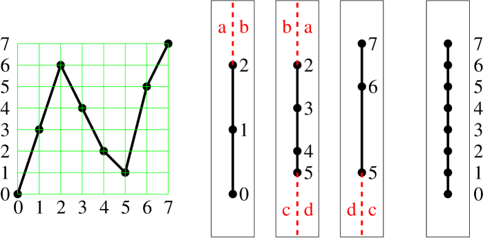
Figure 8: Construction of a branched covering of the sphere with combinatorics $(0,3,6,4,2,1,5,7)$.

Start with the piecewise linear model (Figure 8-left), with combinatorics

$$(0,\,3,\,6,\,4,\,2,\,1,\,5,\,7)~{}.$$

Step 1. For each of the three laps, choose a copy of ${\mathbb{C}}$ with the real axis vertical, as indicated schematically in the middle of the figure, and project each lap to the corresponding real axis. For each marked point on the lap, mark a corresponding point on this real axis, with height the associated $y$ value, but with label the associated $x$ value.

Next slit each of these copies of ${\mathbb{C}}$ along the dotted lines, and then paste the resulting boundary curves together in pairs; pasting side “a” to side “a” and so on. The result will be a connected simply connected surface $S$, which is homeomorphic to ${\mathbb{C}}$.

Step 2. Project $S$ onto another copy $S^{\prime}$ of ${\mathbb{C}}$, as represented on the right of the figure, where now the marked points are labeled by their $y$ values. Note that this projection is a branched covering, locally two-to-one at the branch points, which are labeled 2 and 5. Thus we have a branched covering $S\to S^{\prime}$.

Step 3. Finally identify $S$ with $S^{\prime}$ by choosing a homeomorphism $S\leftrightarrow S^{\prime}$ which sends the emphasized part of each real axis to the real axis, and sends each marked point to the point with the same label. Thus (after adding a point at infinity to each surface) we obtain the required map from a topological sphere to itself. As an example, the point labeled 1 on $S^{\prime}$ is identified with the point labeled 1 on $S$, and maps to the point labeled 3 on $S^{\prime}$.

The discussion would be similar for any example with distinct real critical points. The case with higher order critical points is more complicated, and can be dealt with more easily by using external rays in the complex plane. See for example [P1] and [P2].

Appendix A Implementing the method computationally

Implementation of the method is relatively straightforward, although there are a few issues which need a little care. For low degree polynomials with fairly tame combinatorics, all of the calculations can be done in standard double-precision. For polynomials of degree 6 or higher (and in some particular low-degree cases), calculations often require more digits in order to converge.

As an explicit example, for the combinatorics $(0,3,2,1,4)$ the method converges quite rapidly to the degree 3 limiting polynomial; see Figure 9. Using double precision (about 13 decimal digits), the method converges to within $6\times 10^{-6}$ in 5 steps, or better than $10^{-12}$ after 17 steps. For comparison, if we keep the combinatorics the same but change the first critical point to have local degree 4 and make the central fixed point have local degree 3 (that is, combinatorics $(0,3^{4},2^{3},1,4)$), the method requires much more precision to converge to the corresponding degree 7 polynomial. Using double-precision arithmetic, it converges to within $1.3\times 10^{-5}$ after 8 steps, but then loses precision, with the error oscillating between $2\times 10^{-4}$ and $7\times 10^{-6}$. Increasing the precision to 20 digits gives better than $10^{-7}$ in 10 steps. One needs at least 27 digits of precision to get a limiting map good to within $10^{-12}$ (in 19 steps).

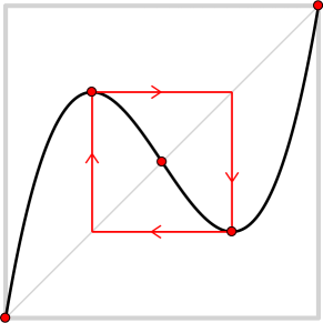
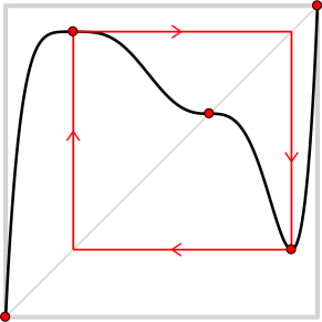
Figure 9: Two limiting polynomials, both with topological combinatorics $(0,3,2,1,4)$ (that is, the same piecewise-linear map). The polynomial on the left is cubic with simple critical points, while the polynomial on the right has degree 7 and combinatorics $(0,3^{4},2^{3},1,4)$.

We have written an implementation for arbitrary combinatorics and degree in Maple, although it would be straightforward to port this to many other languages, as long as the language supports multiple-precision arithmetic.

Implementation

Naturally, it is important to begin with combinatorics that are topologically possible and fully describe the situation, as described in Section 2.

We insist that the framing points ($x=0$ and $x=1$ for a map in $K_{\mathbb{R}}$ form) must be specified as part of the combinatorics. For polynomials of odd degree, we assume that the two end points are either fixed or form a period 2 cycle, while for even degree we assume $x=0$ is fixed and $x=1$ is the preimage of $x=0$. The other even degree case is easily obtained from this by a change of coordinates.

In the discussion below, we will use $x_{m}^{[\ell]}$ to denote the location of the $m$th marked point at the $\ell$th step of the process. We will also use $c_{j}^{[\ell]}$ to denote the $j$th critical point (which is, of course, one of the $x_{m}^{[\ell]}$). When the particular step is irrelevant or apparent, we may omit the superscript.

We perform the following steps:

1. Initialization. From the combinatorics (see Section 2), the indices corresponding to critical points can be inferred if local degrees are not explicitly specified. (As noted in §2, when local degrees are not specified, we assume that all critical points have local degree 2 and all other points are regular points.) Since the critical points are not required to be simple, we will have $r$ distinct critical points $(c_{1},c_{2},\ldots,c_{r})$ and $r$ (not necessarily distinct) critical values $(v_{1},\ldots,v_{r})$.

   Further, the laps can be determined just by inspection of the given combinatorics, with laps bounded by each turning point. Critical points of odd degree can be ignored when defining laps, because they do not affect the covering properties of the map. Here, because we will need to solve numerically for the two framing points, it is important to temporarily allow the initial and final laps to extend sufficiently far to the left or right; it is simplest to take them to be bounded by $\pm\infty$.

   As initial values for the marked points, we choose ${x_{1}^{[0]},x_{2}^{[0]},\ldots,x_{n-1}^{[0]}}$ to be equally spaced between $x_{0}=0$ and $x_{n}=1$, and take the initial map $f_{0}$ to be the piecewise linear map obeying the given combinatorics.

2. Mapmaking. Given a map $f_{\ell-1}$, the first step of the iterative process is to choose $\breve{f_{\ell}}$ with the correct critical values: we must determine a map $\breve{f_{\ell}}$ with critical points $\breve{c_{j}}^{[\ell]}$ corresponding to the desired critical values. That is,

   $$\breve{f_{\ell}}(\breve{c_{j}}^{[\ell]})=x^{[\ell-1]}_{m_{j}}=v^{[\ell]}_{j},\quad\text{where $m_{j}$ is the index of the image of $\breve{c_{j}}^{[\ell]}$}\,.$$ (A.1)

   This is done by inverting the map $\Phi$ of Section 3. Given the critical-value vector $(v_{1},v_{2},\ldots,v_{r})$, we compute the successive distances

   $$s_{1}=|v_{2}-v_{1}|,\;s_{2}=|v_{3}-v_{2}|,\;\ldots\,,\;s_{r-1}=|v_{r}-v_{r-1}|,$$

   and then use Newton’s method to find $\delta_{i}$ so that

   $$(\delta_{1},\ldots,\delta_{r-1})\approx\Phi^{-1}(s_{1},\ldots,s_{r-1}).$$

   While Newton’s method can be unpredictable, a good initial choice is to use a scaled version of the critical points for the corresponding Chebyshev polynomial of the first kind. Specifically, take

   $$\rho_{j}=\frac{2}{4^{1/r}}\Bigl{(}\cos\bigl{(}j\pi/r\bigr{)}-\cos\bigl{(}(j-1)\pi/r\bigr{)}\Bigr{)}$$

   as initial point for the Newton iteration $\vec{\rho}\,\mapsto\,\vec{\rho}-\bigl{(}\Phi^{\prime}(\vec{\rho})\bigr{)}^{-1}\,\Phi(\vec{\rho})$; see Appendix A. This yields a map $\breve{f_{\ell}}$ with the desired critical values to within any given tolerance, although the critical points $\breve{c_{j}}$ of $\breve{f_{\ell}}$ will not necessarily be in $[0,1]$.

3. Normalization. In order to have a map $f_{\ell}\in K_{\mathbb{R}}$, we first need to determine the framing points by solving the appropriate framing condition. We find $A$ in the initial lap and $B$ in the final lap such that $\breve{f_{\ell}}(A)$ and $\breve{f_{\ell}}(B)$ are either $0$ or $1$ as given by the combinatorics. Then we let $f_{\ell}=\breve{f_{\ell}}\circ\mu$ and $c_{j}=\mu(\breve{c_{j}})$, where $\mu$ is the appropriate linear map with $\mu(A)=0$, $\mu(B)=1$.

   As the degree grows, numerical uncertainty in the framing points can cause the resulting map $f_{\ell}$ to fail to achieve the desired numerical tolerances, in which case we repeat (1) with increased precision, starting from the $c_{j}$ after normalization, then normalize the resulting map again.

   

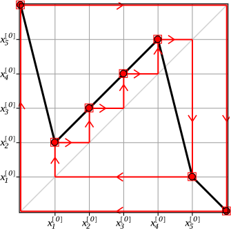
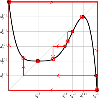
   Figure 10: The piecewise linear map $f_{0}$ (on the left) and the first step $f_{1}$ (on right) for combinatorics $(6,2^{4},3,4,5,1,0)$. Here (and in Figure 11), the image of a marked point is indicated by an open square on the graph. When passing from the piecewise linear $f_{0}$ to the polynomial $f_{1}$, observe that while $f_{1}(x_{k}^{[1]})=f_{0}(x_{k}^{[0]})$, the points $x_{k}$ in the domain have all moved significantly. Further, at step 1, the dynamics are significantly off (the image of each $x_{k}^{[1]},1\leq k<5$ is too far to the left).

4. Pullback. We now have the unique map $f_{\ell}\in K_{\mathbb{R}}$ which satisfies Equation (A.1); this is the map $f_{\ell}$ on $[0,1]$ with the specified critical values $v_{j}^{[\ell]}$ and known critical points $c_{j}^{[\ell]}$. Since each of these points $c_{j}^{[\ell]}$ is a point $x_{m_{j}}^{[\ell]}$, we just need to find the remaining noncritical $x_{k}^{[\ell]}$. For each of these, we solve (numerically)

   $$f_{\ell}(x_{k}^{[\ell]})=x_{m_{k}}^{[\ell-1]},$$

   where $m_{k}$ is the index of the image of $x_{k}$ given by the combinatorics and $x_{k}^{[\ell]}$ lying in the appropriate lap, as discussed in Section 4. See Figures 10 and 11.

5. Goodness of fit. To measure how well $f_{\ell}$ satisfies the conditions, calculate the distance $\epsilon_{\ell}$ between the images $f_{\ell}(x_{k}^{[\ell]})$ and the corresponding points in the orbit $y_{k}^{[\ell]}=x_{m_{k}}^{[\ell]}$, that is,

   $$\epsilon_{\ell}=\frac{1}{n}\Bigl{(}{\sum_{j=0}^{n}\left.f_{\ell}(x_{k}^{[\ell]})^{2}-(y_{k}^{[\ell]})^{2}\right.}\Bigr{)}^{1/2}\,.$$

   If $\epsilon_{\ell}$ is not sufficiently small, increment $\ell$ and repeat steps (1)–(4).

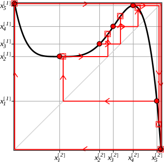
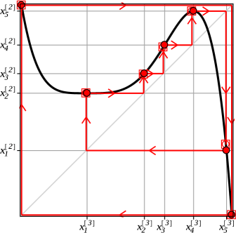
Figure 11: Steps 2 and 3 of the method for the combinatorics of Figure 10. Note that Step 3 (on the right) is becoming close to the desired limit dynamics (although only at step 11 is the error within $10^{-5}$).

As noted earlier, the global behavior of Newton’s method can be unpredictable, even for diffeomorphisms. Hence, to determine a polynomial with the given critical values in step (1), we need to select an appropriate initial approximation.

Since Chebyshev polynomials have distinct critical points and only two critical values, we can easily use them to construct polynomials with critical points $c_{j}$ for which $\Phi(\rho_{1},\ldots,\rho_{r-1})=(1,1,\ldots,1)$ (with $|c_{j}-c_{j+1}|=\rho_{j}$). Assuming the following conjecture, Newton’s method will always converge to the desired solution when started from such an initial condition.

Conjecture .

Given $(s_{1},\ldots,s_{r-1})$ with $0<s_{j}\leq 1$ for all $j$, suppose that $(\rho_{1},\ldots,\rho_{r-1})$ is chosen so that $\Phi(\rho_{1},\ldots,\rho_{r-1})=(\sigma_{1},\ldots,\sigma_{r-1})$, with $s_{j}\leq\sigma_{j}\leq 1$ for all $j$. Then Newton’s method, when started with $(\rho_{1},\ldots,\rho_{r-1})$ as the initial condition, will converge to the desired solution $(\delta_{1},\ldots,\delta_{r-1})=\Phi^{-1}(s_{1},\ldots,s_{r-1})$.

While we haven’t quite been able to establish Appendix A, observe that all entries of the first derivative matrix $\Phi^{\prime}$ are non-negative in this region, as are the partial derivatives of each entry. These properties certainly simplify the situation, and in most cases Newton’s method decreases monotonically in each coordinate towards $(\delta_{1},\ldots,\delta_{r-1})$.

Even without assuming the conjecture, one can apply a modified version of Newton’s method to ensure convergence (see [D, ch.3], for example). We have not found a situation in which this was necessary.

Appendix B Further Examples: The Non-Expansive Case

In this section, after presenting another typical example, we move to examples with non-expansive combinatorics. In the non-expansive case, the Thurston algorithm converges only in a much weaker sense, as follows from a theorem of Selinger [S].

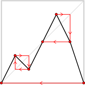
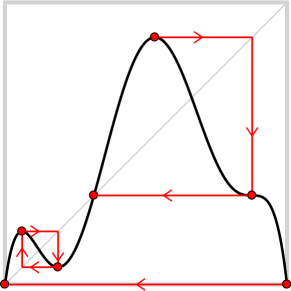
Figure 12: On the left is the PL model for the combinatorics $(0,2,1,3,5,3^{3},0)$, with $~{}~{}\underline{\underline{x_{1}}}\leftrightarrow\underline{\underline{x_{2}}}$ and $\underline{\underline{x_{4}}}\mapsto\underline{\underline{\underline{x_{5}}}}\mapsto x_{3}\,\rotatebox[origin={c}]{90.0}{\large$\circlearrowleft$}\,$. On the right is the corresponding polynomial map of degree six.

Figure 12 shows an example which satisfies all six of the conditions of Section 2. For such examples, all of the marked points will remain distinct in the limit. On the other hand, Figure 13 shows an example of combinatorics which violates the expansiveness condition 2 of Section 2: no forward image of the interval $[2,3]$ contains a critical point. Applying the Thurston algorithm to this example, the interval $[2,3]$ shrinks to a point, as shown in the graph to the right in Figure 13, so that the combinatorics becomes simpler.

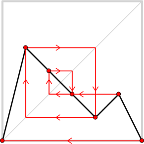
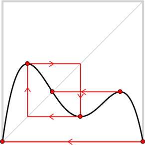
Figure 13: On the left is the PL model for combinatorics $(0,4,3,2,1,2,0)$ with mapping pattern $\underline{\underline{x}}_{1}\leftrightarrow\underline{\underline{x_{4}}}~{},\quad\underline{\underline{x_{5}}}\mapsto x_{3}\leftrightarrow x_{2}$. On the right is the corresponding polynomial map of degree four. Here the interval $[2,3]$ of the PL model on the left has shrunk to the circled fixed point, and the combinatorics has simplified to $(0,3,2,1,2,0)$, with mapping pattern $~{}~{}\underline{\underline{x_{1}}}\leftrightarrow\underline{\underline{x_{3}}}~{},\quad\underline{\underline{x_{4}}}\mapsto x_{2}\,\rotatebox[origin={c}]{90.0}{\large$\circlearrowleft$}\,$.

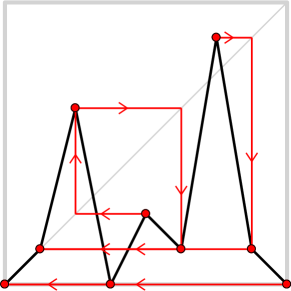
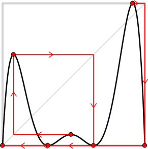
Figure 14: On the left: a piecewise linear map with combinatorics $(0,1,5,0,2,1,7,1,0)$. Here every critical orbit ends either at the fixed point zero or at the fixed point with number one. However the initial interval $[0,1]$ and the final interval $[7,8]$ fail to be expansive; so on the right the associated polynomial map is simpler, with combinatorics $(0,4,0,1,0,6,0)$. The mapping pattern in the limit is $\underline{\underline{x_{3}}}\mapsto\underline{\underline{x_{1}}}\mapsto\underline{\underline{x_{4}}}\mapsto x_{0}\,\rotatebox[origin={c}]{90.0}{\large$\circlearrowleft$}\,$,   $\underline{\underline{x_{5}}}\mapsto x_{6}\mapsto x_{0}\,\rotatebox[origin={c}]{90.0}{\large$\circlearrowleft$}\,$, and $~{}~{}\underline{\underline{x_{2}}}\mapsto x_{0}\,\rotatebox[origin={c}]{90.0}{\large$\circlearrowleft$}\,$,   with all critical orbits ending at the repelling fixed point $x_{0}$.

Figure 14 shows a similar example. Here both of the intervals $[0,1]$ and $[7,8]$ collapse to points under the Thurston algorithm, so that again the final polynomial map is simpler than the original PL map.

These examples illustrate the following statement, which follows relatively easily from the work of Nikita Selinger [S, Proposition 6.2]. We want to thank Kevin Pilgrim, Thomas Sharland, as well as Selinger himself, for pointing this out to us.

Assertion .

Even if the given combinatorics does not satisfy the expansiveness condition, the successive polynomial approximations given by the Thurston algorithm will still converge locally uniformly to a critically finite polynomial. However this limit polynomial will have simpler combinatorics. More precisely, every edge of the piecewise linear model which is not expansive will collapse to a point.

We will not attempt to provide further details, but encourage the interested reader to study Selinger’s paper.

Appendix C Coefficients.

Table C.1: The coefficients for the polynomials in several of the figures, and the corresponding error estimates, evaluated as $\tfrac{1}{n}\sqrt{{\sum(f(x_{i})-y_{i})^{2}}}$ where the $x_{i}$ are the marked points, and $y_{i}$ is the desired value for $f(x_{i})$. The error estimates marked with * represent initial steps for the Thurston algorithm, while the remaining estimates represent estimates after many steps of the algorithm. Note that the coefficients for Figure 6 are beginning to converge towards the coefficients for Figure 7. Similarly, the coefficients for Figures 10(r) and 11 are beginning to converge towards the Thurston limit.

Fig.	polynomial	error bound	Iter
2	$7.121692805x-17.64597623x^{2}+11.52428342x^{3}$	$1.24\times 10^{-8}$	20
6(l)	$15.332055x-92.795911x^{2}+225.00679x^{3}-242.71367x^{4}+96.170733x^{5}$	$0.037^{*}$	1
6(r)	$18.069912x-112.83091x^{2}+273.38011x^{3}-292.41971x^{4}+114.80059x^{5}$	$0.0038^{*}$	2
7	$18.163069x-113.72167x^{2}+276.22221x^{3}-296.09149x^{4}+116.42789x^{5}$	$1.84\times 10^{-6}$	13
9(l)	$6x-15x^{2}+10x^{3}$	$1\times 10^{-13}$	14
9(r)	$0.20557075x-181.7478872x^{2}+855.1404749x^{3}-2244.547436x^{4}+3255.216137x^{5}-2427.230116x^{6}+723.9632564x^{7}$	$4.13\times 10^{-8}$	18
10(r)	$1-8.73730x+44.7494x^{2}-110.928x^{3}+130.960x^{4}-57.0449x^{5}$	$0.0791^{*}$	1
11(l)	$1-5.10905x+28.0816x^{2}-74.57010x^{3}+93.9995x^{4}-43.4011x^{5}$	$0.0144^{*}$	2
11(r)	$1.-5.82395x+31.5803x^{2}-82.7518x^{3}+102.974x^{4}-46.9785x^{5}$	$0.0021^{*}$	3
12(r)	$7.494214522x-97.01797994x^{2}+457.9211574x^{3}-913.0123135x^{4}+811.6279094x^{5}-267.0129879x^{6}$	$3.54\times 10^{-9}$	25
13(r)	$7.45977893x-32.0733758x^{2}+47.0904007x^{3}-22.4768041x^{4}$	$5.49\times 10^{-9}$	36
14(r)	$20.15184092x-208.9317665x^{2}+827.5262978x^{3}-1559.747539x^{4}+1400.650082x^{5}-479.6489149x^{6}$	$6.34\times 10^{-8}$	12

Table C.1: Continued from previous page

References

- [Ba-N] L. Bartholdi, V. Nekrashevych, Thurston equivalence of topological polynomials. Acta Math. 197 (2006) 1–51. doi:10.1007/s11511-006-0007-3. MR 2285317
- [Ba] L. Bartholdi, IMG, Computations with iterated monodromy groups, a GAP package, version 0.1.1. laurentbartholdi.github.io/img/
- [BFH] B. Bielefeld, Y. Fisher, and J. H. Hubbard, The classification of critically preperiodic polynomials as dynamical systems. J. Amer. Math. Soc. 5 (1992) 721–762. doi:10.2307/2152709. MR 1149891.
- [BKM] A. Bonifant, J. Kiwi, and J. Milnor, Cubic polynomial maps with periodic critical orbit, II. Conf. Geom. Dyn. 14 (2010) 68–112. doi:10.1090/S1088-4173-10-00204-3. MR 2600536
- [BMS] A. Bonifant, J. Milnor, and S. Sutherland, The W. Thurston Algorithm for Real Quadratic Rational Maps, arXiv:2009.10147 [] [math.DS] (2020).
- [BS] H. Bruin and D. Schleicher, Admissibility of kneading sequences and structure of Hubbard trees for quadratic polynomials. J. London Math. Soc. 78 (2008) 502–522. doi:10.1112/jlms/jdn033. MR 2439637.
- [Ch] A. Chéritat, Tan Lei and Shishikura’s example of non-mateable degree 3 polynomials without a Levy cycle, Ann. Fac. Sc. Toulouse 21 (2012) 935–980. doi:10.5802/afst.1358. MR 3088263
- [D] P. Deuflhard, Newton methods for nonlinear problems: Affine invariance and adaptive algorithms, Springer Ser. in Comp. Math. 35. Springer-Verlag, 2011. doi:10.1007/978-3-642-23899-4. MR 2893875
- [DH] A. Douady and J. H. Hubbard, A proof of Thurston’s topological characterization of rational functions, Acta Math. 171 2 (1993) 263–297. doi:10.1007/BF02392534. MR 1251582
- [F] H. B. Fine, On Newton’s method of approximation, Proc. Nat. Acad. Sci. USA 2 (1916) 546–552. doi:10.1073/pnas.2.9.546.
-
[H-He]
S. Hruska-Boyd, C. Henriksen,
The Medusa algorithm for polynomial matings,
Conf. Geom. Dyn. 16 (2012) 161–183.
doi:10.1090/S1088-4173-2012-00245-7. MR 2943594
The code was ported to standard C++ by Chris King, dhushara.com/DarkHeart/ - [HH] B. B. Hubbard and J. H. Hubbard, “Vector calculus, linear algebra, and differential forms: a unified approach”, 4th ed. Matrix Editions, Ithaca NY, 2009. MR 1657732
- [HS] J. H. Hubbard and D. Schleicher, The spider algorithm.“Complex Dynamical Systems” (Cincinnati, OH, 1994) Proc. Sympos. Appl. Math., 49 Amer. Math. Soc., Providence, RI, 1994, pp. 155–180. doi:10.1090/psapm/049/1315537. MR 1315537
- [H] A. Hurwitz, Ueber Riemann’sche Flächen mit gegebenen Verzweigungspunkten, Math. Ann. 39 (1891) 1–61. doi:10.1007/BF01199469. MR 1510692
- [J] W. Jung, The Thurston algorithm for quadratic matings. arXiv:1706.04177 [].
- [K] L. V. Kantorovič, On Newton’s method (Russian), Trudy Mat. Inst. Steklov. 28 (1949) 104–144. MR 0038560.
- [M] J. Milnor, On Lattès maps. “Dynamics on the Riemann Sphere”, P. Hjorth and C. L. Petersen editors, Eur. Math. Soc. 2006, pp. 9–43. MR 2348953
- [MTr] J. Milnor and C. Tresser, On entropy and monotonicity for real cubic maps (with an appendix by A. Douady and P. Sentenac). Comm. Math. Phys. 209 (2000) 123–178. doi:10.1007/s002200050018. MR 1736945
- [P1] A. Poirier, Critical portraits for postcritically finite polynomials. Fund. Math. 203 (2009) 107–163. doi:10.4064/fm203-2-2. MR 2496235
- [P2] A. Poirier, Hubbard Trees. Fund. Math. 208 (2010) 193–248. doi:10.4064/fm208-3-1. MR 2650982
- [S] N. Selinger, Thurston’s pullback map on the augmented Teichmüller space and applications. Invent. Math. 189 (2012) 111–142. doi:10.1007/s00222-011-0362-3. MR 2929084
- [T] D. Thurston, From rubber bands to rational maps: a research report, Res. Math. Sci. 3 (2016) #15. doi:10.1186/s40687-015-0039-4. MR 3500499