Spin density wave and electron nematicity in magic-angle twisted bilayer graphene

Abstract

We study theoretically many-body properties of magic-angle twisted bilayer graphene for different doping levels. Our investigation is focused on the emergence, stability, and manifestations of nematicity of the ordered low-temperature electronic state. It is known that, at vanishing interactions, the low-energy spectrum of the system studied consists of four almost-flat almost-degenerate bands. Electron-electron repulsion lifts this degeneracy. To account for such an interaction effect, a numerical mean-field theory is used. Assuming that the ground state has spin-density-wave-like order, we introduce a multicomponent order parameter describing spin magnetization. Our simulations show that the order parameter structure depends on the doping level. In particular, doping away from the charge neutrality point reduces the rotational symmetry of the ordered state, indicating the appearance of an electron nematic state. Manifestations of the nematicity can be observed in the spatial distribution of the spin magnetization within a moiré cell, as well as in the single-electron band structure. The nematicity is the strongest at half-filling (two extra electron or holes per supercell). We argue that nematic symmetry breaking is a robust feature of the system ground state, stable against model parameters variations. Specifically, it is shown that, away from the charge neutrality point, it persists for all three parametrizations of the interlayer hopping amplitudes discussed in the paper. Obtained theoretical results are consistent with the available experimental data.

I Introduction

Discovery of many-body insulating states Cao et al. (2018a) and superconductivity Cao et al. (2018b) in the so-called magic-angle twisted bilayer graphene Rozhkov et al. (2016) (MAtBLG) has triggered an avalanche of both theoretical Wu et al. (2018); Liu et al. (2018); Padhi et al. (2018); Guo et al. (2018); Ochi et al. (2018); Sboychakov et al. (2019); González and Stauber (2019); Huang et al. (2019); Lian et al. (2019); Roy and Juričić (2019); Seo et al. (2019); Fernandes and Venderbos (2019); Cea et al. (2019); Cea and Guinea (2020) and experimental Qiao et al. (2018); Lu et al. (2019); Choi et al. (2019); Kerelsky et al. (2019); Liu et al. (2019); Utama et al. (2019); Xie et al. (2019); Wong et al. (2019); Tomarken et al. (2019); Cao et al. (2020); Jiang et al. (2019) studies of this material. The MAtBLG has a twist angle $\theta_{c}\sim 1^{\circ}$ and it is characterized by a superstructure with a large supercell containing several thousand carbon atoms. Single-electron states of MAtBLG form four weakly dispersive (almost flat) low-energy bands Lopes dos Santos et al. (2012); San-Jose et al. (2012); Suárez Morell et al. (2010); Sboychakov et al. (2015) (these flat bands were recently visualized by ARPES in Ref. Utama et al., 2019). Measurements Cao et al. (2018a, b) of the conductivity $\sigma$ of MAtBLG versus doping $n$ reveal several conductivity minima at doping values $n/(n_{s}/4)\equiv\nu=0,\,\pm 2,\,\pm 3,\,\pm 4$, where the concentration $n_{s}$ corresponds Cao et al. (2018a, b) to four electrons per supercell. Observation of the “missing” conductivity minima at $\nu=\pm 1$ was later reported in Ref. Lu et al., 2019. Besides these findings, Ref. Cao et al., 2018b reported superconductivity domes near $\nu=-2$. Superconductivity domes near $\nu=-2$, $\nu=0$, and $\nu=\pm 1$ were also found Lu et al. (2019).

Theoretically, conductivity minima at $\nu=\pm 4$ can be understood in terms of single-electron physics Cao et al. (2018a). However, the minima at $\nu=\pm 1,\,\pm 2,\,\pm 3$ cannot be explained within single-particle theory, and the effects of interactions should be taken into account. The nature of the insulating states in MAtBLG was considered in several papers Padhi et al. (2018); Ochi et al. (2018); Liu et al. (2018); Huang et al. (2019); Seo et al. (2019); Sboychakov et al. (2019). Different types of spin density wave (SDW) states Liu et al. (2018); Huang et al. (2019); Sboychakov et al. (2019), ferromagnetic state Seo et al. (2019), and other symmetry broken phases Cea and Guinea (2020) have been proposed to be the ground state of the system. Potential mechanisms of the superconductivity (phonons Wu et al. (2018); Lian et al. (2019), electronic correlations Guo et al. (2018); Liu et al. (2018); González and Stauber (2019); Huang et al. (2019); Roy and Juričić (2019)) as well as various symmetries of the superconducting order parameters have been considered.

Neglecting the possibility of superconducting ordering, in a previous work Sboychakov et al. (2019), we assumed the multicomponent SDW to be the ground state of MAtBLG in the doping range $-4<\nu<4$. The structure of the SDW order parameter, as well as the form of the renormalized low-energy spectrum, was calculated Sboychakov et al. (2019) for different doping levels within the framework of a numerical mean-field approach. This allowed us to explain the appearance of conductivity minima at integer valued ratio $\nu$, consistent with experiments Cao et al. (2018a, b); Lu et al. (2019).

Since doping affects the mean-field band structure, the dependence of the density of states (DOS) $\rho$ versus the single-electron energy $E$ is sensitive to the doping level of the MAtBLG sample. This theoretical observation Sboychakov et al. (2019) is supported by recent STM measurements Wong et al. (2019); Xie et al. (2019); Choi et al. (2019); Kerelsky et al. (2019).

Further, we observed numerically Sboychakov et al. (2019) that, at sufficiently strong doping, the point symmetry of the electronic state reduces from $C_{6}$ (full hexagonal symmetry) down to $C_{2}$, giving rise to electron nematic state. References Choi et al., 2019; Kerelsky et al., 2019; Cao et al., 2020; Jiang et al., 2019 published claims of the experimental nematicity observations in MAtBLG samples.

The striking agreement between our conclusions Sboychakov et al. (2019) and several independent experimental measurements testifies in favor of the developed theoretical approach. To build up upon this success, here we extend the study of Ref. Sboychakov et al., 2019. In this paper we focus on the emergence, stability and manifestations of the electronic nematicity, demonstrating that nematic symmetry breaking is a robust feature of the MAtBLG, stable against model modifications, such as alterations of the interlayer hopping amplitudes. We will also argue that the nematicity affects not only the spatial distribution of the spin magnetization, but the single-electron spectrum as well. Experimental implications of these findings are discussed.

The paper is organized as follows. In Section II the geometry of the twisted bilayer graphene (tBLG) is outlined. In Section III we formulate our electronic model and analyze the single-particle spectrum of the MAtBLG for three different parametrizations of the interlayer hopping amplitudes. We also present the general form of our multicomponent SDW order parameter in this Section. In Section IV we analyze the spatial distribution of the SDW order parameter for different doping levels, while in Section V we consider the properties of the renormalized low-energy spectrum. Discussion of the results obtained and the conclusions are given in Section VI. Details of the numerical procedure used for the calculations of the SDW order parameter are described in the Appendix.

II Geometry of twisted bilayer graphene

In this Section we present some basic facts about the geometry of twisted bilayer graphene, which are important for further consideration (for more details, see, e.g., review papers Mele, 2012; Rozhkov et al., 2016). Each graphene layer in tBLG has a hexagonal crystal structure consisting of two triangular sublattices ${\cal A}$ and ${\cal B}$. The coordinates of atoms in layer $1$ on sublattices ${\cal A}$ and ${\cal B}$ are

$$\mathbf{r}_{\mathbf{n}}^{1{\cal A}}=\mathbf{r}_{\mathbf{n}}^{1}\equiv n\mathbf{a}_{1}+m\mathbf{a}_{2}\,,\;\;\mathbf{r}_{\mathbf{n}}^{1{\cal B}}=\mathbf{r}_{\mathbf{n}}^{1}+\bm{\delta}\,,$$ (1)

where $\mathbf{n}=(n,\,m)$ is an integer-valued vector,

$$\mathbf{a}_{1,2}=a(\sqrt{3},\mp 1)/2$$ (2)

are the primitive vectors, $\bm{\delta}=(\mathbf{a}_{1}+\mathbf{a}_{2})/3=a(1/\sqrt{3},0)$, and $a=2.46$ Å is the lattice constant of graphene. Atoms in layer $2$ are located at

$$\mathbf{r}_{\mathbf{n}}^{2{\cal B}}=\mathbf{r}_{\mathbf{n}}^{2}\equiv d\mathbf{e}_{z}+n\mathbf{a}_{1}^{\prime}+m\mathbf{a}_{2}^{\prime}\,,\quad\mathbf{r}_{\mathbf{n}}^{2{\cal A}}=\mathbf{r}_{\mathbf{n}}^{2}-\bm{\delta}^{\prime}\,,$$ (3)

where $\mathbf{a}_{1,2}^{\prime}$ and $\bm{\delta}^{\prime}$ are the vectors $\mathbf{a}_{1,2}$ and $\bm{\delta}$, rotated by the twist angle $\theta$. The unit vector along the $z$-axis is $\mathbf{e}_{z}$, the interlayer distance is $d=3.35$ Å. The limiting case $\theta=0$ corresponds to the AB stacking.

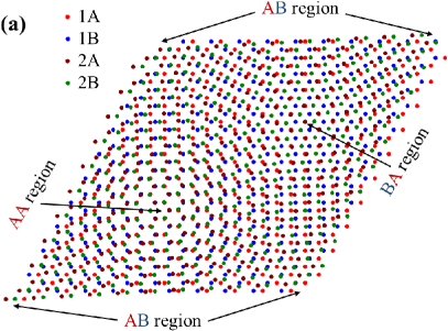
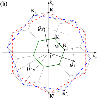
Figure 1: (a) The superlattice cell of the tBLG structure with $m_{0}=10$, $r=1$ ($\theta\cong 3.15^{\circ}$). Regions with almost AA, AB, and BA stackings are indicated by arrows. (b) Brillouin zones of layers 1 and 2 (big red and blue hexagons), as well as the Brillouin zone of the superlattice (small thick green hexagon) of the structure $m_{0}=1$, $r=1$ ($\theta\cong 21.79^{\circ}$). Reciprocal vectors of the superlattice, $\bm{{\cal G}}_{1,2}$, Dirac points of layers 1 and 2, $\mathbf{K}$, $\mathbf{K}^{\prime}$, $\mathbf{K}_{\theta}$, and $\mathbf{K}^{\prime}_{\theta}$, as well as symmetrical points of the reduced Brillouin zone ($\bm{\Gamma}$, $\mathbf{M}$, $\mathbf{K}_{1,2}$) are also shown.

Twisting produces moiré patterns Rozhkov et al. (2016), which can be seen as alternating dark and bright regions in STM images. Measuring the moiré period $L$, one can extract the twist angle according to the formula $L=a/[2\sin(\theta/2)]$. Moiré patterns exist for arbitrary twist angles. However, if the twist angle satisfies the relationship

$$\cos\theta=\frac{3m_{0}^{2}+3m_{0}r+r^{2}/2}{3m_{0}^{2}+3m_{0}r+r^{2}}\,,$$ (4)

where $m_{0}$ and $r$ are co-prime positive integers, a superstructure emerges, and a tBLG sample splits into a periodic lattice of finite supercells. Many theoretical papers assume the twist angle to be the commensurate one, since only in this case one can work with Bloch waves and introduce the quasimomentum. For the commensurate structure described by $m_{0}$ and $r$, the superlattice vectors are

$$\mathbf{R}_{1}=m_{0}\mathbf{a}_{1}+(m_{0}+r)\mathbf{a}_{2},\,\mathbf{R}_{2}=-(m_{0}+r)\mathbf{a}_{1}+(2m_{0}+r)\mathbf{a}_{2},$$ (5)

if $r\neq 3n$ ($n$ is an integer), or

$$\mathbf{R}_{1}=(m_{0}+n)\mathbf{a}_{1}+n\mathbf{a}_{2},\,\mathbf{R}_{2}=-n\mathbf{a}_{1}+(m_{0}+2n)\mathbf{a}_{2},$$ (6)

if $r=3n$. The number of graphene unit cells inside a supercell is

$$N_{\rm sc}=(3m_{0}^{2}+3m_{0}r+r^{2})/g$$ (7)

per layer. The parameter $g$ in the latter expression is equal to unity when $r\neq 3n$. Otherwise, it is $g=3$.

Note that, in the general case, the superlattice cell is greater in size than the moiré cell Lopes dos Santos et al. (2012); Rozhkov et al. (2016). More precisely, the superlattice cell of the structure with $m_{0}$ and $r$ contains $r^{2}$ moiré cells if $r\neq 3n$, or $r^{2}/3$ moiré cells otherwise. The arrangements of atoms in moiré cells constituting the superlattice cell are slightly different from each other. Only when $r=1$, the superlattice cell coincides with the moiré cell. In the present paper we consider only such structures. When $\theta$ is small enough, the superlattice cell can be approximately described as consisting of regions with almost AA, AB, and BA stackings Lopes dos Santos et al. (2012); Rozhkov et al. (2016). To illustrate this fact, in Fig. 1(a) we present the supercell of the tBLG structure with $m_{0}=10$, $r=1$ (these values of $m_{0}$ and $r$ correspond to $\theta\cong 3.15^{\circ}$).

Let us now consider what happens in momentum space. The reciprocal lattice primitive vectors for layer 1 (layer 2) are denoted by $\mathbf{b}_{1,2}$ ($\mathbf{b}_{1,2}^{\prime}$). For layer 1 one has

$$\mathbf{b}_{1,2}=(2\pi/\sqrt{3},\mp 2\pi)/a\,,$$ (8)

while $\mathbf{b}_{1,2}^{\prime}$ are connected to $\mathbf{b}_{1,2}$ by a rotation of an angle $\theta$. Using the notation $\bm{{\cal G}}_{1,2}$ for the primitive reciprocal vectors for the superlattice, the following identities in reciprocal space are valid:

$$\mathbf{b}_{1}^{\prime}=\mathbf{b}_{1}+r(\bm{{\cal G}}_{1}+\bm{{\cal G}}_{2})\,,\;\mathbf{b}_{2}^{\prime}=\mathbf{b}_{2}-r\bm{{\cal G}}_{1}\,,$$ (9)

if $r\neq 3n$, or

$$\mathbf{b}_{1}^{\prime}=\mathbf{b}_{1}+n(\bm{{\cal G}}_{1}+2\bm{{\cal G}}_{2})\,,\;\mathbf{b}_{2}^{\prime}=\mathbf{b}_{2}-n(2\bm{{\cal G}}_{1}+\bm{{\cal G}}_{2})\,,$$ (10)

if $r=3n$.

Each graphene layer in tBLG has a hexagonal-shaped Brillouin zone. The Brillouin zone of the layer $2$ is rotated in momentum space with respect to the Brillouin zone of layer $1$ by the twist angle $\theta$. The Brillouin zone of the superlattice (reduced Brillouin zone, RBZ) is also hexagonal-shaped, but smaller in size. It can be obtained by $N_{\rm sc}$-times folding of the Brillouin zone of the layer $1$ or $2$. Two non-equivalent Dirac points of the layer $1$ are

$$\mathbf{K}=\frac{4\pi}{3a}(0,1),\quad\mathbf{K}^{\prime}=\frac{4\pi}{3a}(0,-1).$$

The Dirac points of the layer $2$ are

$$\mathbf{K}_{\theta}=\frac{4\pi}{3a}(-\sin\theta,\cos\theta),\quad\mathbf{K}^{\prime}_{\theta}=\frac{4\pi}{3a}(\sin\theta,-\cos\theta).$$

Band folding translates these four Dirac points to the two Dirac points of the superlattice, $\mathbf{K}_{1,2}$. Thus, one can say that Dirac points of the superlattice are doubly degenerate. Points $\mathbf{K}_{1}$ and $\mathbf{K}_{2}$ can be expressed via vectors $\bm{{\cal G}}_{1,2}$ as

$$\mathbf{K}_{1}=\frac{1}{3}(\bm{{\cal G}}_{1}+2\bm{{\cal G}}_{2})\,,\quad\mathbf{K}_{2}=\frac{1}{3}(2\bm{{\cal G}}_{1}+\bm{{\cal G}}_{2})\,.$$ (11)

A typical picture illustrating these three Brillouin zones, the vectors $\bm{{\cal G}}_{1,2}$, as well as main symmetrical points is shown in Fig. 1(b).

III Model Hamiltonian and its mean-field treatment

We start from the following electronic Hamiltonian of the tBLG:

$$H = \!\!\!\sum_{{\mathbf{nm}ij\atop sr\sigma}}\!t(\mathbf{r}_{\mathbf{n}}^{is};\mathbf{r}_{\mathbf{m}}^{jr})d^{{\dagger}}_{\mathbf{n}is\sigma}d^{\phantom{{\dagger}}}_{\mathbf{m}jr\sigma}+U\!\sum_{{\mathbf{n}is}}\!n_{\mathbf{n}is\uparrow}n_{\mathbf{n}is\downarrow}+$$ (12)

$$\frac{1}{2}\!\mathop{{\sum}^{\prime}}_{{\mathbf{nm}ij\atop sr\sigma\sigma^{\prime}}}\!V(\mathbf{r}_{\mathbf{n}}^{is}-\mathbf{r}_{\mathbf{m}}^{jr})n_{\mathbf{n}is\sigma}n_{\mathbf{m}jr\sigma^{\prime}}\,.$$

In this expression $d^{{\dagger}}_{\mathbf{n}is\sigma}$ ($d^{\phantom{{\dagger}}}_{\mathbf{n}is\sigma}$) are the creation (annihilation) operators of the electron with spin $\sigma$ ($=\uparrow,\downarrow$) at the unit cell $\mathbf{n}$ in the layer $i$ ($=1,2$) in the sublattice $s$ ($={\cal A,B}$), while $n_{\mathbf{n}is\sigma}=d^{{\dagger}}_{\mathbf{n}is\sigma}d^{\phantom{{\dagger}}}_{\mathbf{n}is\sigma}$. The first term in Eq. (12) is the single-particle tight-binding Hamiltonian with $t(\mathbf{r}_{\mathbf{n}}^{is};\mathbf{r}_{\mathbf{m}}^{jr})$ being the amplitude of the electron hopping from site in the position $\mathbf{r}_{\mathbf{m}}^{jr}$ to the site in the position $\mathbf{r}_{\mathbf{n}}^{is}$. The second term in Eq. (12) describes the on-site (Hubbard) interaction of electrons with opposite spins, while the last term corresponds to the intersite Coulomb interaction (the prime near the last sum in Eq. (12) means that elements with $\mathbf{r}_{\mathbf{n}}^{is}=\mathbf{r}_{\mathbf{m}}^{jr}$ should be excluded).

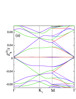
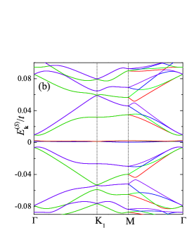
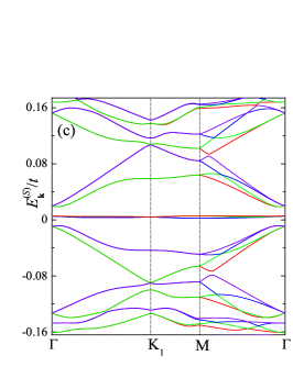
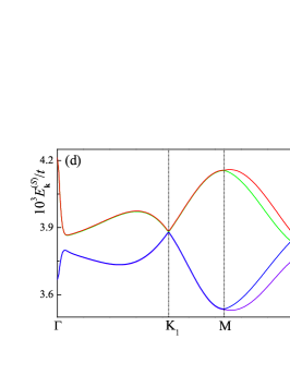
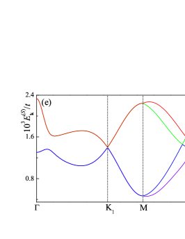
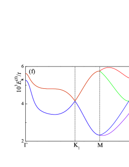
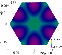
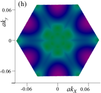
Figure 2: (a) – (c) Energy spectra for $\theta=\theta_{c}$ calculated for parametrization I (a), II.A (b), and II.B (c). The energy window for panel (c) (parametrization II.B) is about two times larger than that for panels (a) and (b). (d) – (f) Fine structures of the flat bands corresponding to panels (a) – (c), respectively. (g) – (j) Four flat low-energy bands calculated inside RBZ for parametrization II.A. The color bar is the same for all four plots [see panel (g)].

III.1 Hopping amplitude parametrization schemes

Let us consider first the single-particle properties of MAtBLG. If we neglect interactions, the electronic spectrum of the system is obtained by diagonalization of the first term of the Hamiltonian (12). The result depends on the parametrization of the hopping amplitudes $t(\mathbf{r}_{\mathbf{n}}^{is};\mathbf{r}_{\mathbf{m}}^{jr})$. In this paper we keep only nearest-neighbor terms for the intralayer hopping. The corresponding amplitude is $t=-2.57$ eV.

Unlike the intralayer hopping, there is no universally accepted parametrization scheme for the interlayer hopping amplitudes. They are much weaker than the intralayer amplitude $t$, and may be significantly affected by numerous non-universal poorly controlled factors (elastic deformations, relative layer sliding, disorder). To address this uncertainty, we will study the model (12) with three different parametrizations for the function $t(\mathbf{r};\mathbf{r}^{\prime})$. These parametrizations, as well as the single-electron spectra corresponding to them, are presented below.

The parametrization I is rather simple. The function $t(\mathbf{r};\mathbf{r}^{\prime})$ is described by the following Slater-Koster Slater and Koster (1954) formula for $p_{z}$ electrons (the corresponding contribution from $V_{\pi}(\mathbf{r})$ is assumed to be negligible):

$$t(\mathbf{r};\mathbf{r}^{\prime})=\frac{\left[(\mathbf{r}-\mathbf{r}^{\prime})\mathbf{e}_{z}\right]^{2}}{|\mathbf{r}-\mathbf{r}^{\prime}|^{2}}V_{\sigma}(\mathbf{r}-\mathbf{r}^{\prime})\,,$$ (13)

where

$$V_{\sigma}(\mathbf{r})=t_{0}e^{-(|\mathbf{r}|-d)/r_{0}}F_{c}(|\mathbf{r}|)\,,\;\;F_{c}(r)=\frac{1}{1+e^{(r-r_{c})/l_{c}}}\,.$$ (14)

The cutoff function $F_{c}(r)$ is introduced to nullify the hopping amplitudes at distances larger than $r_{c}$; we use $r_{c}=4.92$ Å, $l_{c}=0.2$ Å. The parameter $t_{0}$ defines the largest interlayer hopping amplitude. We choose $t_{0}=0.37$ eV (this value was used to describe the AB bilayer graphene Rozhkov et al. (2016)). The parameter $r_{0}$ describes how fast the hopping amplitudes decay inside the region $r<r_{c}$. We choose $r_{0}=0.34$ Å.

The parametrization I, expressed by Eqs. (13) – (14), both with and without a cutoff function, is widely used in the literature. Trambly de Laissardière et al. (2010, 2012); Suárez Morell et al. (2010, 2011); Sboychakov et al. (2019) However, in the limiting case of AB bilayer ($\theta=0$), Eqs. (13) – (14) cannot correctly reproduce the Slonczewski-Weiss-McClure (SWMc) parametrization. Indeed, the AB bilayer has three distinct nearest-neighbor interlayer hopping amplitudes: $t_{0}$ (hopping from site $1{\cal A}$ to the nearest site $2{\cal B}$), $\gamma_{3}$ (hopping from $1{\cal B}$ to $2{\cal A}$), and $\gamma_{4}$ (hopping from $1{\cal A}$ to $2{\cal A}$ and from $1{\cal B}$ to $2{\cal B}$). The parametrization I gives $\gamma_{3}=\gamma_{4}$, while experiment shows Zhang et al. (2008); Kuzmenko et al. (2009) that $\gamma_{3}>\gamma_{4}$.

To comply with the SWMc scheme, we consider yet other parametrization, designated below as ‘parametrization II’. It is a more sophisticated approach, initially proposed in Ref. Tang et al., 1996. Parametrization II takes into account the environment dependence of the hopping. That is, the electron hopping amplitude connecting two atoms at positions $\mathbf{r}$ and $\mathbf{r}^{\prime}$ depends not only on the difference $\mathbf{r}-\mathbf{r}^{\prime}$, but also on positions of other atoms in the lattice. Extra flexibility of the formalism becomes useful when the tunneling between $\mathbf{r}$ and $\mathbf{r}^{\prime}$ is depleted by nearby atoms, which act as obstacles to a tunneling electron. For tBLG, the parametrization II was used in Refs. Shallcross et al., 2010; Sboychakov et al., 2015; Rozhkov et al., 2017a, among other papers.

To use parametrization II for MAtBLG, values of several fitting parameters have to be assigned. We choose them in such a way as to correctly describe the case of the AB bilayer, with $\gamma_{3}>\gamma_{4}$ (details can be found in our previous paper Ref. Sboychakov et al., 2015). One of the fitting parameters is $t_{0}$: the largest interlayer hopping amplitude. It also scales all other interlayer hopping amplitudes. We perform all calculations for two versions of parametrization II denoted below as II.A and II.B. They have different values of $t_{0}$. All other fitting parameters are identical for II.A and II.B. Specifically, for the parametrization II.A we assign $t_{0}=0.21$ eV to guarantee that the angle $\theta_{c}$ is the same for both II.A and I (the precise definition of $\theta_{c}$ will be given below, in the next subsection). For parametrization II.B the value of $t_{0}$ is the same as for parametrization I: $t_{0}=0.37$ eV. In other words, the overall interlayer tunneling energy scale is the same for both I and II.B. However, the values of $\theta_{c}$ for these parametrizations deviate significantly from each other.

	$t_{0}$	$\theta_{c}$	$W$	$\Delta_{u}$	$\Delta_{d}$
Par. I	$0.37$ eV	$1.08^{\circ}$	$1.8$ meV	$2.7$ meV	$2.3$ meV
Par. II.A	$0.21$ eV	$1.08^{\circ}$	$4.8$ meV	$17.5$ meV	$15.5$ meV
Par. II.B	$0.37$ eV	$1.89^{\circ}$	$9.4$ meV	$33.2$ meV	$27.1$ meV

Table 1: Various single-electron characteristics of the MAtBLG spectrum for three parametrizations of the interlayer hopping.

III.2 Single-particle spectrum of MAtBLG

Once a specific parametrization is chosen, the single-electron part of our model may be diagonalized, and its single-electron spectrum may be found. Regardless of the type of the parametrization, the tBLG spectrum has common features. For each superstructure $(m_{0},\,r)$, the tBLG spectrum consists of $4N_{\text{\rm sc}}$ energy bands $E_{0\mathbf{k}}^{(S)}$ with quasimomentum $\mathbf{k}$ lying inside the reduced Brillouin zone, and $1\leq S\leq 4N_{\text{\rm sc}}$. For given $\mathbf{k}$,the energies $E_{0\mathbf{k}}^{(S)}$ are arranged in ascending order.

When the twist angle is not too small, the spectrum at low energies consists of two doubly degenerate Dirac cones located near the RBZ Dirac points $\mathbf{K}_{1}$ and $\mathbf{K}_{2}$. These Dirac cones intersect at energies above and below the cone apex energy giving rise to the low-energy van Hove singularities.

The interlayer hybridization renormalizes the Fermi velocity of the Dirac cones, making it smaller than the Fermi velocity of the single-layer graphene. At not-too-small $\theta$, the renormalized velocity decreases when $\theta$ decreases Lopes dos Santos et al. (2012); Bistritzer and MacDonald (2011). The energies of the van Hove singularities demonstrate a similar dependence on $\theta$.

The Dirac cones inherited from two graphene sheets are hosted by four bands $E_{0\mathbf{k}}^{({\cal S})}$, with ${\cal S}=2N_{\text{\rm sc}}-1,\,2N_{\text{\rm sc}},\,2N_{\text{\rm sc}}+1,\,2N_{\text{\rm sc}}+2$. Since in a pristine or weakly doped sample these are the single-electron states closest to the Fermi energy, the low-temperature properties of the MAtBLG are controlled by these bands. Consequently, their total width $W$ defined as

$$W=\max_{\mathbf{k}}(E_{0\mathbf{k}}^{(2N_{\text{\rm sc}}+2)})-\min_{\mathbf{k}}(E_{0\mathbf{k}}^{(2N_{\text{\rm sc}}-1)})$$ (15)

is an important characteristics of the MAtBLG spectrum. As long as the twist angle is not too small, $W$ decreases with decreasing $\theta$.

Both numerical and analytical studies demonstrate that both the Fermi velocity and the width $W$ experience substantial reduction as $\theta_{c}$ decreases. Yet, in a wide range of $\theta$, the tBLG formally remains a semimetal at the charge neutrality point. However, at some critical twist angle $\theta_{c}$ the system acquires a Fermi surface even at zero doping. For $\theta<\theta_{c}$ the tBLG remains in a formally metallic state.

The value of $\theta_{c}$ is not universal, and depends on particulars of the interlayer tunneling. For parametrizations I and II.A one has $\theta_{c}\cong 1.08^{\circ}$ [$(m_{0},\,r)=(30,\,1)$]. For parametrization II.B, the Fermi surface arises at larger angle, $\theta_{c}\cong 1.89^{\circ}$ [$(m_{0},\,r)=(17,\,1)$]. With further decrease of the twist angle, the bandwidth $W$ becomes an oscillating function of $\theta$. For all three parametrizations under study, the width $W$ has a minimum at $\theta=\theta_{c}$. For each parametrization, the numerical calculations presented below were performed at $\theta=\theta_{c}$ (one must remember that $\theta_{c}$ is a parametrization-specific quantity).

Formally speaking, our $\theta_{c}$ differs from the common definition of the first magic angle introduced in Ref. Bistritzer and MacDonald, 2011. According to the latter, the first magic angle corresponds to nullification of the Fermi velocity at the Dirac points, yet, in our study this velocity remains non-zero when $\theta=\theta_{c}$. While both definitions give similar values of the twist angle, these values are not identical. We choose to work in the regime of smallest $W$ since the logic of the mean-field approximation suggests that this regime corresponds to the largest condensation energy.

The low-energy structure of the numerically calculated spectra at $\theta=\theta_{c}$, are shown in Figs. 2(a) – (c) for all three parametrizations. The finer details for the flat bands $E_{0\mathbf{k}}^{({\cal S})}$ may be examined in Figs. 2(d) – (f). We show the bands along the contour ${\bm{\Gamma}}\to\mathbf{K}_{1}\to\mathbf{M}\to{\bm{\Gamma}}$. Qualitatively, the low-energy spectra for all parametrizations look very similar. We see a Dirac cone near point $\mathbf{K}_{1}$, local extrema near the $\mathbf{M}$ point, and complicated behavior on the line $\mathbf{M}\to{\bm{\Gamma}}$.

On the quantitative level, however, the characteristics of the low-energy bands are different. For example, the bandwidth $W$ for the parametrization II.B is about $6$ times larger than that for the parametrization I, and about $2$ larger than that for the parametrization II.A. Other important parametrization-dependent quantities are the energy gaps separating the flat bands $E_{0\mathbf{k}}^{({\cal S})}$ from dispersive bands at higher and lower energies. Formally speaking, these gaps can be defined as

$$\Delta_{d} = \max_{\mathbf{k}}(E_{0\mathbf{k}}^{(2N_{\text{\rm sc}}-2)})-\min_{\mathbf{k}}(E_{0\mathbf{k}}^{(2N_{\text{\rm sc}}-1)}),$$

$$\Delta_{u} = \max_{\mathbf{k}}(E_{0\mathbf{k}}^{(2N_{\text{\rm sc}}+2)})-\min_{\mathbf{k}}(E_{0\mathbf{k}}^{(2N_{\text{\rm sc}}+3)}).$$ (16)

Our numerical data demonstrates that the values of $\Delta_{u}$ and $\Delta_{d}$ for parametrizations II.A and II.B exceed the values for the parametrization I by order of magnitude. The characteristics of the low-energy spectra for all three parametrizations at $\theta=\theta_{c}$ are summarized in Table 1.

Finally, let us briefly discuss the symmetry properties of the flat bands. Figures 2(g) – (j) show the low-energy spectra calculated inside the reduced Brillouin zone for parametrization II.A. We see that the spectra have hexagonal symmetry. Spectra are also symmetric under reflections with respect to the axes parallel and perpendicular to $\mathbf{G}_{1}$, $\mathbf{G}_{2}$, and $\mathbf{G}_{1}+\mathbf{G}_{2}$. All these symmetries are observed also for the other parametrizations as well. However, below we will see that the symmetry of the low-energy spectra can be reduced if we include interactions into account.

III.3 Structure of the SDW order parameters

The system having flat bands intersecting the Fermi level is very susceptible to interactions. In our model, the interactions are described by the second and the third terms in the total Hamiltonian (12). They represent the on-site and intersite Coulomb repulsion. Interactions spontaneously break symmetries of the single-particle Hamiltonian generating a finite order parameter. We assume here that this order parameter is a spin density wave. This choice is not arbitrary. It was shown in many papers (see, e.g., Refs. Lopes dos Santos et al., 2012; San-Jose et al., 2012; Sboychakov et al., 2015), that at small twist angles, electrons at the Fermi level occupy mainly the regions with almost perfect AA stacking within a supercell. At the same time, it was demonstrated theoretically Rakhmanov et al. (2012); Sboychakov et al. (2013a, b); Akzyanov et al. (2014) that the ground state of the AA stacked bilayer graphene should be antiferromagnetic. For this reason we believe that the SDW should be a good candidate for the ground state of the MAtBLG.

Our SDW order parameter is a multicomponent one. First, it contains terms proportional to the on-site expectation values of electrons with opposite spins. To be more specific, we define

$$\Delta_{\mathbf{n}is}=U\langle d^{{\dagger}}_{\mathbf{n}is\uparrow}d^{\phantom{{\dagger}}}_{\mathbf{n}is\downarrow}\rangle\,.$$ (17)

These components are controlled by the Hubbard interaction. We take $U=2t$. This value is somewhat smaller than the critical value for a single-layer graphene transition into a mean-field antiferromagnetic state Sorella and Tosatti (1992), $U_{c}=2.23t$. Thus, our Hubbard interaction is rather strong, but not too strong to open a gap in the single layer graphene.

Next, we include the intralayer nearest-neighbor SDW order parameter. In a graphene layer, each atom in one sublattice has three nearest-neighbors belonging to another sublattice (for example, an atom on sublattice ${\cal B}$ has three nearest neighbors on sublattice ${\cal A}$). For this reason we consider three types of intralayer nearest-neighbor order parameters, $A^{(\ell)}_{\mathbf{n}i\sigma}$ ($\ell=1,\,2,\,3$), corresponding to three different links connecting the nearest-neighbor sites. These order parameters are defined as follows

$$A^{(\ell)}_{\mathbf{n}i\sigma}=V_{\rm nn}\langle d^{{\dagger}}_{\mathbf{n}+\mathbf{n}_{\ell}i{\cal A}\sigma}d^{\phantom{{\dagger}}}_{\mathbf{n}i{\cal B}\bar{\sigma}}\rangle\,,$$ (18)

where $\mathbf{n}_{1}=(0,\,0)$, $\mathbf{n}_{2}=(1,\,0)$, $\mathbf{n}_{3}=(0,\,1)$, $\bar{\sigma}=-\sigma$, and $V_{\rm nn}=V(|\bm{\delta}|)$ is the in-plane nearest-neighbor Coulomb repulsion energy. We take $V_{\text{nn}}/U=0.59$, in agreement with Ref. Wehling et al., 2011.

Finally, we consider the interlayer SDW order parameter. It is defined as follows

$$B^{rs}_{\mathbf{m};\mathbf{n}\sigma}=V(\mathbf{r}^{1r}_{\mathbf{m}}-\mathbf{r}^{2s}_{\mathbf{n}})\langle d^{{\dagger}}_{\mathbf{m}1r\sigma}d^{\phantom{{\dagger}}}_{\mathbf{n}2s\bar{\sigma}}\rangle\,.$$ (19)

For calculations we assume that $B^{rs}_{\mathbf{m};\mathbf{n}\sigma}$ is non-zero only when sites $\mathbf{r}_{\mathbf{m}}^{1s}$ and $\mathbf{r}_{\mathbf{n}}^{2r}$ are sufficiently close. Namely, if the hopping amplitude connecting $\mathbf{r}_{\mathbf{m}}^{1s}$ and $\mathbf{r}_{\mathbf{n}}^{2r}$ vanishes, then the parameter $B^{rs}_{\mathbf{m};\mathbf{n}\sigma}$ is zero. The number of non-zero $B^{rs}_{\mathbf{m};\mathbf{n}\sigma}$ depends on the type of the hopping amplitude parametrization. For parametrizations II.A and II.B we have up to three non-zero $B^{rs}_{\mathbf{m};\mathbf{n}\sigma}$ for a given $\mathbf{n}$, $r$, $s$, and $\sigma$. For parametrization I we have up to $9$ such $B^{rs}_{\mathbf{m};\mathbf{n}\sigma}$. Assuming screening is small at short distances we model the function $V(\mathbf{r})$ in Eq. (19) as $V(\mathbf{r})\propto 1/|\mathbf{r}|$ with $V(d)=V_{\text{nn}}|\bm{\delta}|/d=0.25U$.

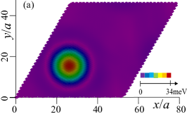
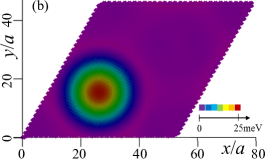
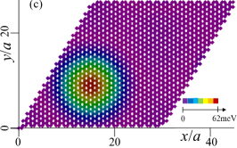
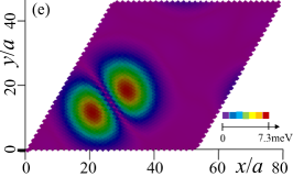
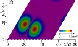
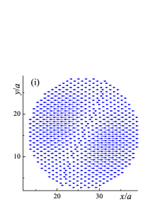
Figure 3: Characteristics of the SDW order at the charge neutrality point. (a) – (c) Spatial distributions of the absolute values of the on-site order parameter $\Delta_{\mathbf{n}1s}$ in layer $1$, Eq. (17), within a single supercell [the supercell position relative to the MAtBLG lattice is the same as in Fig. 1 (a)]. The order parameter is calculated for parametrizations I (a), II.A (b), and II.B (c). Since different parametrizations have different values of $\theta_{c}$, the superlattice cell area for parametrization II.B is about four times smaller than that for parametrizations I and II.A. (d) – (f) Spatial distributions of the in-plane (layer 1) order parameter $\mathfrak{A}^{(\ell)}_{\mathbf{n}1}=|A^{(\ell)}_{\mathbf{n}1\uparrow}+A^{(\ell)*}_{\mathbf{n}1\downarrow}|$ for $\ell=1$ (d), $\ell=2$ (e), and $\ell=3$ (f), calculated for parametrization I. (g) – (i) Spins on the links, Eq. (IV.1), corresponding to order parameters $A^{(\ell)}_{\mathbf{n}i\sigma}$ with $\ell=1$ (g), $\ell=2$ (h), and $\ell=3$ (i), calculated for parametrization I. Only the AA region of the superlattice cell is shown.

We assume superlattice periodicity for all three types of SDW order parameters. A superlattice translation preserves the SDW texture. With this constraint we write down the system of mean-field equations for the functions $\Delta_{\mathbf{n}is}$, $A^{(\ell)}_{\mathbf{n}i\sigma}$, and $B^{rs}_{\mathbf{m};\mathbf{n}\sigma}$, and solve it numerically for different doping levels, $n$, varying from $-4$ to $+4$ extra electrons per supercell. Details of the calculation procedure are given in the Appendix.

III.4 Approximation quality

There are several circumstances which we must keep in mind assessing the reliability of the approximations utilized in this study. Our approach is based on the mean-field framework. It is well-known that the mean-field approximation is reliable for: (i) a three-dimensional model; (ii) in the limit of weak coupling; (iii) with a single order parameter. If either of these three conditions is violated, more care is necessary interpreting the obtained results.

As our system is two-dimensional, finite-temperature long-range order in the MAtBLG is impossible, as postulated by the Hohenberg-Mermin-Wagner theorem. Yet, it is believed that, despite the absence of the true order, the mean-field energy scale remains an observable quantity: it may be experimentally measured as a low-$T$ single-particle (pseudo)gap. Consistent with this expectation, our calculations reproduce energy scales observed in experiment, see the Discussion for details.

Further, many real-life systems violate condition (ii). To address this issue for the MAtBLG, let us evaluate the effective coupling constant for our model using the following argument. The main contribution to the formation of SDW order comes from the flat bands. Thus, the effective Hubbard interaction can be estimated as

$$U_{\rm eff}=U\sum_{n}|\Phi_{n}|^{4},$$

where $\Phi_{n}$ is the wave function of the flat band in real space representation, and the summation is performed over all sites within a single supercell. Since the electrons at the Fermi level are localized inside the AA region of the superlattice, occupying about 1/3 of the superlattice’s area, one can write that inside this region

$$|\Phi_{n}|\sim\sqrt{3/N_{\rm sc}},$$

and we obtain the estimate

$$U_{\rm eff}\sim 3U/N_{\rm sc}.$$

Substituting specific numbers, we obtain $U_{\rm eff}=5.5$ meV for parametrizations I and II.A, and $U_{\rm eff}=16.8$ meV for parametrizations II.B. These values must be compared against the width of the flat bands $W$, see Table 1. Since $U_{\rm eff}/W$ for all parametrizations is of the order of unity, the studied model is in the limit of intermediate coupling. As the ratio $U_{\rm eff}/W$ grows beyond unity, the mean-field approximation becomes progressively less controlled, but we expect that our results remain qualitatively valid at not too strong interaction. As an example of a successful application of the mean-field calculations in the intermediate-coupling regime see Ref. Zaanen and Gunnarsson, 1989.

Another complication would be the violation of the condition (iii) above: for the MAtBLG, several (metastable) order parameters compete against each other to become the true ground state. This situation is not unique, and similar competitions were discussed in the contexts of other models Rozhkov (2009); Sboychakov et al. (2013c); Igoshev et al. (2010); Rozhkov et al. (2017b). Since there is no known procedure which allows one to compile an exhaustive list of metastable phases for a given Hamiltonian, a compromise based on general physical arguments, input from experiments, and other factors is unavoidable. It is not surprising, therefore, that our numerical search for the most optimal order parameter is constrained in several respects. We already pointed out that the order parameters violating superlattice translations are not considered as they incur unacceptable computational costs.

Also, the numerical implementation of our mean-field procedure does not account for non-coplanar spin textures, whose relevance for the studied system is an open question. Non-coplanar textures naturally appear Lu et al. (2020) in recently introduced effective models Lu et al. (2020); Liu et al. (2018); Isobe et al. (2018); You and Vishwanath (2019), where they stabilize due to Fermi surface nesting and a significantly enhanced symmetry group. To which extent the weak-coupling nesting-based argument of Refs. Lu et al., 2020; Liu et al., 2018; Isobe et al., 2018 is applicable to the MAtBLG (a system in intermediate-coupling regime You and Vishwanath (2019), with very complex Fermi surface Sboychakov et al. (2015)) remains an interesting issue for future studies.

Finally, our procedure, as it is described above, does not attempt to obtain self-consistency for the charge density distribution within a supercell. Indeed, one must remember that, since the atoms locations within a supercell are not equivalent to each other, the average charge on a given atom depends on its position (the same is true for the local density of states). In principle, the interaction attempts to suppress spatial variations of charge through “Hartree” terms; however, we neglect them in our numerical code.

IV Results: Spatial distributions of SDW order parameters.

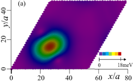
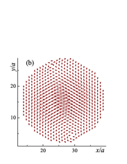
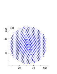
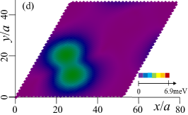
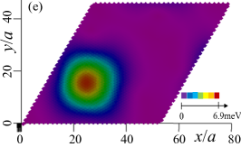
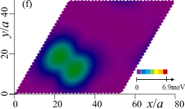
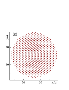
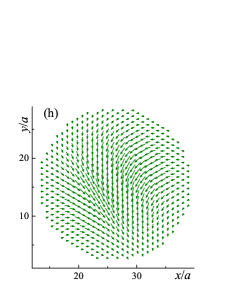
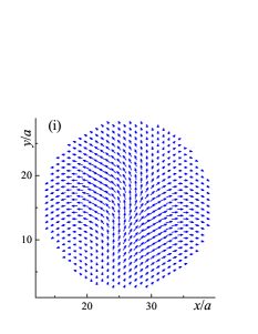
Figure 4: Characteristics of the SDW order at the half-filled state ($\nu=2$). (a) Spatial distribution of $|\Delta_{\mathbf{n}1s}|$ within a single supercell [the supercell position relative to the MAtBLG lattice is the same as in Fig. 1 (a)]. (b) – (c) Orientations of the on-site spins, Eq. (20), in the layer 1, sublattice ${\cal A}$ (b) and ${\cal B}$ (c) shown inside the AA region of the supercell. (d) – (f) Spatial distributions of $\mathfrak{A}^{(\ell)}_{\mathbf{n}1}=|A^{(\ell)}_{\mathbf{n}1\uparrow}+A^{(\ell)*}_{\mathbf{n}1\downarrow}|$ within a single supercell, for $\ell=1$ (d), $\ell=2$ (e), and $\ell=3$ (f). (g) – (i) Spins on the links corresponding to the order parameters $A^{(\ell)}_{\mathbf{n}i\sigma}$, with $\ell=1$ (g), $\ell=2$ (h), and $\ell=3$ (i), shown inside the AA region of the superlattice cell. The order parameters shown are calculated for parametrization I. Similar pictures are obtained for parametrizations II.A and II.B.

In this section we present the results of our calculation of the SDW order parameters and analyze their symmetry properties. The spatial distribution of the order parameters inside the superlattice cell is different for different doping levels. However, it turns out that for a given doping the properties of the order parameters are very similar for the three parametrizations used.

IV.1 Charge neutrality point

We start from the charge neutrality point. Figures 3(a) – (c) show the color plots of the spatial distribution of the absolute values of the on-site order parameter in layer 1, $|\Delta_{\mathbf{n}1s}|$, calculated for three parametrizations. Similar structures are observed for layer 2. We see that the maximum values of the $\Delta_{\mathbf{n}1s}$ are different for the three parametrizations, but the plots themselves look very similar. The maxima of $\Delta_{\mathbf{n}1s}$ are located in the center of the AA region of the superlattice cell [c.f. with Fig. 1(a)]. The order parameter $\Delta_{\mathbf{n}is}$ defines the spin on a site in position $\mathbf{n}$, layer $i$, and sublattice $s$, as follows:

$$\mathbf{S}_{\mathbf{n}is}=\frac{1}{U}\left(\operatorname{Re}\Delta_{\mathbf{n}is},\,\operatorname{Im}\Delta_{\mathbf{n}is},\,0\right).$$ (20)

A vanishing $z$ component of $\mathbf{S}_{\mathbf{n}is}$ in our definition (20) implies that only planar spin textures are allowed (this is a limitation of our numerical code, as explained in Sec. III.4). However, at the charge neutrality point this constraint turns out to be unimportant, since all spins are collinear. If in layer 1 and sublattice ${\cal A}$ (and in layer 2 and sublattice ${\cal B}$) they point in one direction (along the $x$ axis), then the layer 1 and sublattice ${\cal B}$ (and in layer 2 and sublattice ${\cal A}$) they point in the opposite direction. Thus, we have antiferromagnetic ordering of spins.

Let us now visualize the intralayer nearest-neighbor order parameters $A^{(\ell)}_{\mathbf{n}1\sigma}$. Using these quantities one can define the spins on the link connecting nearest-neighbor sites in each layer as follows:

$$\mathbf{S}^{(\ell)}_{\mathbf{n}i} \!\equiv\! \frac{1}{2}\sum_{\sigma\sigma^{\prime}}\!\bm{\sigma}_{\sigma\sigma^{\prime}}\langle d^{{\dagger}}_{\mathbf{n}+\mathbf{n}_{\ell}i{\cal A}\sigma}d^{\phantom{{\dagger}}}_{\mathbf{n}i{\cal B}\sigma^{\prime}}\rangle+{\rm c.c.}$$

$$\!=\! \frac{1}{V_{\text{nn}}}\!\left(\operatorname{Re}[A^{(\ell)}_{\mathbf{n}i\uparrow}+A^{(\ell)}_{\mathbf{n}i\downarrow}],\,\operatorname{Im}[A^{(\ell)}_{\mathbf{n}i\uparrow}-A^{(\ell)}_{\mathbf{n}i\downarrow}],\,0\right),$$

where $\bm{\sigma}$ is a three-component vector composed of the Pauli matrices. The quantity

$$\mathfrak{A}^{(\ell)}_{\mathbf{n}1}=|A^{(\ell)}_{\mathbf{n}1\uparrow}+A^{(\ell)*}_{\mathbf{n}1\downarrow}|$$

is proportional to the absolute values of $\mathbf{S}^{(\ell)}_{\mathbf{n}i}$ calculated in layer 1 for parametrization I. The spatial distributions of $\mathfrak{A}^{(\ell)}_{\mathbf{n}1}$ are shown in Figs. 3(d) – (f) for all three possible values of $\ell$. The distributions are shaped like dumbbells localized in the AA region of the superlattice. The orientations of these dumbbells are different for different orientations of the carbon-carbon links. Similar figures are obtained for other two parametrizations. The directions of the vectors $\mathbf{S}^{(\ell)}_{\mathbf{n}i}$ inside the AA region are shown in Figs. 3(g) – (i). We see that all spins $\mathbf{S}^{(\ell)}_{\mathbf{n}i}$ are collinear; but if in one part of a dumbbell they point in one direction, then in another part of the dumbbell they are oriented in the opposite direction.

Absolute values of the order parameters $A^{(\ell)}_{\mathbf{n}i\sigma}$ are several times smaller than that for $\Delta_{\mathbf{n}is}$. Our calculations show that the interlayer order parameters $B^{rs}_{\mathbf{m};\mathbf{n}\sigma}$ are one order of magnitude smaller than $A^{(\ell)}_{\mathbf{n}i\sigma}$; thus, we do not discuss them here in details.

We now demonstrate that the calculated SDW magnetization texture has the same geometrical symmetries as the tBLG superstructure. We start with the following observation about the tBLG lattice symmetry. The center of the AA region of the superlattice cell is located at $\mathbf{R}_{\text{AA}}=(\mathbf{R}_{1}+\mathbf{R}_{2})/3$. For the $r=1$ superstructures considered here, one can prove using Eqs. (2), (4), and (5) that

$$\mathbf{R}_{\text{AA}}=m_{0}\mathbf{a}_{2}-\mathbf{a}_{1}+2\bm{\delta}=m_{0}\mathbf{a}^{\prime}_{2}+\bm{\delta}^{\prime}\,.$$ (22)

It is easily seen from this equation that the point $\mathbf{R}_{\text{AA}}$ is located at the center of the hexagons of both layers. This means that the tBLG lattice is invariant under a rotation by $60^{\circ}$ around the axis perpendicular to the layers and passing through the point $\mathbf{R}_{\text{AA}}$.

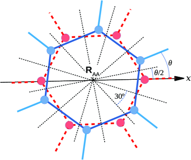
Figure 5: Mirror symmetries of the tBLG. Point $\mathbf{R}_{\text{AA}}=(\mathbf{R}_{1}+\mathbf{R}_{2})/3$ is the center of the AA region of the superlattice cell. The solid (blue) lines represent carbon-carbon bonds in the (rotated) top layer, dashed (red) lines correspond to the bonds in the (immobile) bottom layer. The circles represent carbon atoms. Thin dashed (black) lines are the reflection axes. It is easy to see from this figure that a reflection relative to any of these axes, accompanied by exchange of the layers, leaves the tBLG lattice unchanged.

Further, the tBLG lattice also has mirror-like symmetries. Indeed, the lattice remains invariant if one exchanges layers and then performs a reflection with respect to a certain axis in the $xy$-plane passing through point $\mathbf{R}_{\text{AA}}$, see Fig. 5. There are six such axes. They cross the $x$-axis at $30^{\circ}p+\theta/2$, where $p=0,1,\ldots,5$. Since for the superstructures considered the twist angle is small, any mirror symmetry axis is either approximately parallel to $\mathbf{R}_{1}$, $\mathbf{R}_{2}$, or $(\mathbf{R}_{1}-\mathbf{R}_{2})$, or approximately perpendicular to one of these vectors.

One can easily see from Figs. 3(a) – (f) that the SDW order parameters are invariant with respect to all geometrical symmetries of the tBLG lattice. Indeed, the on-site order parameter does not change under the action of the rotations and reflections mentioned above, while the intersite order parameters $\mathfrak{A}^{(\ell)}_{\mathbf{n}i}$ either remain invariant or convert into $\mathfrak{A}^{(\ell^{\prime})}_{\mathbf{n}i}$, with $\ell^{\prime}\neq\ell$.

IV.2 Half-filled state

Our simulations show that doping of the system away from the charge-neutrality point spontaneously reduces the symmetry of the SDW order parameters. For illustration of this fact we consider only the case of half-filling, which corresponds to $2$ extra electrons or extra holes per supercell. Electron and hole dopings are equivalent at the qualitative level; thus, for definiteness, we consider electron doping. Figure 4(a) shows the spatial distribution of $|\Delta_{\mathbf{n}1s}|$, calculated for parametrization I. A similar pattern is observed in layer $2$. We see that in contrast to Fig. 3(a) the spatial profile becomes uniaxially stretched. The stretching axis is (approximately) parallel to the vector $(\mathbf{R}_{1}+\mathbf{R}_{2})$. As a result of this distortion, the $60^{\circ}$ rotation is no longer a symmetry of the system. However, the spatial profile is still symmetric under $180^{\circ}$ rotation around ${\bf R}_{\rm AA}$. Regarding the mirror symmetry, only axes parallel and perpendicular to $(\mathbf{R}_{1}-\mathbf{R}_{2})$ remain mirror symmetry axes. Another difference, in comparison to the charge-neutrality point, is that the on-site spins are no longer collinear, even though an antiferromagnetic type configuration is preserved, see Figs. 4(b) – (c).

The change in the inter-site order parameters under doping is even more dramatic: the spatial profile for $\mathfrak{A}^{(\ell)}_{\mathbf{n}1}$ with $\ell=2$ does not have the form of a dumbbell, Fig. 4(e), and it is different from that for $\ell=1$ and $\ell=3$, Figs. 4(d), (f). However, the $180^{\circ}$ rotation symmetry endures for all three types of intersite order parameters. Moreover, the symmetry under the reflection with respect to the axis parallel to $(\mathbf{R}_{1}-\mathbf{R}_{2})$ also remains unbroken. This reflection transforms the profiles shown in Figs. 4(e), (f) into each other, while the profile of Fig. 4(d) is unchanged. Likewise, one can argue that the line perpendicular to $(\mathbf{R}_{1}-\mathbf{R}_{2})$ is also a valid symmetry axis for the inter-site texture. Finally, our calculations demonstrate that vectors $\mathbf{S}^{(\ell)}_{\mathbf{n}1}$ are no longer collinear, and their textures have a complicated structure.

Thus, at half-filling the symmetry of the order parameters is partially reduced, indicating spontaneous formation of the electron nematic state. The nematicity of the ordered state in doped MAtBLG is a robust property which does not require fine-tuning. Indeed, the rotation symmetry of the order parameter is lowered for all three parametrizations studied in this paper.

The nematicity also manifests itself in the local DOS, see Fig. 6. The two panels of this figure show the local DOS at the Fermi energy for the half-filled ($\nu=2$) and $\nu=2.25$ states. In both cases, the local density of states demonstrates invariance under the $C_{2}$ point symmetry group, which is smaller than $C_{6}$ of the MAtBLG moiré superlattice. In this context, the symmetry reduction can be interpreted as a type of commensurate charge-density wave, with the modulation wave vector ${\bf Q}_{\rm cdw}$ being equal to zero in the RBZ. In real space the charge modulation has the same period as the superlattice. To discriminate between the superlattice and the charge-density wave in experiments, one has to rely on differences in the point symmetry groups of the two.

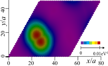
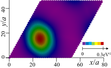
Figure 6: Local density of states at the Fermi energy for the many-body states with nematicity. Both panels present a single supercell, whose position relative to the MAtBLG lattice is the same as in Fig. 1 (a). The numerical data in the top panel is for $\nu=2$ (half filling, two extra electrons per supercell), in the bottom panel is for $\nu=2.25$. For both filling fractions, the local densities of states demonstrate a $C_{2}$ point symmetry group, instead of the larger $C_{6}$ group of the moiré superlattice. This manifestation of nematicity may be detected in STM experiments.

V Results: The low-energy band structure

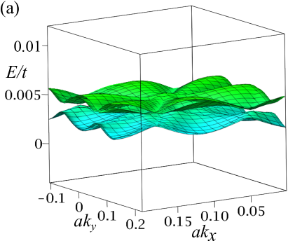
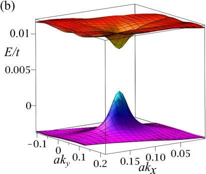
Figure 7: The spectrum of the non-interacting model (a) compared with the spectrum calculated within the mean-field approximation (b). The spectrum in (a) consists of four warped bands, each band is spin-degenerate. In (b), two quartets of single-electron bands are visible, while the individual bands are indiscernible on this scale. We see that the characteristic gap-inducing splitting between the quartets exceeds the warping of the non-interacting single-electron bands. The calculations were performed at the charge neutrality point $n=0$, for parametrization II.B.

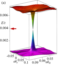
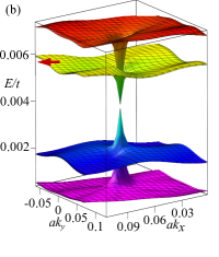
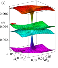
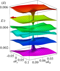
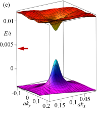
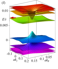
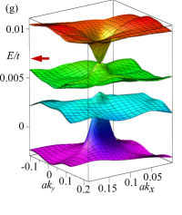
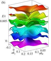
Figure 8: Mean-field low-energy spectra calculated at different integer-valued doping levels for parametrizations I [(a) – (d)] and II.B [(e) – (h)]. Doping levels are: $\nu=0$ [(a), (e)], $\nu=1$ [(b), (f)], $\nu=2$ [(c), (g)], and $\nu=3$ [(d), (h)]. The red thick arrow near the $E/t$ axis marks the position of the Fermi level.

V.1 Symmetry of the mean-field low-energy spectra

If interactions are neglected, the tBLG single-electron states are doubly degenerate. The SDW order parameters lift the spin degeneracy. As a result, at low energies we have eight non-degenerate flat bands. Figure 7 allows one to compare the spectrum of the non-interacting model with the mean-field spectrum at the charge neutrality point. The degeneracy-lifting patterns for different doping levels and parametrizations are illustrated by plots in Figs. 8(a) – (h) which show the low-energy spectra inside a reciprocal supercell (this data will be discussed in detail in subsection V.2, see also Ref. Sboychakov et al., 2019).

However, the lifting of the spin degeneracy is not the only consequence of the SDW ordering. The geometrical symmetries of the order parameter affect the symmetries of the single-electron mean-field spectrum as well. The plots in Figs. 8 are not convenient for discussion of this issue, and we will use Figs. 9(a) – (d), which present individual color plots of the mean-field bands calculated at different doping levels inside the RBZ [similar data for the non-interacting case is shown in Figs. 2(g) – (j)], instead.

We start from the charge neutrality point. At zero doping, the low-energy bands bundle into two groups (four bands per group) of nearly degenerate bands, see Figs. 8(a,e). Such a group will be called a quartet Sboychakov et al. (2019). The separation between bands within a specific quartet is finite. However, it is much smaller than the characteristic separation between the quartets themselves. Because of this near-degeneracy, it is sufficient to choose a single band to represent a given quartet. Of four bands in each quartet, the bands closest to the Fermi level are shown in Fig. 9(a) – (b). These plots have the same symmetries as those in Figs. 2(g) – (j): they all are symmetric under rotations of $60^{\circ}$ around the $\Gamma$ point, they also have six mirror symmetry axes, parallel and perpendicular to $\mathbf{G}_{1}$, $\mathbf{G}_{2}$, and $(\mathbf{G}_{1}+\mathbf{G}_{2})$. The other bands in quartets all have the same symmetries, independent of a specific parametrization.

Doping reduces the symmetry of the SDW order parameters. As a result, the symmetry of the mean-field spectrum is also reduced. To illustrate this, in Figs. 9(c) – (d) we present color plots of two low-energy bands closest to the Fermi level (one is filled, the other is empty) calculated for parametrization II.A at doping $\nu=-2$. The spectra now do not exhibit hexagonal symmetry, but they are still symmetric under a $180^{\circ}$ rotation around the $\Gamma$ point. There are also two mirror symmetry axes, parallel and perpendicular to $(\mathbf{G}_{1}+\mathbf{G}_{2}$). Similar pictures are observed for electron doping and for the two other parametrizations.

V.2 Mean-field low-energy spectra: evolution with doping

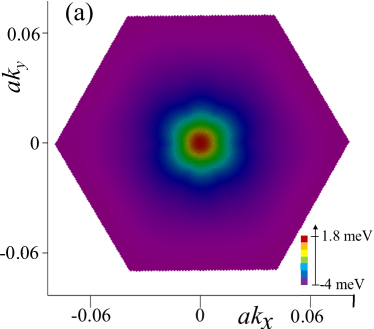
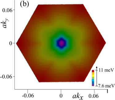
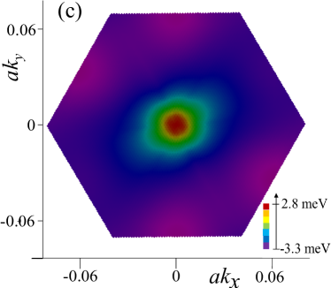
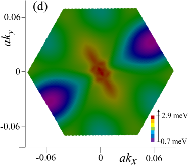
Figure 9: Color plots of the mean-field low-energy bands closest to the Fermi level calculated at the charge neutrality point [panels (a) and (b)] and at $\nu=-2$ [panels (c) and (d)]; parametrization II.A. Each plot has its individual color bar. Nematicity-induced reduction of the point symmetry group from $C_{6}$ [(a) and (b)] to $C_{2}$ [(c) and (d)] is clearly seen.

We reported previously Sboychakov et al. (2019) that the structure of the low-energy single-electron spectrum strongly depends on the doping level. The study in Ref. Sboychakov et al., 2019 was performed for a single parametrization (the parametrization employed in Ref. Sboychakov et al., 2019 is a version of parametrization I). Below we will extend that analysis by comparing spectra calculated for different parametrizations. Our main findings are summarized in Figs. 8(a) – (h). These show the spectra inside a reciprocal supercell (centered at the $\Gamma$ point) calculated for parametrizations I and II.B at four integer-valued doping levels $\nu=0,\,1,\,2\,,3$. The structures for negative doping levels $n$ are very similar to that for positive dopings $|n|$.

For fixed doping, the change of parametrization does not introduce qualitative modifications to the spectrum. However, several quantitative characteristics are sensitive to the parametrization choice.

V.2.1 Charge neutrality point

At the charge neutrality point, the eight low-energy bands split into two quartets. Except for a small vicinity of the $\Gamma$ point, the energy $\Delta_{s}$ separating the quartets is almost constant everywhere in the RBZ. The specific value of $\Delta_{s}$ depends on the parametrization: for case I one has $\Delta_{s}\approx 15$ meV. A similar value ($\Delta_{s}\approx 14$ meV) was found for parametrization II.A. At the same time, for the case II.B this quantity is significantly larger $\Delta_{s}\approx 40$ meV.

At the $\Gamma$ point, the separation between the quartets is the smallest. For parametrization I, see Fig. 8 (a), the splitting between upper and lower quartets is $\sim 9\times 10^{-5}t$. Such a splitting is smaller, but comparable to, the splitting of the non-interacting bands close to the $\Gamma$ point, as shown in Fig. 2 (d). At the $\Gamma$ point, each quartet consists of two doublets, the splitting between doublets is about $8\times 10^{-6}t$. A similar situation takes place for other two parametrizations, with the only difference being that the splitting between quartets is one order of magnitude larger than for parametrization I. Thus, on a qualitative level, the band structures at the $\Gamma$ point are similar for all three parametrizations.

The spectra of non-interacting models are four-fold degenerate [(two-fold spin degeneracy) times (two-fold valley degeneracy)] at the $\Gamma$ point [see Figs. 2 (d)-(f)]. Thus, the SDW order partially lifts this degeneracy.

V.2.2 Doped states

For $\nu=\pm 1$, each quartet splits into a group of three bands (a triplet) and a single band (a singlet), with the chemical potential in the (partial) gap between the triplet and the singlet. At half-filling ($\nu=\pm 2$) each quartet is transformed into two doublets. The chemical potential is between the doublets. When we have three extra electrons (or extra holes) per supercell, $\nu=\pm 3$, the upper (lower) quartet is separated into the doublet and two upper (lower) singlets. For electron (hole) doping, the chemical potential lies between the upper (lower) singlets.

As one can see from Fig. 8(h), for parametrization II.B at $|\nu|\approx 3$, the band warping becomes comparable to the band splitting. This effect is even more pronounced for parametrization II.A. We note that the (approximate) band degeneracy at the $\Gamma$ point persists for all parametrizations and all levels of doping.

It is instructive to interpret the doping-induced band structure reconstructions in terms of the minimization of the total energy. At the charge-neutrality point, splitting of the eight bands into two quartets acts to lower the total energy, since only four of eight bands are filled. At half-filling (two extra electrons per supercell), the single-particle energy is optimized if a filled doublet splinters away from the quartet and sinks beneath the Fermi level.

When we have only one extra electron per supercell it is favorable to separate the lower single band (filled) from the quartet. Finally, when we have three extra electrons per supercell, the three filled energy bands from the quartet separate from the upper empty one.

As a result of the spectrum reconstruction, the density of states at the Fermi energy $\rho(\varepsilon_{F})$ becomes a non-monotonic function of $n$, see Fig. 10. One observes that the density of states has a local minimum near or at the integer value of $\nu$ for all three parametrizations. At the same time, the dependence of $\rho(\varepsilon_{F})$ on $n$ is sensitive to details of the interlayer hopping. For example, the minimum at $\nu=3$ is very shallow in panel (b) of Fig. 10, it is more pronounced in panels (c), and in panel (a) the density of state drops to zero at $\nu=3$. Similar oscillations of the DOS were observed experimentally (for details see next section).

VI Discussion

We argued that doping of the system away from the charge neutrality point reduces the symmetry of both the order parameters and the electronic spectrum giving rise to the SDW-driven electronic nematic state. The SDW order parameters monotonically decrease when doping goes away from zero. On the other hand, the nematicity demonstrates a different trend. Our calculations show that for doping $|\nu|\lesssim 0.5$, the nematicity is virtually absent. At larger doping it starts growing and achieves maximum at half-filling, that is for $2$ extra electrons or holes per supercell. With further increase of doping the nematicity decays, and at $|\nu|\approx 4$ it vanishes together with the SDW order parameters.

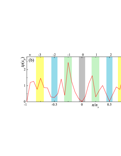
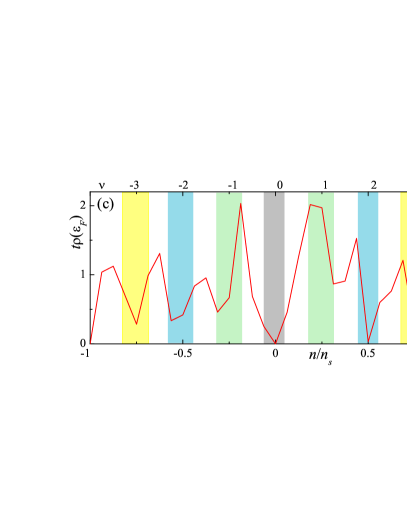
Figure 10: The density of states at the Fermi level $\rho(\varepsilon_{F})$ as a function of doping $n$, for different parametrizations: panel (a) corresponds to parametrization I, panels (b) and (c) show the results for the cases II.A and II.B. Colored rectangles mark the areas near integer values of $\nu=n/(n_{s}/4)$. For all parametrizations, the density of states has local minima near or at integer $\nu$. At the same time, finer details of $\rho(\varepsilon_{F})$ are sensitive to the particulars of the interlayer hopping. Specifically, the precise locations and the depth of a given minimum vary among the various parametrizations.

Nematicity reveals itself in the symmetry reduction of both the SDW order parameters and the electron spectrum. The reduced symmetry in the order parameters acts to reduce the symmetry of the charge density and local density of states, see Fig. 6. “Nematic” features of the local density of states can be detected in STM measurements, for example, as in Refs. Choi et al., 2019; Kerelsky et al., 2019. In these experiments, the bright spots in STM images, centered at the AA regions of the moiré superlattice, were uniaxially stretched. Moreover, the triangular superlattice was skewed as well. Reference Kerelsky et al., 2019 reported that the strongest nematicity of STM images was observed near half-filling, in agreement with our findings. Nematicity of the normal phase near half-filing ($\nu\approx-2$) was observed in Ref. Cao et al., 2020 by direction-dependent transport measurements. This is in agreement with our results. Reference Cao et al., 2020 reports also the nematicity of the superconducting phase near half-filling.

Our calculations demonstrate that nematicity of the order parameters and the energy spectra is very robust to the change of the hopping amplitude parametrization. This indicates that the nematic state is not an artifact of some “lucky” model or parameter choice. Rather, it is an inherent feature of the MAtBLG.

We observed that the low-energy band structure substantially depends on the doping level. As a result of the doping-induced spectrum reconstruction, the density of states at the Fermi level $\rho(\varepsilon_{F})$ passes through minima at (or close to) integer-valued $\nu$’s. Such a behavior was reported in several experimental papers Wong et al. (2019); Choi et al. (2019); Xie et al. (2019); Jiang et al. (2019), see, e.g., Fig. 3(a) of Ref. Xie et al., 2019 or Fig. 3(e) of Ref. Wong et al., 2019. On the theory side, we reported similar findings in Ref. Sboychakov et al., 2019 for a single specific interlayer parametrization. In the present paper, we extend our previous study considering three more parametrizations, see Fig. 10. This is important, because no interlayer tunneling model is universally accepted, and such an investigation allows us to understand, what physical properties of the MAtBLG are stable against model variations, and what properties are fragile and require fine-tuning.

Comparing graphs for $\rho(\varepsilon_{F})$ versus $n$ calculated for different interlayer tunneling parametrizations, we learn an important lesson. On these graphs, the visibility of a specific minimum is a non-universal quantity, sensitive to the model details. This was illustrated in Sec. V.2 with the discussion of the minimum at $\nu=3$. Other minima at odd values of $\nu$ demonstrate a similar non-universality. The peaks at $\nu=0,\pm 2$ are not immune to the model modifications either, although to a lesser extent. We believe that the manifestation of this sensitivity might explain the sample-to-sample variation of the conductivity minima observed experimentally. Indeed, in Fig. 1 (c) of Ref. Lu et al., 2019 all minima are discernible, in Fig. 2 (a) of Ref. Cao et al., 2018a the minimum at $\nu=-1$ is absent, while the minimum at $\nu=1$ is extremely weak.

According to our calculations, the system can be insulating only at the charge-neutrality point. Specifically, for parametrizations II.A and II.B we see that $\rho(\varepsilon_{F})=0$ when $n=0$ [for parametrization I the gap is very small, cf. Figs. 8(a) and 8(e)]. At other integer-valued $\nu$’s, the mean-field ground state is always metallic: the bands in the upper and lower quartets are not well separated in the whole RBZ for any doping levels (see Fig. 8). Experimentally Cao et al. (2018a); Lu et al. (2019), however, the state at even $\nu$ shows insulating properties. This discrepancy can be an artifact of the approximation used. First, we consider only short-range order parameters. Second, for these order parameters a superlattice periodicity was assumed, that is, no extra periodicity emerged as in usual antiferromagnets. Removing any of these constrains will lead to a significant increase of computation costs.

More generally, the doping-induced reconstruction of the spectrum affects not only $\rho(\varepsilon_{F})$, but changes the whole curve $\rho(E)$ versus energy $E$. This dependence was indeed observed in recent experiments, Refs. Wong et al., 2019; Choi et al., 2019; Kerelsky et al., 2019 [see, e.g., sequence of $\text{d}I/\text{d}V$ curves presented in Fig. 4(a) of Ref. Choi et al., 2019]. The band splitting of two quartets, $\Delta_{s}$, existing at the charge-neutrality point can be used as a characteristic energy scale of the low-energy band structure. Our calculations give the values for $\Delta_{s}$, ranging from about $15$ meV to about $40$ meV, depending on the interlayer hopping amplitude parametrization (see Sec. V.2). Such estimates are in agreement with experimental data in Refs. Wong et al., 2019; Xie et al., 2019; Choi et al., 2019; Kerelsky et al., 2019; Tomarken et al., 2019; Jiang et al., 2019

In conclusion, we studied the properties of the magic-angle twisted bilayer graphene in the doping range from $-4$ to $+4$ electrons per supercell. A spin density wave is assumed to be the ground state of the system in the whole doping range. Doping the system away from the charge-neutrality point reduces the symmetry of the order parameters, giving rise to the SDW-driven electron nematic state. Nematicity is largest near half-filling ($2$ electrons or holes per supercell). The spatial profile of the SDW order parameters and nematicity of the electron spectrum are robust to the change of the interlayer hopping amplitudes parametrization. Our theoretical results are consistent with several experiments.

Appendix A Calculation procedure of the SDW order parameters

Here we present the details of the iteration scheme for calculating the SDW order parameters. The total Hamiltonian is given by Eq. (12). It can be rewritten as $H=H_{0}+H_{\text{int}}$, where $H_{0}$ is the single-particle part corresponding to the first term of $H$, while $H_{\text{int}}$ includes the second and third terms of $H$. The interaction Hamiltonian is quadrilinear in the terms of electronic creation and annihilation operators. In the mean-field approximation used here, the following decoupling is explored:

$$\!\!\!\!\!\!d^{{\dagger}}_{\mathbf{n}is\sigma}d^{\phantom{{\dagger}}}_{\mathbf{n}is\sigma}d^{{\dagger}}_{\mathbf{m}jr\sigma^{\prime}}d^{\phantom{{\dagger}}}_{\mathbf{m}jr\sigma^{\prime}}\!\rightarrow\!-d^{{\dagger}}_{\mathbf{n}is\sigma}d^{\phantom{{\dagger}}}_{\mathbf{m}jr\sigma^{\prime}}\langle d^{{\dagger}}_{\mathbf{m}jr\sigma^{\prime}}d^{\phantom{{\dagger}}}_{\mathbf{n}is\sigma}\rangle-$$

$$\!\!\!\!\!\!-d^{{\dagger}}_{\mathbf{m}jr\sigma^{\prime}}d^{\phantom{{\dagger}}}_{\mathbf{n}is\sigma}\langle d^{{\dagger}}_{\mathbf{n}is\sigma}d^{\phantom{{\dagger}}}_{\mathbf{m}jr\sigma^{\prime}}\rangle\!+\!\langle d^{{\dagger}}_{\mathbf{n}is\sigma}d^{\phantom{{\dagger}}}_{\mathbf{m}jr\sigma^{\prime}}\rangle\langle d^{{\dagger}}_{\mathbf{m}jr\sigma^{\prime}}d^{\phantom{{\dagger}}}_{\mathbf{n}is\sigma}\rangle.$$

Assuming that non-zero expectation values are only those shown in Eqs. (17), (18), and (19) for the SDW order parameters, we obtain for the mean-field interaction Hamiltonian:

$$H_{\text{int}}^{\text{MF}}=-\sum_{\mathbf{n}is}\left(\Delta_{\mathbf{n}is}^{*}d^{{\dagger}}_{\mathbf{n}is\uparrow}d^{\phantom{{\dagger}}}_{\mathbf{n}is\downarrow}+{\rm h.c.}\right)+\sum_{\mathbf{n}is}\frac{|\Delta_{\mathbf{n}is}|^{2}}{U}$$

$$-\sum_{\mathbf{n}i{\ell}\sigma}\left(A^{(\ell)*}_{\mathbf{n}i\sigma}d^{{\dagger}}_{\mathbf{n}+\mathbf{n}_{\ell}i{\cal{A}}\sigma}d^{\phantom{{\dagger}}}_{\mathbf{n}i{\cal{B}}\bar{\sigma}}+{\rm h.c.}\right)+\sum_{\mathbf{n}i{\ell}\sigma}\frac{|A^{(\ell)}_{\mathbf{n}i\sigma}|^{2}}{V_{\text{nn}}}$$

$$-\sum_{\mathbf{nm}\atop{rs\sigma}}\left(B^{rs*}_{\mathbf{m};\mathbf{n}\sigma}d^{{\dagger}}_{\mathbf{m}1r\sigma}d^{\phantom{{\dagger}}}_{\mathbf{n}2s\bar{\sigma}}+{\rm h.c.}\right)+\sum_{\mathbf{nm}\atop{rs\sigma}}\frac{|B^{rs}_{\mathbf{m};\mathbf{n}\sigma}|^{2}}{V^{rs}_{\mathbf{mn}}}\,,$$

where $V^{rs}_{\mathbf{mn}}=V(\mathbf{r}^{1r}_{\mathbf{m}}-\mathbf{r}^{2s}_{\mathbf{n}})$. The total mean-field Hamiltonian $H^{\text{MF}}=H_{0}+H_{\text{int}}^{\text{MF}}$ is quadratic in terms of electron operators, and can be diagonalized. To proceed with the diagonalization, we switch to the superlattice quasimomentum representation, as proposed in Ref. Shallcross et al., 2013. To this end, we introduce new electronic operators

$$d^{\phantom{{\dagger}}}_{\mathbf{pG}is\sigma}=\frac{1}{\sqrt{{\cal{N}}}}\sum_{\mathbf{n}}\exp{[-i(\mathbf{p}+\mathbf{G})\mathbf{r}_{\mathbf{n}}^{i}]}d_{\mathbf{n}is\sigma}\,,$$ (25)

where ${\cal N}$ is the number of graphene unit cells in the sample in one layer, the momentum $\mathbf{p}$ lies in the first Brillouin zone of the superlattice, while $\mathbf{G}=n\bm{{\cal G}}_{1}+m\bm{{\cal G}}_{2}$ is the reciprocal vector of the superlattice lying in the first Brillouin zone of the $i$th layer. The number of such vectors $\mathbf{G}$ is equal to $N_{\rm sc}$ for each graphene layer. In terms of $d^{\phantom{{\dagger}}}_{\mathbf{pG}is\sigma}$, the single-particle Hamiltonian becomes

$$H_{0}=-t\sum_{\mathbf{pG}i\sigma}\!\!\left(f_{\mathbf{p}+\mathbf{G}}^{i}d^{{\dagger}}_{\mathbf{pG}i{\cal{A}}\sigma}d^{\phantom{{\dagger}}}_{\mathbf{pG}i{\cal{B}}\sigma}+{\rm h.c.}\right)+$$

$$\sum_{\mathbf{pG}_{1}\!\mathbf{G}_{2}\atop{sr\sigma}}\!\!\left[t^{sr}_{\perp}(\mathbf{p}\!+\!\mathbf{G}_{1};\mathbf{G}_{1}\!-\!\mathbf{G}_{2})d^{{\dagger}}_{\mathbf{pG}_{1}1s\sigma}d^{\phantom{{\dagger}}}_{\mathbf{pG}_{2}2r\sigma}+{\rm h.c.}\right].$$

Here

$$f^{1}_{\mathbf{p}} = 1+e^{-i\mathbf{pa}_{1}}+e^{-i\mathbf{pa}_{2}}\,,$$

$$f^{2}_{\mathbf{p}} = 1+e^{-i\mathbf{pa}^{\prime}_{1}}+e^{-i\mathbf{pa}^{\prime}_{2}}\,,$$ (27)

and

$$t^{sr}_{\perp}(\mathbf{p};\mathbf{G})=\frac{1}{N_{\rm sc}}\!\mathop{{\sum}^{\prime}}_{\mathbf{nm}}\!e^{-i\mathbf{p}(\mathbf{r}_{\mathbf{n}}^{1}-\mathbf{r}_{\mathbf{m}}^{2})}e^{-i\mathbf{G}\mathbf{r}_{\mathbf{m}}^{2}}t(\mathbf{r}_{\mathbf{n}}^{1s};\mathbf{r}_{\mathbf{m}}^{2r})\,,$$ (28)

where the summation symbol with prime $\sum^{\prime}_{\bf nm}$ implies that $\mathbf{m}$ runs over sites inside the zeroth supercell, while $\mathbf{n}$ runs over all sites in the sample. The first term in Eq. (A) corresponds to the intralayer nearest-neighbor hopping, while the second term describes the interlayer hopping. In terms of operators $d^{\phantom{{\dagger}}}_{\mathbf{pG}is\sigma}$, the mean-field interaction Hamiltonian can be written as

$$H_{\text{int}}^{\text{MF}}=-\!\!\sum_{\mathbf{pG}_{1}\!\mathbf{G}_{2}\atop{is}}\!\!\left[\left(\frac{1}{N_{\rm sc}}\sum_{\mathbf{n}}\Delta_{\mathbf{n}is}^{*}e^{-i(\mathbf{G}_{1}-\mathbf{G}_{2})\mathbf{r}_{\mathbf{n}}^{i}}\right)d^{{\dagger}}_{\mathbf{pG}_{1}\!is\uparrow}d^{\phantom{{\dagger}}}_{\mathbf{pG}_{2}\!is\downarrow}+{\rm h.c.}\right]+\sum_{\mathbf{n}is}\frac{|\Delta_{\mathbf{n}is}|^{2}}{U}-$$

$$-\!\!\sum_{\mathbf{pG}_{1}\!\mathbf{G}_{2}\atop{i\sigma}}\!\!\left[\left(\frac{1}{N_{\rm sc}}\sum_{\mathbf{m\ell}}A^{(\ell)*}_{\mathbf{m}i\sigma}e^{-i(\mathbf{p}+\mathbf{G}_{1})\mathbf{r}_{\mathbf{n}_{\ell}}^{i}}e^{-i(\mathbf{G}_{1}-\mathbf{G}_{2})\mathbf{r}_{\mathbf{m}}^{i}}\right)d^{{\dagger}}_{\mathbf{pG}_{1}\!i{\cal{A}}\sigma}d^{\phantom{{\dagger}}}_{\mathbf{pG}_{2}\!i{\cal{B}}\bar{\sigma}}+{\rm h.c.}\right]+\sum_{\mathbf{n}i{\ell}\sigma}\frac{|A^{(\ell)}_{\mathbf{n}i\sigma}|^{2}}{V_{\text{nn}}}$$

$$-\!\!\sum_{\mathbf{pG}_{1}\!\mathbf{G}_{2}\atop{rs\sigma}}\!\!\left[\left(\frac{1}{N_{\rm sc}}\sum_{\mathbf{nm}}B^{rs*}_{\mathbf{m};\mathbf{n}\sigma}e^{-i(\mathbf{p}+\mathbf{G}_{1})(\mathbf{r}^{1}_{\mathbf{n}}-\mathbf{r}^{2}_{\mathbf{m}})}e^{-i(\mathbf{G}_{1}-\mathbf{G}_{2})\mathbf{r}_{\mathbf{m}}^{2}}\right)d^{{\dagger}}_{\mathbf{pG}_{1}\!1r\sigma}d^{\phantom{{\dagger}}}_{\mathbf{pG}_{2}\!2s\bar{\sigma}}+{\rm h.c.}\right]+\sum_{\mathbf{nm}\atop{rs\sigma}}\frac{|B^{rs}_{\mathbf{m};\mathbf{n}\sigma}|^{2}}{V^{rs}_{\mathbf{mn}}}\,.$$ (29)

Using the operators $d^{\phantom{{\dagger}}}_{\mathbf{pG}is\sigma}$ we construct the $N_{R}$-component vector

$$\Psi^{{\dagger}}_{\mathbf{p}}=(\psi^{{\dagger}}_{\mathbf{p}1\uparrow},\psi^{{\dagger}}_{\mathbf{p}2\uparrow},\psi^{{\dagger}}_{\mathbf{p}1\downarrow},\psi^{{\dagger}}_{\mathbf{p}2\downarrow}),$$

$$\psi^{{\dagger}}_{\mathbf{p}i\sigma}=(d^{{\dagger}}_{\mathbf{pG}_{1}\!i{\cal{A}}\sigma},d^{{\dagger}}_{\mathbf{pG}_{1}\!i{\cal{B}}\sigma},\dots,d^{{\dagger}}_{\mathbf{pG}_{N_{\rm sc}}\!i{\cal{A}}\sigma},d^{{\dagger}}_{\mathbf{pG}_{N_{\rm sc}}\!i{\cal{B}}\sigma}).$$

In terms of this vector, the total mean-field Hamiltonian $H^{\text{MF}}$ can be written as $H^{\text{MF}}=\sum_{\mathbf{p}}\Psi^{{\dagger}}_{\mathbf{p}}\hat{H}_{\mathbf{p}}\Psi^{\phantom{{\dagger}}}_{\mathbf{p}}$, where $\hat{H}_{\mathbf{p}}$ is the $N_{R}\times N_{R}$ matrix constructed from $f_{\mathbf{p}+\mathbf{G}}^{i}$, $t^{sr}_{\perp}(\mathbf{p}+\mathbf{G}_{1};\mathbf{G}_{1}-\mathbf{G}_{2})$, $\Delta_{\mathbf{n}is}$, $A^{(\ell)}_{\mathbf{n}i\sigma}$, and $B^{rs}_{\mathbf{m};\mathbf{n}\sigma}$ according to Eqs. (A) and (29).

Since $N_{R}=8N_{\rm sc}$ with $N_{\rm sc}$ from Eq. (7), one can evaluate $N_{R}=7,352$ for parametrization II.B, while for parametrizations I and II.A we find $N_{R}=22,328$. These numbers are too large for the effective execution of a numerical procedure which requires multiple diagonalizations of matrices of rank $N_{R}$.

Fortunately, our task is simplified by the following circumstances. The main contribution to the order parameter comes from low-energy single-particle states; consequently, the contributions of the states far from the Fermi energy can be safely approximated. Beside this, the Hamiltonian describing these states is particularly simple. Indeed, for large intralayer kinetic energy, we can neglect both interlayer hoppings and SDW order parameters. In this limit, the matrix $\hat{H}_{\mathbf{p}}$ becomes block-diagonal, with the following $2\times 2$ matrices on its diagonal

$$-t\left(\begin{array}[]{cc}0&f_{\mathbf{p}+\mathbf{G}}^{i}\\ f_{\mathbf{p}+\mathbf{G}}^{i*}&0\end{array}\right).$$ (31)

The eigenenergies of such a matrix are $\pm t|f_{\mathbf{p}+\mathbf{G}}^{i}|$. Both interlayer hopping amplitudes and SDW order parameters are small in comparison to $t$. As long as we are interested in low-energy features, we can use the truncated matrix $\hat{H}^{\prime}_{\mathbf{p}}$ to calculate the mean-field spectrum. To derive this matrix, we define the reduced subset of $\mathbf{G}$ satisfying the inequality

$$t|f_{\mathbf{G}}^{i}|<E_{R}\,,$$ (32)

where $E_{R}$ is the cutoff energy. (In all simulations, we use $E_{R}\sim 1$ eV.) Obviously, the number $N_{1}$ of such $\mathbf{G}$’s is an increasing function of $E_{R}$. Also $N_{1}<N_{\rm sc}$. Using this subset of $\mathbf{G}$’s, we construct the truncated basis $\Psi^{\prime}_{\mathbf{p}}$ and truncated matrix $\hat{H}^{\prime}_{\mathbf{p}}$ according to Eqs. (A) and (29) with $\mathbf{G}_{1}$ and $\mathbf{G}_{2}$ belonging to the reduced subset. The rank of the truncated matrix is $N^{\prime}_{R}=8N_{1}$.

Diagonalization of $\hat{H}^{\prime}_{\mathbf{p}}$ gives the wrong result for the eigenenergies $E^{(S)}_{\mathbf{p}}$ close to $\pm E_{R}$. For this reason we take into account only eigenenergies satisfying the inequality $|E^{(S)}_{\mathbf{p}}|<E_{0}$, with $E_{0}<E_{R}$. We use $E_{0}=0.2t$, $E_{R}=0.4t$ ($N^{\prime}_{R}=720$) for parametrization I and II.A, and $E_{0}=0.5t$, $E_{R}=0.7t$ ($N^{\prime}_{R}=720$) for parametrization II.B. Several calculations with smaller and larger $E_{R}$ and $E_{0}$ show that the results are almost independent on these quantities.

Our goal is to minimize the total energy $\cal E$ of the system with respect to the order parameters. Since we use the truncated Hamiltonian, the contribution to the total energy from the discarded states $E^{(S)}_{\mathbf{p}}<-E_{0}$ must be accounted for separately. Since $E_{0}\gg\max|\Delta_{\mathbf{n}is}|$, this can be done perturbatively.

The leading corrections to $E^{(S)}_{\mathbf{p}}$ are quadratic in $\Delta_{\mathbf{n}is}$, $A^{(\ell)}_{\mathbf{n}i\sigma}$, and $B^{rs}_{\mathbf{m};\mathbf{n}\sigma}$. The same is true for the total energy. In our approximation we assume that the proportionality coefficients are identical for all order parameters and are equal to

$$-\frac{1}{V_{c}(E_{0})}=-\frac{1}{2}\int_{E_{0}}^{3t}\!\!\!\!dE\,\frac{\rho_{0}(E)}{E}\,,$$ (33)

where $\rho_{0}(E)$ is the single-layer graphene density of states. Such a correction can be taken into account by the following replacement in the total mean-field Hamiltonian

$$H^{\text{MF}}\rightarrow H^{\prime\text{MF}}\!-\!\sum_{\mathbf{n}is}\frac{|\Delta_{\mathbf{n}is}|^{2}}{V_{c}(E_{0})}-\!\sum_{\mathbf{n}i{\ell}\sigma}\frac{|A^{(\ell)}_{\mathbf{n}i\sigma}|^{2}}{V_{c}(E_{0})}-\!\sum_{\mathbf{nm}\atop{rs\sigma}}\frac{|B^{rs}_{\mathbf{m};\mathbf{n}\sigma}|^{2}}{V_{c}(E_{0})},$$ (34)

where $H^{\prime\text{MF}}$ is the effective Hamiltonian in the truncated basis.

While the truncation scheme and Eqs. (34) and (33) are an obvious simplification, we want to argue in favor of such an approach. Working within the mean-field framework, one expects the expression for the order parameter magnitude $\Delta$ to have the familiar structure

$$\Delta\sim\Omega_{0}\exp(-1/g),$$

where $g$ is the dimensionless interaction constant, and $\Omega_{0}$ is the so-called pre-exponential energy scale. Depending on the physical situation, one estimates $\Omega_{0}$ as being of the order of the Debye temperature, or of the order of the bandwidth. However, the intrinsic accuracy of the mean-field approximation does not allow us to improve our knowledge of $\Omega_{0}$ beyond these order-of-magnitude estimates. Keeping this limitation in mind, we note that Eqs. (34) and (33) approximate contributions to this pre-exponential energy scale. Consequently, a simplified treatment of these terms is in general agreement with the accuracy of the mean-field approach. Also, we need to remember that our simulations are in the regime $U<U_{c}$. In this limit, two uncoupled single layers of graphene remain in the disordered state. Thus, the stability of the SDW state relies crucially on the low-energy band structure, while higher-energy states are of lesser importance. These reasonings, in addition to numerical checks demonstrating the insensitivity of final results to specific value of $N_{1}$, lend support to our confidence in the formulated approximation.

For $E_{0}=0$ we have $V_{c}(0)=2.23t$, which is equal to the critical Hubbard $U$ for the mean-field transition to the AFM state of single-layer graphene Sorella and Tosatti (1992). Thus, the replacement (34) is exact for the Hubbard model of the tBLG in the limit of uncoupled graphene layers.

Our iteration scheme for finding order parameters is the standard one. For a given $\Delta_{\mathbf{n}is}$, $A^{(\ell)}_{\mathbf{n}i\sigma}$, and $B^{rs}_{\mathbf{m};\mathbf{n}\sigma}$, we calculate the eigenenergies $E^{(S)}_{\mathbf{p}}$ and eigenvectors $\Phi^{(S)}_{\mathbf{p}}$ of the truncated matrix $\hat{H}^{\prime}_{\mathbf{p}}$. Using these quantities we calculate the gradient of the system’s energy according to

$$\frac{\partial\cal E}{\partial\lambda}=\left\langle\frac{\partial H^{\text{MF}}}{\partial\lambda}\right\rangle\,,$$ (35)

where $\lambda=\Delta_{\mathbf{n}is}$, $A^{(\ell)}_{\mathbf{n}i\sigma}$, or $B^{rs}_{\mathbf{m};\mathbf{n}\sigma}$. The new values of the order parameters are calculated according to the conjugate-gradient method. The averaging in Eq. (35) is performed at fixed doping level, where the chemical potential is found from the condition

$$\frac{n}{n_{s}}=\sum_{S=1}^{N^{\prime}_{R}}\!\int\!\frac{d^{2}\mathbf{p}}{v_{\text{RBZ}}}\,\theta(\mu-E^{(S)}_{\mathbf{p}})-N^{\prime}_{R}/2\,,$$ (36)

where $v_{\text{RBZ}}$ is the area of the reduced Brillouin zone.

References

- Cao et al. (2018a) Y. Cao, V. Fatemi, A. Demir, S. Fang, S. L. Tomarken, J. Y. Luo, J. D. Sanchez-Yamagishi, K. Watanabe, T. Taniguchi, E. Kaxiras, et al., “Correlated insulator behaviour at half-filling in magic-angle graphene superlattices,” Nature 556, 80 (2018a).
- Cao et al. (2018b) Y. Cao, V. Fatemi, S. Fang, K. Watanabe, T. Taniguchi, E. Kaxiras, and P. Jarillo-Herrero, “Unconventional superconductivity in magic-angle graphene superlattices,” Nature 556, 43 (2018b).
- Rozhkov et al. (2016) A. Rozhkov, A. Sboychakov, A. Rakhmanov, and F. Nori, “Electronic properties of graphene-based bilayer systems,” Phys. Rep. 648, 1 (2016).
- Wu et al. (2018) F. Wu, A. H. MacDonald, and I. Martin, “Theory of Phonon-Mediated Superconductivity in Twisted Bilayer Graphene,” Phys. Rev. Lett. 121, 257001 (2018).
- Liu et al. (2018) C.-C. Liu, L.-D. Zhang, W.-Q. Chen, and F. Yang, “Chiral Spin Density Wave and Superconductivity in the Magic-Angle-Twisted Bilayer Graphene,” Phys. Rev. Lett. 121, 217001 (2018).
- Padhi et al. (2018) B. Padhi, C. Setty, and P. W. Phillips, “Doped twisted bilayer graphene near magic angles: Proximity to Wigner crystallization, not Mott insulation,” Nano letters 18, 6175 (2018).
- Guo et al. (2018) H. Guo, X. Zhu, S. Feng, and R. T. Scalettar, “Pairing symmetry of interacting fermions on a twisted bilayer graphene superlattice,” Phys. Rev. B 97, 235453 (2018).
- Ochi et al. (2018) M. Ochi, M. Koshino, and K. Kuroki, “Possible correlated insulating states in magic-angle twisted bilayer graphene under strongly competing interactions,” Phys. Rev. B 98, 081102 (2018).
- Sboychakov et al. (2019) A. O. Sboychakov, A. V. Rozhkov, A. L. Rakhmanov, and F. Nori, “Many-body effects in twisted bilayer graphene at low twist angles,” Phys. Rev. B 100, 045111 (2019).
- González and Stauber (2019) J. González and T. Stauber, “Kohn-Luttinger Superconductivity in Twisted Bilayer Graphene,” Phys. Rev. Lett. 122, 026801 (2019).
- Huang et al. (2019) T. Huang, L. Zhang, and T. Ma, “Antiferromagnetically ordered Mott insulator and d+ id superconductivity in twisted bilayer graphene: A quantum Monte Carlo study,” Science Bulletin 64, 310 (2019).
- Lian et al. (2019) B. Lian, Z. Wang, and B. A. Bernevig, “Twisted Bilayer Graphene: A Phonon-Driven Superconductor,” Phys. Rev. Lett. 122, 257002 (2019).
- Roy and Juričić (2019) B. Roy and V. Juričić, “Unconventional superconductivity in nearly flat bands in twisted bilayer graphene,” Phys. Rev. B 99, 121407 (2019).
- Seo et al. (2019) K. Seo, V. N. Kotov, and B. Uchoa, “Ferromagnetic Mott state in Twisted Graphene Bilayers at the Magic Angle,” Phys. Rev. Lett. 122, 246402 (2019).
- Fernandes and Venderbos (2019) R. M. Fernandes and J. W. Venderbos, “Nematicity with a twist: rotational symmetry breaking in a moiré superlattice,” arXiv preprint arXiv:1911.11367 (2019).
- Cea et al. (2019) T. Cea, N. R. Walet, and F. Guinea, “Electronic band structure and pinning of Fermi energy to Van Hove singularities in twisted bilayer graphene: A self-consistent approach,” Phys. Rev. B 100, 205113 (2019).
- Cea and Guinea (2020) T. Cea and F. Guinea, “Band structure and insulating states driven by Coulomb interaction in twisted bilayer graphene,” Phys. Rev. B 102, 045107 (2020).
- Qiao et al. (2018) J.-B. Qiao, L.-J. Yin, and L. He, “Twisted graphene bilayer around the first magic angle engineered by heterostrain,” Phys. Rev. B 98, 235402 (2018).
- Lu et al. (2019) X. Lu, P. Stepanov, W. Yang, M. Xie, M. A. Aamir, I. Das, C. Urgell, K. Watanabe, T. Taniguchi, G. Zhang, et al., “Superconductors, orbital magnets and correlated states in magic-angle bilayer graphene,” Nature 574, 653 (2019).
- Choi et al. (2019) Y. Choi, J. Kemmer, Y. Peng, A. Thomson, H. Arora, R. Polski, Y. Zhang, H. Ren, J. Alicea, G. Refael, et al., “Electronic correlations in twisted bilayer graphene near the magic angle,” Nature Physics 15, 1174 (2019).
- Kerelsky et al. (2019) A. Kerelsky, L. J. McGilly, D. M. Kennes, L. Xian, M. Yankowitz, S. Chen, K. Watanabe, T. Taniguchi, J. Hone, C. Dean, et al., “Maximized electron interactions at the magic angle in twisted bilayer graphene,” Nature 572, 95 (2019).
- Liu et al. (2019) Y.-W. Liu, J.-B. Qiao, C. Yan, Y. Zhang, S.-Y. Li, and L. He, “Magnetism near half-filling of a Van Hove singularity in twisted graphene bilayer,” Phys. Rev. B 99, 201408 (2019).
- Utama et al. (2019) M. Utama, R. J. Koch, K. Lee, N. Leconte, H. Li, S. Zhao, L. Jiang, J. Zhu, K. Watanabe, T. Taniguchi, et al., “Visualization of the flat electronic band in twisted bilayer graphene near the magic angle twist,” arXiv preprint arXiv:1912.00587 (2019).
- Xie et al. (2019) Y. Xie, B. Lian, B. Jäck, X. Liu, C.-L. Chiu, K. Watanabe, T. Taniguchi, B. A. Bernevig, and A. Yazdani, “Spectroscopic signatures of many-body correlations in magic-angle twisted bilayer graphene,” Nature 572, 101 (2019).
- Wong et al. (2019) D. Wong, K. P. Nuckolls, M. Oh, B. Lian, Y. Xie, S. Jeon, K. Watanabe, T. Taniguchi, B. A. Bernevig, and A. Yazdani, “Cascade of transitions between the correlated electronic states of magic-angle twisted bilayer graphene,” arXiv preprint arXiv:1912.06145 (2019).
- Tomarken et al. (2019) S. L. Tomarken, Y. Cao, A. Demir, K. Watanabe, T. Taniguchi, P. Jarillo-Herrero, and R. C. Ashoori, “Electronic Compressibility of Magic-Angle Graphene Superlattices,” Phys. Rev. Lett. 123, 046601 (2019).
- Cao et al. (2020) Y. Cao, D. Rodan-Legrain, J. M. Park, F. N. Yuan, K. Watanabe, T. Taniguchi, R. M. Fernandes, L. Fu, and P. Jarillo-Herrero, “Nematicity and Competing Orders in Superconducting Magic-Angle Graphene,” arXiv preprint arXiv:2004.04148 (2020).
- Jiang et al. (2019) Y. Jiang, X. Lai, K. Watanabe, T. Taniguchi, K. Haule, J. Mao, and E. Y. Andrei, “Charge order and broken rotational symmetry in magic-angle twisted bilayer graphene,” Nature 573, 91 (2019).
- Lopes dos Santos et al. (2012) J. M. B. Lopes dos Santos, N. M. R. Peres, and A. H. Castro Neto, “Continuum model of the twisted graphene bilayer,” Phys. Rev. B 86, 155449 (2012).
- San-Jose et al. (2012) P. San-Jose, J. González, and F. Guinea, “Non-Abelian Gauge Potentials in Graphene Bilayers,” Phys. Rev. Lett. 108, 216802 (2012).
- Suárez Morell et al. (2010) E. Suárez Morell, J. D. Correa, P. Vargas, M. Pacheco, and Z. Barticevic, “Flat bands in slightly twisted bilayer graphene: Tight-binding calculations,” Phys. Rev. B 82, 121407 (2010).
- Sboychakov et al. (2015) A. O. Sboychakov, A. L. Rakhmanov, A. V. Rozhkov, and F. Nori, “Electronic spectrum of twisted bilayer graphene,” Phys. Rev. B 92, 075402 (2015).
- Mele (2012) E. J. Mele, “Interlayer coupling in rotationally faulted multilayer graphenes,” J. Phys. D: Appl. Phys. 45, 154004 (2012).
- Slater and Koster (1954) J. C. Slater and G. F. Koster, “Simplified LCAO Method for the Periodic Potential Problem,” Phys. Rev. 94, 1498 (1954).
- Trambly de Laissardière et al. (2010) G. Trambly de Laissardière, D. Mayou, and L. Magaud, “Localization of Dirac Electrons in Rotated Graphene Bilayers,” Nano Letters 10, 804 (2010), pMID: 20121163.
- Trambly de Laissardière et al. (2012) G. Trambly de Laissardière, D. Mayou, and L. Magaud, “Numerical studies of confined states in rotated bilayers of graphene,” Phys. Rev. B 86, 125413 (2012).
- Suárez Morell et al. (2011) E. Suárez Morell, P. Vargas, L. Chico, and L. Brey, “Charge redistribution and interlayer coupling in twisted bilayer graphene under electric fields,” Phys. Rev. B 84, 195421 (2011).
- Zhang et al. (2008) L. M. Zhang, Z. Q. Li, D. N. Basov, M. M. Fogler, Z. Hao, and M. C. Martin, “Determination of the electronic structure of bilayer graphene from infrared spectroscopy,” Phys. Rev. B 78, 235408 (2008).
- Kuzmenko et al. (2009) A. B. Kuzmenko, I. Crassee, D. van der Marel, P. Blake, and K. S. Novoselov, “Determination of the gate-tunable band gap and tight-binding parameters in bilayer graphene using infrared spectroscopy,” Phys. Rev. B 80, 165406 (2009).
- Tang et al. (1996) M. S. Tang, C. Z. Wang, C. T. Chan, and K. M. Ho, “Environment-dependent tight-binding potential model,” Phys. Rev. B 53, 979 (1996).
- Shallcross et al. (2010) S. Shallcross, S. Sharma, E. Kandelaki, and O. A. Pankratov, “Electronic structure of turbostratic graphene,” Phys. Rev. B 81, 165105 (2010).
- Rozhkov et al. (2017a) A. Rozhkov, A. Sboychakov, A. Rakhmanov, and F. Nori, “Single-electron gap in the spectrum of twisted bilayer graphene,” Phys. Rev. B 95, 045119 (2017a).
- Bistritzer and MacDonald (2011) R. Bistritzer and A. H. MacDonald, “Moiré bands in twisted double-layer graphene,” Proceedings of the National Academy of Sciences 108, 12233 (2011).
- Rakhmanov et al. (2012) A. L. Rakhmanov, A. V. Rozhkov, A. O. Sboychakov, and F. Nori, “Instabilities of the -Stacked Graphene Bilayer,” Phys. Rev. Lett. 109, 206801 (2012).
- Sboychakov et al. (2013a) A. O. Sboychakov, A. V. Rozhkov, A. L. Rakhmanov, and F. Nori, “Antiferromagnetic states and phase separation in doped AA-stacked graphene bilayers,” Phys. Rev. B 88, 045409 (2013a).
- Sboychakov et al. (2013b) A. O. Sboychakov, A. L. Rakhmanov, A. V. Rozhkov, and F. Nori, “Metal-insulator transition and phase separation in doped AA-stacked graphene bilayer,” Phys. Rev. B 87, 121401 (2013b).
- Akzyanov et al. (2014) R. S. Akzyanov, A. O. Sboychakov, A. V. Rozhkov, A. L. Rakhmanov, and F. Nori, “-stacked bilayer graphene in an applied electric field: Tunable antiferromagnetism and coexisting exciton order parameter,” Phys. Rev. B 90, 155415 (2014).
- Sorella and Tosatti (1992) S. Sorella and E. Tosatti, “Semi-Metal-Insulator Transition of the Hubbard Model in the Honeycomb Lattice,” EPL (Europhysics Letters) 19, 699 (1992).
- Wehling et al. (2011) T. O. Wehling, E. Şaşıoğlu, C. Friedrich, A. I. Lichtenstein, M. I. Katsnelson, and S. Blügel, “Strength of Effective Coulomb Interactions in Graphene and Graphite,” Phys. Rev. Lett. 106, 236805 (2011).
- Zaanen and Gunnarsson (1989) J. Zaanen and O. Gunnarsson, “Charged magnetic domain lines and the magnetism of high- oxides,” Phys. Rev. B 40, 7391 (1989).
- Rozhkov (2009) A. V. Rozhkov, “Superconductivity without attraction in a quasi-one-dimensional metal,” Phys. Rev. B 79, 224520 (2009).
- Sboychakov et al. (2013c) A. O. Sboychakov, A. V. Rozhkov, K. I. Kugel, A. L. Rakhmanov, and F. Nori, “Electronic phase separation in iron pnictides,” Phys. Rev. B 88, 195142 (2013c).
- Igoshev et al. (2010) P. A. Igoshev, M. A. Timirgazin, A. A. Katanin, A. K. Arzhnikov, and V. Y. Irkhin, “Incommensurate magnetic order and phase separation in the two-dimensional Hubbard model with nearest- and next-nearest-neighbor hopping,” Phys. Rev. B 81, 094407 (2010).
- Rozhkov et al. (2017b) A. V. Rozhkov, A. L. Rakhmanov, A. O. Sboychakov, K. I. Kugel, and F. Nori, “Spin-Valley Half-Metal as a Prospective Material for Spin Valleytronics,” Phys. Rev. Lett. 119, 107601 (2017b).
- Lu et al. (2020) C. Lu, Y. Zhang, Y. Zhang, M. Zhang, C.-C. Liu, Z.-C. Gu, W.-Q. Chen, and F. Yang, “Chiral SO (4) spin-charge density wave and degenerate topological superconductivity in magic-angle-twisted bilayer-graphene,” arXiv preprint arXiv:2003.09513 (2020).
- Isobe et al. (2018) H. Isobe, N. F. Q. Yuan, and L. Fu, “Unconventional Superconductivity and Density Waves in Twisted Bilayer Graphene,” Phys. Rev. X 8, 041041 (2018).
- You and Vishwanath (2019) Y.-Z. You and A. Vishwanath, “Superconductivity from valley fluctuations and approximate SO(4) symmetry in a weak coupling theory of twisted bilayer graphene,” npj Quantum Materials 4, 16 (2019).
- Shallcross et al. (2013) S. Shallcross, S. Sharma, and O. Pankratov, “Emergent momentum scale, localization, and van Hove singularities in the graphene twist bilayer,” Phys. Rev. B 87, 245403 (2013).