Low energy pion-$\Lambda_{b}$ interaction

Abstract

In this work we study the low energy pion-$\Lambda_{b}$ interaction considering effective chiral Lagrangians that include pions, baryons and the corresponding resonances. Interactions mediated by a $\sigma$ meson exchange are also considered. The scattering amplitudes are calculated and then we determine the angular distributions and polarizations.

I Introduction

The $b$ baryons physics is a subject that recently have received special attention, as a large number of this kind of particle is being produced in many experiments, as for example, in the ATLAS atl , LHCb lhcb and CMS cms . These data in addition with previous ones bt1 -bt4 makes possible a better understanding of the $b$ baryons and of their interactions experimentally and at the theoretical level bth1 -bth3 . Quark decays of the type $b\rightarrow s\gamma$ allow the search of physics beyond the standard model sm1 -sm3 and the experimental data impose constraints when new physics is being considered.

The polarization and the asymmetry parameter $\alpha$ are fundamental observables that may be used with this purpose. The basic idea to be considered is the same one that has been used in the study of hyperons in the HyperCP experiment hyper1 , hyper2 , where the $\Lambda$ hyperon was produced in high energy reactions and its polarization and the asymmetry parameter $\alpha_{\Lambda}$ could be determined by the $\Lambda\rightarrow p\pi^{-}$ decay. A similar method has been used in the study of $\Lambda_{b}$ considering the decay $\Lambda_{b}\rightarrow J/\psi\ \Lambda$, produced in high energy collisions, where $\alpha_{b}$ and the polarization have been measured atl -cms . If a $b$ or a $s$ quark are produced polarized, it is expected that a large part of this polarization should remain in the produced baryon, and in general a straightforward way to understand these results is to consider that the observed polarization is the polarization of the produced hyperon or of the $b$ baryon. But in fact, another hypothesis may be considered, that is that the hyperons and the bottom baryons may be polarized after their production or to have their polarizations altered by final-state interactions.

In cy -ccb2 the polarization of hyperons and antihyperons produced in high energy collisions have been calculated taking into account the final-state interactions and was successful in explaining the polarization of antihyperons that should be produced unpolarized if this effect was not considered. In the proposed model, based on relativistic hydrodynamics, during the collision a hot expanding medium is formed, and inside this medium the hyperons are produced. These hyperons interacts with the surrounding particles and then emerges, and may be polarized by these interactions. As far as the most probable particles are pions, the dominant interaction is the pion-hyperon interaction at low energies. Despite the fact that these particles are observed with high energies at the laboratory, the relative energies of the particles inside a fluid element is small.

So, in order to understand these interactions a careful study of the low energy pion-hyperon interactions has been done BH -cm , and recently, in order to improve the model, the kaon-hyperon interactions has been also studied sant and sant2 . In these models, effective nonlinear chiral Lagrangians, including hyperons, resonances and mesons have been taken into account. Then, the coupling constants, cross-sections and polarizations have been determined.

Thinking in general terms, the $\Lambda_{b}$ polarization may be understood exactly in the same way. In processes where the $\Lambda_{b}$ are considered to be produced unpolarized, they may become polarized if the final-state interactions are considered, or if they are produced polarized, the final polarization may be altered by these interactions. So, a first step to understand this effect is to study the low energy pion-$\Lambda_{b}$ interactions. This study will be conducted in a way analogous to the one that it has been done in BH -sant2 , by considering nonlinear effective Lagrangians, and then the $\Lambda_{b}$ polarization may be studied.

This work will have the following content: in Sec. II the basic formalism will be reviewed, in Sec. III the $\pi-\Lambda_{b}$ interaction will be studied, in Sec. IV the results will be presented and in Sec. V, the conclusions. Some expressions and integrals will be shown in the Appendix.

II Basic formalism

In order to study the low energy $\pi\Lambda_{b}$ interaction we will consider a formalism that has been used to describe pion-hyperon ($\pi Y$) BH -cm and recently the kaon-hyperon ($KY$) sant , sant2 interactions, which is based in nonlinear effective chiral Lagrangians that takes into account baryons, resonances and mesons as degrees of freedom. Observing the fact that the low energies pion-nucleon interactions are very well known, experimentally and theoretically, in Coelho1983 , Olsson1975 a model that was successful in explaining these interactions has been adapted in order to study the $\pi Y$ interactions BH (and recently the $KY$ interactions).

In Coelho1983 , Olsson1975 the description of the $\pi N\rightarrow\pi N$ scattering have been made considering a chiral model that takes into account vertices with spin-1/2 and spin-3/2 baryons that are represented by the effective Lagrangians

$$\mathcal{L}_{\pi NN} = \frac{g}{2m}\big{(}\overline{N}\gamma_{\mu}\gamma_{5}\vec{\tau}N\big{)}\cdot\partial^{\mu}\vec{\phi}\ ,$$ (1)

$$\mathcal{L}_{\pi N\Delta} = g_{\Delta}\bigg{\{}\overline{\Delta}^{\mu}\Big{[}g_{\mu\nu}-(Z+1/2)\gamma_{\mu}\gamma_{\nu}\Big{]}\vec{M}N\bigg{\}}.\partial^{\nu}\vec{\phi}\ ,$$

where $N$, $\Delta$, $\vec{\phi}$ are the nucleon, delta, and pion fields with masses $m$, $m_{\Delta}$ and $m_{\pi}$, respectively, $\vec{M}$ and $\vec{\tau}$ are isospin matrices that combine a nucleon and a delta in a nucleon and a pion isospin 1 state, and $Z$ is a parameter representing the possibility of the off-shell-$\Delta$ having spin 1/2. The parameters $g$ and $g_{\Delta}$ are coupling constants. So, a reasonable procedure to be followed is to adapt these Lagrangians in order to study the $\pi\Lambda_{b}$ interactions.

The scattering amplitude to the process $\pi\Lambda_{b}\rightarrow\pi\Lambda_{b}$ may be parametrized as

$$T_{\pi\Lambda_{b}}=\overline{u}(\vec{p^{\prime}})\Big{[}A+\frac{1}{2}(\not{k}+\not{k}^{\prime})B\Big{]}u(\vec{p}),$$ (3)

where $u(\vec{p})$ and $\overline{u}(\vec{p^{\prime}})$ are the spinors that represents initial and final $\Lambda_{b}$, $p_{\mu}$ and $p_{\mu}^{\prime}$ are the initial and final $\Lambda_{b}$ 4-momenta and $k_{\mu}$ $k_{\mu}^{\prime}$ and are the pion initial and final 4-momenta. $A$ and $B$ are amplitudes that may be calculated.

Thus, in this work our task will be to calculate the $A$ and $B$ amplitudes for each considered diagram. The scattering matrix is given by

$$M=\frac{T_{\pi\Lambda_{b}}}{8\pi\sqrt{s}}=f(k,\theta)+g(k,\theta)\vec{\sigma}.\hat{n},$$ (4)

which may be decomposed into the spin-non-flip and spin-flip amplitudes $f(k,\theta)$ and $g(k,\theta)$, respectively, written in terms of the variables $k$ and $\theta$, determined in the center-of-mass frame, where $\theta$ is the scattering angle. These spin amplitudes may be expanded in terms of partial-waves amplitudes $a_{l\pm}$ by the expressions

$$f(k,\theta) = \sum_{l=0}^{\infty}{\Big{[}(l+1)a_{l+}(k)+la_{l-}(k)\Big{]}P_{l}(\theta)},$$ (5)

$$g(k,\theta) = i\sum_{l=1}^{\infty}{\Big{[}a_{l-}(k)-a_{l+}(k)\Big{]}P_{l}^{(1)}(\theta)}.$$ (6)

Using the orthogonality relations of the Legendre polynomials, the partial-wave amplitudes may be determined

$$a_{l\pm}=\frac{1}{2}\int_{-1}^{1}\Big{[}P_{l}(\theta)f_{1}(k,\theta)+P_{l\pm 1}(\theta)f_{2}(k,\theta)\Big{]}d\theta,$$ (7)

with

$$f_{1}(k,\theta) = \frac{(E+m)}{8\pi\sqrt{s}}[A+(\sqrt{s}-m)B],$$ (8)

$$f_{2}(k,\theta) = \frac{(E-m)}{8\pi\sqrt{s}}[-A+(\sqrt{s}+m)B],$$ (9)

where $E$ is the $\Lambda_{b}$ energy and $s$ is a Mandelstam variable (see the Appendix). As we are interested in studying the low energy interactions ($k<$ 0.5 GeV), a good approximation is to consider only the $S$ ($l=0$) and $P$ ($l=1$) waves, as the waves with $l\geq$2 have amplitudes much smaller than the $S$ and $P$ ones at these energies and may be considered just as small corrections. In the following sections these amplitudes will be calculated.

III $\pi\Lambda_{b}$ interaction

In this section we will show how to use the formalism presented in the preceding section in order to compute the amplitudes $A$ and $B$ of eq. (3) considering the Feynman diagrams displayed in Fig. 1. The Tab. 1 shows the proprieties of the particles that will be considered in the calculations where $J$ is the spin with parity $\pi$, and $I$, the isospin.

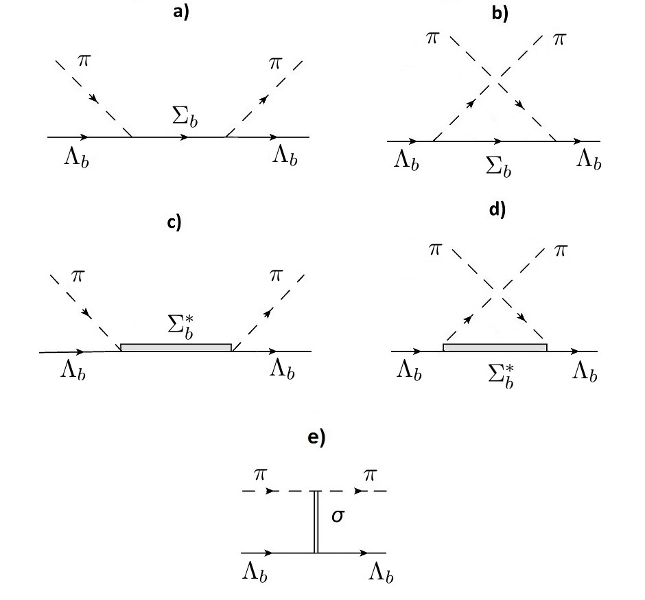
Figure 1: Diagrams to be considered in the $\pi\Lambda_{b}$ interaction

Table 1: Resonances considered in $\pi\Lambda_{b}$ interaction

	$J^{\pi}$	$I$	$Mass$ $(MeV)$
$\Sigma_{b}$	$1/2^{+}$	1	5812
$\Sigma_{b}^{*}$	$3/2^{+}$	1	5832

The interaction with a $\Sigma_{b}$ spin-1/2 baryon in the intermediate state will be studied in Sec. III.1 and the $\Sigma_{b}^{*}$ spin-3/2 pole in Sec. III.2. The amplitude for the the scalar $\sigma$ meson exchange shown in Fig. 1$e$, will be included as a parametrization as it has been made in BH -ccb . So the amplitudes to be considered are

$$A_{\sigma}=a+bt\ ,$$ (10)

$$B_{\sigma}=0\ ,$$ (11)

with $a=1.05m_{\pi}^{-1}$, $b=-0.8m_{\pi}^{-3}$ where $m_{\pi}$ is the pion mass pdg and $t$ a is the Mandelstam variable defined in the Appendix. More discussions about these amplitudes may be found in cm , leut1 -r1 . From these results the partial-wave amplitudes $f_{l\pm}$ for the diagrams of Fig. 1 may be calculated.

III.1 $\Sigma_{b}$ baryon

In order to study the $\pi\Lambda_{b}$ interactions, the Lagrangians (1) and (II) will be adapted considering the pion and the $\Lambda_{b}$ as initial particles with $\Sigma_{b}$ (spin-1/2) and $\Sigma_{b}^{*}$ (spin-3/2) in the intermediate states. Thus the Lagrangian (1) will be written as

$$\mathcal{L}_{\pi\Lambda_{b}\Sigma_{b}}=\frac{g_{\pi\Lambda_{b}\Sigma_{b}}}{2m_{\Lambda_{b}}}\big{(}\overline{\vec{\Sigma}_{b}}\gamma_{\mu}\gamma_{5}\Lambda_{b}\big{)}\cdot\partial^{\mu}\vec{\phi}\ ,$$ (12)

which determines the vertex

$$V_{\pi\Lambda_{b}\Sigma_{b}}=\frac{g_{\pi\Lambda_{b}\Sigma_{b}}}{2m_{\Lambda_{b}}}\not{k}\gamma_{5}\ ,$$ (13)

where $g_{\pi\Lambda_{b}\Sigma_{b}}$ is the coupling constant for the $\pi\Lambda_{b}\Sigma_{b}$ interaction and $m_{\Lambda_{b}}$ is the $\Lambda_{b}$ mass.

Calculating the contribution of the diagrams $a$ and $b$ of Fig. 1 to the $T_{\pi\Lambda_{b}}$ amplitude, relative to the process $\pi\Lambda_{b}\rightarrow\pi\Lambda_{b}$ and writing them in the form of eq.(3) we have

$$A_{\Sigma_{b}} = \frac{g_{\pi\Lambda_{b}\Sigma_{b}}^{2}}{4m_{\Lambda_{b}}^{2}}(m_{\Sigma_{b}}+m_{\Lambda_{b}})\bigg{(}\frac{s-m_{\Lambda_{b}}^{2}}{s-m_{\Sigma_{b}}^{2}}+\frac{u-m_{\Lambda_{b}}^{2}}{u-m_{\Sigma_{b}}^{2}}\bigg{)}\ ,$$

$$B_{\Sigma_{b}} = \frac{g_{\pi\Lambda_{b}\Sigma_{b}}^{2}}{4m_{\Lambda_{b}}^{2}}\bigg{[}\frac{2m_{\Lambda_{b}}(m_{\Lambda_{b}}+m_{\Sigma_{b}})+u-m_{\Lambda_{b}}^{2}}{u-m_{\Sigma_{b}}^{2}}$$ (15)

$$-\frac{2m_{\Lambda_{b}}(m_{\Lambda_{b}}+m_{\Sigma_{b}})+s-m_{\Lambda_{b}}^{2}}{s-m_{\Sigma_{b}}^{2}}\bigg{]}\ ,$$

where $u$ is a Mandelstam variable and $m_{\Sigma_{b}}$ is the $\Sigma_{b}$ mass.

Using eq. (III.1) and (15) in eq. (8) we have

$$f_{1} = \frac{g^{2}_{\pi\Lambda_{b}\Sigma_{b}}(E+m_{\Lambda_{b}})}{32\pi m_{\Lambda_{b}}^{2}\sqrt{s}}\bigg{\{}\frac{1}{s-m_{\Sigma_{b}}^{2}}\bigg{[}(m_{\Sigma_{b}}+2m_{\Lambda_{b}}$$ (16)

$$-\sqrt{s})(s-m_{\Lambda_{b}}^{2})+2m_{\Lambda_{b}}(m_{\Lambda_{b}}+m_{\Sigma_{b}})(m_{\Lambda_{b}}-\sqrt{s})\bigg{]}$$

$$+\frac{1}{u-m_{\Sigma_{b}}^{2}}\bigg{[}2m_{\Lambda_{b}}(m_{\Lambda_{b}}+m_{\Sigma_{b}})(\sqrt{s}-m_{\Lambda_{b}})$$

$$+(m_{\Sigma_{b}}+\sqrt{s})(u-m_{\Lambda_{b}}^{2})\bigg{]}\bigg{\}}\ .$$

Considering eq. (44) and (45) defined in Appendix, is convenient write the $f_{1}$ amplitude as function of $x=\cos\theta$

$$f_{1}=\frac{g^{2}_{\pi\Lambda_{b}\Sigma_{b}}(E+m_{\Lambda_{b}})}{32\pi m_{\Lambda_{b}}^{2}\sqrt{s}}\bigg{\{}a_{1}+\frac{b_{1}+c_{1}x}{\gamma_{\Sigma_{b}}+2|\vec{k}|^{2}x}\bigg{\}}\ ,$$ (17)

where

$$a_{1} = \tfrac{(m_{\Sigma_{b}}+2m_{\Lambda_{b}}-\sqrt{s})(s-m_{\Lambda_{b}}^{2})+2m_{\Lambda_{b}}(m_{\Lambda_{b}}+m_{\Sigma_{b}})(m_{\Lambda_{b}}-\sqrt{s})}{s-m_{\Sigma_{b}}^{2}};$$

$$b_{1} = 2m_{\Lambda_{b}}(m_{\Lambda_{b}}+m_{\Sigma_{b}})(m_{\Lambda_{b}}-\sqrt{s})$$

$$+(m_{\Sigma_{b}}+\sqrt{s})(2Ek_{0}-m_{\pi}^{2});$$

$$c_{1} = 2|\vec{k}|^{2}(\sqrt{s}+m_{\Sigma_{b}});$$

$$\gamma_{\Sigma_{b}} = m_{\Sigma_{b}}^{2}-m_{\Lambda_{b}}^{2}-m_{\pi}^{2}+2Ek_{0}.$$

and $k_{0}$ is the pion energy.

From (III.1), (15) and (9), we have

$$f_{2} = \frac{g^{2}_{\pi\Lambda_{b}\Sigma_{b}}(E-m_{\Lambda_{b}})}{32\pi m_{\Lambda_{b}}^{2}\sqrt{s}}\bigg{\{}\frac{1}{s-m_{\Sigma_{b}}^{2}}\bigg{[}(m_{\Sigma_{b}}+2m_{\Lambda_{b}}+\sqrt{s})(m_{\Lambda_{b}}^{2}-s)$$ (18)

$$-2m_{\Lambda_{b}}(m_{\Lambda_{b}}+m_{\Sigma_{b}})(m_{\Lambda_{b}}+\sqrt{s})\bigg{]}$$

$$+\frac{1}{u-m_{\Sigma_{b}}^{2}}\bigg{[}2m_{\Lambda_{b}}(m_{\Lambda_{b}}+m_{\Sigma_{b}})(m_{\Lambda_{b}}+\sqrt{s})$$

$$+(\sqrt{s}-m_{\Sigma_{b}})(u-m_{\Lambda_{b}}^{2})\bigg{]}\bigg{\}}\ ,$$

and following the same procedure that has been followed in the calculation of $f_{1}$ we obtain

$$f_{2}=\frac{g^{2}_{\pi\Lambda_{b}\Sigma_{b}}(E-m_{\Lambda_{b}})}{32\pi m_{\Lambda_{b}}^{2}\sqrt{s}}\bigg{\{}a_{2}+\frac{b_{2}+c_{2}x}{\gamma_{\Sigma_{b}}+2|\vec{k}|^{2}x}\bigg{\}}\ ,$$ (19)

where

$$a_{2} = \tfrac{(m_{\Sigma_{b}}+2m_{\Lambda_{b}}+\sqrt{s})(m_{\Lambda_{b}}^{2}-s)-2m_{\Lambda_{b}}(m_{\Lambda_{b}}+m_{\Sigma_{b}})(m_{\Lambda_{b}}+\sqrt{s})}{s-m_{\Sigma_{b}}^{2}};$$

$$b_{2} = -2m_{\Lambda_{b}}(m_{\Lambda_{b}}+m_{\Sigma_{b}})(\sqrt{s}+m_{\Lambda_{b}})+(\sqrt{s}-m_{\Sigma_{b}})(2Ek_{0}-m_{\pi}^{2});$$

$$c_{2} = 2|\vec{k}|^{2}(\sqrt{s}-m_{\Sigma_{b}}).$$

Thus, using eqs. (17) and (62) in eq. (7) the $S$, $P_{1}$ and $P_{3}$ partial-waves amplitudes may be calculated

$$a_{S}^{({\Sigma_{b}})} = \frac{g^{2}_{\pi\Lambda_{b}\Sigma_{b}}}{64\pi m_{\Lambda_{b}}^{2}\sqrt{s}}\bigg{\{}2(E+m_{\Lambda_{b}})a_{1}+(E+m_{\Lambda_{b}})b_{1}I_{0}$$ (20)

$$+\Big{[}(E+m_{\Lambda_{b}})c_{1}+(E-m_{\Lambda_{b}})b_{2}\Big{]}I_{1}$$

$$+(E-m_{\Lambda_{b}})c_{2}I_{2}\bigg{\}}\ ,$$

$$a_{P_{1}}^{({\Sigma_{b}})} = \frac{g^{2}_{\pi\Lambda_{b}\Sigma_{b}}}{64\pi m_{\Lambda_{b}}^{2}\sqrt{s}}\bigg{\{}2(E-m_{\Lambda_{b}})a_{2}+(E-m_{\Lambda_{b}})b_{2}I_{0}$$ (21)

$$+\Big{[}(E+m_{\Lambda_{b}})b_{1}+(E-m_{\Lambda_{b}})c_{2}\Big{]}I_{1}$$

$$+(E+m_{\Lambda_{b}})c_{1}I_{2}\bigg{\}}\ ,$$

$$a_{P_{3}}^{({\Sigma_{b}})} = \frac{g^{2}_{\pi\Lambda_{b}\Sigma_{b}}}{64\pi m_{\Lambda_{b}}^{2}\sqrt{s}}\bigg{\{}\Big{(}\frac{m_{\Lambda_{b}}-E}{2}\Big{)}b_{2}I_{0}$$ (22)

$$+\Big{[}(E+m_{\Lambda_{b}})b_{1}+\Big{(}\frac{m_{\Lambda_{b}}-E}{2}\Big{)}c_{2}\Big{]}I_{1}$$

$$+\Big{[}\frac{3}{2}(E-m_{\Lambda_{b}})b_{2}+(E+m_{\Lambda_{b}})c_{1}\Big{]}I_{2}$$

$$+\frac{3}{2}(E-m_{\Lambda_{b}})c_{2}I_{3}\bigg{\}}\ ,$$

where $I_{0}$, $I_{1}$, $I_{2}$ and $I_{3}$ are integrals defined in the Appendix.

These amplitudes will be used in Sec. IV in order to calculate the observables of interest.

III.2 $\Sigma_{b}^{*}$ baryon

Now, adapting the Lagrangian (II) in order to describe a the spin-3/2 $\Sigma_{b}^{*}$ resonance in the intermediate state, represented in the diagrams $c$ and $d$ of Fig.1, we have

$$\mathcal{L}_{\pi\Lambda_{b}{\Sigma^{*}_{b}}}=g_{\pi\Lambda_{b}\Sigma^{*}_{b}}\Big{\{}\overline{{\vec{\Sigma}_{b}}^{*\mu}}\big{[}g_{\mu\nu}-(Z+1/2)\gamma_{\mu}\gamma_{\nu}\big{]}\Lambda_{b}\Big{\}}\cdot\partial^{\nu}\vec{\phi}\ ,$$ (23)

as the $\Lambda_{b}$ hyperon has isospin 0, the isospin matrix $\vec{M}$ in eq. (II) is not needed. So, the Feynman vertex is

$$V_{\pi\Lambda_{b}{\Sigma^{*}_{b}}}=g_{\pi\Lambda_{b}{\Sigma^{*}_{b}}}\Big{[}k^{\mu}-(Z+1/2)\gamma^{\mu}\not{k}\Big{]}\ ,$$ (24)

and then the amplitudes are

$$A_{\Sigma^{*}_{b}} = \frac{2g_{\pi\Lambda_{b}{\Sigma^{*}_{b}}}^{2}}{9m_{\Lambda_{b}}}\bigg{[}\frac{\nu_{\Sigma^{*}_{b}}}{\nu_{\Sigma^{*}_{b}}^{2}-\nu^{2}}\hat{A}+m_{\Lambda_{b}}(-a_{0}+a_{z}k.k^{\prime})\bigg{]}\ ,$$

$$B_{\Sigma^{*}_{b}} = \frac{2g_{\pi\Lambda_{b}{\Sigma^{*}_{b}}}^{2}}{9m_{\Lambda_{b}}}\bigg{[}\frac{\nu}{\nu_{\Sigma^{*}_{b}}^{2}-\nu^{2}}\hat{B}-(2m_{\Lambda_{b}}^{2}b_{0})\nu\bigg{]}\ ,$$ (26)

where $g_{\pi\Lambda_{b}\Sigma^{*}_{b}}$ is the coupling constant and $\nu$, $\nu_{\Sigma_{b}^{*}}$ and $k.k^{\prime}$ are defined in the Appendix. The other terms that appear in eq. (III.2) and (26) are defined as

$$\hat{A} = \frac{(m_{\Sigma^{*}_{b}}+m_{\Lambda_{b}})^{2}-m_{\pi}^{2}}{2m_{\Sigma^{*}_{b}}^{2}}\bigg{[}2m_{\Sigma^{*}_{b}}^{3}-2m_{\Lambda_{b}}^{3}-2m_{\Lambda_{b}}m_{\Sigma^{*}_{b}}^{2}$$ (27)

$$-2m_{\Lambda_{b}}^{2}m_{\Sigma^{*}_{b}}+m_{\pi}^{2}(2m_{\Lambda_{b}}-m_{\Sigma^{*}_{b}})\bigg{]}$$

$$+\frac{3}{2}(m_{\Lambda_{b}}+m_{\Sigma^{*}_{b}})t\ ,$$

$$\hat{B} = \frac{1}{2m_{\Sigma^{*}_{b}}^{2}}\bigg{[}(m_{\Sigma^{*}_{b}}^{2}-m_{\Lambda_{b}}^{2})^{2}$$ (28)

$$-2m_{\Lambda_{b}}m_{\Sigma^{*}_{b}}(m_{\Lambda_{b}}+m_{\Sigma^{*}_{b}})^{2}-2m_{\pi}^{2}(m_{\Lambda_{b}}+m_{\Sigma^{*}_{b}})^{2}$$

$$+6m_{\pi}^{2}m_{\Sigma^{*}_{b}}(m_{\Lambda_{b}}+m_{\Sigma^{*}_{b}})+m_{\pi}^{4}\bigg{]}+\frac{3}{2}t\ ,$$

$$a_{0} = \frac{(m_{\Lambda_{b}}+m_{\Sigma^{*}_{b}})}{m_{\Sigma^{*}_{b}}^{2}}(2m_{\Sigma^{*}_{b}}^{2}+m_{\Lambda_{b}}m_{\Sigma^{*}_{b}}-m_{\Lambda_{b}}^{2}+2m_{\pi}^{2})\ ,$$

$$a_{z} = \frac{4}{m_{\Sigma^{*}_{b}}^{2}}\Big{[}(m_{\Sigma^{*}_{b}}+m_{\Lambda_{b}})Z+(2m_{\Sigma^{*}_{b}}+m_{\Lambda_{b}})Z^{2}\Big{]}\ ,$$ (30)

$$b_{0} = \frac{4Z^{2}}{m_{\Sigma^{*}_{b}}^{2}}\ ,$$ (31)

where $m_{\Sigma_{b}^{*}}$ is the resonance mass.

Then, substituting (III.2) and (26) in the eq. (8), we find

$$f_{1} = \frac{g_{\pi\Lambda_{b}{\Sigma^{*}_{b}}}^{2}}{9}\frac{(E+m_{\Lambda_{b}})}{4\pi\sqrt{s}}\bigg{\{}\frac{\hat{A}+(\sqrt{s}-m_{\Lambda_{b}})\hat{B}}{m_{\Sigma^{*}_{b}}^{2}-s}$$ (32)

$$+\frac{\hat{A}+(m_{\Lambda_{b}}-\sqrt{s})\hat{B}}{m_{\Sigma^{*}_{b}}^{2}-u}-a_{0}+a_{z}kk^{\prime}$$

$$-2m_{\Lambda_{b}}(\sqrt{s}-m_{\Lambda_{b}})b_{0}\nu\bigg{\}}\ ,$$

that in terms of $x$ may be written as

$$f_{1}=\frac{g_{\pi\Lambda_{b}{\Sigma^{*}_{b}}}^{2}(E+m_{\Lambda_{b}})}{36\pi\sqrt{s}}\bigg{\{}\alpha_{1}+\beta_{1}x+\frac{a_{1}+b_{1}x}{\gamma_{\Sigma^{*}_{b}}+2|\vec{k}|^{2}x}\bigg{\}}\ ,$$ (33)

where

$$\alpha_{1} = \frac{3(\sqrt{s}+m_{\Sigma^{*}_{b}})}{4m_{\Sigma^{*}_{b}}^{2}s}\Big{[}m_{\Sigma^{*}_{b}}^{2}s-(m_{\Lambda_{b}}^{2}-m_{\pi}^{2})^{2}\Big{]}+\frac{(E_{\Sigma^{*}_{b}}+m_{\Lambda_{b}})^{2}}{\sqrt{s}+m_{\Sigma^{*}_{b}}}$$

$$-a_{0}+a_{z}k_{0}^{2}+b_{0}(m_{\Lambda_{b}}-\sqrt{s})(2Ek_{0}+|\vec{k}|^{2});$$

$$\beta_{1} = \frac{3|\vec{k}|^{2}}{m_{\Sigma^{*}_{b}}-\sqrt{s}}-\Big{[}a_{z}-(m_{\Lambda_{b}}-\sqrt{s})b_{0}\Big{]}|\vec{k}|^{2};$$

$$a_{1} = 3(2m_{\Lambda_{b}}+m_{\Sigma^{*}_{b}}-\sqrt{s})(|\vec{q}_{\Sigma^{*}_{b}}|^{2}-|\vec{k}|^{2})$$

$$+(m_{\Sigma^{*}_{b}}-2m_{\Lambda_{b}}+\sqrt{s})(E_{\Sigma^{*}_{b}}+m_{\Lambda_{b}})^{2};$$

$$b_{1} = 3|\vec{k}|^{2}(2m_{\Lambda_{b}}+m_{\Sigma^{*}_{b}}-\sqrt{s});$$

$$\gamma_{\Sigma_{b}^{*}} = m_{\Sigma^{*}_{b}}^{2}-m_{\Lambda_{b}}^{2}-m_{\pi}^{2}+2Ek_{0}.$$

For the $f_{2}$ amplitude we have

$$f_{2} = \frac{g_{\pi\Lambda_{b}{\Sigma^{*}_{b}}}^{2}}{9}\frac{(E-m_{\Lambda_{b}})}{4\pi\sqrt{s}}\bigg{\{}\frac{-\hat{A}+(\sqrt{s}+m_{\Lambda_{b}})\hat{B}}{m_{\Sigma^{*}_{b}}^{2}-s}$$ (34)

$$-\frac{\hat{A}+(\sqrt{s}+m_{\Lambda_{b}})\hat{B}}{m_{\Sigma^{*}_{b}}^{2}-u}+a_{0}-a_{z}kk^{\prime}$$

$$-2m_{\Lambda_{b}}(\sqrt{s}+m_{\Lambda_{b}})b_{0}\nu\bigg{\}}\ ,$$

then,

$$f_{2}=\frac{g_{\pi\Lambda_{b}{\Sigma^{*}_{b}}}^{2}(E-m_{\Lambda_{b}})}{36\pi\sqrt{s}}\bigg{\{}\alpha_{2}+\beta_{2}x-\frac{a_{2}+b_{2}x}{\gamma_{\Sigma^{*}_{b}}+2|\vec{k}|^{2}x}\bigg{\}}\ ,$$ (35)

where

$$\alpha_{2} = -3\frac{|\vec{q}_{\Sigma^{*}_{b}}|^{2}-|\vec{k}|^{2}}{\sqrt{s}+m_{\Sigma^{*}_{b}}}+\frac{(E_{\Sigma^{*}_{b}}+m_{\Lambda_{b}})^{2}}{\sqrt{s}-m_{\Sigma^{*}_{b}}}$$

$$+a_{0}-a_{z}k_{0}^{2}-b_{0}(\sqrt{s}+m_{\Lambda_{b}})(2Ek_{0}+|\vec{k}|^{2});$$

$$\beta_{2} = \frac{-3|\vec{k}|^{2}}{m_{\Sigma^{*}_{b}}+\sqrt{s}}+\Big{[}a_{z}-(m_{\Lambda_{b}}+\sqrt{s})b_{0}\Big{]}|\vec{k}|^{2};$$

$$a_{2} = 3(2m_{\Lambda_{b}}+m_{\Sigma^{*}_{b}}+\sqrt{s})(|\vec{q}_{\Sigma^{*}_{b}}|^{2}-|\vec{k}|^{2})$$

$$+(m_{\Sigma^{*}_{b}}-2m_{\Lambda_{b}}-\sqrt{s})(E_{\Sigma^{*}_{b}}+m_{\Lambda_{b}})^{2};$$

$$b_{2} = 3|\vec{k}|^{2}(2m_{\Lambda_{b}}+m_{\Sigma^{*}_{b}}+\sqrt{s})\ .$$

Finally, the resulting partial-waves $S$ and $P$ amplitudes are

$$a_{S}^{({\Sigma_{b}^{*}})} = \frac{g^{2}_{\pi\Lambda_{b}{\Sigma^{*}_{b}}}}{72\pi\sqrt{s}}\bigg{\{}2(E+m_{\Lambda_{b}})\alpha_{1}+\frac{2}{3}(E-m_{\Lambda_{b}})\beta_{2}$$ (36)

$$+(E+m_{\Lambda_{b}})a_{1}I_{0}+\Big{[}(E+m_{\Lambda_{b}})b_{1}-(E-m_{\Lambda_{b}})a_{2}\Big{]}I_{1}$$

$$-(E-m_{\Lambda_{b}})b_{2}I_{2}\bigg{\}}\ ,$$

$$a_{P_{1}}^{({\Sigma_{b}^{*}})} = \frac{g^{2}_{\pi\Lambda_{b}{\Sigma^{*}_{b}}}}{72\pi\sqrt{s}}\bigg{\{}2(E-m_{\Lambda_{b}})\alpha_{2}+\frac{2}{3}(E+m_{\Lambda_{b}})\beta_{1}$$ (37)

$$-(E-m_{\Lambda_{b}})a_{2}I_{0}+\Big{[}(E+m_{\Lambda_{b}})a_{1}-(E-m_{\Lambda_{b}})b_{2}\Big{]}I_{1}$$

$$+(E+m_{\Lambda_{b}})b_{1}I_{2}\bigg{\}}\ ,$$

$$a_{P_{3}}^{({\Sigma_{b}^{*}})} = \frac{g^{2}_{\pi\Lambda_{b}{\Sigma^{*}_{b}}}}{72\pi\sqrt{s}}\bigg{\{}\frac{2}{3}(E+m_{\Lambda_{b}})\beta_{1}-\Big{(}\frac{m_{\Lambda_{b}}-E}{2}\Big{)}a_{2}I_{0}$$ (38)

$$+\Big{[}(E+m_{\Lambda_{b}})a_{1}-\Big{(}\frac{m_{\Lambda_{b}}-E}{2}\Big{)}b_{2}\Big{]}I_{1}$$

$$+\Big{[}\frac{3}{2}(m_{\Lambda_{b}}-E)a_{2}+(E+m_{\Lambda_{b}})b_{1}\Big{]}I_{2}$$

$$+\frac{3}{2}(m_{\Lambda_{b}}-E)b_{2}I_{3}\bigg{\}}\ .$$

IV Results

Considering the amplitudes obtained before, now it is possible to calculate the observables of interest, that is the subject of this section. First of all we must observe that the calculated partial-wave amplitudes are real, and then violate the unitarity of the $S$ matrix. These amplitudes may be unitarized BH -cm with

$$a_{l\pm}^{U}=\frac{a_{\pm}}{1-i|\vec{k}|a_{\pm}}\ .$$ (39)

In the center-of-mass frame the differential cross section is given by

$$\frac{d\sigma}{d\Omega}=|f|^{2}+|g|^{2}\ ,$$ (40)

and the total cross section may be obtained by integrating this expression over the solid angle that results in

$$\sigma_{T}=4\pi\sum_{l}{\Big{[}(l+1)|a_{l+}^{U}|^{2}+l|a_{l-}^{U}|^{2}\Big{]}}\ .$$ (41)

The polarization is defined by

$$\vec{P}=-2\frac{{\rm Im}(f^{*}g)}{|f|^{2}+|g|^{2}}\hat{n}\ ,$$ (42)

where $\hat{n}$ is a unitary vector normal to the scattering plane and the phase shifts are given by

$$\delta_{l\pm}=\tan^{-1}(|\vec{k}|a_{\pm})\ .$$ (43)

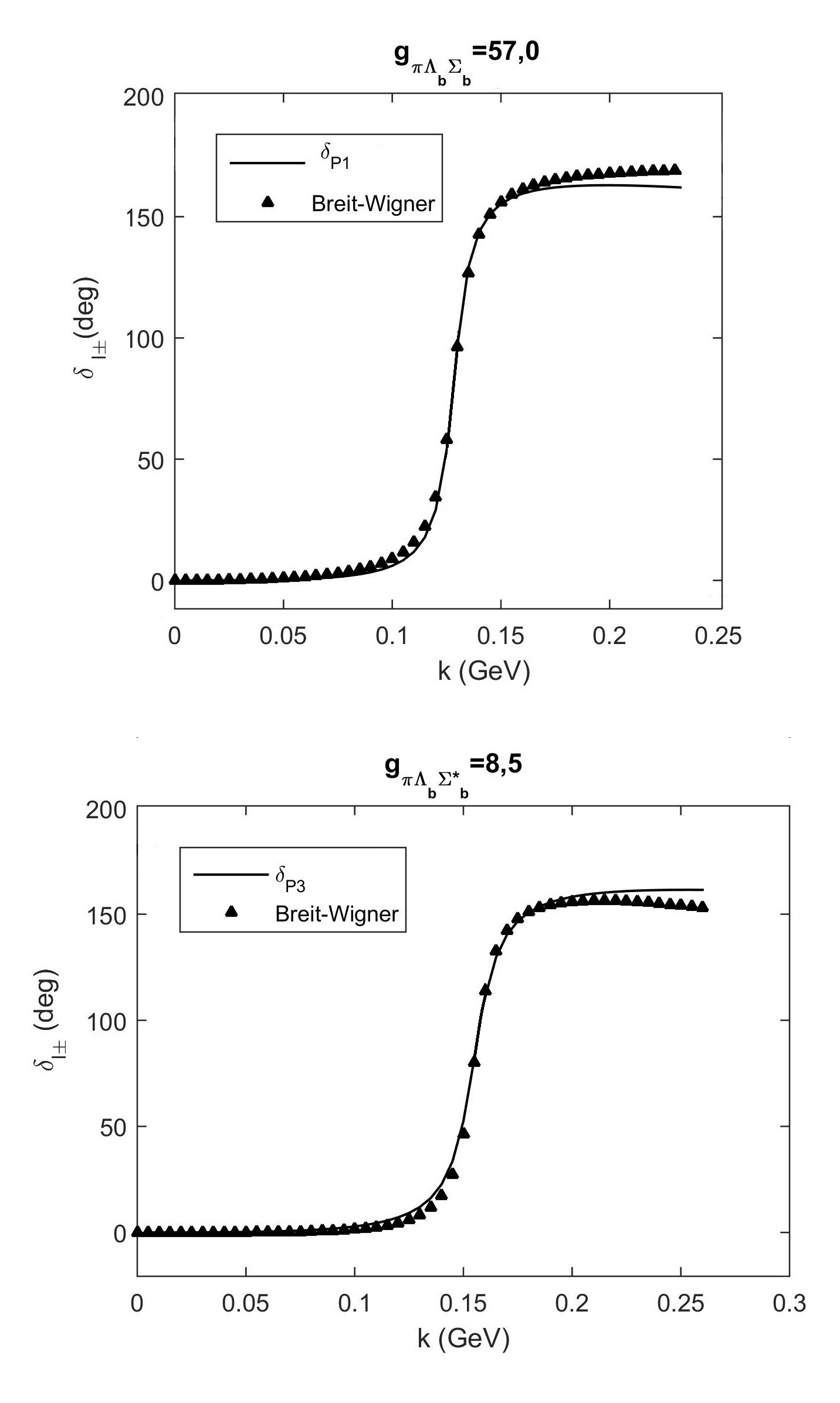
Figure 2: Breit-Wigner fit for the $\Sigma_{b}$ and $\Sigma_{b}^{*}$ resonances

The parameters used in the calculations are shown in Tab. 1 and 2. The coupling constants have been determined by comparing our results for the phase-shifts with the Breit-Wigner expression (see the Appendix) BH , sant , as it is shown in Fig. 2. In Fig. 3, 4, 5 and 6 the total cross section, phase-shifts, differential cross section and polarization are plotted as functions of the pion momentum $k=|\vec{k}|$ and $x$. The gaps between the lines in Fig. 6, for the polarization, are 10 $MeV$.

Table 2: Constants of $\pi\Lambda_{b}$ interaction

$m_{\Lambda_{b}}$	$5620$ $MeV$
$g_{\pi\Lambda_{b}\Sigma_{b}}$	$63.0$ $GeV^{-1}$
$g_{\pi\Lambda_{b}\Sigma_{b}^{*}}$	$8.5$ $GeV^{-1}$
$Z$	-0.5

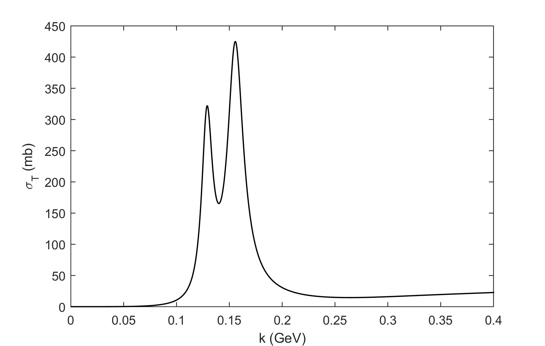
Figure 3: Total Cross Section of the $\pi\Lambda_{b}$ interaction

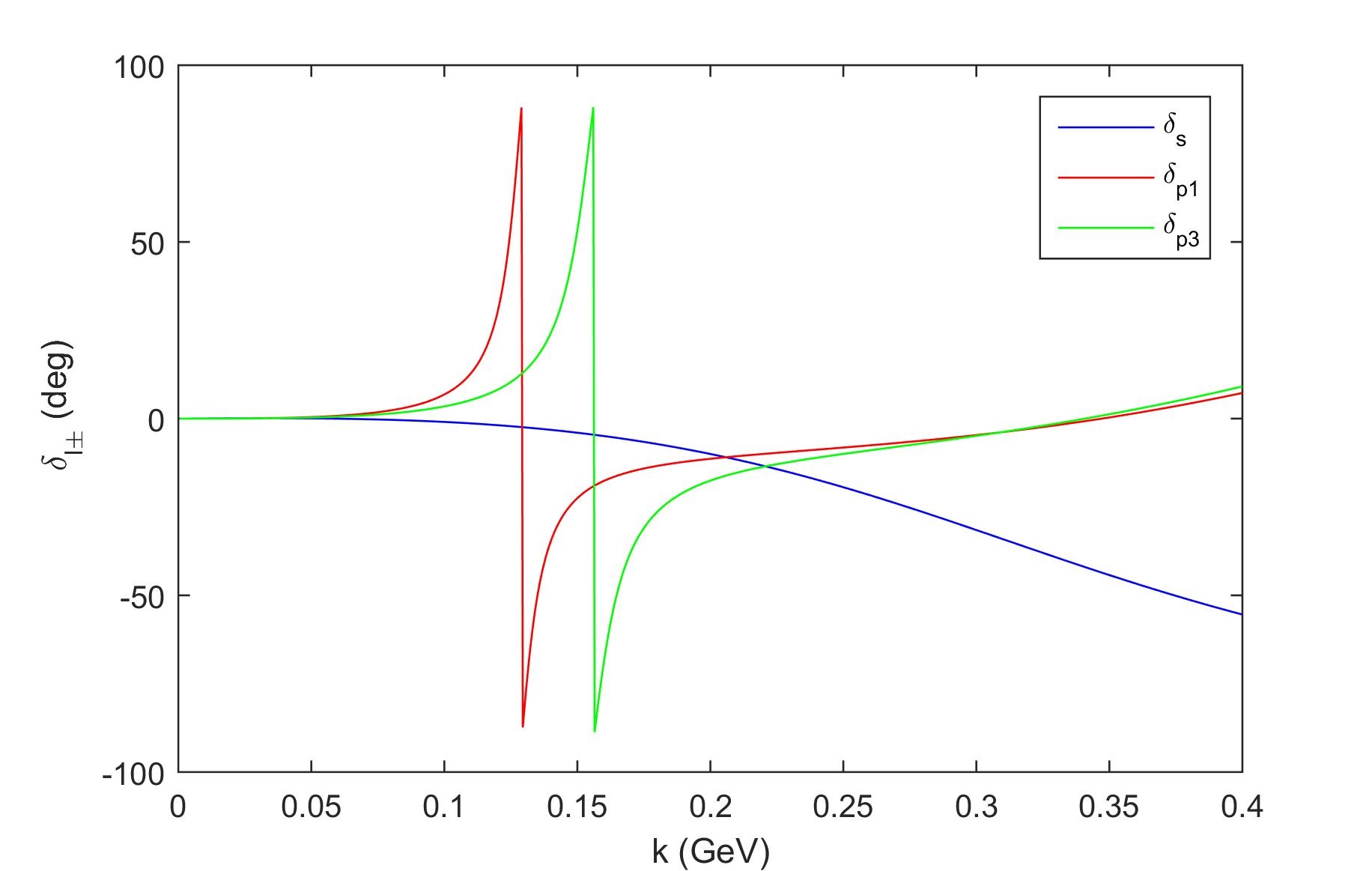
Figure 4: Phase Shifts of the $\pi\Lambda_{b}$ interaction

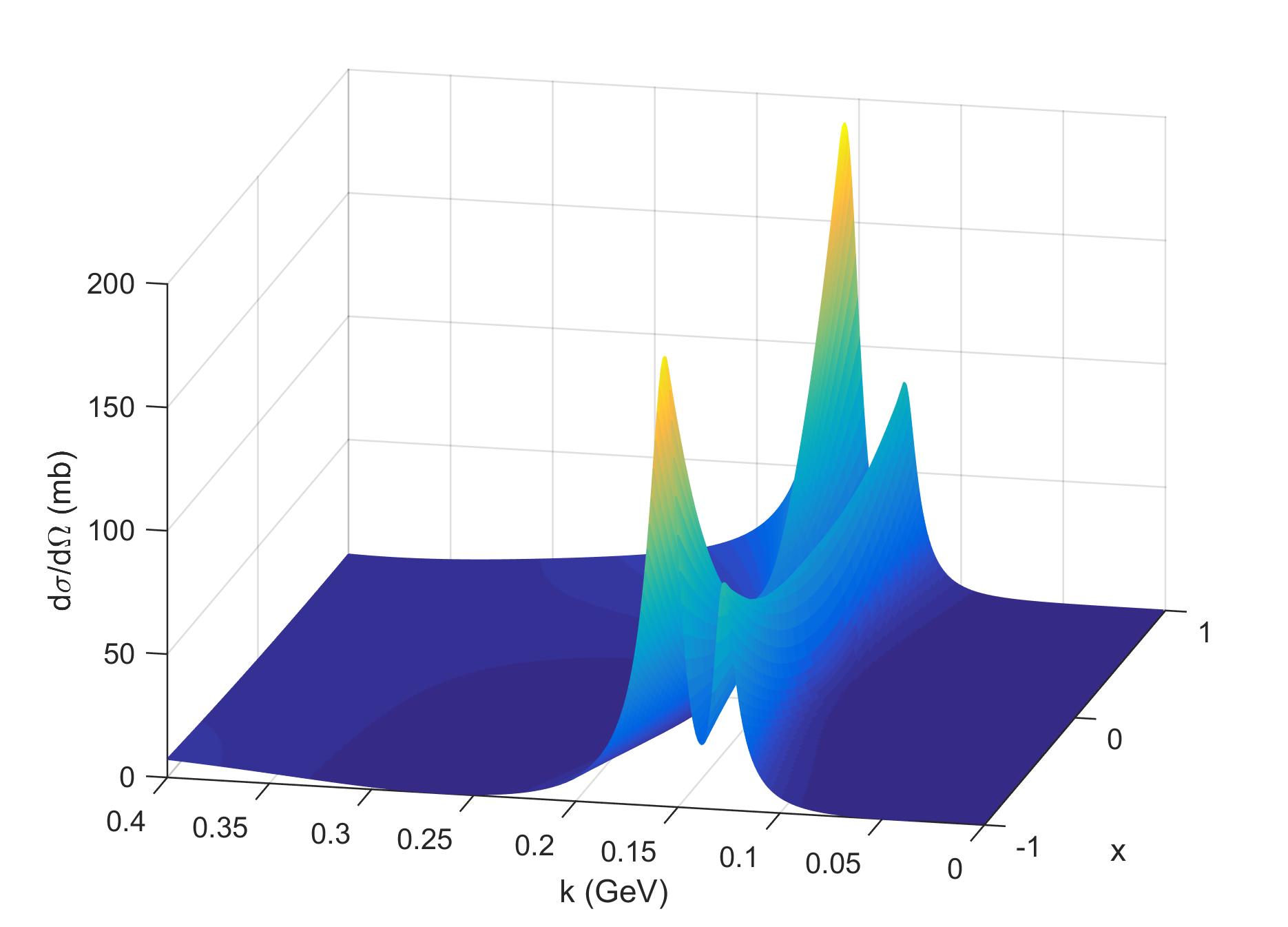
Figure 5: Differential Cross Section of the $\pi\Lambda_{b}$ interaction

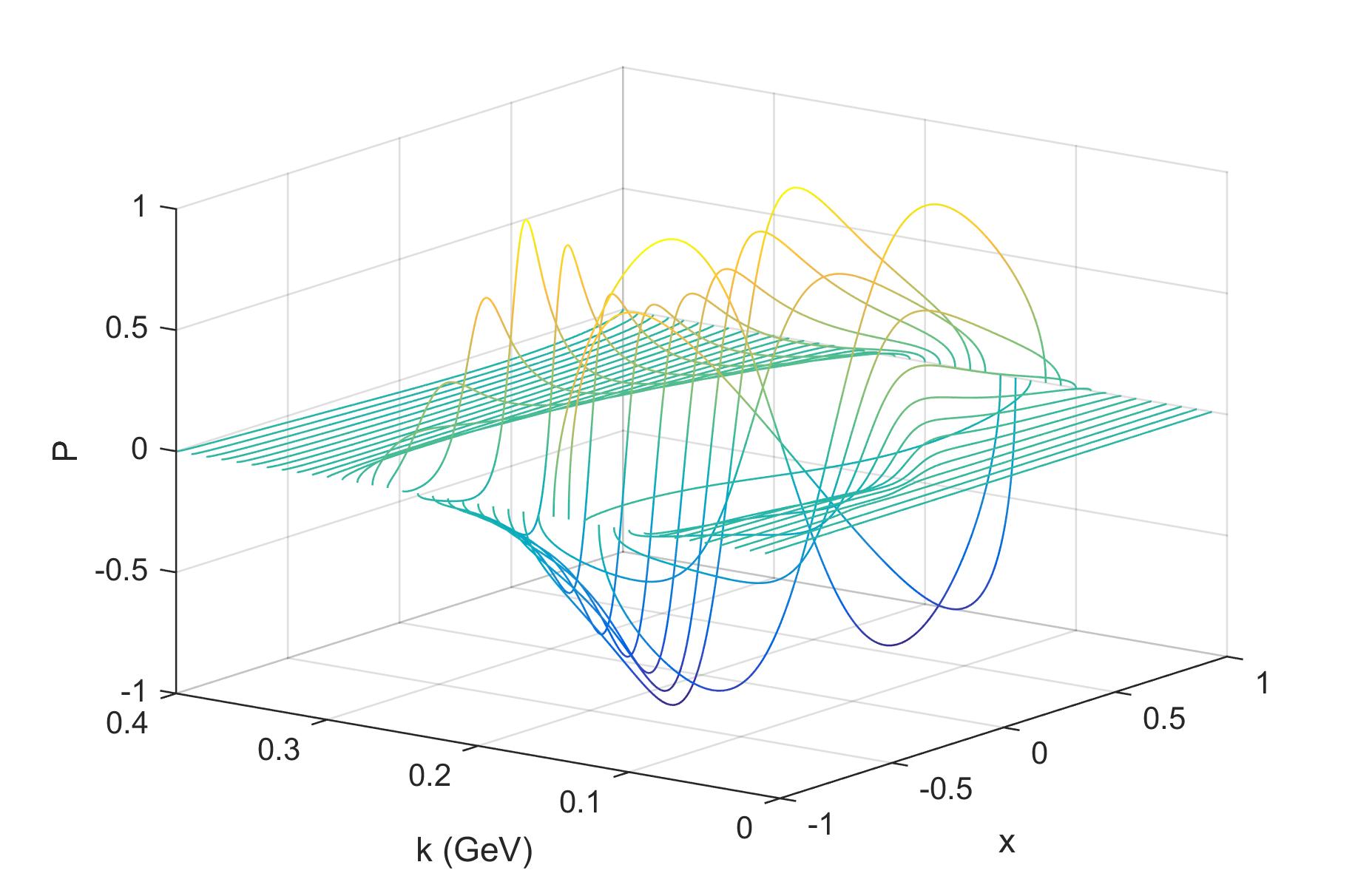
Figure 6: Polarization in the $\pi\Lambda_{b}$ interaction

V Conclusions

In this work the low energy pion-$\Lambda_{b}$ has been studied. We considered Lagrangians that include pions, $\Lambda_{b}$, $\Sigma_{b}$ and $\Sigma_{b}^{*}$. In the interaction mediated by $\sigma$, a parametrization has been considered. The coupling constants have been determined and then the phase-shifts, cross-sections and polarizations have been calculated. As it should be expected, at low energies, the resonances dominate the cross sections, as it may be seen in Fig. 3 and 5. This behavior is similar to the one observed in pion-hyperon BH -cm and kaon-hyperon sant , sant2 interactions and is very well determined in the pion-nucleon interactions, where the $\Delta$ particle dominates the cross section in the spin-3/2 and isospin-3/2 channel.

At the LHCb experiment lhcb , the transverse polarization of $\Lambda_{b}$ at $\sqrt{s}$= 7 TeV has been measured 0.06$\pm$0.07$\pm$0.02 and in the CMS cms , for $\sqrt{s}$ =7 and 8 TeV, the measured polarization was 0.00$\pm$0.06$\pm$0.06, that are small values. Observing Fig. 6, we may see that in general, the polarization is not so large, except near the $\Sigma_{b}$ and $\Sigma_{b}^{*}$ masses. If this polarization is considered in mechanisms such as the ones presented in cy -ccb2 , that take into account the final-state interactions of the $\Lambda_{b}$, a relatively small value of the polarization $1\%-2\%$ (or even smaller) should remain when the average is computed. Obviously in order to determine the exact value, the calculations must be made, that is a task for a future work.

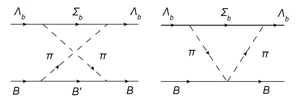
Figure 7: Examples of two pions exchange in the $Y\Lambda_{b}$ or $N\Lambda_{b}$ interactions

The results of this work are also important in the determination of nucleon-$\Lambda_{b}$ and hyperon-$\Lambda_{b}$ potentials, as the pion-$\Lambda_{b}$ interaction is needed in order to calculate diagrames of the type of Fig. 7. This kind of potential is fundamental in many physical systems, as for example in order to describe exotic nuclei that contain bottom baryons. Then, the model presented in this work deals with an important aspect of physics, where still there are much to be done, that is describing and understanding the interactions and proprieties of the heavy-quark baryons.

VI Acknowledgments

This study has been partially supported by the Coordenação de Aperfeiçoamento de Pessoal de Nível Superior (CAPES) – Finance Code 001.

VII Appendix

VII.1 Kinematics Relations

Considering a process where $p_{\mu}$ and $p_{\mu}^{\prime}$ are the initial and final baryon four-momenta, $k_{\mu}$ and $k_{\mu}^{\prime}$ are the initial and final meson four-momenta, the Mandelstam variables may be written in terms of variables defined in the center-of-mass frame, $|\vec{k}|$ is the three-momentum absolute value of the incident particle and $\theta$, the scattering angle

$$s=(p+k)^{2}=(p^{\prime}+k^{\prime})^{2}=m^{2}_{\Lambda_{b}}+m_{\pi}^{2}+2Ek_{0}-2\vec{k}.\vec{p}\ ,$$

$$s=m_{\Lambda_{b}}^{2}+m_{\pi}^{2}+2Ek_{0}+2{|\vec{k}|}^{2}\ ,$$ (44)

$$u=(p^{\prime}-k)^{2}=(p-k^{\prime})^{2}=m^{2}_{\Lambda_{b}}+m_{\pi}^{2}-2Ek_{0}-2\vec{k}^{\prime}.\vec{p}\ ,$$

$$u=m^{2}_{\Lambda_{b}}+m_{\pi}^{2}-2{|\vec{k}|}^{2}x-2Ek_{0}\ ,$$ (45)

$$t=(p-p^{\prime})^{2}=(k-k^{\prime})^{2}=2|\vec{k}|^{2}x-2|\vec{k}|^{2}\ .$$

$$t=2|{\vec{k}}|^{2}(x-1)\ ,$$ (46)

where

$$x=\cos\theta\ ,$$ (47)

and the energies are defined as

$$k_{0}=k^{\prime}_{0}=\sqrt{|\vec{k}|^{2}+m_{\pi}^{2}}\ ,$$ (48)

$$E=E^{\prime}=\sqrt{|\vec{k}|^{2}+m^{2}_{\Lambda_{b}}}\ ,$$ (49)

also

$$E+k_{0}=\sqrt{s}\ ,$$ (50)

is the total energy of the system.

Other variables of interest are

$$\nu_{\Sigma_{b}^{*}}=\frac{m_{\Sigma_{b}^{*}}^{2}-m^{2}_{\Lambda_{b}}-k.k^{\prime}}{2m_{\Lambda_{b}}}\ ,$$ (51)

$$\nu=\frac{s-u}{4m_{\Lambda_{b}}}=\frac{2Ek_{0}+|\vec{k}|^{2}+|\vec{k}|^{2}x}{2m_{\Lambda_{b}}}\ ,$$ (52)

$$k.k^{\prime}=m_{\pi}^{2}+|\vec{k}|^{2}-|\vec{k}|^{2}x=k_{0}^{2}-|\vec{k}|^{2}x\ ,$$ (53)

where $m_{\Lambda_{b}}$, $m_{\Sigma_{b}^{*}}$ and $m_{\pi}$ are the $\Lambda_{b}$ mass, the resonance $\Sigma_{b}^{*}$ mass and the pion mass, respectively. We also define the relations

$$(E_{\Sigma_{b}^{*}}\pm m_{\Lambda_{b}})=\frac{(m_{\Sigma_{b}^{*}}\pm m_{\Lambda_{b}})^{2}-m_{\pi}^{2}}{2m_{\Sigma_{b}^{*}}}\ ,$$ (54)

$$(\vec{q}_{\Sigma_{b}^{*}})^{2}=E_{\Sigma_{b}^{*}}^{2}-m_{\Lambda_{b}}^{2}=(E_{\Sigma_{b}^{*}}+m_{\Lambda_{b}})(E_{\Sigma_{b}^{*}}-m_{\Lambda_{b}})\ ,$$

where $E_{\Sigma_{b}^{*}}$ and $\vec{q}_{\Sigma_{b}^{*}}$ are the energy and the and the 3-momentum of the $\Sigma_{b}^{*}$ baryon that is produced in the intermediate states.

VII.2 Integrals

Some integrals that appear in the calculations has the general form

$$I_{n}=\int_{-1}^{1}{\frac{x^{n}dx}{\gamma+2k^{2}x}}\ ,$$ (56)

where $\gamma$ is defined in the text, $x$ is given by eq. (47), $k=|\vec{k}|$ and $n$ is an integer. Thus, we have

$$I_{0} = \int_{-1}^{1}{\frac{dx}{\gamma+2k^{2}x}}=\frac{1}{2k^{2}}\ln\bigg{(}\frac{\gamma+2k^{2}}{\gamma-2k^{2}}\bigg{)}\ ,$$ (57)

$$I_{1} = \int_{-1}^{1}{\frac{xdx}{\gamma+2k^{2}x}}$$ (58)

$$= \frac{2}{2k^{2}}-\frac{\gamma}{(2k^{2})^{2}}\ln\bigg{(}\frac{\gamma+2k^{2}}{\gamma-2k^{2}}\bigg{)}\ ,$$ (59)

$$I_{2} = \int_{-1}^{1}{\frac{x^{2}dx}{\gamma+2k^{2}x}}$$ (60)

$$= -\frac{2\gamma}{(2k^{2})^{2}}+\frac{\gamma^{2}}{(2k^{2})^{3}}\ln\bigg{(}\frac{\gamma+2k^{2}}{\gamma-2k^{2}}\bigg{)}\ ,$$

$$I_{3} = \int_{-1}^{1}{\frac{x^{3}dx}{\gamma+2k^{2}x}}$$ (61)

$$= \frac{2(2k^{2})^{2}+6\gamma^{2}}{3(2k^{2})^{3}}-\frac{\gamma^{3}}{(2k^{2})^{4}}\ln\bigg{(}\frac{\gamma+2k^{2}}{\gamma-2k^{2}}\bigg{)}\ .$$

VII.3 Breit-Wigner expression

The relativistic Breit-Wigner expression is determined in terms of experimental quantities

$$\delta_{l\pm}=\tan^{-1}\Bigg{[}\frac{\Gamma_{0}\Big{(}\frac{|\vec{k}|}{|\vec{k}_{0}|}\Big{)}^{2J+1}}{2(m_{r}-\sqrt{s})}\Bigg{]}\ ,$$ (62)

where $\Gamma_{0}$ is the width, $|\vec{k}_{0}|$ is the momentum at the peak of the resonance in the center-of-mass system, $m_{r}$ is its mass and $J$ the total angular momentum (spin) of the resonance.

References

• (1) G. Aad et al. [ATLAS Collaboration], Phys. Rev. D 89, 092009 (2014).
• (2) R. Aaij et al. [LHCb Collaboration], Phys. Lett. B 724, 27 (2013).
• (3) A. M. Sirunyan et al. [CMS Collaboration], Phys. Rev. D 97, 072010 (2018)
• (4) T.Aaltonen et al. [CDF Collaboration], Phys. Rev. Lett. 99, 202001 (2007).
• (5) D. Buskulic et al. [ALEPH Collaboration], Phys. Lett. B 365, 437 (1996).
• (6) T.Aaltonen et al. [CDF Collaboration], Phys. Rev. D 88, 071101 (2013).
• (7) R. Aaij et al. [LHCb Collaboration], Phys. Rev. Lett. 109, 172003 (2012).
• (8) L. M. G. Martin et al., Eur. Phys. J. C (2019) 79:634.
• (9) C. S. Huang and H. G. Yan, Phys. Rev. D 59, 114022 (1999).
• (10) X. G. He, T. Li, X. Q. Li, Y. M. Wang, Phys. Rev. D 74, 034026 (2006).
• (11) A. J. Buras, M. Misiak, M. Munz, S. Pokorski, Nucl. Phys. B 424, 374 (1994).
• (12) F. Kruger, L. M. Sehgal, N. Sinha, R. Sinha, Phys. Rev. D 61, 114028 (2000).
• (13) K.G. Chetyrkin, M. Misiak, M. Munz, Phys. Lett. B 400, 206 (1997).
• (14) A. Chakravorty et al., Phys. Rev. Lett. 91, 031601 (2003).
• (15) M. Huang et al., Phys. Rev. Lett. 93, 011802 (2004).
• (16) C. C. Barros Jr. and Y. Hama, Int. J. Mod. Phys. E 17 371 (2008).
• (17) C. C. Barros Jr. and Y. Hama, Phys. Lett. B 699, 74 (2011).
• (18) C. C. Barros Jr., J. Phys. Conf. Ser. 509, 012056 (2014).
• (19) C. C. Barros and Y. Hama, Phys. Rev. C 63, 065203 (2001).
• (20) C. C. Barros Jr., Phys. Rev. D 68, 034006 (2003).
• (21) C. C. Barros Jr. and M. R. Robilotta, Eur. Phys. J. C 45, 445 (2006).
• (22) M. G. L. N. Santos, C. C. Barros Jr., Phys. Rev. C 99, 025206 (2019).
• (23) M. G. L. Nogueira-Santos, C. C. Barros Jr., Int. J. Mod. Phys. E, 29, 2050013 (2020).
• (24) H.T. Coelho, T.K. Das and M.R. Robilotta, Phys. Rev. C 28, 1812 (1983).
• (25) M. G. Olsson and E.T. Osypowski, Nucl. Phys. B 101, 136 (1975).
• (26) C. Patrignani, et al., Chin. Phys. C 40, 100001 (2016).
• (27) J. Gasser, M. E. Sainio and A. Ε varc, Nucl. Phys. B 307, 779 (1988); T. Becher and H. Leutwyler, Eur. Phys. Journal C 9, 643 (1999); JHEP 106, 17 (2001).
• (28) J. Gasser, H. Leutwyler and M. E. Sainio, Phys. Lett. B 253, 252 (1991); 253, 260 (1991).
• (29) A. I. L’vov, S. Scherer, B. Pasquini, C. Unkmeir and D. Drechsel, Phys. Rev. C 64, 015203 (2001).
• (30) M. R. Robilotta, Phys. Rev. C 63, 044004 (2001).