Analytical description of CP violation in oscillations of atmospheric neutrinos traversing the Earth

Abstract

Flavour oscillations of sub-GeV atmospheric neutrinos and antineutrinos, traversing different distances inside the Earth, are a promising source of information on the leptonic CP phase $\delta$. In that energy range, the oscillations are very fast, far beyond the resolution of modern neutrino detectors. However, the necessary averaging over the experimentally typical energy and azimuthal angle bins does not wash out the CP violation effects. In this paper we derive very accurate analytic compact expressions for the averaged oscillations probabilities. Assuming spherically symmetric Earth, the averaged oscillation probabilities are described in terms of two analytically calculable effective parameters. Based on those expressions, we estimate maximal magnitude of CP-violation effects in such measurements and propose optimal observables best suited to determine the value of the CP phase in the PMNS mixing matrix.

1 Introduction

Determination of the leptonic CP phase by measuring neutrino oscillations is a challenging issue [1, 2, 3, 4, 5, 6, 7, 8, 9, 10, 11]. It is well known that sensitivity of oscillations to the CP phase $\delta$ generically decreases with the increasing neutrino energy. Matter effects may be helpful in measuring $\delta$ but they also fade away when the neutrino energy increases [12]. Thus the oscillations of low energy atmospheric neutrinos, hitting a detector at different angles, after traversing different distance inside the Earth, look as a particularly promising source of information on the leptonic $\delta$ [11, 13]. However, in that case the limitations come from the difficulties with precise determination of the neutrino energy and the angle it hits a detector. Therefore, analytical understanding of the oscillation probabilities for low energy (say, below ${\cal O}(1)$ GeV) atmospheric neutrinos, as a function of their energy and the number of layers they traverse in the Earth, would be very useful for optimising measurements of the leptonic CP phase in realistic experimental setups. This is the purpose of the present paper. Oscillations of sub-GeV neutrinos differ substantially from those of higher energy neutrinos [5, 14, 15, 16, 17, 18, 19, 20]. First of all, they are very fast in energy, far beyond the energy resolution of modern neutrino detectors, [21, 22], because they are affected by both solar and atmospheric mass splittings. Thus, the relevant “observables” carrying the physical information are the oscillation probabilities averaged over typical experimental energy and angle bins. In addition, the patterns of matter effects also change with energy [23, 24, 25]. A useful insight can be obtained from the description of oscillation probabilities in matter in the conventional parametric form as in the vacuum but with effective mixing angles and mass eigenvalues [26, 27, 28]. The main effect resides in the energy dependence of effective mixing angles $\theta^{m}_{12}$ and $\theta^{m}_{13}$. At sub-GeV energies and the matter densities typical for the Earth structure, $\theta^{m}_{13}$ is close to, and $\theta^{m}_{12}$ is significantly different from their vacuum values, whereas the opposite is true at higher energies (in that parametrization $\theta^{m}_{23}$ remains to be the vacuum angle).

In this paper we derive analytical parametrization of the averaged oscillation probabilities for sub-GeV neutrinos, after traversing arbitrary number of Earth layers, each with a constant matter density. For the spherically symmetric Earth, which is a very good approximation once the fast oscillations are averaged out, the oscillation probabilities are described in terms of two effective parameters. Based on those expressions, we estimate maximal magnitude of CP-violation effects in such measurements. We also propose optimal observables best suited to determine the value of the CP-phase in the PMNS mixing matrix.

Our article is organised as follows. In Section 2 we derive the exact formulae for the transition matrix for neutrinos traversing the Earth, divided into layers of constant matter density. In Section 3 we propose the approximations which can be done for the considered neutrino energy range and symmetric Earth layout and we derive simple and accurate analytical formulae for the averaged oscillation probabilities. Section 4 is devoted to the discussion of the optimal experimental setup and choice of observables best suited to measure the leptonic CP-phase. In Section 5 we discuss the dependence of the averaged oscillation probabilities on the size of experimental bins in energy and azimuthal angle. We conclude in Section 6. In Appendix A for completeness we collect the formulae for the neutrino track lengths in the Earth layers. Finally in Appendix B we discuss the numerical quality of the approximations done when deriving the analytical formulae.

2 Oscillation probabilities for neutrinos traversing the Earth

.

We consider neutrino oscillations when traversing the Earth. Our main focus is on sub-GeV atmospheric neutrinos but the framework we develop in this Section is a general one. In the next Section we shall discuss the approximations appropriate for low energy neutrinos.

In order to estimate possible effects of the CP phase in the PMNS mixing matrix on the transition probabilities, we calculate them analytically assuming the Earth structure based on the PREM model [29]. In such an approximation the Earth is divided into a finite number of layers, each having a constant density of matter. Although our analysis can be applied to any number of layers, for numerical estimates we use 5-layer pattern of the structure of our planet - starting from the center, one has inner core, outer core, lower mantle, upper mantle and crust. Our schematic setup is illustrated in Fig. 1, and the layer radii and densities are collected in Table 1. Depending on the azimuthal angle $\theta$, neutrinos can traverse 1,3,5,7 or 9 Earth layers. Other numerical inputs used throughout the paper are collected in Table 2.

Layer number	External radius	Density (Avogadro units)	Neutrino potential (MeV)
1	1	1.69	$1.29\cdot 10^{-19}$
2	0.937	1.92	$1.47\cdot 10^{-19}$
3	0.895	2.47	$1.88\cdot 10^{-19}$
4	0.546	5.24	$4.00\cdot 10^{-19}$
5	0.192	6.05	$4.63\cdot 10^{-19}$

Table 1: External layer radii as a fraction of the Earth radius $R=6371$ km, average layer densities and corresponding neutrino interaction potential.

Quantity	Value (NO)	Value (IO)
$\Delta m_{a}^{2}$	$(2.50\pm 0.03)\cdot 10^{-15}$ MeV2	$-(2.42^{+0.03}_{-0.04})\cdot 10^{-15}$ MeV2
$\Delta m_{\odot}^{2}$	$(7.55^{+0.20}_{-0.16})\cdot 10^{-17}$ MeV2	$(7.55^{+0.20}_{-0.16})\cdot 10^{-17}$ MeV2
$\theta_{12}$	$(34.5^{+1.2}_{-1.0})^{\degree}$	$(34.5^{+1.2}_{-1.0})^{\degree}$
$\theta_{23}$	$(47.7^{+1.2}_{-1.7})^{\degree}$	$(47.9^{+1.0}_{-1.7})^{\degree}$
$\theta_{13}$	$(8.45^{+0.16}_{-0.14})^{\degree}$	$(8.53^{+0.14}_{-0.15})^{\degree}$

Table 2: Neutrino mass differences and mixing angles in the vacuum used throughout the paper for normal mass ordering (NO) and inverted ordering (IO) [30]. We denote $\Delta m_{a}^{2}=m^{2}_{3}-m^{2}_{1}$ and $\Delta m_{\odot}^{2}=m^{2}_{2}-m^{2}_{1}$.

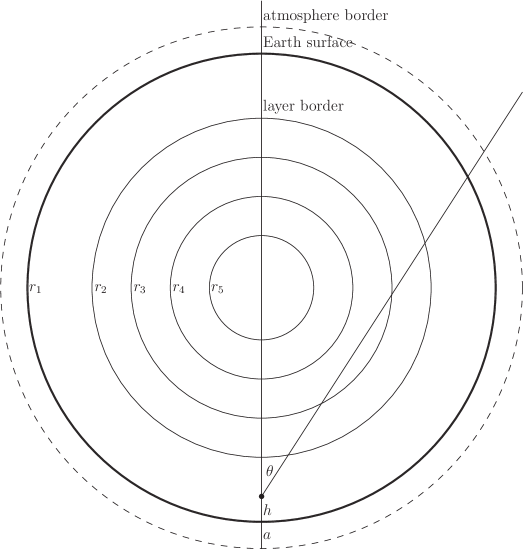
Figure 1: Schematic picture of the Earth structure (not to scale) and definition of the azimuthal angle $\theta$. The detector, marked by black blob, is located at depth $h$ below the Earth surface, the average atmosphere width is denoted by $a$.

The neutrino oscillation probabilities are determined by the $S$-matrix elements ($\alpha,\beta=e,\mu,\tau$):

$$S_{\alpha\beta}=T\ e^{-i\int_{x_{0}}^{x_{f}}{\cal H}(x)dx}$$ (2.1)

with

$${\cal H}=U\left(\begin{array}[]{ccc}0&0&0\\ 0&{\Delta m^{2}_{\odot}\over 2E}&0\\ 0&0&{\Delta m^{2}_{a}\over 2E}\end{array}\right)U^{\dagger}+\left(\begin{array}[]{ccc}V(x)&0&0\\ 0&0&0\\ 0&0&0\end{array}\right)$$ (2.8)

where $U$ denotes the neutrino mixing matrix in the vacuum, with the parametrization:

$$U=O_{23}\,U_{\delta}\,O_{13}\,O_{12}$$ (2.9)

and

$$O_{12} = \left(\begin{array}[]{ccc}\cos\theta_{12}&\sin\theta_{12}&0\\ -\sin\theta_{12}&\cos\theta_{12}&0\\ 0&0&1\end{array}\right)\qquad O_{13}=\left(\begin{array}[]{ccc}\cos\theta_{13}&0&\sin\theta_{13}\\ 0&1&0\\ -\sin\theta_{13}&0&\cos\theta_{13}\end{array}\right)$$ (2.16)

$$O_{23} = \left(\begin{array}[]{ccc}1&0&0\\ 0&\cos\theta_{23}&\sin\theta_{23}\\ 0&-\sin\theta_{23}&\cos\theta_{23}\end{array}\right)\qquad U_{\delta}=\left(\begin{array}[]{ccc}1&0&0\\ 0&1&0\\ 0&0&e^{i\delta}\end{array}\right)$$ (2.23)

The $V(x)$ is the neutrino weak interaction potential energy in matter. As shown in ref. [26], for a constant $V$, to a good approximation the Hamiltonian ${\cal H}$ can be diagonalized by the matrix $U_{m}$ where only the $\theta_{12}$ and $\theta_{13}$ angles have values modified compared to vacuum:

$${\cal H}=U_{m}\left(\begin{array}[]{ccc}{\cal H}_{1}&0&0\\ 0&{\cal H}_{2}&0\\ 0&0&{\cal H}_{3}\end{array}\right)U_{m}^{\dagger} \equiv U_{m}{\cal H}_{d}U_{m}^{\dagger}$$ (2.27)

with

$$U_{m}=O_{23}\,U_{\delta}\,O_{13}^{m}\,O_{12}^{m}$$ (2.28)

and approximate explicit formulae for $O_{13}^{m},O_{12}^{m}$ are given in ref. [26].

It is convenient to work in a new basis, rotated by the matrix

$$U_{0}=O_{23}\,U_{\delta}\,O_{13}$$ (2.29)

so that the rotated Hamiltonian has the form

$${\cal H^{\prime}}\equiv U_{0}^{\dagger}{\cal H}U_{0}=\left(\begin{array}[]{ccc}{\Delta m^{2}_{\odot}\over 2E}s_{12}^{2}&{\Delta m^{2}_{\odot}\over 2E}s_{12}c_{12}&0\\ {\Delta m^{2}_{\odot}\over 2E}s_{12}c_{12}&{\Delta m^{2}_{\odot}\over 2E}c_{12}^{2}&0\\ 0&0&{\Delta m^{2}_{a}\over 2E}\end{array}\right)+V\left(\begin{array}[]{ccc}c_{13}^{2}&0&s_{13}c_{13}\\ 0&0&0\\ s_{13}c_{13}&0&s_{13}^{2}\end{array}\right)$$ (2.36)

and can be approximately diagonalized by $12,13$ rotations only, with angles including matter effects:

$${\cal H}^{\prime}=O_{13}^{T}\,O^{m}_{13}\,O^{m}_{12}{\cal H}_{d}\,O^{mT}_{12}\,O^{mT}_{13}\,O_{13}$$ (2.37)

The transition matrix $S$ can written as the time-ordered product of the transition matrices in the Earth layers,

$$S=T\,\Pi_{i}S_{i}$$ (2.38)

where within the $i$-th layer of constant density the matrix $S_{i}$ is simply given by

$$S_{i}=e^{-i{\cal H}_{i}\Delta x_{i}}$$ (2.39)

Using the rotated basis defined above, one can easily show that (up to an unimportant overall phase denoted as $e^{i\xi}$) the matrix $S$ can be expressed as

$$S=U_{0}\left(T\,\Pi_{i}e^{-i{\cal H}^{\prime}_{i}\Delta x_{i}}\right)U_{0}^{\dagger}=e^{i\xi}U_{a}\,T\,\Pi_{i}\left(O^{m}_{i13}\,O^{m}_{i12}{\cal E}_{i}\,O^{mT}_{i12}\,O^{mT}_{i13}\right)\,U_{a}^{\dagger}$$ (2.40)

where we have defined

$$U_{a} = O_{23}\,U_{\delta}$$

$${\cal E}_{i} = \left(\begin{array}[]{ccc}e^{\frac{1}{2}i({\cal H}^{i}_{2}-{\cal H}^{i}_{1})\Delta x_{i}}&0&0\\ 0&e^{-\frac{1}{2}i({\cal H}^{i}_{2}-{\cal H}^{i}_{1})\Delta x_{i}}&0\\ 0&0&e^{-i({\cal H}^{i}_{3}-\frac{{\cal H}^{i}_{1}+{\cal H}^{i}_{2}}{2})\Delta x_{i}}\end{array}\right)$$ (2.44)

Formula (2.40) is general and does not involve any approximation yet (other than the “layered Earth” model). In the next Section we introduce analytical approximations appropriate for the oscillation probabilities of the sub-GeV atmospheric neutrinos.

3 Analytical approximations for sub-GeV atmospheric neutrinos

3.1 Averaging of probabilities over energy bins

The transition probabilities for sub-GeV atmospheric neutrinos oscillate quickly with neutrino energy and azimuthal angle. This can be traced back to the fact that small variations of both quantities can significantly change the ratio $\Delta m^{2}_{a}L(\theta)/E$. Realistically, the oscillation probabilities have to be averaged over bins in energy and angle corresponding to the relevant experimental resolutions. As long as the period of the neutrino oscillation frequency is far smaller than the experimental resolution significant simplifications can be performed in calculating analytically the averaged oscillation probabilities.

First, we observe that in the product (2.40) the following structure repeats itself:

$$\ldots{\cal E}_{i}\,O^{mT}_{i12}\,O^{mT}_{i13}\,O^{m}_{(i+1)13}\,O^{m}_{(i+1)12}\,{\cal E}_{i+1}\ldots$$ (3.1)

with the most inner multiplication matrix depending on the differences of the $\theta_{13}^{m}$ mixing angle between the neighbouring layers:

$$O^{mT}_{i13}\,O^{m}_{(i+1)13}=\left(\begin{array}[]{ccc}\cos(\theta_{i13}^{m}-\theta_{(i+1)13}^{m})&0&\sin(\theta_{i13}^{m}-\theta_{(i+1)13}^{m})\\ 0&1&0\\ -\sin(\theta_{i13}^{m}-\theta_{(i+1)13}^{m})&0&\cos(\theta_{i13}^{m}-\theta_{(i+1)13}^{m})\end{array}\right)$$ (3.5)

Contrary to high energy neutrinos, like for instance in the Dune experiment [26], for the neutrino energies below $E<{\cal O}(1)$ GeV and typical values of the Earth density, $\theta_{i13}^{m}$ angle in matter vary only very slightly, as illustrated in Fig. 2. The differences $\theta_{i13}^{m}-\theta_{(i+1)13}^{m}$ between the layers are typically of the order of $0.01$ radian, even less for the lower neutrino energies. Therefore, to a good approximation products of $O^{mT}_{i13}\,O^{m}_{(i+1)13}$ can be replaced by the unit matrices. Note, in particular, that for $E<{\cal O}(1)$ GeV and the matter densities in the Earth layers in the range $(3-12)\frac{\mathrm{g}}{\mathrm{cm}^{3}}$ we are well below the resonantly enhanced values of $\theta^{m}_{13}$. In contrast, the dependence of the $\theta_{i12}^{m}$ on the matter density is stronger for this energy range.

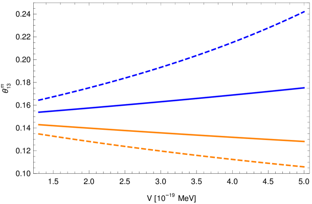
Figure 2: $\theta_{13}^{m}$ in matter as the function of neutrino interaction potential in Earth for normal (blue line) and inverted (orange line) mass ordering and for the neutrino energies $E=400$ MeV (solid lines) and $E=1000$ MeV (dashed lines).

Then, neglecting the overall phase, the time-ordered product on the RHS of eq. (2.40) takes the form

$$O^{m}_{13-first}\,T\,\Pi_{i}\left(O^{m}_{i12}{\cal E}_{i}\,O^{mT}_{i12}\,\right)O^{mT}_{13-last}$$ (3.6)

First layer on the neutrino track is the atmosphere, so that $O^{m}_{13-first}\approx O_{13}$ in vacuum. The last layer is the Earth crust around the detector, so that $O^{m}_{13-last}=O^{m}_{13-crust}$. The inner product in eq. (3.6) contain only $O_{i12}^{m}$ mixing matrices, thus the result has the structure:

$$T\,\Pi_{i}\left(O^{m}_{i12}{\cal E}_{i}\,O^{mT}_{i12}\,\right)=\left(\begin{array}[]{ccc}X_{11}&X_{12}&0\\ X_{12}&X_{22}&0\\ 0&0&0\end{array}\right)+\left(\begin{array}[]{ccc}0&0&0\\ 0&0&0\\ 0&0&\Pi_{i}({\cal E}_{i})_{33}\end{array}\right)$$ (3.13)

Approximating again the product $O^{mT}_{13-crust}O_{13}$ by the unit matrix we arrive at the following expression for the transition matrix $S$ (up to an unimportant overall phase factor):

$$S \approx U_{0}\left(\begin{array}[]{ccc}X_{11}&X_{12}&0\\ X_{12}&X_{22}&0\\ 0&0&0\end{array}\right)U_{0}^{\dagger}+\Pi_{i}({\cal E}_{i})_{33}\,U_{0}\left(\begin{array}[]{ccc}0&0&0\\ 0&0&0\\ 0&0&1\end{array}\right)U_{0}^{\dagger}$$ (3.20)

$$\equiv A+\Pi_{i}({\cal E}_{i})_{33}\,B$$ (3.21)

The matrix $A=A(E,\theta)$ can be calculated by the numerical diagonalization of the Hamiltonian given in eq. (2.8) and the matrix $B$ is constant, given by the vacuum mixing angles. Oscillation probabilities are given by

$$P_{\alpha\beta}=|S_{\beta\alpha}|^{2}=|A_{\beta\alpha}|^{2}+2\mathrm{Re}\left[A^{*}_{\beta\alpha}B_{\beta\alpha}\,\Pi_{i}({\cal E}_{i})_{33}\right]+|B_{\beta\alpha}|^{2}$$ (3.22)

In eq. (3.22) only the quantity $\Pi_{i}({\cal E}_{i})_{33}$ (being a pure phase) depends on the larger neutrino mass splitting and varies quickly with energy and azimuthal angle. When averaged over bins in energy $\Delta E$ and angle $\Delta\theta$ larger than the period of the oscillation frequency, that term vanishes and we get:

$$\bar{P}_{\alpha\beta}(E,\theta) = \frac{1}{\Delta E\Delta\theta}\int_{E-\frac{\Delta E}{2}}^{E+\frac{\Delta E}{2}}\int_{\theta-\frac{\Delta\theta}{2}}^{\theta+\frac{\Delta\theta}{2}}P_{\alpha\beta}(E^{\prime},\theta^{\prime})dE^{\prime}d\theta^{\prime}$$ (3.23)

$$= \frac{1}{\Delta E\Delta\theta}\int_{E-\frac{\Delta E}{2}}^{E+\frac{\Delta E}{2}}\int_{\theta-\frac{\Delta\theta}{2}}^{\theta+\frac{\Delta\theta}{2}}|A_{\beta\alpha}|^{2}dE^{\prime}d\theta^{\prime}+|B_{\beta\alpha}|^{2}$$

This is the first important result of the paper – the averaging over energy and azimuthal angle can be now done using some standard 2-dimensional numerical integration techniques, expected to be quickly converging and accurate as the numerically most difficult and CPU-time consuming averaging over fast oscillations of probabilities has been done analytically while obtaining the formulae  (3.23).

Furthermore, as we show below, one can also derive for the matrix $A$, and thus for the integrand in eq. (3.23), an excellent analytical approximation in terms of only two effective parameters. For neutrino energies larger than $300-400$ MeV, they are very accurately calculable analytically. Clearly, formula (3.23) is useful when typical experimental bins in energy and azimuthal angle are bigger than the period of oscillation frequencies. As discussed in the Appendix B.1 this is true for sub-GeV neutrino energies. For higher energies $E\lower 3.01385pt\hbox{$\;\stackrel{{\scriptstyle\textstyle>}}{{\sim}}\;$}1$ GeV the probabilities defined in eq. (3.23) do not agree well with the formulae (3.22).

3.2 Analytical results for the matrix $A$

We begin with the discussion of the properties of the matrix $X$. The full $2\times 2$ matrix $X$ defined in eq. (3.6) is a time-ordered product of matrices of the form $X_{i}=O^{m}_{i12}{\cal E}_{i}\,O^{mT}_{i12}$ (one for each Earth layer). With the phase conventions chosen in eq. (2.44), each of matrices $X_{i}$ is unitary, symmetric and have determinant equal to 1. Any such matrix has only 2 free real parameters and can be expressed as:

$$X_{i}(\alpha_{i},\phi_{i})=\left(\begin{array}[]{cc}\cos\alpha_{i}\,e^{-i\phi_{i}}&-i\sin\alpha_{i}\\ -i\sin\alpha_{i}&\cos\alpha_{i}\,e^{i\phi_{i}}\end{array}\right)$$ (3.26)

Defining

$$\nu_{i}=({\cal H}^{i}_{2}-{\cal H}^{i}_{1})\Delta x_{i}$$ (3.27)

direct calculations lead to the formulae

$$X_{i}=\left(\begin{array}[]{cc}\cos\frac{\nu_{i}}{2}+i\cos 2\theta_{i12}^{m}\sin\frac{\nu_{i}}{2}&-i\sin 2\theta_{i12}^{m}\sin\frac{\nu_{i}}{2}\\[11.38109pt] -i\sin 2\theta_{i12}^{m}\sin\frac{\nu_{i}}{2}&\cos\frac{\nu_{i}}{2}-i\cos 2\theta_{i12}^{m}\sin\frac{\nu_{i}}{2}\end{array}\right)$$ (3.30)

so that comparing with eq. (3.26) one has

$$\sin\alpha_{i} = \sin 2\theta_{i12}^{m}\,\sin\frac{\nu_{i}}{2}$$

$$\tan\phi_{i} = -\cos 2\theta_{i12}^{m}\tan\frac{\nu_{i}}{2}$$ (3.31)

Let us note that excluding azimuthal angles close to $\pi/2$ or bigger (when the length of the neutrino track in the atmosphere and the asymmetric position of the detector under the Earth surface cannot be neglected) our setup is symmetric with respect to the Earth center. Thus, the full matrix $X$ is to a good approximation given by a symmetric product of $X_{i}$ and has the same symmetry properties as each of them separately:

$$X=X_{1}\ldots X_{k-1}X_{k}X_{k-1}\ldots X_{1}\approx\left(\begin{array}[]{cc}\cos\alpha_{X}e^{-i\phi_{X}}&-i\sin\alpha_{X}\\ -i\sin\alpha_{X}&\cos\alpha_{X}e^{i\phi_{X}}\end{array}\right)$$ (3.34)

The quality of this approximation turns out to be very good, as discussed in Appendix B.2.

Using the parametrization of eq. (3.34), one can derive compact expressions in terms of the effective parameters $\phi_{X},\alpha_{X}$ for the $\nu_{\alpha}\to\nu_{\beta}$ oscillation probabilities given by eq. (3.23):

$$\bar{P}_{\alpha\beta}(E,\theta)=\frac{1}{\Delta E\Delta\theta}\int_{E-\frac{\Delta E}{2}}^{E+\frac{\Delta E}{2}}\int_{\theta-\frac{\Delta\theta}{2}}^{\theta+\frac{\Delta\theta}{2}}I_{\alpha\beta}(E^{\prime},\theta^{\prime})dE^{\prime}d\theta^{\prime}$$ (3.35)

where the matrix elements of $I_{\alpha\beta}$ defined as

$$I_{\alpha\beta}=|A_{\beta\alpha}|^{2}+|B_{\beta\alpha}|^{2}$$ (3.36)

are given by .

$$I_{ee} = \sin^{4}\theta_{13}+\cos^{4}\theta_{13}\cos^{2}\alpha_{X}$$

$$I_{e\mu} = 2\cos^{2}\theta_{13}\sin^{2}\theta_{13}\sin^{2}\theta_{23}+\cos^{2}\theta_{13}(\cos^{2}\theta_{23}-\sin^{2}\theta_{13}\sin^{2}\theta_{23})\sin^{2}\alpha_{X}$$

$$+ \frac{1}{2}\cos^{2}\theta_{13}\sin\theta_{13}\sin 2\theta_{23}\sin 2\alpha_{X}\sin(\delta-\phi_{X})$$

$$I_{\mu e} = 2\cos^{2}\theta_{13}\sin^{2}\theta_{13}\sin^{2}\theta_{23}+\cos^{2}\theta_{13}(\cos^{2}\theta_{23}-\sin^{2}\theta_{13}\sin^{2}\theta_{23})\sin^{2}\alpha_{X}$$

$$- \frac{1}{2}\cos^{2}\theta_{13}\sin\theta_{13}\sin 2\theta_{23}\sin 2\alpha_{X}\sin(\delta+\phi_{X})$$

$$I_{\mu\mu} = \cos^{4}\theta_{13}\sin^{4}\theta_{23}+\cos^{2}\alpha_{X}(\cos^{4}\theta_{23}+\sin\theta_{13}^{4}\sin^{4}\theta_{23}+\frac{1}{2}\cos 2\phi_{X}\sin^{2}\theta_{13}\sin^{2}2\theta_{23})$$ (3.37)

$$+ \sin\theta_{13}(\cos^{2}\theta_{23}-\sin^{2}\theta_{13}\sin^{2}\theta_{23})\sin 2\theta_{23}\sin 2\alpha_{X}\sin\phi_{X}\cos\delta$$

$$+ \sin^{2}\theta_{13}\sin^{2}2\theta_{23}\sin^{2}\alpha_{X}\cos^{2}\delta$$

The same formulae hold for the antineutrino oscillation probabilities, after replacing $\delta\rightarrow-\delta$ and using effective parameters $\bar{\phi}_{X}$, $\sin\bar{\alpha}_{X}$ describing antineutrino mixing (see discussion below and eq. (3.42)).

For narrow energy and azimuthal angle bins one has $\bar{P}_{\alpha\beta}(E,\theta)\approx I_{\alpha\beta}(E,\theta)$. In Sec. 4 we discuss qualitative properties of $\bar{P}_{\alpha\beta}(E,\theta)$ using this approximation, i.e. assuming both quantities to be equivalent. Averaging over wider energy and azimuthal angle bins is discussed in more details in Sec. 5.

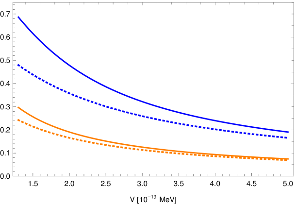
Figure 3: $\sin 2\theta_{12}^{m}$ in the matter for neutrinos (solid lines) and antineutrinos (dashed lines) as the function of their interaction potential with Earth for energy $E=400$ MeV (blue lines) and $E=1000$ MeV (orange lines). Plots for the normal and inverted hierarchy do not differ.

In the next step, one can obtain analytical formulae for the angles $\phi_{X},\alpha_{X}$. We observe that (using the formulae from ref. [26]) in the limit of large $E\,V$ product the quantity $\sin 2\theta_{12}^{m}$ can be expanded as

$$\sin 2\theta_{12}^{m} = \frac{\cos\theta_{13}\sin 2\theta_{12}}{2\cos^{2}2\theta_{13}}\,\frac{\Delta m^{2}_{\odot}}{EV}+{\cal O}\left(\left(\frac{\Delta m^{2}_{\odot}}{EV}\right)^{2}\right)$$ (3.38)

Therefore, for increasing energy $\sin 2\theta_{12}^{m}$ is suppressed approximately by $1/(E\,V)$ factor (as illustrated in Fig. 3). For sufficiently high values of $E$ one can expand the product (3.34) using the expression for $X_{i}$ matrices given by eq. (3.30) and keeping at most the terms linear in $\epsilon_{i}\equiv\sin 2\theta_{12}^{mi}$. Direct multiplication leads then to the remarkably compact formulae

$$\phi_{X} = \nu_{1}+\nu_{2}+\ldots+\frac{1}{2}\nu_{k}$$

$$\sin\alpha_{X} = (\epsilon_{k}-\epsilon_{k-1})\sin\frac{\nu_{k}}{2}+(\epsilon_{k-1}-\epsilon_{k-2})\sin\left(\nu_{k-1}+\frac{\nu_{k}}{2}\right)+\ldots$$ (3.39)

$$+ (\epsilon_{2}-\epsilon_{1})\sin\left(\nu_{2}+\nu_{3}+\ldots+\frac{\nu_{k}}{2}\right)+\epsilon_{1}\sin\left(\nu_{1}+\nu_{2}+\ldots\frac{\nu_{k}}{2}\right)$$

where the quantities $\nu_{i}$ and $\epsilon_{i}$ can be calculated by numerical diagonalization of the neutrino mixing matrices in Earth layers or, to a very good accuracy, using the approximate formulae of ref. [26].

Such an approximation works well even for energy as low as 300 MeV and large values of $\sin 2\theta_{12}^{mi}$. This can be attributed to the fact that the neglected higher order terms in eq. (3.39) are suppressed by additional $\epsilon_{i}^{2}$ factors. Eq. (3.39) reproduces correctly the values of $\alpha_{X}$ and $\phi_{X}$ derived from the numerical calculation of the matrix $A$ (see Appendix B.2) up to about $E=2$ GeV. However, as we have stressed earlier, for energies $E\lower 3.01385pt\hbox{$\;\stackrel{{\scriptstyle\textstyle>}}{{\sim}}\;$}1$ GeV the probabilities defined in eq. (3.23) do not agree well with the formulae (3.22) and the parametrization in terms of $\alpha_{X},\phi_{X}$ is not useful any more.

Eq. (3.39) has some remarkable properties. Firstly, it shows that the overall neutrino oscillation phase is just a direct sum of phases in all layers. In addition, one can check that for neutrino energies in the range $(300-1000)$ MeV the difference between the eigenvalues of the Hamiltonian defined in eq. (2.8) becomes almost constant:

$${\cal H}_{2}-{\cal H}_{1}\approx V\cos^{2}\theta_{13}$$ (3.40)

For $E>300$ MeV energy-dependent corrections to eq. (3.40) are small and the phases $\nu_{i}$ in eq. (3.39) (thus also the overall phase $\phi_{X}$) depend to a good approximation only on the azimuthal angle and the Earth layers density:

$$\nu_{i}\approx V_{i}\cos^{2}\theta_{13}\Delta x_{i}(\theta)$$ (3.41)

where the explicit formulae for the oscillation lengths $\Delta x_{i}(\theta)$ are given in Appendix A.

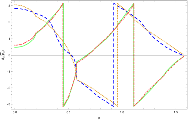
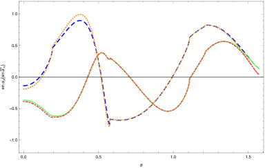
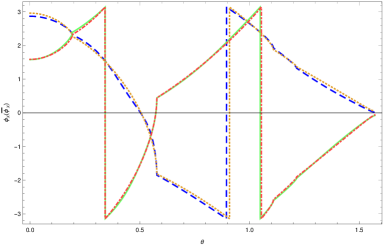
Figure 4: The left panels show comparison of $\phi_{X}$ obtained from numerical diagonalization (blue dashed lines) vs. the approximate formulae of eq. (3.39) (orange dotted lines) and similarly for $\bar{\phi}_{X}$ and eq. (3.42) (green solid and red dot-dashed line, respectively) as a function of the azimuthal angle. The right panels show the analogous comparison of $\sin\alpha_{X}$ and $\sin\bar{\alpha}_{X}$. Chosen neutrino energies are $E=300$ MeV for the upper row and $E=500$ MeV for the lower row. Normal mass ordering is assumed.

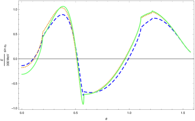
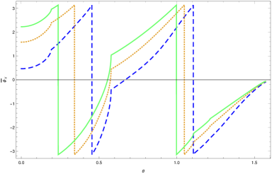
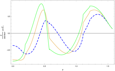
Figure 5: Dependence of $\phi_{X},\bar{\phi}_{X},\frac{E}{300~{}\mathrm{MeV}}\sin\alpha_{X}$ and $\frac{E}{300~{}\mathrm{MeV}}\sin\bar{\alpha}_{X}$ obtained from numerical diagonalization on the azimuthal angle for the neutrino energies $E=300,500$ and $1000$ MeV (blue dashed, orange dotted and green solid line, respectively). Normal mass ordering is assumed.

Secondly, since $\epsilon_{i}\equiv\sin 2\theta_{12}^{mi}\sim 1/E$ and the phases $\nu_{i}$ become energy independent, for $E>300$ MeV to a good approximation one has $\sin\alpha_{X}=f(\theta)/E$, where $f(\theta)$ is some function of the azimuthal angle only.

Similar approximation holds for the antineutrino oscillations, for which one needs to replace $V\to-V$ and $\delta\to-\delta$ in eq. (2.8). In this case effective $\bar{\phi}_{X}$ and $\sin\bar{\alpha}_{X}$ parameters (we denote all variables related to antineutrino oscillations with barred symbols) read as:

$$\bar{\phi}_{X} = \bar{\nu}_{1}+\bar{\nu}_{2}+\ldots+\frac{1}{2}\bar{\nu}_{k}$$

$$\sin\bar{\alpha}_{X} = -(\bar{\epsilon}_{k}-\bar{\epsilon}_{k-1})\sin\frac{\bar{\nu}_{k}}{2}-(\bar{\epsilon}_{k-1}-\bar{\epsilon}_{k-2})\sin\left(\bar{\nu}_{k-1}-\frac{\bar{\nu}_{k}}{2}\right)+\ldots$$ (3.42)

$$- (\bar{\epsilon}_{2}-\bar{\epsilon}_{1})\sin\left(\bar{\nu}_{2}+\bar{\nu}_{3}+\ldots+\frac{\bar{\nu}_{k}}{2}\right)-\epsilon_{1}\sin\left(\bar{\nu}_{1}+\bar{\nu}_{2}+\ldots+\frac{\bar{\nu}_{k}}{2}\right)$$

with

$$\bar{\nu}_{i} = (\bar{\cal H}^{i}_{2}-\bar{\cal H}^{i}_{1})\Delta x_{i}$$

$$\bar{\epsilon}_{i} = \sin 2\bar{\theta}_{12}^{mi}$$ (3.43)

The accuracy of approximation (3.42) is even better than that of eq. (3.39) due to the hierarchy of the expansion parameters, $\bar{\epsilon}_{i}<\epsilon_{i}$ (see Fig. 3).

The dependence of $\phi_{X},\bar{\phi}_{X}$ and $\sin\alpha_{X},\sin\bar{\alpha}_{X}$ on energy and azimuthal angle and the comparison of numerical fitting (see Appendix B.2) and analytical approximate formulae of eqs. (3.39, 3.42) for these parameters is illustrated in Fig. 4 (where the normal neutrino mass ordering is assumed). As can be seen, for $E>300-400$ MeV numerical and analytical results agree very well.

Fig. 5 shows how the effective parameters are modified when neutrino or antineutrino energy changes. As discussed above, the dependence of the $\phi_{X}$ and $\sin\alpha_{X}$ on the angle $\theta$ becomes universal with energy, up to an overall $1/E$ scaling of the $\sin\alpha_{X}$ amplitude. For $\bar{\phi}_{X}$, there remains much stronger energy dependence and the $1/E$ scaling of $\sin\bar{\alpha}_{X}$ is less exact. This is a consequence of the fact that in the sub-GeV range the energy-dependent corrections to the approximation $\bar{\cal H}^{i}_{2}-\bar{\cal H}^{i}_{1}\approx-V_{i}\cos^{2}\theta_{13}$ are significantly larger than for the neutrino case.

The dependence of $\phi_{X},\bar{\phi}_{X}$ and $\sin\alpha_{X},\sin\bar{\alpha}_{X}$ on the azimuthal angle for the inverse mass ordering is almost identical, with small differences of the order of few % appearing only for small values of $\theta$.

3.3 Energy and the angular dependence of the oscillation probabilities

As already mentioned in the previous Section, the dependence of $\phi_{X}$ and $E\,\times\,\sin\alpha_{X}$ (and similarly for antineutrinos) on the azimuthal angle is almost identical for the normal and inverted neutrino mass ordering, thus the problem of the CP-phase determination is not affected by the assumption of the mass hierarchy [31].

Using the parametrization of eq. (3.37), for energies larger than $300-400$ MeV one then obtains very compact expressions for the averaged oscillation probabilities. Experimentally detected numbers of electron and muon neutrinos (antineutrinos) are proportional (taking into account their different atmospheric fluxes $N_{\nu_{\mu}}\approx 2N_{\nu_{e}}$) to quantities defined as

$$I_{e} = I_{ee}+2\;I_{\mu e}$$

$$I_{\mu} = I_{\mu\mu}+\frac{1}{2}\;I_{e\mu}$$ (3.44)

From eqs. (3.37) we see that $I_{ee}$ does not depend on the CP-phase. That fact and, in addition, the difference in the electron and muon neutrino (antineutrino) fluxes, make the observable $I_{e}$ much more efficient than $I_{\mu}$ for measuring the CP phase $\delta$ (and similarly for antineutrinos). The latter quantity has some additional (even) CP phase dependence in $I_{\mu\mu}$ that masks the (odd) dependence on the CP phase of $I_{e\mu}$. Assuming the central values for the measured vacuum mixing angles (and the normal mass ordering), for the transition probabilities we get the simple but very accurate approximation:

$$I_{e} \approx 1.00-0.094\sin^{2}\alpha_{X}-0.143\sin 2\alpha_{X}\sin(\delta+\phi_{X})$$

$$I_{\mu} \approx 0.50+0.011\cos 2\phi_{X}+0.011(1-\cos 2\phi_{X})\sin^{2}\alpha_{X}+0.021\sin^{2}\alpha_{X}\cos^{2}\delta$$ (3.45)

$$+ (0.036\cos\phi_{X}\sin\delta+0.029\sin\phi_{X}\cos\delta)\sin 2\alpha_{X}$$

The same equations are valid for antineutrinos, after replacing $\delta\to-\delta$ and $\phi_{X},\alpha_{X}\to\bar{\phi}_{X},\bar{\alpha}_{X}$.

As an immediate consequence of eq. (3.45) we observe that the variation of $\bar{P}_{e}$ with the CP phase $\delta$ cannot be larger than $\approx 0.30$. Furthermore, the effects of CP violation, which as can be seen, are proportional to $\sin 2\alpha_{X}$, decrease approximately like $1/E$ (as it is discussed earlier, this scaling is less exact for antineutrinos). The CP phase dependence of $I_{\mu}$ is much weaker. Both are shown in Fig. 7 for some optimal values of the azimuthal angle, to be discussed in the next section.

For any given energy $E$ and the azimuthal angle $\theta$ the parameters $\phi_{X},\bar{\phi}_{X},\sin\alpha_{X}$ and $\sin\bar{\alpha}_{X}$ are calculable using either the numerical diagonalization of neutrino Hamiltonian and fitting procedure described in Appendix B.2 or, for sufficiently large $E$, the approximate formulae of eq. (3.39) and they depend only on the assumed Earth density profile. Therefore, as follows from eq. (3.45), one can subtract the theoretically known CP-independent terms from the experimentally measured transition probabilities and obtain directly the constraints on the combination $\delta+\phi_{X}(E,\theta)$ or on the products $\cos\phi_{X}\sin\delta,\sin\phi_{X}\cos\delta$. Performing a fit to many bins in energy and azimuthal angle one can determine the value of phase $\delta$ itself.

4 Optimal observables for the CP-phase detection

4.1 Optimal azimuthal angles

The experimental chances of measuring the CP-phase in $\nu_{\mu}\to\nu_{e}(\bar{\nu}_{\mu}\to\bar{\nu}_{e})$ transitions are best when the coefficients of CP-violating terms are maximal. This happens when the $\sin 2\alpha_{X}(\sin 2\bar{\alpha}_{X}$) reaches maximal or minimal value. In Fig. 6 we plot the dependence of $\sin 2\alpha_{X}(E,\theta)(\sin 2\bar{\alpha}_{X}$) as a function of the azimuthal angle for few chosen values of neutrino energy. As can be seen, independently of the neutrino energy, the extreme values of $\sin 2\alpha_{X}(E,\theta)$ are reached for three values of the azimuthal angle $\theta_{1}=0.12\pi,\theta_{2}=0.18\pi,\theta_{3}=0.39\pi$ and for these three values variations $I_{e},I_{\mu}$ with the phase $\delta$ are maximal and give the best chance for its successful measurement. Extreme values of $\sin 2\bar{\alpha}_{X}$ are more energy dependent, however they can be easily calculated, numerically or analytically from eq. (3.42), for any chosen energy value. Therefore, although in what follows we concentrate on discussing the neutrino oscillations, the results can be in a straightforward way extended to the case of antineutrino mixing, leading to similar conclusions.

In Fig. 7, where we plot the dependence of the quantities $I_{e},I_{\mu}$ for neutrinos on the azimuthal angle for $E=400$ MeV and several values of the phase $\delta$ assuming the normal neutrino mass ordering (corresponding plot for the inverse neutrino mass ordering is almost identical). As already mentioned in the previous section, $I_{e}$ is more sensitive to CP-phase than $I_{\mu}$. We also see that there are also ”the worst” values of the azimuthal angle where the dependence on the CP phase vanishes.

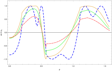
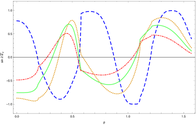
Figure 6: $\sin 2\alpha_{X}$ and $\sin 2\bar{\alpha}_{X}$ plotted as a function of the azimuthal angle varied from 0 to $\pi/2$ for neutrino energies $E=200$ MeV (blue dashed line), $E=400$ MeV (orange dotted line), $E=600$ MeV (green solid line) and $E=1000$ MeV (red dot-dashed line). Normal mass ordering is assumed.

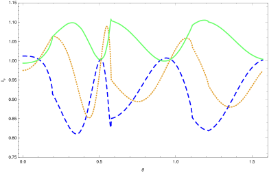
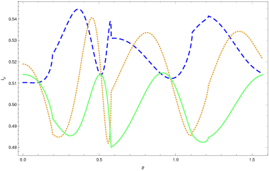
Figure 7: $I_{e}$ (left panel) and $I_{\mu}$ (right panel) for neutrinos as a function of the azimuthal angle varied from 0 to $\pi/2$ and fixed $E=400$ MeV. Blue dashed line: $\delta=0$; orange dotted line: $\delta=\pi/2$; green solid line: $\delta=\pi$. Normal mass ordering is assumed.

For the angles $\theta_{1}$ and $\theta_{3}$, corresponding to maxima of $\sin 2\alpha_{X}$, one has $\phi_{X}(\theta_{1})\approx\phi_{X}(\theta_{3})$ and $\sin\alpha_{X}(\theta_{1})\approx\sin\alpha_{X}(\theta_{3})$. Therefore, measurements done for $\theta_{1}$ and $\theta_{3}$ provide information on $\delta$. For the angle $\theta_{2}$ we get $\sin\alpha_{X}(\theta_{2})\approx-\sin\alpha_{X}(\theta_{1})$ but different phase $\phi_{X}$, thus combining measurements for all three azimuthal angles gives a chance for determining the phase $\delta$ itself. Discussed effects are illustrated in Fig. 8, where we plot the dependence of $I_{e},I_{\mu}$ for neutrinos as a function of the CP-phase for $E=400$ MeV and optimal angles $\theta_{1},\theta_{2},\theta_{3}$. As expected, in this case the variation of $I_{e}$ due to the phase dependence reaches maximal allowed value of $0.30$ and the effect is much weaker for $I_{\mu}$. The maxima and minima of the line corresponding to angle $\theta_{2}$ are shifted compared to other two lines due to different value of $\phi_{X}(\theta_{2})$. For antineutrinos one obtains very similar results, with the optimal values for the azimuthal angle at $E=400$ MeV being $\theta=0.05\pi,0.16\pi,0.29\pi$ and $0.42\pi$.

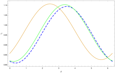
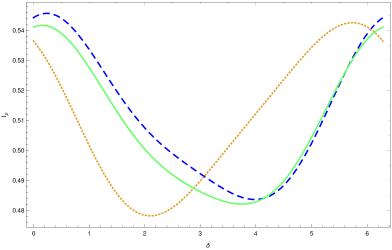
Figure 8: $I_{e}$ (left panel) and $I_{\mu}$ (right panel) for neutrinos as a function of the CP-phase for $E=400$ MeV and optimal angles $\theta_{1},\theta_{2},\theta_{3}$ (blue dashed, orange dotted and green solid line, respectively). Normal mass ordering is assumed.

4.2 Optimised observables

As discussed in the previous Section, eq. (3.37) can be used to determine the phase $\delta$ by subtracting from the experimentally measured transition probability the theoretically calculated CP-independent terms. The analytical understanding of $\phi_{X}$ and $\sin\alpha_{X}$ behaviour has shown that they have very simple energy dependence which allows us to design the alternative observable well suited to measure the CP violating phase, based on subtracting experimentally measured numbers of $\nu_{e}$ and $\nu_{\mu}$, proportional to quantities $I_{e},I_{\mu}$ defined in eq. (3.44) and a well know combination of neutrino vacuum mixing angles. In this case our discussion holds only for the neutrino oscillations, as the energy scaling of antineutrino mixing probability is more complicated and does not allow for such a simple cancellations as we are exploiting below.

Inspection of the expression for $I_{e}$ which can be derived from eq. (3.37) shows that it consists of a constant term depending only on the vacuum oscillation angles, term proportional to $\sin^{2}\alpha_{X}$ but not depending on the phase $\delta$ (which for $E>300-400$ MeV scales to a very good accuracy like $1/E^{2}$) and a term proportional to $\sin(\delta+\phi_{X})$ which scales approximately like $1/E$. Therefore, for $E_{1},E_{2}>300-400$ MeV and for any azimuthal angle $\theta$ the quantity

$$\Delta I_{e}(E_{1},E_{2},\theta) = \frac{E_{1}^{2}}{E_{2}^{2}}I_{e}(E_{1},\theta)-I_{e}(E_{2},\theta)-\left(1-\frac{\sin^{2}2\theta_{13}\cos 2\theta_{23}}{2}\right)\left(\frac{E_{1}^{2}}{E_{2}^{2}}-1\right)$$ (4.1)

$$\approx -\cos^{2}\theta_{13}\sin\theta_{13}\sin 2\theta_{23}\left(\frac{E_{1}^{2}}{E_{2}^{2}}\sin 2\alpha_{X}(E_{1})-\sin 2\alpha_{X}(E_{2})\right)\sin(\delta+\phi_{X})$$

$$\approx -0.14\left(\frac{E_{1}^{2}}{E_{2}^{2}}\sin 2\alpha_{X}(E_{1})-\sin 2\alpha_{X}(E_{2})\right)\sin(\delta+\phi_{X})$$

is to a good approximation proportional solely to the sine of the CP-violating phase shifted by $\phi_{X}$. To maximise $\Delta I_{e}(E_{1},E_{2},\theta)$, one can choose $\theta$ equal or close to the values maximising $|\sin 2\alpha_{X}|$, as described in the previous Section, and large splitting between $E_{1}$ and $E_{2}$, like e.g. $E_{1}=400$ MeV, $E_{2}=1000$ MeV.

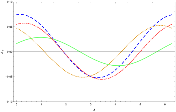
Figure 9: $\Delta I_{e}(E_{1},E_{2},\theta)$ as a function of the phase $\delta$ for $E_{1}=400$ MeV, $E_{2}=1000$ MeV and several chosen values of azimuthal angle: $\theta=0.12\pi$ (blue dashed line), $\theta=0.18\pi$ (orange dotted line), $\theta=0.25\pi$ (green solid line) and $\theta=0.39\pi$ (red dot-dashed line). Normal mass ordering is assumed.

To illustrate the dependence of $\Delta I_{e}(E_{1},E_{2},\theta)$ on the phase $\delta$, in Fig. 9 we plot it for chosen values of energy and azimuthal angles. As expected, the dependence on $\delta$ resembles pure sine function almost symmetric with respect to the horizontal axis.

Achieving similar cancellation of constant term and term proportional to $\sin^{2}\alpha_{X}$ in $I_{\mu}$ is also possible, but requires more theoretical input, as the constant term depends in this case on $\phi_{X}$. Using approximation of eq. (3.39) for $\phi_{X}$, quantity $\Delta I_{\mu}$ defined as

$$\Delta I_{\mu}(E_{1},E_{2},\theta) = \frac{E_{1}^{2}}{E_{2}^{2}}I_{\mu}(E_{1},\theta)-I_{\mu}(E_{2},\theta)-\left(\cos^{4}\theta_{23}+(\cos^{4}\theta_{13}+\sin^{4}\theta_{13})\sin^{4}\theta_{23}\right.$$ (4.2)

$$+ \left.\frac{1}{4}\sin^{2}2\theta_{13}\sin^{2}\theta_{23}+\frac{1}{2}\sin^{2}\theta_{13}\sin^{2}2\theta_{23}\cos 2\phi_{X}\right)\left(\frac{E_{1}^{2}}{E_{2}^{2}}-1\right)$$

can be used to set bounds on different combination of $\sin\delta$ and $\cos\delta$ than the one derived from $\Delta I_{e}$.

5 Measurements with the finite energy and angular resolution

For the neutrino oscillation probabilities one can exploit the simple energy dependence of the effective $\phi_{X},\sin\alpha_{X}$ parameters to simplify expressions for averaging over the finite energy bins. Using the approximate explicit energy scaling properties holding well in the energy range above $300-400$ MeV:

$$\sin\alpha_{X}(E^{\prime},\theta) \approx \frac{E}{E^{\prime}}\sin\alpha_{X}(E,\theta)$$

$$\sin 2\alpha_{X}(E^{\prime},\theta) \approx 2\frac{E}{E^{\prime}}\sin\alpha_{X}(E,\theta)\sqrt{1-\frac{E^{2}}{E^{{}^{\prime}2}}\sin^{2}\alpha_{X}(E,\theta)}$$

$$\phi_{X}(E^{\prime},\theta) \approx \phi_{X}(E,\theta)$$ (5.1)

we can estimate the effect of averaging over hypothetical experimental bins. The integral over energy in eq. (3.35) can be calculated analytically:

$$\frac{1}{\Delta E}\int_{E-\frac{\Delta E}{2}}^{E+\frac{\Delta E}{2}}I_{\alpha\beta}(E^{\prime},\theta^{\prime})dE^{\prime}=I_{\alpha\beta}(E,\theta^{\prime})+{\cal O}\left(\frac{\Delta E^{2}}{E^{2}}\right)$$ (5.2)

For the energy resolutions achievable at Dune [21] or HyperK [22] experiments the term ${\cal O}\left(\frac{\Delta E^{2}}{E^{2}}\right)$ is small and can be neglected. Thus, after integration over the azimuthal angle all averaged transition probabilities $\bar{P}_{\alpha\beta}$ can be expressed in terms of four functions given by the integrals

$$\eta(E,\theta) = \frac{1}{\Delta\theta}\int_{\theta-\frac{\Delta\theta}{2}}^{\theta+\frac{\Delta\theta}{2}}\sin^{2}\alpha_{X}(E,\theta^{\prime})d\theta^{\prime}$$

$$\sigma(E,\theta) = \frac{1}{\Delta\theta}\int_{\theta-\frac{\Delta\theta}{2}}^{\theta+\frac{\Delta\theta}{2}}\cos^{2}\alpha_{X}(E,\theta^{\prime})\cos 2\phi_{X}(\theta^{\prime})d\theta^{\prime}$$

$$\xi_{1}(E,\theta) = \frac{1}{\Delta\theta}\int_{\theta-\frac{\Delta\theta}{2}}^{\theta+\frac{\Delta\theta}{2}}\sin 2\alpha_{X}(E,\theta^{\prime})\cos\phi_{X}(\theta^{\prime})d\theta^{\prime}$$

$$\xi_{2}(E,\theta) = \frac{1}{\Delta\theta}\int_{\theta-\frac{\Delta\theta}{2}}^{\theta+\frac{\Delta\theta}{2}}\sin 2\alpha_{X}(E,\theta^{\prime})\sin\phi_{X}(\theta^{\prime})d\theta^{\prime}$$ (5.3)

E.g., $\bar{P}_{\mu e}$ reads then as

$$\bar{P}_{\mu e} = 2\cos^{2}\theta_{13}\sin^{2}\theta_{13}\sin^{2}\theta_{23}+\cos^{2}\theta_{13}(\cos^{2}\theta_{23}-\sin^{2}\theta_{13}\sin^{2}\theta_{23})\,\eta(E,\theta)$$ (5.4)

$$- \frac{1}{2}\cos^{2}\theta_{13}\sin\theta_{13}\sin 2\theta_{23}\,(\xi_{1}(E,\theta)\sin\delta+\xi_{2}(E,\theta)\cos\delta)$$

Since in the presented formalism $\alpha_{X}$ and $\phi_{X}$ are known as regular functions of the neutrino energy and the azimuthal angle, for any value of $E$ and $\theta$ the coefficients $\eta,\xi_{1},\xi_{2}$ can be easily calculated by simple 1-dimensional numerical integration. Therefore measurements done for different angular momentum bins can provide information on different (but known) combinations of $\sin\delta$ and $\cos\delta$, ultimately giving a good chance to measure the CP-phase itself. Obviously, if necessary one can evaluate them also assuming more complicated Earth structure models including more internal layers, like the full PREM model [29].

The same procedure can be applied to averaging of the quantities $\Delta I_{e},\Delta I_{\mu}$, defined in Sec. 4.2. Up to corrections of the order of ${\cal O}\left(\frac{\Delta E^{2}}{E^{2}}\right)$, the same cancellations between terms as in eq. (4.1) occur for barred probabilities and we can define observable $\Delta\bar{P}_{e}$ averaged over the energy and angular bin as

$$\Delta\bar{P}_{e}(E_{1},E_{2},\theta) = \frac{E_{1}^{2}}{E_{2}^{2}}\bar{P}_{e}(E_{1},\theta)-\bar{P}_{e}(E_{2},\theta)-\left(1-\frac{\sin^{2}2\theta_{13}\cos 2\theta_{23}}{2}\right)\left(\frac{E_{1}^{2}}{E_{2}^{2}}-1\right)$$

$$\approx \frac{1}{\Delta\theta}\int_{\theta-\frac{\Delta\theta}{2}}^{\theta+\frac{\Delta\theta}{2}}\Delta I_{e}(E_{1},E_{2},\theta^{\prime})d\theta^{\prime}$$

$$= -\cos^{2}\theta_{13}\sin\theta_{13}\sin 2\theta_{23}\left(\rho_{1}(E_{1},E_{2},\theta)\sin\delta+\rho_{2}(E_{1},E_{2},\theta)\cos\delta\right)$$

where the functions $\rho_{1}(E_{1},E_{2},\theta),\rho_{2}(E_{1},E_{2},\theta)$ are defined as

$$\rho_{1}(E_{1},E_{2},\theta) = \frac{E_{1}^{2}}{E_{2}^{2}}\xi_{1}(E_{1},\theta)-\xi_{1}(E_{2},\theta)$$

$$\rho_{2}(E_{1},E_{2},\theta) = \frac{E_{1}^{2}}{E_{2}^{2}}\xi_{2}(E_{1},\theta)-\xi_{2}(E_{2},\theta)$$ (5.6)

In a similar manner, $\bar{P}_{\mu}$ can be expressed in terms of $\xi_{1}(E,\theta)$, $\xi_{2}(E,\theta)$ and $\sigma(E,\theta)$. For the antineutrino oscillation probabilities, due to their more complicated energy dependence, averaging of $I_{\alpha\beta}$ over both energy and angle needs to be performed using numerical integration.

6 Summary

We have investigated flavour oscillations of neutrinos and antineutrinos created in the atmosphere by cosmic ray interactions with the air and traversing the Earth. We have focused on sub-GeV neutrinos/antineutrinos ($E<{\cal O}(1)$ GeV) where CP violation effects are large but the oscillation probabilities vary very fast with neutrino energy and its azimuthal angle, far beyond the typical experimental resolution. Therefore, the ”observables”, carrying the physical information, are the averaged probabilities, where the fast oscillation pattern is averaged out. Using the Earth model with layers of constant matter density, we have derived very simple analytic formulae for those averaged probabilities. There are three main formulae summarising our results. Equation (3.23) is the most general expression suitable for fast numerical calculations of the oscillations probabilities averaged over any experimental bins larges than the oscillation periods. Equations (3.35–3.37) give very accurate approximation to the averaged probabilities, where all matter effects are encoded in two effective parameters. And finally, eqs. (3.39,3.41,3.42,3.43) provide for the neutrino/antineutrino energies larger than $300-400$ MeV approximate simple analytical expressions for these effective parameters.

The obtained analytical parametrization is very accurate when compared with the exact numerical calculations. It opens up the possibility of better understanding the dependence of the averaged flavour oscillations of sub-GeV atmospheric neutrinos as a function of their energy and the azimuthal angle with which they hit the detector. In turn, our results can be useful in optimising the experimental measurements of the leptonic CP phase in oscillations of sub-GeV atmospheric neutrinos. We have made several suggestions in that direction, such as the best choice of the azimuthal angles or taking combinations of the data that are directly measuring the CP phase.

Appendix A Oscillation lengths

.

For completeness we include expressions for the length of the neutrino tracks in Earth layers and in the atmosphere. We consider the latter because despite the fact that neutrinos passing through the atmosphere only do not have time to oscillate, they can be important for azimuthal angle $\theta\approx\pi/2$ since they come from full 360 degree plane, while those passing through Earth core come only from the small cone. Thus atmospheric-only neutrinos may produce serious background.

Calculating track lengths is a straightforward exercise in trigonometry. We assume setup defined in Fig. 1, with detector at distance $h$ below Earth surface (it is 1600m for Dune and 650m for HyperK) and atmosphere width denoted by $a$. Obviously $h,a\ll r_{i},R$ thus, in all expressions below we neglect quadratic terms $h^{2},a^{2}$. Let’s consider 3 cases:

1) Neutrino track length in the atmosphere.

$$\Delta x_{atm}=a\,|\cos\theta|\left(1+\frac{2\tan^{2}\theta}{\sqrt{1+\frac{2(a+h)}{R}\tan^{2}\theta}+\sqrt{1+\frac{2h}{R}\tan^{2}\theta}}\right)\qquad 0\leq\theta\leq\pi$$ (A.1)

2) Neutrino track length in the most outer layer (“crust”).

Let’s define $\theta_{li}$ as angles for which neutrino track is tangent to $i$-th layer:

$$\sin\theta_{li}=\frac{r_{i}}{R-h}\qquad\qquad i=1,2,3,4$$ (A.2)

Then for $\theta\geq\theta_{l2}$ neutrino has in 1st layer single undivided track with the length

$$\frac{\Delta x_{1}}{R}=\cos\theta+\sqrt{\cos^{2}\theta+\frac{2h}{R}}-\frac{h}{R}(\cos\theta+|\cos\theta|) \theta\geq\theta_{l2}$$ (A.3)

For $\theta\leq\theta_{l2}$ track has 2 parts, next to detector and on the opposite side of Earth:

$$\frac{\Delta x_{1}^{near}}{R} = \left(1-\frac{h}{R}\right)\cos\theta-\sqrt{\frac{r_{2}^{2}}{R^{2}}-\left(1-\frac{2h}{R}\right)\sin^{2}\theta}$$

$$\frac{\Delta x_{1}^{far}}{R} = \sqrt{\cos^{2}\theta+\frac{2h}{R}\sin^{2}\theta}-\sqrt{\frac{r_{2}^{2}}{R^{2}}-\left(1-\frac{2h}{R}\right)\sin^{2}\theta}$$ (A.4)

3) Neutrino track length in inner layers.

For the more compact notation denote additionally $r_{6}=0$ and $\theta_{l6}=0$. For $i=2,3,4,5$ we get again single track for $\theta_{li}\leq\theta\leq\theta_{l(i+1)}$:

$$\frac{\Delta x_{i}}{R}=2\sqrt{\frac{r_{i}^{2}}{R^{2}}-\left(1-\frac{2h}{R}\right)\sin^{2}\theta}$$ (A.5)

and 2 tracks of identical length for $\theta\geq\theta_{li}$:

$$\frac{\Delta x_{i}^{near}}{R}=\frac{\Delta x_{i}^{far}}{R}=\sqrt{\frac{r_{i}^{2}}{R^{2}}-\left(1-\frac{2h}{R}\right)\sin^{2}\theta}-\sqrt{\frac{r_{i-1}^{2}}{R^{2}}-\left(1-\frac{2h}{R}\right)\sin^{2}\theta}$$ (A.6)

Appendix B Quality of analytical approximations

B.1 Averaged oscillation probability

In order to test the quality of approximation of eq. (3.23), we employ the following procedure.

1. We numerically diagonalize Hamiltonian of eq. (2.8) in each Earth layer and calculate the full transition matrix without any approximations, multiplying layer transition matrices as in eq. (2.38). Resulting transition probability, $P(E,\theta)$ of eq. (3.22), is exact but exhibits fast variations with neutrino energy and with the azimuthal angle.

2. We average $P(E,\theta)$ over energy with the use of numerical integration, using the formula

   $$\hat{P}(E,\theta)=\frac{1}{4\Delta E}\int_{E-2\Delta E}^{E+2\Delta E}P(E^{\prime},\theta)dE^{\prime}$$ (B.1)

   Averaging is done approximately over 4 periods $\Delta E$ of “fast” oscillations in energy, which (in vacuum) are given by

   $$\Delta E=\frac{4\pi E^{2}}{\Delta m_{a}^{2}L(\theta)}$$ (B.2)

   where $L(\theta)$ is the total neutrino track length in Earth for a given azimuthal angle. Actual value of $\Delta E$ in matter differ from the vacuum, but tests show that the result of numerical averaging is stable against variations of $\Delta E$ as long as it has the correct order of magnitude and we integrate over several (here 4) periods $\Delta E$.

3. For each Earth layer we diagonalize numerically Hamiltonian ${\cal H}^{\prime}$ and calculate relevant transition matrix $S_{i}$ in rotated basis of eq. (2.36). We assume the upper $2\times 2$ sub-block of $S_{i}$ to be matrix $X_{i}$, as defined in eq. (3.13). Further, we evaluate full matrix $X$ as a time-ordered product of $X_{i}$ (see eq. (3.34)). Finally, knowing matrix $X$ and hence also the matrices $A,B$ defined in eq. (3.21), we calculate the quantity $I$ (see eq. (3.36)). Finally, for the analytically averaged oscillation probability we use the approximation $\bar{P}(E,\theta)\approx I(E,\theta)$, as discussed in Sec. 4.

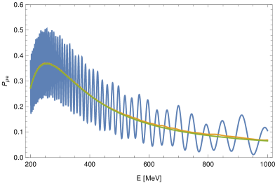
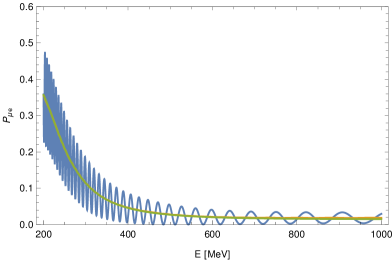
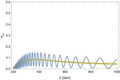
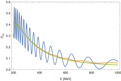
Figure 10: Oscillation probabilities for $\nu_{\mu}\to\nu_{e}$ transitions for the CP-phase $\delta=\pi/2$ as a function of neutrino energy (in MeV) and different azimuthal angles. Blue line: $P_{\mu e}(E,\theta)$, yellow line: $\hat{P}_{\mu e}(E,\theta)$, green line: $\bar{P}_{\mu e}(E,\theta)$. Upper left/right panels: $\theta=\pi/10$ and $\theta=\pi/4$, respectively. Lower left/right panels: $\theta=\pi/3$ and $\theta=\pi/2.5$. Normal mass ordering is assumed.

The comparison of $P$, $\hat{P}$ and $\bar{P}$ is illustrated in Fig. 10. In general, analytical average of eq. (3.23) works very well in the sub-GeV range, some differences between $\bar{P}$ and $\hat{P}$ can be attributed more to the inaccuracies in numerical integration rather then in the approximations used when deriving the formula (3.23).

For the neutrino energies exceeding 1 GeV, the accuracy of approximation (3.23) breaks down, as the variation of probabilities with energy becomes slower and less regular (see Fig. 11). In addition, periods of oscillations may eventually become larger than the experimental resolution in energy and azimuthal angle. Therefore, our analytically averaged formulae for oscillation probabilities should be used only in the sub-GeV neutrino energy range.

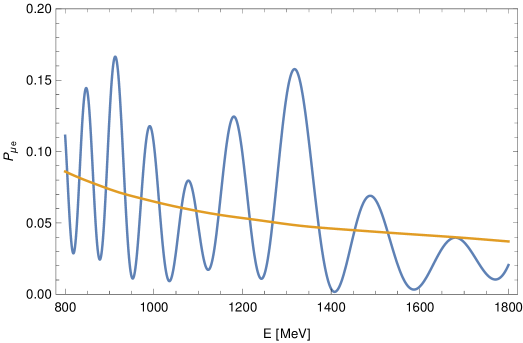
Figure 11: Oscillation probabilities for $\nu_{\mu}\to\nu_{e}$ transitions for the CP-phase $\delta=\pi/2$ as a function of neutrino energy (in MeV) and azimuthal angle $\theta=\pi/10$. Blue line: $P_{\mu e}(E,\theta)$, green line: $\bar{P}_{\mu e}(E,\theta)$. Normal mass ordering is assumed.

B.2 Numerical fits for $\alpha_{X}(\theta,E)$ and $\phi_{X}(\theta,E)$ angles

Matrix $X$ obtained numerically as a $2\times 2$ sub-block of full $3\times 3$ transition matrix (as described in point 3 of the previous Section) is only approximately unitary and symmetric and has determinant slightly different from unity. We obtain best values of angles $\phi_{X},\alpha_{X}$ minimising the difference between the symmetric form on the RHS of eq. (3.26) and the $X$ matrix derived by the numerical diagonalization (denoted below as $X^{num}$), i.e. we seek the minimum of the function

$$f(\alpha,\phi) = |X_{11}^{num}-e^{-i\phi}\cos\alpha|^{2}+|X_{22}^{num}-e^{i\phi}\cos\alpha|^{2}$$ (B.3)

$$+ |X_{12}^{num}+i\sin\alpha|^{2}+|X_{21}^{num}+i\sin\alpha|^{2}$$

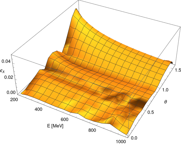
Figure 12: Relative error $\varepsilon_{X}$ of $\alpha_{X},\phi_{X}$ fit plotted as a function of energy varied from 200 to 1000 MeV and azimuthal angle varied from 0 to $\pi/2$.

Minimisation leads to:

$$\phi_{X} = -\arctan\frac{\mathrm{Im}(X_{11}^{num}+(X_{22}^{num})^{*})}{\mathrm{Re}(X_{11}^{num}+(X_{22}^{num})^{*})}$$

$$\alpha_{X} = -\arctan\frac{\mathrm{Im}(X_{12}^{num}+X_{12}^{num})}{|X_{11}^{num}+(X_{22}^{num})^{*}|}$$ (B.4)

Such a procedure reproduces very well $X$ matrix derived by numerical diagonalization. Fig. 12 shows the relative error of a fit as a function of $E$ and $\theta$. The error is defined as

$$\varepsilon_{X}=\frac{||X^{num}-X(\alpha_{X},\phi_{X})||}{||X^{num}||}$$ (B.5)

with $X(\alpha_{X},\phi_{X})$ defined in eq. (3.34).

As one can see, only for low energies $E<400$ MeV and azimuthal angle close to $\pi/2$, where the asymmetry of underground detector position and neutrino track in atmosphere becomes relevant, the error can reach 3-4%. For smaller $\theta$ angles it is always small, confirming the assumed analytical symmetry properties of $X$ matrix and justifying the approximations done in derivation of eq. (3.34).

References

- [1] A. Donini, M. B. Gavela, P. Hernandez, and S. Rigolin, Neutrino mixing and CP-violation, Nucl. Phys. B574 (2000), no. 1-2 23–42, [hep-ph/990].
- [2] T. Ohlsson and H. Snellman, Neutrino oscillations with three flavors in matter: Applications to neutrinos traversing the Earth, Phys. Lett. B 474 (2000) 153–162, [hep-ph/9912295]. [Erratum: Phys.Lett.B 480, 419–419 (2000)].
- [3] Y. Farzan and A. Smirnov, Leptonic unitarity triangle and CP violation, Phys. Rev. D 65 (2002) 113001, [hep-ph/0201105].
- [4] H. Nunokawa, S. J. Parke, and J. W. F. Valle, CP Violation and Neutrino Oscillations, Prog. Part. Nucl. Phys. 60 (2007), no. 02 338–402, [arXiv:0710.0554].
- [5] E. K. Akhmedov, M. Maltoni, and A. Y. Smirnov, Neutrino oscillograms of the Earth: effects of 1-2 mixing and CP-violation, JHEP 06 (2008) 072, [arXiv:0804.1466].
- [6] G. C. Branco, R. Gonzalez Felipe, and F. R. Joaquim, Leptonic CP violation, Rev. Mod. Phys. 84 (2012), no. 2 515, [arXiv:1111.5332].
- [7] T. Ohlsson, H. Zhang, and S. Zhou, Probing the leptonic Dirac CP-violating phase in neutrino oscillation experiments, Phys. Rev. D87 (2013), no. 05 053006, [arXiv:1301.4333].
- [8] S. Razzaque and A. Y. Smirnov, Super-PINGU for measurement of the leptonic CP-phase with atmospheric neutrinos, JEHP 05 (2015) 139, [arXiv:1406.1407].
- [9] P. A. N. Machado, H. Minakata, H. Nunokawa, and R. Zukanovich Funchal, What can we learn about the lepton CP phase in the next 10 years?, JHEP 05 (2014) 109, [arXiv:1307.3248].
- [10] J. Bernabeu and A. Segarra, Disentangling genuine from matter-induced CP violation in neutrino oscillations, Phys. Rev. Lett. 121 (2018), no. 21 211802, [arXiv:1806.07694].
- [11] K. J. Kelly, P. A. N. Machado, I. Martinez-Soler, S. J. Parke, and Y. F. Perez-Gonzalez, Sub-GeV Atmospheric Neutrinos and CP-Violation in DUNE, Phys. Rev. Lett. 123 (2019), no. 08 081801, [arXiv:1904.02751].
- [12] V. Barger, K. Whisnant, S. Pakvasa, and P. R. J. N, Matter effects on three-neutrino oscillations, Phys. Rev. D22 (1980), no. 11 2718.
- [13] A. Ioannisian, DUNE collaboration week, CERN Jan.28-Feb.1, 2019 and DUNE WG meeting, October 2018, indico.fnal.gov/event/18736/contributions/48808/attachments /30464/37472/AraATM.pdf.
- [14] V. Barger, T. J. Weiler, and Whisnant, Generalized Neutrino Mixing from the Atmospheric Anomaly, Phys. Lett. B440 (1998), no. 1-2 1–6, [hep-ph/980].
- [15] O. L. G. Peres and Y. Smirnov A, Atmospheric neutrinos: LMA oscillations, Ue3 induced interference and CP-violation, Nucl. Phys. B680 (2004), no. 1-3 479–509, [hep-ph/030].
- [16] A. Friedland, C. Lunardini, and M. Maltoni, Atmospheric neutrinos as probes of neutrino-matter interactions, Phys. Rev. D70 (2004), no. 11 111301, [hep-ph/040].
- [17] P. Huber, M. Maltoni, and T. Schwetz, Resolving parameter degeneracies in long-baseline experiments by atmospheric neutrino data, Phys. Rev. D71 (2005), no. 05 053006, [hep-ph/050].
- [18] E. A. Hay and D. C. Latimer, Implications of the Dirac CP phase upon parametric resonance for sub-GeV neutrinos, Phys. Rev. D71 (2005), no. 05 053006, [hep-ph/050].
- [19] S. K. Agarwalla, T. Li, O. Mena, and S. Palomares-Ruiz, Exploring the Earth matter effect with atmospheric neutrinos in ice, arXiv:1212.2238.
- [20] M. Blennov and A. Y. Smirnov, Neutrino Propagation in Matter, Adv. High Energy Phys. 2013 (2013) 972485, [arXiv:1306.2903].
- [21] R. Acciarri and el al. [DUNE Collaboration], Long-Baseline Neutrino Facility (LBNF) and Deep Underground Neutrino Experiment (DUNE) Conceptual Design Report Volume 2: The Physics Program for DUNE at LBNF, 1512.06148.
- [22] L. Abe and el al. [Hyper-Kamiokande Proto-Collaboration], Physics Potentials with the Second Hyper-Kamiokande Detectorin Korea, Prog Theor Exp Phys (2018) [arXiv:1611.06118].
- [23] L. Wolfenstein, Neutrino oscillations in matter, Phys. Rev. D17 (1978), no. 9 2369.
- [24] S. P. Mikheev and A. Y. Smirnov, Resonance Amplification of Oscillations in Matter and Spectroscopy of Solar Neutrinos, Sov. J. Nucl. Phys. 42 (1985) 913–917.
- [25] E. K. Akhmedov, Neutrino oscillations in inhomogeneous matter, Sov. J. Nucl. Phys. 47 (1988) 301–302.
- [26] A. Ioannisian and S. Pokorski, Three neutrino oscillations in matter, Phys. Lett. B782 (2018) 641 – 645, [arXiv:1801.10488].
- [27] X. Wang and S. Zhou, Analytical solutions to renormalization-group equations of effective neutrino masses and mixing parameters in matter, JHEP 05 (2019) 035, [arXiv:1901.10882].
- [28] X. Wang and S. Zhou, On the Properties of the Effective Jarlskog Invariant for Three-flavor Neutrino Oscillations in Matter, Nucl. Phys. B 950 (2020) 114867, [arXiv:1908.07304].
- [29] A. M. Dziewonski and D. L. Anderson, Preliminary reference Earth model, Phys. of the Earth and Planetary Interiors 25 (1981), no. 4 297 – 356.
- [30] P. F. de Salas, D. V. Forero, C. A. Ternes, M. Tortola, and J. W. F. Valle, Status of neutrino oscillations 2018: 3 hint for normal mass ordering and improved CP sensitivity, Phys. Lett. B782 (2018) 633–640, [arXiv:1708.01186].
- [31] D. Indumathi, M. Murthy, and L. S. Mohan, Hierarchy independent sensitivity to leptonic with atmospheric neutrinos, Phys. Rev. D 100 (2019), no. 11 115027, [arXiv:1701.08997].