Improved Protein-ligand Binding Affinity Prediction with Structure-Based Deep Fusion Inference: Supplemental Information

Spatial Graph Convolutional Network Architecture

The Spatial Graph Convolutional Neural Network (SG-CNN) presented here is composed of a number of smaller neural networks and can be described in terms of a propagation layer, a gather or aggregation step, and finally, an output fully-connected network. The propagation layer can be understood as the portion of the network where messages are passed between the atoms and used to compute new feature values for each node, with a total of $k_{i}$ rounds of message passing, where $i$ (wlog) corresponds to the ${i^{th}}$ propagation layer.

Using this architecture, we define two distinct propagation layers for covalent and non-covalent interactions. In both cases, we use a single scalar value for the edge feature, the euclidean distance (measured in Angstroms, $\mathrm{\SIUnitSymbolAngstrom}$) between nodes $v_{i}$ and $v_{j}$. Propagation is performed for $k=2$ rounds for both cases, then the attention operation is performed on the final propagation output. For covalent propagation, the input node feature size is 20 and the output size is 16 after the attention operation is applied. For non-covalent propagation, the node features that are the result of the covalent attention operation are used as the initial feature set, the output node feature size of this layer is 12. The resulting features of the non-covalent propagation are then “gathered” across the ligand nodes in the graph to produce a “flattened” vector representation by taking a node-wise summation of the features. This graph summary feature is then fed through the output fully-connected network to produce the binding affinity prediction $\hat{y}$.

$$\forall i~{}h^{k=0}_{i}=x_{i}\qquad\text{for $k=0$}$$ (intialization of node features)

$$h_{i}^{k}=GRU(h_{i}^{k-1},\sum_{j\in\mathcal{N}^{(e)}(v_{i})}f_{e}(h_{j}))\qquad\text{for $k\in\{1...K\}$}$$ (message passing)

where $x_{i}$ is the feature vector of node $v_{i}$.

$$f_{e}(h_{i})=\Theta h_{i}+\sum_{j\in\mathcal{N}(i)}h_{j}\cdot f_{\theta}(e_{i,j})$$ (outer edge network)

where $\Theta$ is a learned set of parameters, $x_{i}$ is the set of features for $n_{i}$, and $f_{\theta}$ is a neural network that computes a new edge feature for the edge $e_{i,j}$ between $v_{i}$ and $v_{j}$.

$$f_{\theta}(e_{i,j})=\phi(f_{\theta_{1}}(\phi(f_{\theta_{2}}(e_{i,j}))))$$ (inner edge network)

where $f_{\theta_{0}}$ and $f_{\theta_{1}}$ are neural networks and $\phi$ is the Softsign (Turian et al. 2009) activation (defined as $1/1+|x|$).

$$h^{K^{\prime}}=\sigma(p(h^{K},h^{k=0}))\odot\big{(}q(b^{K}))$$ (attention operation)

where $\sigma$ is the softmax activation function, $q$ and $p$ are neural networks.

$$h_{gather}=\sum_{v\in G_{ligand}}h_{v}$$ (gather step)

where $G_{ligand}$ is the ligand subgraph of the binding complex graph.

$$\hat{y}=g(h_{gather})=g_{2}(ReLU(g_{1}(ReLU(g_{0}(h_{gather})))))$$ (output network)

Experiment Setup

The 3D-CNN, SG-CNN, and the fusion network models, used an Adam optimizer with learning rate of $1\times 10^{-3}$, $1\times 10^{-3}$, and $1\times 10^{-3}$, respectively. The mini-batch sizes are 50, 8, 100, and the approximate number of epochs are 200, 200, 1000, respectively. We observed that smaller mini-batch sizes drastically improved the model performance in the training of the SG-CNN model while the effect of different mini-batch sizes was negligible in 3D-CNN and the fusion model.

The 3D-CNN and fusion models were developed using the Tensorflow python library (Abadi et al. 2016). The SG-CNN was developed using the PyTorch and PyTorch Geometric (PyG)python libraries (Paszke et al. 2019; Fey and Lenssen 2019) .

Figure 1:

Visualizing Model Bias and MAE distribution

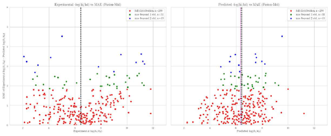
In figure 2 the PDBBind 2016 Core set is color coded into 3 groups according to the MAE of the experimental $log(k_{i}/k_{d})$ (left panel) and the predicted $log(k_{i}/k_{d})$ (right panel). Predictions that fall below one standard deviation of the mean MAE value for a given model (red), between 1-2 standard deviations (green), and exceed 2 standard deviations (blue). Figure 2 shows that models predict over the full range of binding affinity values, however, predictions are biased toward the mean. As the error increases (higher values on the y-axis), the left panel plot shows how high error predictions have trouble predicting the tails of the distribution. The right panel plot shows that the models predict closer to the mean in cases of high error. The black vertical line gives the location of the ground truth mean and the purple vertical line gives the predicted mean.

Figure 2: Scatter plots for each scoring method and the experiment binding affinity measurement.

Relationship between scoring function output with experimental measurement.

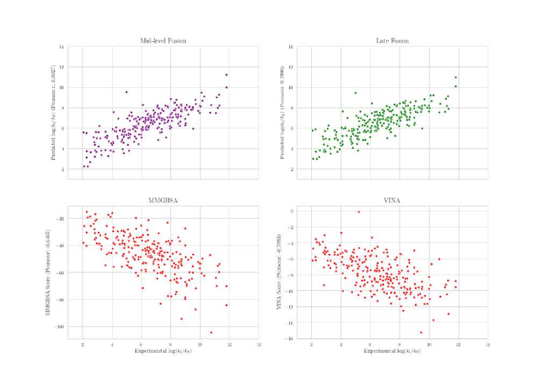
Figure 2 gives scatter plots of the scores from Mid-level Fusion, Late Fusion, MM/GBSA, and Vina scoring methods versus the experimental binding affinity for the 242 complexes of the 2016 core set for which a score across all methods was possible to obtain. Both Fusion methods show a significant improvement over physics-based scoring methods (in terms of Pearson correlation coefficient) with the experimental $log(k_{i}/k_{d})$.

Figure 3: MAE (y-axis) with standard deviation for 57 functional groups (x-axis) defined by CASF-2016. MAE is shown for the machine learning models.

Performance on protein targets (CASF-2016)

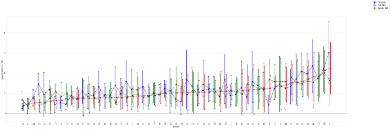
To consider prediction performance of the different models, mean absolute error (MAE) is shown for the 57 functional categories defined by the Comparative Assessment of Scoring Functions (CASF-2016) complexes, which consists of 285 PDBBind core complexes with 5 complexes per category. The results are shown in Figure 3 with the categories sorted on the x-axis by increasing Mid-fusion MAE. The figure shows significantly different Mid-fusion MAE between groups, ranging from approximately 0.5 to over 2 log units. The protein categories are limited by manual curation and were not reported for the complete collection of PDBBind complexes, making it difficult to assess overlap between binding pockets found in the training data and the test set. To address this, a binding pocket oriented structure based clustering scheme was applied to the complete collection of PDBBind complexes.

’

Table 1: Comparison of classifier performance on PDBBind 2016 Core Set - Docking Poses. SD=standard deviation.

Model	Bind ROC AUC	SD	No-bind ROC AUC	SD
SG-CNN	.784	.066	.829	.063
3D-CNN	.747	.081	.774	.063
Vina	.788	.071	.848	.052
MM/GBSA	.828	.064	.833	.057
Late Fusion	.82	.065	.859	.054
Mid-level Fusion	.806	.07	.853	.055

Classification of binders, performance comparison between fusion models and physics-based scoring

For the bind detection screening task, the results are summarized as ROC AUC and reflect randomly partitioning the PDBBind 2016 core set into 5 non-overlapping folds, computing the ROC AUC on each fold, repeating this procedure 100 times and taking the average. The datasets for both tasks maintain a similar class imbalance of 25% positives and 75% negatives. Table 1 show that MM/GBSA has slightly better performance than the Fusion model and both methods show a small improvement (0.04) over Vina. For the no-bind task, while the Fusion model had the highest ROC AUC the margin of difference was negligible compared to Vina (0.011).

Figure 4: Histogram counting minimum Tanimoto distance between each compound in test and nearest match in PDBBind 20016 refined.

Structure similarity between refined abd core sets of PDBBind 2016

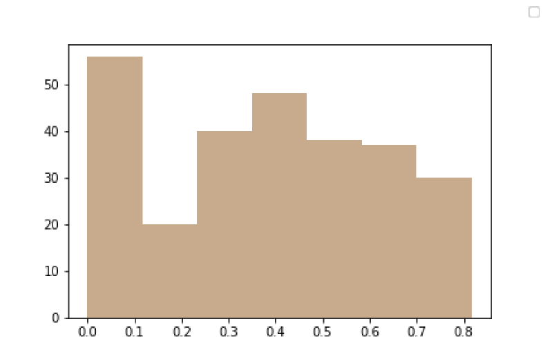
In order to gain an understanding of how “similar” our training set (in terms of the refined set) was to our testing set (the core set), we consider structural similarity between the ligands in the refined and core sets as measure by the tanimoto distance metric. Figure 4 illustrates the distribution of the tanimoto distance between each ligand in the core set with its nearest neighbor in the refined set.

Disclaimer

This document was prepared as an account of work sponsored by an agency of the United States government. Neither the United States government nor Lawrence Livermore National Security, LLC, nor any of their employees makes any warranty, expressed or implied, or assumes any legal liability or responsibility for the accuracy, completeness, or usefulness of any information, apparatus, product, or process disclosed, or represents that its use would not infringe privately owned rights. Reference herein to any specific commercial product, process, or service by trade name, trademark, manufacturer, or otherwise does not necessarily constitute or imply its endorsement, recommendation, or favoring by the United States government or Lawrence Livermore National Security, LLC. The views and opinions of authors expressed herein do not necessarily state or reflect those of the United States government or Lawrence Livermore National Security, LLC, and shall not be used for advertising or product endorsement purposes.

References

- Abadi et al. (2016) Abadi, M. et al. (2016). Tensorflow: A system for large-scale machine learning. In Proceedings of the 12th USENIX Conference on Operating Systems Design and Implementation, OSDI’16, page 265–283, USA. USENIX Association.
- Fey and Lenssen (2019) Fey, M. and Lenssen, J. E. (2019). Fast graph representation learning with pytorch geometric.
- Paszke et al. (2019) Paszke, A. et al. (2019). Pytorch: An imperative style, high-performance deep learning library. In Advances in Neural Information Processing Systems 32, pages 8024–8035. Curran Associates, Inc.
- Turian et al. (2009) Turian, J. et al. (2009). Quadratic features and deep architectures for chunking. In Proceedings of Human Language Technologies: The 2009 Annual Conference of the North American Chapter of the Association for Computational Linguistics, Companion Volume: Short Papers, pages 245–248.