Appendix: How to Close Sim-Real Gap? Transfer in Segmentation!

Design of the imitation expert

We train our DNN controller in simulation, using Gazebo [Koe04] to simulate a Baxter robot. The robot arm is controlled in position mode; we indicate with $[s_{0},s_{1},e_{0},e_{1},w_{0},w_{1},w_{2}]$ the seven joint angles of the robot arm and with $[g_{0}]$ the binary command to open or close the gripper. Controller learning is supervised by an expert that, at each time step, observes joint angles and gripper state, as well as the position of the target sphere. The expert implements a simple but effective finite-state machine policy to grasp the sphere. In state $s_{0}$, the end-effector moves along a linear path to a point $6$cm above the sphere; in state $s_{1}$, the end-effector moves downward to the sphere; when the sphere center is within $0.1$cm from the gripper center, the expert enters state $s_{2}$ and closes the gripper. In case the gripper accidentally hits the sphere or fails to grasp it (this can happen because of simulation noise or control inaccuracies), the expert goes back to $s_{0}$ or $s_{1}$ depending on the new sphere position.

Compared to a more elementary implementation of the expert directly aiming at the sphere, this expert is capable of grasping the sphere with a 96%?? success rate (while the elementary expert achieves approximately 50%). Failures are mostly associated with noise in simulation or inaccurate physics (we noticed that sometimes the sphere jumps away from the gripper abruptly when hit by it). This highlights the important of designing a proper expert for imitation learning - a policy which is ideal in theory may lead to sub-optimal results in simulation and subsequently invalidate the imitation learning procedure.

Image data generation

To collect training data for the vision module, we need to have images as similar to real images as possible, while having cheap annotation of segmentation masks. We can obtain segmentation masks easily from Gazebo images. We can implement a color filter in HSV space that extracts all yellow pixels. However, as shown in insets of Fig. LABEL:fig:teaser, the Gazebo images are noise-free and well lit, shadows are poorly modeled especially when the end-effector is close to the sphere. They are significantly different from real images, thus directly training on these images will not generalize to real environments.

To make the images more realistic, we setup a scene in Povray [povray] with the same table, sphere, and camera arrangements as in Gazebo. Rendered images in Povray have much more realistic lighting, and segmentation masks can be directly rendered. We also approximate the gripper plates with two thin boxes to simulate shadows on the sphere. A sample of rendered image is shown in Fig. LABEL:fig:compose.

Inspired by domain randomization [Jam17, Tob17], to make the training images diverse, including various backgrounds and clutter objects, and at the same time more realistic, we alpha-blend rendered image patches of the sphere with random background images taken by the real robot camera. Fig. LABEL:fig:compose demonstrates the composition process. We rendered $5000$ images of the sphere with random lighting condition and camera position, and collected $1600$ images of the real environment by setting the robot’s arm at random poses in the robot’s workspace. Random objects are placed in the robot workspace as clutter. The collection procedure is completely automated and takes less than an hour. During training, the composed images are randomly shifted in the HSV space to account for the differences in lighting, camera exposure, and color balance.

Close-loop controller learns to recover from failures

In fact, imitation learning using only expert demonstrations may fail to capture such rare behavior, since the expert mostly succeeds at the first attempt and thus the training dataset would rarely include recovery behavior. On the other hand, when training with DAGGER, at iteration $n$ the DNN controller executes the sub-optimal policy $\pi_{n}$ to collect new training data, so it can expose and learn to correct its own errors by querying the expert agent for advice. As a result, the training data covers a larger state distribution than the distribution induced by expert demonstrations, and the trained agent effectively learns to recover from possible failures.

Comparisons with end-to-end approach

Our two-module network can be trained separately or end-to-end. In the main paper we have reported the results while training the two modules separately. In this section we report the results training the network end-to-end, and compare with variants of our network similar to the ones used in  [Dev17, Sin17].

We have made several modifications to the training process in order to make end-to-end training possible. First, at every time step, we copy the position of the end-effector camera and the sphere from Gazebo to Povray, and render an image to compose with a random background. While training the vision module independently, we can simply randomize the camera position to generate image-mask pairs, here we also need to make sure the produced image and segmentation mask matches the expert’s joint commands. Second, since a rendering is required at every time step to replace the Gazebo image, we pause the physics simulation while rendering, in order the keep the command frequency the same as at test time. Last but not the least, we changed the number of training epoch from $200$ for every DAGGER iteration to $250/i$ for the $i$th iteration, so that training time grows linearly with respect to the number of iterations, instead of quadratically. This reduced the end-to-end training time from estimated $134$ days to actually taking $7$ days on a single Titan X GPU.

In comparison, because the network is much smaller, training the controller module alone takes $12$ hours before modification, and can be reduced to $2$ hours after the modification without sacrificing performance. Training the vision module alone requires $1$ hour to collect the real background images, less than $1$ hour to render images with Povray paralleled over 4 threads, and $9$ hours to train the network. Because the vision module is supervised pixel-wise, each image is equivalent to $100\times 100$ training samples, although strongly correlated. The network requires much less updates than the controller network to converge.

When testing on the real robot, The robot executes smoother trajectories, making less attempts before a successful one, and achieves $88\%$ success when no clutter objects present, following the evaluation process described in Sec. LABEL:subsec:vision. When clutter objects are present, the end-to-end trained network shows significant improvement in robustness, and accurately reaches the sphere in all $5$ trials, grasping the sphere in $4$ of them.

We also compare our method to two variants of our network. In the first variant, we keep the network structure unaltered, but do not give supervision to the segmentation layer, thus making it an unsupervised feature map. In the second variant, we increase the feature map from $1$ channel to $32$ channels and calculate the spatial softmax before concatenating with the robot joint angles and feeding to fully connected layers, similar to the networks used in  [Dev17, Sin17]. No supervision is given to the spatial softmax coordinates or the feature maps. Training is otherwise the same with our own network.

We plot the training losses in Fig 1. Our modular network with additional segmentation supervision achieves significantly lower loss than the two variants. When testing on the real robot, our modular network can achieve $88\%$ success rate while the other two variants can drive the robot end-effector near the sphere, but are not accurate enough to grasp the sphere. Arguably this is not a completely fair comparison since addition supervision is used to train our modular network. However we want to demonstrate that by having a well-defined internal state representation as the interface between modules, it is possible to exploit the free annotations available in robotic simulators or graphics engines, and to train autonomous robots more efficiently and effectively.

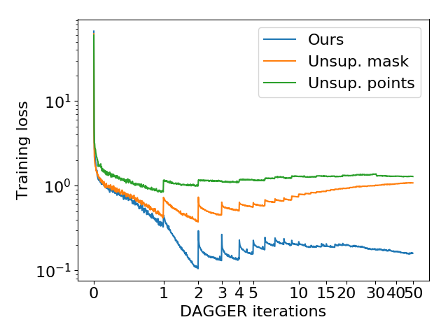
Figure 1: Training loss for end-to-end training of several network variants. Ours (blue line) refers to our proposed network, with both expert action and segmentation supervision, and Povray + real background composed images as input. Unsupervised mask (orange line) refers to the same network and input images, but trained with only the expert action supervision, no segmentation supervision. Unsupervised points (green line) refers to network with spatial softmax on $32$ feature maps. The same input and expert action supervision is provided.