Nonreciprocity as a generic route to traveling states

Abstract

We examine a non-reciprocally coupled dynamical model of a mixture of two diffusing species. We demonstrate that nonreciprocity, which is encoded in the model via antagonistic cross diffusivities, provides a generic mechanism for the emergence of traveling patterns in purely diffusive systems with conservative dynamics. In the absence of non-reciprocity, the binary fluid mixture undergoes a phase transition from a homogeneous mixed state to a demixed state with spatially separated regions rich in one of the two components. Above a critical value of the parameter tuning non-reciprocity, the static demixed pattern acquires a finite velocity, resulting in a state that breaks both spatial and time translational symmetry, as well as the reflection parity of the static pattern. We elucidate the generic nature of the transition to traveling patterns using a minimal model that can be studied analytically. Our work has direct relevance to nonequilibrium assembly in mixtures of chemically interacting colloids that are known to exhibit non-reciprocal effective interactions, as well as to mixtures of active and passive agents where traveling states of the type predicted here have been observed in simulations. It also provides insight on transitions to traveling and oscillatory states seen in a broad range of nonreciprocal systems with non-conservative dynamics, from reaction-diffusion and prey-predators models to multispecies mixtures of microorganisms with antagonistic interactions.

Traveling patterns occur ubiquitously in nature. Examples range from oscillating chemical reactions Field and Burger (1985); Weiss and Deegan (2017); Semenov et al. (2016), waves of metabolic synchronization in yeast Schütze et al. (2011), to the spatial spread of epidemics Diekmann (1978, 1979); Abramson (2003); Wang et al. (2013). Most mathematical models that capture such spatio-temporal dynamics, including reaction-diffusion equations Field and Burger (1985); Erneux and Nicolis (1993); Krischer and Mikhailov (1994); Kondo and Miura (2010); Gambino et al. (2013), excitable systems Keener (1980); Holden et al. (2013), collections of coupled oscillators Hong and Strogatz (2011, 2012), and prey-predator equations Tsyganov et al. (2003); Biktashev and Tsyganov (2009); Mobilia et al. (2007) are unified by the fact that the dynamical variables are non-conserved fields Coullet et al. (1989). In this case the coupling to birth-death or to other reaction processes provides a promoter-inhibitor mechanism that sets up oscillatory states. In this paper we demonstrate that traveling patterns can arise in multi-component systems described by purely diffusive conserved fields from non-reciprocal interactions between species. The appearance of traveling or sustained oscillatory states in a purely diffusive system with no apparent external forcing is unexpected and defies intuition. Our work suggests that non-reciprocity provides a generic mechanism for the establishment of traveling states in the dynamics of conserved scalar fields.

The third law of Newtonian mechanics establishes that interactions are reciprocal: for every action there is an equal and opposite reaction. While of course this remains true at the microscopic level, non-reciprocal effective interactions can occur ubiquitously on mesoscopic scales when interactions are mediated by a nonequilibrium environment Ivlev et al. (2015); Durve et al. (2018); Hayashi and ichi Sasa (2006); Paoluzzi et al. (2018, 2020). A striking physical example is realized in diffusiophoretic colloidal mixtures Soto and Golestanian (2014); Agudo-Canalejo and Golestanian (2019); Saha et al. (2019). Non-reciprocal interactions are also the norm in the living world. Examples are promoter-inhibitor interactions among different cell types Theveneau et al. (2013) and the antagonistic interactions among species in bacterial suspensions Pigolotti and Benzi (2014); Long and Azam (2001); Xiong et al. (2020); Yanni et al. (2019); Curatolo et al. (2019). Social forces that control the behavior of human crowds Helbing and Molnár (1995); Helbing et al. (2000); Bain and Bartolo (2019) and collective animal behavior Strandburg-Peshkin et al. (2013); Vicsek and Zafeiris (2012) are other important examples as well.

To highlight the role of non-reciprocal couplings in driving time-dependent phases, we examine a minimal model of the dynamics of two interdiffusing species, each described by a scalar field $\phi_{\mu}$, for $\mu=A,B$. The evolution of each concentration field is governed by a $\phi^{4}$ field theory that allows for a spinodal instability according to Model B dynamics  Hohenberg and Halperin (1977). When decoupled, each phase field can undergo a Hopf bifurcation describing the transition from a homogeneous state to a phase-separated state composed of dilute and dense phases. The two fields are coupled via cross-diffusion terms with diffusivities $\kappa_{\mu\nu}$. When these couplings are reciprocal, the interaction between the two fields leads to a transition between a mixed state where both fields are homogeneous to a demixed state with distinct regions of high $A$ and low $B$. Non-reciprocity is introduced by allowing the two cross-diffusivities to have opposite signs and is quantified by $\delta=(\kappa_{BA}-\kappa_{AB})/2$. Non-reciprocal cross-diffusivities drive a second transition through a drift bifurcation to a time-dependent state that breaks parity, where the domains of the demixed regions travel at a constant drift velocity. This transition is closely related to ones previously reported in specific models of prey-predator and reaction-diffusion dynamics Fauve et al. (1991); Erneux and Nicolis (1993); Krischer and Mikhailov (1994); Tsyganov et al. (2003); Biktashev and Tsyganov (2009); Kondo and Miura (2010); Wang et al. (2013), but occurs here from the coupling of two conserved fields. We demonstrate that the transition to traveling states is a parity and time-reversal (PT) symmetry breaking bifurcation that arises generically from non-reciprocal couplings. The phase diagram obtained from numerical solutions of a one-dimensional realization of this minimal model in the simplest case where only field A is supercritical, while B is subcritical, i.e., the ground state value of field B is simply $\phi_{B}^{g}=0$, is shown in Fig. 1a. Tuning the control parameter that drives phase separation of species $A$ ($\chi_{A}$) and the measure of non-reciprocity $\delta$, we observe three distinct states: a mixed state where both fields are homogeneous, a static demixed state that breaks translational symmetry with out-of-phase spatial modulations of the two fields, and a time-dependent state that additionally breaks reflection and time-reversal symmetry, where the spatial modulation of the demixed state travels at constant velocity. The solid lines are obtained from a one-mode approximation to the continuum model that can be solved analytically and provides an excellent fit to the numerics. Within this one-mode approximation, the transition from the stationary to the traveling state can be understood as an instability of the relative phase of the first Fourier harmonic of the fields. The instability arises because non-reciprocity allows perturbations in the two fields to travel in the same direction, promoting a “run-and-catch” scenario that stabilizes the traveling pattern. While the spatial pattern in the static demixed phase is even in the relative displacement of the two phase fields, non-reciprocity breaks this reflection symmetry in the traveling state, mediating a PT-symmetry-breaking transition. Note that the transition to a PT-broken phase occurs at finite value of $\delta$, hence requires sufficiently strong non-reciprocity. Finally, the phase boundary separating the static and traveling patterns in Fig. 1a corresponds to a so-called “exceptional point” where the eigenmodes of the matrix controlling the dynamical stability of the system coalesce Kato (1966); Bender (2007); Fruchart et al. (2020). In parallel to our investigation, Saha et al. Saha et al. (2020) have also reported traveling density waves in scalar fields with Cahn-Hilliard dynamics and non-reciprocal couplings. The simulations carried out by these authors support our finding that non-reciprocal couplings provide a generic mechanism for breaking time-reversal symmetry and setting spatial patterns in motion.

A microscopic model that displays the phenomenology captured by Fig. 1a is a mixture of active and passive Brownian particles, where the active component exhibits motility-induced phase separation and fluctuations in the density of passive particles can enhance fluctuations in the density of the active fraction via an effective negative cross diffusivity Wysocki et al. (2016); Wittkowski et al. (2017); Agrawal et al. (2017). The connection between the active-passive mixture and the dynamics embodied by our model is unfolded in the SI. Another realization of this macrodynamics is a binary suspension of colloidal particles where species A attracts species B, but species B repels species A. Such competing interactions have been studied in simple models Yllanes et al. (2017); Bonilla and Trenado (2019) and can be realized in mixtures of self-catalytic active colloids, where the local chemistry mediates non-reciprocal interactions among the two species, as demonstrated for instance in Saha et al. (2019); Agudo-Canalejo and Golestanian (2019) via numerical simulations.

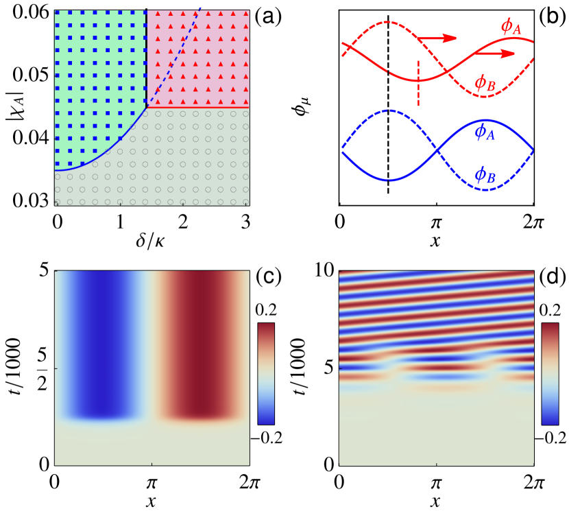
Figure 1: (a) State diagram spanned by $\delta/\kappa$ and $\chi_{A}$. The system has three distinct states: homogeneous (gray, circles), static patterns or demixed (cyan, rectangles), and traveling patterns (pink, triangles). Symbols indicate results from the simulations, while the lines marking the boundaries of the colored domains are obtained from the stability analysis of the one-mode model. The static demixed state exists in the region between the black and the dashed blue lines, but is unstable. (b) Examples of spatial variations of $\phi_{A}(x)$ (solid lines) and $\phi_{B}(x)$ (dashed lines) in the static (blue) and traveling states (red). (c–d) Spatiotemporal patterns of $\phi_{A}(x,t)$ in the (c) static and (d) traveling states. In (b–d), we use $\chi_{A}=-0.05$ and (c) $\delta=\kappa$ and (d) $\delta=2\kappa$.

I Continuum model

We consider a binary mixture described by two conserved phase fields $\phi_{A}$ and $\phi_{B}$ with Cahn-Hillard dynamics Cahn and Hilliard (1958); Elliott (1989); Khain and Sander (2008) augmented by cross-diffusion ,

$$\partial_{t}\phi_{\mu}=\bm{\nabla}\cdot\left[\left(\chi_{\mu}+\phi_{\mu}^{2}-\gamma_{\mu}\nabla^{2}\right)\bm{\nabla}\phi_{\mu}+\kappa_{\mu\nu}\bm{\nabla}\phi_{\nu})\right]\;,$$ (1)

where $\mu,\nu=A,B$ and no summation is intended. In the absence of cross-diffusive couplings ($\kappa_{\mu\nu}=0$), the fields are decoupled, with ground states $\phi_{\mu}^{g}=0$ for $\chi_{\mu}>0$, describing homogeneous states, and $\phi_{\mu}^{g}=\pm\sqrt{-3\chi_{\mu}}$ when $\chi_{\mu}<0$, corresponding to phase separated states.

The cross-diffusivities control interspecies interaction, allowing phase gradient of one species to drive currents of the other species. Equal cross-diffusivities, $\kappa_{AB}=\kappa_{BA}=\kappa$, yield an effective repulsion between the two fields. When sufficiently strong to overcome the entropy of mixing, such a repulsion results in the formation of spatial domains of high/low $\phi_{A}/\phi_{B}$, i.e., a demixed state. Here, in contrast, we introduce non-reciprocity by allowing these two quantities to have opposite signs , as can for instance be achieved in mixtures of active and passive Brownian particles (see SI section VI.B) or in mixtures of colloids with competing repulsive and attractive interactions (see SI section VI.A). We tune the degree of non-reciprocity $\delta>0$ by letting

$$\kappa_{AB}= \kappa-\delta\;,$$

$$\kappa_{BA}= \kappa+\delta\;.$$ (2)

As shown below, this non-reciprocity breaks PT symmetry and gives rise to spatiotemporal patterns of $\phi_{A}$ and $\phi_{B}$ that break both spatial and temporal translation symmetry.

We have studied numerically (1) in a one-dimensional box of length $L=2\pi$, for the case where $\chi_{A}<0$, $\chi_{B}>0$, and ignoring $\phi_{B}^{2}$ in the self-diffusivity. The results are easily generalized to the case where both components are supercritical ($\chi_{A}<0$ and $\chi_{B}<0$) and to higher dimensions (see SI sections IV-V), but remain qualitatively unchanged. We have integrated  (1) with a fourth-order central difference on a uniform grid with spacing $h=2\pi/64$. To march in time, we use a second-order, 128-stage Runge-Kutta-Chebyshev scheme with a time step $\Delta t=0.1$ Hundsdorfer and Verwer (2003); Verwer et al. (1990). All simulations start from nearly uniform phase fields, where weak random fluctuations are added on top of the initial compositions $\phi_{A}^{0}=0$ and $\phi_{B}^{0}=0$. We fix the values of the parameters as: $\gamma_{A}=0.04$, $\gamma_{B}=0$, $\chi_{B}=0.005$, $\kappa=0.005$, and study how the system dynamics changes with $\chi_{A}$ and $\delta$.

We find three distinct states by varying $\chi_{A}$ and $\delta$, as summarized in Fig. 1a. When the cross-diffusivities are reciprocal ($\delta=0$), by increasing $|\chi_{A}|$ the system undergoes a Hopft bifurcation from a homogeneous state (gray circles) to a demixed state (blue rectangles) where the two fields are spatially modulated with alternating regions of high $\phi_{A}$/low $\phi_{B}$ (Figs. 1b,c). This state is stabilized by the cubic term in (1), as in conventional Cahn-Hillard models. Above a critical value of $\delta$, the demixed state undergoes a second bifurcation to a state where the domains of high $\phi_{A}$/low $\phi_{B}$ travel at a constant speed (red triangles in Fig. 1a, see also Figs. 1b, 1d for spatiotemporal patterns). The velocity of the traveling pattern provides an order parameter for this transition, and the direction of motion is picked spontaneously. The opposite signs of the cross-diffusivities provide effective antagonistic repulsive and attractive interactions between the two fields. The drift bifurcation is triggered by the nucleation of a phase shift in the spatial modulation of the two fields that allows species $A$ to outrun $B$, while $B$ tries to catch up with $A$. At weak non-reciprocity, species $A$ is too slow to escape from $B$, and the static pattern is restored. Strong non-reciprocity, on other hand, allows species $A$ to outrun $B$. As the distance between the two increases, $A$ gradually slows down while $B$ speeds up until the two share a common speed and become trapped in a steady traveling state. This “run-and-catch” scenario is quantified below with a simple one-mode analysis of our dynamical equations that captures the behavior quantitatively. The transitions between the various states obtained from the one-mode approximation are shown as solid lines in Fig. 1a and provide an excellent fit to the numerics in one dimension. Finally, as discussed further below, the transition is associated with the breaking of reflection symmetry or parity of the spatial modulations, as well as of time-reversal symmetry, hence provides a realization of a PT-breaking transition.

We show in the SI that the same scenario applies qualitatively in two dimensions. In this case, in addition to traveling spatial structures, we also observe oscillatory patterns that are absent in 1D. In the oscillatory state the system organizes into high/low concentration region of each species that periodically split and merge. The frequency of oscillation increases with $\delta$, suggesting that the oscillating states are a richer manifestation of non-reciprocity and of the “run-an-catch” mechanism that controls the dynamics in 1D. Both traveling and oscillatory states appear to be stable and coexist at high $\delta$, with the state selection being controlled by initial conditions. This suggests that it would be interesting to go beyond the deterministic model considered here to examine the role of noise. A full study of 2D systems will be reported elsewhere.

II One-mode approximation

To uncover the physics behind the PT-breaking bifurcation, we expand the fields $\phi_{\mu}$ in a Fourier series as $\phi_{\mu}(x,t)=\sum_{j=-\infty}^{\infty}\hat{\phi}_{\mu}^{j}(t)e^{iq_{j}x}$, where $\hat{\phi}_{\mu}^{j}=(2\pi)^{-1}\int_{0}^{2\pi}dx\phi_{\mu}e^{-iq_{j}x}$ is the amplitude of mode $j$. Substituting this in (1), and apply the Galerkin method  Hesthaven et al. (2007), one obtains a set of coupled ordinary differential equations for the Fourier amplitudes. For the one dimensional model described above, we have verified numerically that only the first Fourier mode $q_{1}=1$ is activated. We can then replace the original partial differential equations with a single-mode approximation, given by

$$\frac{d\hat{\phi}_{A}^{1}}{dt}= -\left(\alpha_{A}+|\hat{\phi}_{A}^{1}|^{2}\right)\hat{\phi}_{A}^{1}-(\kappa-\delta)\hat{\phi}_{B}^{1},$$ (3a)

$$\frac{d\hat{\phi}_{B}^{1}}{dt}= -\alpha_{B}\hat{\phi}_{B}^{1}-(\kappa+\delta)\hat{\phi}_{A}^{1},$$ (3b)

where $\alpha_{A}=\chi_{A}+\gamma_{A}+(\phi_{A}^{0})^{2}$ can be negative and $\alpha_{B}=\chi_{B}>0$. When $\chi_{B}>0$ the cubic term in the dynamics of $\phi_{B}$ simply provides a higher order damping and can be neglected. Writing the complex amplitudes in terms of amplitudes and phases as $\hat{\phi}_{\mu}^{1}=\rho_{\mu}e^{i\theta_{\mu}}$, (3) can be written as

$$\dot{\rho}_{A}= -(\alpha_{A}+\rho_{A}^{2})\rho_{A}-(\kappa-\delta)\rho_{B}\cos\theta\;,$$ (4a)

$$\dot{\rho}_{B}= -\alpha_{B}\rho_{B}-(\kappa+\delta)\rho_{A}\cos\theta\;,$$ (4b)

$$\dot{\theta}= \left[(\kappa-\delta)\rho_{B}/\rho_{A}+(\kappa+\delta)\rho_{A}/\rho_{B}\right]\sin\theta\;,$$ (4c)

$$\dot{\Phi}= \left[(\kappa-\delta)\rho_{B}/\rho_{A}-(\kappa+\delta)\rho_{A}/\rho_{B}\right]\sin\theta\;$$ (4d)

where $\theta\equiv\theta_{A}-\theta_{B}$ and $\Phi\equiv\theta_{A}+\theta_{B}$ are the difference and sum of the two phases. Note that the sum phase $\Phi$ is slaved to the other quantities. A broken PT pattern traveling at constant velocity corresponds to $\dot{\rho}_{A}=\dot{\rho}_{B}=\dot{\theta}=0$ and $\dot{\Phi}={\rm constant}$, which requires $\sin\theta\not=0$ and $(\kappa-\delta)\rho_{B}/\rho_{A}+(\kappa+\delta)\rho_{A}/\rho_{B}=0$, or equivalently $\kappa_{AB}\rho_{B}^{2}=-\kappa_{BA}\rho_{A}^{2}$, hence the two cross-diffusivities must have opposite signs. As we will see below, this is a necessary, but not sufficient condition for the existence of the traveling state. Next, we examine the fixed points of (4a)-(4c) and their stability.

Fixed points.

There are three fixed points: a trivial fixed point ($F_{H}$) with $\rho_{A}=\rho_{B}=0$ ($\theta$ and $\Phi$ are undetermined), corresponding to a homogeneous mixed state, and two non-trivial fixed points, corresponding to static ($F_{S}$) and traveling ($F_{T}$) demixed states. The state $F_{S}$ describes out-of-phase spatial variations of the two phases, with $\theta^{s}=\pi$ and

$$\rho_{A}^{s}= \left(\frac{\kappa^{2}-\delta^{2}-\alpha_{A}\alpha_{B}}{\alpha_{B}}\right)^{1/2},$$ (5a)

$$\rho_{B}^{s}= \left(\kappa+\delta\right)\rho_{A}^{s}/\alpha_{B},$$ (5b)

while $\Phi$ remains undetermined. This solution of course only exists provided $\alpha_{A}\alpha_{B}<\kappa^{2}-\delta^{2}$. Since $\alpha_{B}>0$, the onset of the static demixed state requires $\alpha_{A}<0$ to drive the growth of $\rho_{A}$, which is then saturated by the cubic damping in (4a). Interspecies interactions modulate the pattern, resulting in out-of-phase spatial variations of $\phi_{A}$ and $\phi_{B}$, while $\dot{\theta}_{A}=\dot{\theta}_{B}$ remains zero, i.e., the modulation is static. Note that in this state the two fields, although out of phase, have the same parity, either both even or both odd functions of $x$.

The $F_{T}$ state is a spatial modulation traveling at constant speed

$$v=\dot{\Phi}^{t}/2=\pm\sqrt{\delta^{2}-\delta_{c}^{2}}\sim(\delta-\delta_{c})^{1/2}\;,$$ (6)

with $\delta_{c}=\sqrt{\kappa^{2}+\alpha_{B}^{2}}$ the critical value of nonreciprocity required for the establishment of the traveling pattern, and

$$\rho_{A}^{t}= \left(-\alpha_{A}-\alpha_{B}\right)^{1/2},$$ (7a)

$$\rho_{B}^{t}= \sqrt{(\delta+\kappa)/(\delta-\kappa)}~{}\rho_{A}^{t},$$ (7b)

$$\theta^{t}= \textrm{arccos}\left(-\sqrt{\frac{\alpha_{B}^{2}}{\delta^{2}-\kappa^{2}}}\right).$$ (7c)

As we will see below, the speed $v$ provide the order parameter for the transition form the static to the traveling state. This latter of course only exists when $\kappa-\delta<0$, or more specifically it requires both $\alpha_{A}<-\alpha_{B}$ and $\delta^{2}\geq\kappa^{2}+\alpha_{B}^{2}$, i.e., strong enough non-reciprocity. It arises because a solution with $\sin\theta\not=0$ allows each field to travel at a finite velocity $v_{\mu}=\dot{\theta}_{\mu}$. The direction of each $v_{\mu}$ is set by fluctuations or initial conditions. As shown in Fig. 2, the velocity of the traveling modulation and the spatial profiles of the two fields obtained from the one-mode approximation provide an excellent fit to those extracted from numerical solution of Eq. (1). As discussed below, the traveling pattern breaks the reflection symmetry (parity) of the static one, as well as time reversal invariance.

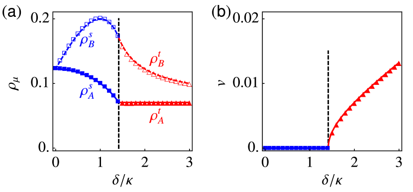
Figure 2: (a) Comparison of the amplitude of the first Fourier modes as obtained from simulations (symbols) and the one-mode approximations (lines): $\rho_{A}$ (solid line and filled symbols) and $\rho_{B}$ (dashed line and empty symbols) as functions of $\delta/\kappa$. (b) Velocity of the traveling pattern as a function of $\delta/\kappa$ from simulations (symbols) and one-mode approximation (line). In both (a) and (b) the black vertical dashed line denotes the critical value $\delta_{c}/\kappa=(1+\alpha_{B}^{2}/\kappa^{2})^{1/2}$ of the static-to-traveling transition. $\chi_{A}=-0.05$ is used in both panels.

Linear stability analysis.

A linear stability analysis of the fixed points yields the boundaries between the various states shown in Fig. 1a and provides a clear understanding of the mechanism of the drift instability. Linearizing  (3) about the homogeneous state reveals that in this state the dynamics of fluctuations is controlled by two eigenvalues given by

$$\lambda_{\pm}=-\frac{1}{2}(\alpha_{A}+\alpha_{B})\pm\frac{1}{2}\sqrt{(\alpha_{A}-\alpha_{B})^{2}+4(\kappa^{2}-\delta^{2})}\;.$$ (8)

If $\delta^{2}<\kappa^{2}+(\alpha_{A}-\alpha_{B})^{2}/4$, the eigenvalues are real. The largest eigenvalue $\lambda_{+}$ becomes positive, signaling an instability, when $\delta^{2}=\kappa^{2}-\alpha_{A}\alpha_{B}$. This diffusive instability is displayed as a blue line in Fig. 1a. It is a super-critical pitchfork bifurcation, where the trivial steady state $F_{H}$ undergoes spontaneous breaking of translational symmetry leading to the transition to the static phase-separated state $F_{S}$. Conversely, when $\delta^{2}>\kappa^{2}+(\alpha_{A}-\alpha_{B})^{2}/4$ the eigenvalues are complex conjugate. The state $F_{H}$ can still become unstable when $\alpha_{A}<-\alpha_{B}$, albeit now via an oscillatory instability shown as a red line in Fig. 1a.

Further insight is gained by examining the stability of $F_{S}$. This requires the analysis of the eigenvalues of the $3\times 3$ matrix obtained by linearizing (4a)-(4c). Details are given in the SI. Note that the matrix is block diagonal, coupling separately the two amplitudes and the phase difference $\theta$. One finds that the instability is driven by the growth of fluctuations in the relative phase $\theta$ that become unstable when $\delta>\delta_{c}$. This boundary $\delta=\delta_{c}$ corresponds to the appearance of $F_{T}$ and is shown as a black line in Fig. 1a. The instability of the relative phase is associated with the “run-and-catch” scenario described earlier and signals the transition to a state where the two fields have a constants phase lag (different from $\pi$), while traveling with a common speed.

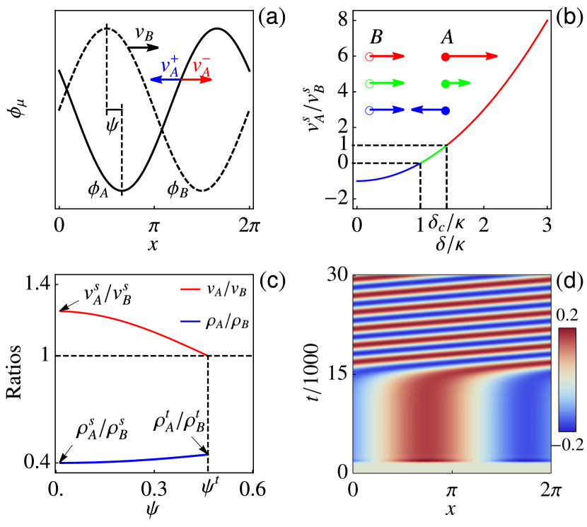
Figure 3: A pictorial explanation of the “run-and-catch” mechanism that leads to the stable traveling state. (a) A phase shift $\psi=\theta-\pi$ of $\phi_{A}$ (solid line) and $\phi_{B}$ (dashed line) relative to the out-of-phase modulation of the stationary demixed state results in finite velocities for the two fields. For a given $v_{B}$ (black arrow), $v_{A}$ is in the opposite (blue) or same (red) direction depending on whether the cross diffusivities have equal or opposite signs. (b) Ratio of velocities of the two species as given by (9) evaluated at the $F_{S}$ fixed point as a function of $\delta/\kappa$. The arrows are a depiction of the velocities obtained for a small finite $\psi$. Arrow colors correspond to the colors of each portion of the curve. (c) Ratio of the velocities (red) and amplitudes (blue) of the two species as functions of $\psi=\theta-\pi$ obtained from a simulation where the static pattern experiences a drift bifurcation and becomes traveling (i.e. panel d). The values at $\psi=0$ and $\psi=\psi^{t}=\theta^{t}-\pi$ agree with those obtained from the one-mode model. The horizontal dashed line corresponds to $v_{A}/v_{B}=1$ and the vertical dashed line is the value $\psi^{t}$ corresponding to the steady traveling state.(d) Spatiotemporal patterns at the onset of the static-to-traveling transition with $\delta/\kappa=1.5$. $\chi_{A}=-0.05$ is used.

To highlight the mechanism responsible for the traveling pattern, note that the velocity of the field modulations $v_{\mu}=\dot{\theta}_{\mu}$ are given by $v_{A}=\kappa_{AB}(\rho_{B}/\rho_{A})\sin\theta$ and $v_{B}=-\kappa_{BA}(\rho_{A}/\rho_{B})\sin\theta$, hence are identically zero in the static state $F_{S}$ where $\theta^{s}=\pi$. Now consider the effect of a small fluctuation in the relative phase by letting $\theta=\pi+\psi$, as shown in Fig. 3a. Evaluating the amplitudes at the steady state values, the velocities are then given by $v_{A}^{s}=-\frac{\kappa_{AB}\kappa_{BA}}{\alpha_{B}}\psi$ and $v_{B}^{s}=\alpha_{B}\psi$ (see Fig. 3b). If the cross-diffusivities $\kappa_{AB}$ and $\kappa_{BA}$ have the same sign, the two species move in opposite directions (black and blue arrows in Fig. 3a), exerting reciprocal driving forces on each other, and the perturbation $\psi$ decays. On the other hand, if $\kappa_{AB}$ and $\kappa_{BA}$ have opposite signs, the two species travel in the same direction (black and red arrows in Fig. 3a) and can play run-and-catch with each other. To establish the precise condition for the onset of the traveling state, it is useful to examine the ratio of the two velocity, which is well defined even in the static demixed state and is given by

$$\frac{v_{A}}{v_{B}}=-\frac{\kappa_{AB}\rho_{B}^{2}}{\kappa_{BA}\rho_{A}^{2}}=-\frac{(\kappa-\delta)\rho_{B}^{2}}{(\kappa+\delta)\rho_{A}^{2}}\;.$$ (9)

In the stationary demixed state, where $\rho_{B}^{s}/\rho_{A}^{s}=(\kappa+\delta)/\alpha_{B}$, we find $v_{A}^{s}/v_{B}^{s}=(\delta^{2}-\kappa^{2})/\alpha_{B}^{2}$. This quantity is shown in Fig. 3b. When $v_{A}^{s}/v_{B}^{s}<0$ (blue portion of the curve) a small fluctuation $\psi=\theta-\pi$ of the relative phase yields opposite field velocities (blue arrows), while when $v_{A}^{s}/v_{B}^{s}>0$ the velocities are in the same direction (green portion of the curve and green arrows). Only when $v_{A}^{s}/v_{B}^{s}>1$, however, nonreciprocity is strong enough to destabilize the static pattern (red line and arrows in Fig. 3b). The onset of the traveling state corresponds to $v_{A}^{s}=v_{B}^{s}$ or $\delta=\delta_{c}$, as obtained from the linear stability analysis. The condition $v_{A}=v_{B}$ provides a general necessary condition for the onset of traveling patterns of two interacting scalar fields.

The equality of the velocities is not, however, sufficient to stabilize the traveling pattern as the perturbation $\psi$ will keep increasing if $v_{A}>v_{B}$ persists. Non-reciprocal interactions come again to the rescue by facilitating the “redistribution” of amplitude growth. Specifically, as $\psi$ increases, both the damping of $\rho_{A}$ and the activation of $\rho_{B}$ originating from the non-reciprocal nature of the cross couplings become weaker (last terms in (4a)-(4b)). Consequently, the amplitude ratio $\rho_{A}/\rho_{B}$ increases and suppresses the velocity difference until $v_{A}=v_{B}$, allowing the development of a steady traveling pattern, as shown in Fig. 3c. We have validated this simple picture displayed in Fig. 3d by examining numerically the mechanisms of stabilization of the traveling state $F_{T}$ for $\delta$ slightly larger than $\delta_{c}$.

III Static-to-traveling as a PT-breaking transition

The static-to-traveling transition described in this work belongs to a more generic class of PT-breaking transitions Coullet et al. (1989); El-Ganainy et al. (2018); Hanai and Littlewood (2019), which has been studied in optical and quantum systems Lin et al. (2011); Hanai and Littlewood (2019) and more recently in polar active fluids with non-reciprocal interactions Fruchart et al. (2020). This type of transition is known to occur at a so-called exceptional point, which is simply a point where the eigenvalues of the matrix that governs the linear stability of a fixed point become equal and its eigenvectors are co-linear. While not uncommon in hydrodynamics when fluids are driven by external forces or in systems described by non-conserved fields, the occurrence of such a transitions giving rise to nontrivial traveling structures in conserved systems is unexpected.

The dynamics of our coupled fields can be written in a compact form as

$$\partial_{t}\begin{pmatrix}\phi_{A}\\ \phi_{B}\end{pmatrix}=\mathbf{M}\cdot\begin{pmatrix}\phi_{A}\\ \phi_{B}\end{pmatrix}\;,$$ (10)

where the $2\times 2$ matrix operator $\mathbf{M}=\mathbf{M}[\phi_{A}^{2},\phi_{B}^{2},\nabla^{2}]$ can be inferred from (1). In the static, spatially modulated solution corresponding to the demixed state, the two fields $\phi_{A}$ and $\phi_{B}$ are out of phase, but have the same parity under spatial inversion, $x\rightarrow-x$, as required by the symmetry of $\mathbf{M}$. The domains become traveling by acquiring a component of the opposite parity that breaks the relative parity of the two fields, as described in Ref. Coullet et al. (1989). Hence the transition to the traveling state breaks both parity and time reversal invariance.

This is most easily understood in the context of the one-mode approximation by considering a static $F_{S}$ solution of the form $\phi_{B}=\rho_{B}\cos(x)$ and $\phi_{A}=\rho_{A}\cos(x+\pi)$. Both fields are even and are out of phase, but have different amplitudes. A perturbation $\psi$ in the phase difference yields $\phi_{A}=\rho_{A}\cos(x+\pi+\psi)=\rho_{A}\left[-\cos\psi\cos x+\sin\psi\sin x\right]$, breaking parity as $\phi_{A}$ now acquires an odd component. The response to such a perturbation is governed by (4c) linearized about the steady state for $\delta\rightarrow\delta_{c}$, which is given by

$$\dot{\psi}\simeq\frac{2\delta_{c}(\delta-\delta_{c})}{\alpha_{B}}\psi\;.$$ (11)

For $\delta<\delta_{c}$, the odd component of $\phi_{A}$ proportional to $\psi$ decays, restoring the parity of the static solution. For $\delta>\delta_{c}$, $\psi$ grows to a finite value, destabilizing the static state. As a result, $\phi_{A}$ acquires a finite odd component, breaking the parity of the static solution. Meanwhile, near the transition (4d) gives $\dot{\Phi}_{T}\simeq 2\alpha_{B}\psi$, resulting in a finite $\dot{\Phi}$ for $\delta>\delta_{c}$ and breaking time reversal symmetry.

IV Discussion and outlook

We have shown that non-reciprocal effective interactions in a minimal model of conserved coupled fields with purely diffusive dynamics lead to a PT-breaking transition to traveling spatially modulated states. While the emergence of traveling spatio-temporal patterns is well known in reaction-diffusion, prey-predators and related models, its appearance in the dynamics of conserved fields without external forcing is surprising. Although the work presented here is limited to a minimal model in one dimension, preliminary results shown in the SI indicate that the same mechanism is at play in two dimensions, as well as in mixtures of active and passive particles and of particles interacting via competing repulsive and attractive interactions, as may be realized in phoretic colloidal mixtures. We speculate therefore that the mechanism described here through which non-reciprocal effective couplings grant motility to static spatial modulations may be a generic property of multispecies systems describes by scalar fields.

The type of static-to-traveling transition described here occurs in Mullins-Sekerka models of crystal growth Mullins and Sekerka (1964), Keller-Segel, prey-predator and reaction-diffusion models of population dynamics and general systems described by non-conserved dynamical fields, where it has been referred to as a drift bifurcation Coullet et al. (1989); Fauve et al. (1991); Biktashev and Tsyganov (2009). It occurs in these systems when a stationary or standing wave pattern generated through a conventional Hopf bifurcation undergoes a second instability to a traveling state. The drift bifurcation can be understood using amplitude equations as arising from the antagonistic coupling of at least two leading modes Fauve et al. (1991). Here we show that a similar mechanism can be at play in multispecies systems with dynamics described by two conserved scalar fields coupled by sufficiently strong nonreciprocal interactions. When sufficiently strong, nonreciprocity leads to an effective antagonistic repulsion/attraction between the two fields, resulting in the run-and-catch mechanism described here that yields a PT-symmetry breaking transition. Our one-mode approximation provides a minimal analytic description of this generic mechanism, where $v=\dot{\Phi}/2$ serves as the order parameter for the transition.

A scenario similar to the one described here was recently identified in a binary Vicsek model with non-reciprocal interactions Fruchart et al. (2020). The mechanisms promoting the onset of a state with broken PT are the same in both models, but the outcomes are distinct due to the different symmetry of the two systems. In Ref. Fruchart et al. (2020) it is suggested that non-reciprocal interaction in a polar system may generically result in macroscopically chiral phases. Here, in contrast, we consider a scalar model with conserved dynamics and demonstrate that in this case non-reciprocity generically yields spatially inhomogeneous traveling states through the same type of PT-breaking transition. Together, these works pave the way to the study of the interplay of non-reciprocity and spontaneously-broken symmetry, suggesting a path to the classification of a new type of PT-breaking transitions.

Understanding and quantifying the role of non-reciprocity in controlling nonequilibrium pattern formation has direct implication to the assembly of chemically interacting colloids, where different particles naturally produce different chemicals mediating nonreciprocal couplings that can induce the type of chasing behavior seen in our work. It also provides a general framework for understanding the nature of wave and oscillatory behavior seen ubiquitously in systems with non-conserved field, from diffusion reaction to prey-predator and population dynamics models. Our predictions can be tested in detailed simulations of active-passive colloidal mixtures or of particles with antagonistic interactions, as well as experiments in mixtures of chemically driven microswimmers.

Our work opens up many new directions of inquiry. Obvious extensions are to higher dimensions where we expect a richer phase diagram and to systems with birth and death processes that select a scale of spatial patterns Cates et al. (2010). The exploration of the role of nonreciprocal interactions in active matter systems with broken orientational symmetry, either polar or nematic, is only beginning Fruchart et al. (2020) and promises to reveal a rich phenomenology. Chemically mediated or other nonequilibrium couplings can often be time-delayed, which can provide an additional, possibly competing mechanism for the emergence of oscillatory behavior. Finally, an important open problem is understanding how nonreciprocity arises as an emergent property in systems with microscopic reciprocal interactions, such as active-passive mixtures.