Edit Distance in Near-Linear Time: it’s a Constant Factor

Abstract

We present an algorithm for approximating the edit distance between two strings of length $n$ in time $n^{1+\epsilon}$ up to a constant factor, for any $\epsilon>0$. Our result completes a research direction set forth in the recent breakthrough paper [CDG⁺18], which showed the first constant-factor approximation algorithm with a (strongly) sub-quadratic running time. The recent results [KS20b, BR20] have shown near-linear time algorithms that obtain an additive approximation, near-linear in $n$ (equivalently, constant-factor approximation when the edit distance value is close to $n$). In contrast, our algorithm obtains a constant-factor approximation in near-linear time for any input strings.

In contrast to prior algorithms, which are mostly recursing over smaller substrings, our algorithm gradually smoothes out the local contribution to the edit distance over progressively larger substrings. To accomplish this, we iteratively construct a distance oracle data structure for the metric of edit distance on all substrings of input strings, of length $n^{i\epsilon}$ for $i=0,1,\ldots,1/\epsilon$. The distance oracle approximates the edit distance over these substrings in a certain average sense, just enough to estimate the overall edit distance.

1 Introduction

Edit distance is a classic distance measure between sequences that takes into account the (mis)alignment of strings. Formally, edit distance between two strings of length $n$ over some alphabet $\Sigma$ is the number of insertions/deletions/substitutions of characters to transform one string into the other. Being of key importance in several fields, such as computational biology and signal processing, computational problems involving the edit distance were studied extensively.

Computing edit distance is also a classic dynamic programming problem, with a quadratic run-time solution. It has proven to be a poster challenge in a central theme in TCS: improving the run-time from polynomial towards close(r) to linear. Despite significant research attempts over many decades, little progress was obtained, with a $O(n^{2}/\log^{2}n)$ run-time algorithm [MP80] remaining the fastest one known to date. See also the surveys of [Nav01] and [Sah08]. With the emergence of the fine-grained complexity field, researchers crystallized the reason why beating quadratic-time is hard by connecting it to the Strong Exponential Time Hypothesis (SETH) [BI15] (and even more plausible conjectures [AHWW16]).

Even before the above hardness results, researchers started considering faster algorithms that approximate edit distance. A linear-time $\sqrt{n}$-factor approximation follows immediately from the exact algorithm of [Ukk85, Mye86, LMS98], which runs in time $O(n+d^{2})$, where $d$ is the edit distance between the input strings. Subsequent research improved the approximation factor, first to $n^{3/7}$ [BJKK04], then to $n^{1/3+o(1)}$ [BES06], and to $2^{\tilde{O}(\sqrt{\log n})}$ [AO12] (based on the $\ell_{1}$ embedding of [OR07]). In the regime of $O(n^{1+\epsilon})$-time algorithms, the best approximation is $(\log n)^{O(1/\epsilon)}$ [AKO10]. Predating some of this work was the sublinear-time algorithm of [BEK⁺03] achieving $n^{\epsilon}$ approximation when $d$ is large.

In a recent breakthrough, [CDG⁺18] showed that one can obtain constant-factor approximation in $O(n^{12/7})$ time. Subsequent developments [KS20b, BR20] give $O(n^{1+\epsilon})$-time algorithms for computing edit distance up to an additive $n^{1-g(\epsilon)}$ term and $f(1/\epsilon)$-factor approximation, for some non-decreasing functions $f,g$, and any $\epsilon>0$.

Our main result

is a $n^{1+\epsilon}$ algorithm for computing the edit distance up to a constant approximation.

Theorem 1.1.

For any $\epsilon>0$, $n\geq 1$, and alphabet $\Sigma$, there is a randomized algorithm that, given two strings $x,y\in\Sigma^{n}$, approximates the edit distance between $x$ and $y$ in $O(n^{1+\epsilon})$ time up to $f(1/\epsilon)$-factor approximation, where $f(1/\epsilon)$ depends solely on $\epsilon$.

While we do not derive the function $f(1/\epsilon)$ explicitly, we note that it is doubly exponential in $1/\epsilon$. We present a technical overview of our approach in Section 3, after setting up our notations in Section 2. The proof of the main theorem will follow in subsequent sections, in particular the top-level algorithm and its main guarantees are in Section 4.

1.1 Related work

A quantum algorithm for edit distance was introduced in [BEG⁺18]. Some of the basic elements of the algorithmic approach are related to [CDG⁺18] (and the algorithm in this paper). Another recent related paper is [GRS20], who obtain $3+\epsilon$ approximation in $\tilde{O}(n^{1.6})$ time; independently, the first author obtained a slightly worst time for the same approximation [And18]. Similarly, independently, [CDK19] and [And18] extended the constant-factor edit distance algorithm from [CDG⁺18] to solve the text searching problem.

Sublinear time algorithms have drawn renewed attention [GKS19, KS20a, BCR20, BCFN22, GKKS22]; see also earlier [BEK⁺03, BJKK04, AO12]. Another related line of work has been on computing edit distance for the semi-random models of input [AK12, Kus19]. Parallel (MPC) algorithms were developed in [BEG⁺18, HSS19].

Progress on edit distance algorithms also inspired the first non-trivial algorithms for approximating the longest common subsequence (LCS) [HSSS19, RSSS19, RS20, BCAD21], leading to a linear time, $n^{o(1)}$-approximation algorithm [ANSS22, Nos21]. Also of note is [RS20] which shows that a $O(1)$-factor approximation to edit distance implies a $2-\Omega(1)$ factor approximation to LCS over a binary alphabet in (essentially) the same time.

1.2 Acknowledgements

We would like to thank FOCS and SICOMP anonymous reviewers for helpful comments and suggestions that helped improve this paper.

2 Preliminaries: Setup and Notations

Fix a pair of strings $(x,y)\in\Sigma^{n}\times\Sigma^{n}$ for which we care to estimate the edit distance. We define $\mathtt{ed}_{n}(x,y)$ as half the number of insertions/deletions to transform one string into the other. Note that the standard edit distance (allowing substitutions) can be reduced to this case (see, e.g., [Tis08]). When length $n$ is clear from the context, we omit the subscript.

$S_{w}$ is the set of integer powers of 2 up to $w$: namely, $S_{w}=\{1,2,4,8\ldots w\}\cup\{1/2,1/4\ldots 1/2n\}$.

$[n]$ denotes the set $\{1,2,3,\ldots n\}$ throughout the paper except where stated explicitly otherwise (notably, in Section 9).

When describing intuitive parts, we sometimes use $O^{*}(f(n))$ to denote $f(n)\cdot n^{O(\epsilon)}$ (where $\epsilon$ is the small constant from the algorithm).

Finally, we use the standard notion of with high probability (whp), meaning with probability at least $1-n^{-C}$ for large enough constant $C>1$.

2.1 Intervals

An interval is a substring $x[i:j]\triangleq x_{i}x_{i+1}\ldots x_{j-1}$, for $i,j\in[n]$, where $i\leq j$ (i.e., starting at $i$ and ending at $j-1$, of length $j-i$).

For $i\in[n]$, let $X_{i,w}$ ($Y_{i,w}$) denote the interval of $x$ ($y$) of length $w$ starting at position $i$. Let $\mathcal{X}_{w},\mathcal{Y}_{w}$ the set of all such $X_{i,w}$ and $Y_{j,w}$ strings respectively. We use $\mathcal{I}_{w}=\mathcal{X}_{w}\cup\mathcal{Y}_{w}$ to denote all $x$ and $y$ axis intervals. When clear from context, we drop subscript $w$.

By convention, if $i\not\in[1,n-w]$, we pad $X_{i}/Y_{i}$ with a default character, say, $. Also $Y_{\bot,w}$ is a string of unique characters. In particular, for all distance functions $\tau_{w}(\cdot,\cdot)$ on two length-$w$ strings in this paper, we define $\tau_{w}(X_{i,w},Y_{\bot,w})=w$; e.g., $\mathtt{ed}_{w}(X_{i,w},Y_{\bot,w})=w$.

Usually, by $I\in\mathcal{I}_{w}$ we refer not only to the corresponding substring but also to the “meta-information”, in particular the string it came from, start position, and length (e.g., for $I=X_{i,w}$, the meta-information is $x,i,w$). This difference will be clear from context or stated explicitly.

In particular, the notation $I+j$, for an interval $I$ and integer $j$, represents the interval $j$ positions to the right; e.g., if $I=X_{i,w}$, then $I+j=X_{i+j,w}$.

Alignments.

An alignment between $x$ and $y$ is a function $\pi:[n]\to[n]\cup\{\bot\}$, which is injective and strictly monotone on $\pi^{-1}([n])$. The set of all such alignments is called $\Pi$. Note that $\mathtt{ed}(x,y)=\min_{\pi\in\Pi}\sum_{i\in[n]}\mathtt{ed}_{1}(x_{i},y_{\pi(i)})$ (recall that, by convention, $\mathtt{ed}_{1}(c,y_{\bot})=1$ for all $c\in\Sigma$).

It is convenient for us to think of $\pi$ as function from $\mathcal{I}\rightarrow\mathcal{I}$, via the following extension. For a given input alignment $\pi:{\mathcal{X}}\rightarrow{\mathcal{Y}}\cup\{\bot\}$, its extension $\widehat{\pi}:\mathcal{I}\rightarrow\mathcal{I}\cup\{\bot\}$ is:

$$\widehat{\pi}[I]=\begin{cases}\pi[I]&I\in{\mathcal{X}}\\ \pi^{-1}[I]&I\in{\mathcal{Y}}\end{cases},$$

where $\widehat{\pi}[X_{i,w}]$ means $Y_{\pi(i),w}$, and $\widehat{\pi}[Y_{j,w}]$ means $X_{\pi^{-1}(j),w}$, with $\pi^{-1}(j)=\bot$ if there’s no $i$ with $\pi(i)=j$. Throughout this paper, we overload notation to use $\pi$ for the extension $\widehat{\pi}$ as well. We also define ${\overleftarrow{\pi}}(i)$ as the minimum $\pi(j)$, $j\geq i$, which is defined ($\neq\bot$).

Finally, we also define $\pi(i)\triangleq i$ when $i<1$ and $i>n$ for convenience.

2.2 Interval distances

Our algorithms will use distances/metrics over intervals in $\mathcal{I}_{w}$. One important instance is the alignment distance, denoted $\mathtt{ad}_{w}(\cdot,\cdot)$. At a high level, $\mathtt{ad}_{w}(\cdot,\cdot)$ is a distance metric that approximates edit distance on length-$w$ intervals. We discuss $\mathtt{ad}(\cdot,\cdot)$ metric in Section 4 as well as 9.

Definition 2.1 (Neighborhood).

Fix $c\geq 0$ and $I\in\mathcal{I}_{w}$. The $c$-neighborhood of $I$ is the set $\mathcal{N}_{c}(I)=\{J\in\mathcal{I}_{w}\mid\mathtt{ad}(I,J)\leq c\}$, i.e. all $x$ and $y$ intervals which are $c$-close to $I$ in terms of their alignment distance.

Definition 2.2 (Ball of intervals).

A ball of intervals is a set of consecutive intervals in either ${\mathcal{X}}_{w}$ or ${\mathcal{Y}}_{w}$ (i.e., it’s a ball in the metric where distance between $X_{i}$ and $X_{j}$ is $|i-j|$). The smallest enclosing ball of a set ${\mathcal{S}}$ is the minimal ball $\mathcal{B}\supseteq{\mathcal{S}}$.

Average approximation for an optimal alignment.

A common theme in our algorithm is constructing metrics on $\mathcal{I}_{w}$ approximating $\mathtt{ed}_{w}$ in a certain “average sense”. In particular, this differs from the standard notion of approximation in that the upper bound holds only on average, and for an optimal alignment $\pi\in\Pi$. Formally, we define:

Definition 2.3 (Align-approximation).

Fix space $(\mathcal{I}_{w},{\mathsf{d}})$ over $\mathcal{I}_{w}$ (which is often a metric space, but need not be). We say ${\mathsf{d}}$ $T$-align-approximates $\mathtt{ed}$ if the following holds:

1. For all $I,J\in\mathcal{I}_{w}$: ${\mathsf{d}}(I,J)\geq\mathtt{ed}_{w}(I,J)$.

2. $\min_{\pi\in\Pi}\sum_{i\in[n]}\tfrac{1}{w}{\mathsf{d}}(X_{i},Y_{\pi(i)})\leq T\cdot\mathtt{ed}(x,y).$

2.3 Operations on sets and the $*$ notation

By convention, applying numerical functions to a set refers to the sum over all set items; e.g., $f(S)=\sum_{i\in S}f(i)$. When applying set operators on other sets, we use the union; e.g., $\pi({\mathcal{S}})=\cup_{I\in{\mathcal{S}}}\pi(I)$ and $\mathcal{N}_{c}({\mathcal{S}})=\cup_{I\in{\mathcal{S}}}\mathcal{N}_{c}(I)$. Abusing notation, we use $f(S)$ even when $S$ is not fully contained in the domain of $f$ — in which case, we simply ignore elements outside the domain. Any exception to the above will be clearly specified.

We also use the notation $*$ as argument of a function, by which we mean a vector of all possible entries. E.g., $f(*)$ is a vector of $f(i)$ for $i$ ranging over the domain of $f$ (usually clear from the context). Similarly, $f(*_{\mathcal{R}})$ means a vector of $f(i)$ for $i$ satisfying property ${\mathcal{R}}$. Overloading notation, sometimes $f(*_{\mathcal{R}})$ will also mean a vector of $f(i)$ for all $i$ in the domain, with coordinates $i\notin{\mathcal{R}}$ being zeroed-out.

3 Technical Overview

3.1 Prior work and main obstacles

As our natural starting point is the breakthrough $O(n^{12/7})$-time algorithm of [CDG⁺18] (and related [BEG⁺18]), we first describe their core ideas as well as the challenges to obtaining a near-linear time algorithm. In particular, we highlight two of their enabling ideas. At a basic level, their algorithm computes edit distance $\mathtt{ed}_{n}(x,y)$ by computing $\mathtt{ed}_{w}$ between various length-$w$ intervals (substrings) of $x,y$ recursively, and then uses edit-distance-like dynamic programming on intervals to put them back together. The main algorithmic thrust is to reduce the number of recursive $\mathtt{ed}_{w}$ computations: e.g., if the intervals are of length $w$, and we only consider non-overlapping intervals, there are still $n/w\times n/w$ calls to $\mathtt{ed}_{w}$, each taking at best $\Omega(w)$ time. Hence, [CDG⁺18] employ two ideas to do this efficiently: 1) use the triangle inequality to deduce distance between pairs of intervals for which we do not directly estimate $\mathtt{ed}_{w}$, 2) two nearby $x$-intervals (e.g., consecutive) are likely to be matched into two nearby $y$-intervals (also consecutive) under the optimal edit distance alignment $\pi$. (The earlier quantum result [BEG⁺18] employed the first idea already, but relied on a quantum component instead of the second idea.) Indeed, these ideas are enough to reduce the number of recursive calls from $(n/w)^{2}$ to $\approx(n/w)^{1.5}$.

One big challenge in the above is that, in general, one has to consider all, overlapping intervals from $x,y$, of which there are $n$ — since, in an optimal $\mathtt{ed}_{n}$ alignment, an $x$-interval might have to match to a $y$-interval whose start position is far from an integer multiple of $w$. An alternative perspective is that if one considers only a restricted set of interval start positions, say every $s\leq w$ positions in $y$, then one obtains an extra additive error of about $s\cdot n/w$ from the “rounding” of start positions in $y$. That’s the reason that a bound of $(n/w)^{1.5}$ recursive calls did not transform into $n^{1.5}$ runtime in [CDG⁺18]: to compute edit distance when $\mathtt{ed}<n^{1-\Omega(1)}$, they employ a standard (exact) $\tilde{O}(n+\mathtt{ed}^{2}(x,y))$ algorithm [Ukk85, Mye86].

Recent improvements by [KS20b, BR20] showed how to reduce the number of recursive calls to $\approx n/w$, but some fundamental obstacles remained. The linear number of recursive calls was leveraged to obtain near-linear time but with an additive approximation only: when $\mathtt{ed}(x,y)\geq n^{1-\delta}$, the overall runtime is $n^{1+f(\delta)}$ for some increasing function $f$.

In particular, in addition to the aforementioned challenge, a new challenge arose: to be able to reduce to near-linear number of recursive $\mathtt{ed}_{w}$ calls, the algorithms from [KS20b, BR20] might miss a large fraction of “correct” matches. In particular this fraction is $\approx n^{-\delta}$, which results in an additive error of $\approx n^{1-\delta}$. To put this into perspective, for $w=\sqrt{n}$, if we allow an additive error $n^{1-\delta}$, then it suffices to analyze $b=n^{0.5+O(\delta)}$ intervals (which barely overlap) and misclassify $b\cdot n^{-\delta}$ of them. We use the following example to showcase the challenges:

A running example illustrating the challenges Consider an instance where $\Delta=n^{-0.01}$ fraction of intervals in ${\mathcal{X}}_{w}$ are “sparse” — have a single cheap match in ${\mathcal{Y}}_{w}$ — and the rest of the intervals are dense (they are close to many other intervals). Assume further that such sparse intervals are spread around in multiple “sparse sections” (sequences of consecutive sparse intervals).

Note that if we can afford large additive errors, we can simply ignore all these sparse intervals (certifying them at max cost $w$) and output the distance based on the dense intervals only, with at most $n\Delta=n^{0.99}$ additive approximation. To avoid this, one must first identify some sparse intervals (since the dense intervals do not provide sufficient information about the sparse sections). Even if we manage to find some of the sparse intervals efficiently, we still need to apply knowledge of the location of such intervals to deduce information on other intervals which might be in completely different areas in the string. We will return to this example later.

Below we describe the high-level approach to our algorithm, including how we overcome these obstacles. We note that, while our algorithm is based on the two key ideas from [CDG⁺18], the high-level algorithm departs from the general approach undertaken in [CDG⁺18, KS20b, BR20]. That said, some algorithmic steps are similar to those developed in [KS20b, BR20]. We do not rely on previous results (for any distance regime) such as [Ukk85].

3.2 Our high-level approach

While there are many ideas going in overcoming the above challenges, one common theme is averaging over the local proximity of intervals. In particular, the algorithm proceeds by, and analyzes over, “average characteristics” of various intervals of $x,y$, in a “smooth” way. For example decisions for a fixed interval $I\in\mathcal{I}_{w}$, such as whether something is close, or something is matched, are done by considering the statistics collected on nearby intervals (to the left/right of $I$ in the corresponding string). While we expand on our technical ideas below, this is the guiding principle to keep in mind.

Addressing the first challenge, we consider intervals (of fixed length $w$) at all $n$ starting positions, i.e., the entire set $\mathcal{I}_{w}$. Note that recursion becomes prohibitive: we can’t perform even $n$ edit distance evaluations each taking $\Omega(w)$ time ($w$ is set to be $\approx n^{1-\epsilon}$). Instead, our top-level algorithm iterates bottom–up over all interval lengths $w=\gamma,\gamma^{2},\ldots n$, where $\gamma=n^{\epsilon}$, and for each $w$ computes a good-enough approximation to the entire metric $(\mathcal{I}_{w},\mathtt{ed}_{w})$. Recall that $\mathcal{I}_{w}=\mathcal{X}_{w}\cup\mathcal{Y}_{w}$ consists of all $w$-length intervals (substrings); i.e., $|\mathcal{I}_{w}|=2n$. The metric, termed $\mathfrak{D}_{w}(\cdot,\cdot)$, will be accessible via a distance oracle (fast data structure), with $n^{\epsilon}$ query time, and will approximate the distance between most of the pairs (an $x$-interval, $y$-interval) that participate in an optimal alignment in an average sense. Specifically, for $\pi$ ranging over all alignments, we will have that $\min_{\pi}\tfrac{1}{w}\mathfrak{D}_{w}(X_{i,w},Y_{\pi[i],w})=\Theta(\mathtt{ed}(x,y))$. Formally, we say $\mathfrak{D}_{w}$ $O(1)$-align-approximates $\mathtt{ed}$ (see Def. 2.3).

In each iteration, we build $\mathfrak{D}_{w}$ using $\mathfrak{D}_{w^{\prime}}$, where $w^{\prime}=w/\gamma$. Conceptually we do so in two phases. First, we build another metric on $w$-length strings, $(\mathcal{I}_{w},\mathtt{ad}_{w})$, accessible via a fast distance oracle, that uses $\gamma^{O(1)}=n^{O(\epsilon)}$ time and $\mathfrak{D}_{w^{\prime}}$ oracle calls. Crucially, $\mathtt{ad}_{w}$ will similarly align-approximate $\mathtt{ed}$. Second, equipped with a fast oracle for $\mathtt{ad}_{w}$ (itself using $\mathfrak{D}_{w^{\prime}}$), we build an “efficient representation” for the entire metric $(\mathcal{I}_{w},\mathtt{ad}_{w})$, while using only $n^{1+O(\epsilon)}$ calls to $\mathtt{ad}_{w}$ oracle. Naturally, this “efficient representation” will not be able to capture the entire $\mathtt{ad}_{w}$ metric (that would require $\gg n$ query complexity), but it will capture just enough to preserve the edit distance between $x$ and $y$—again, formally, align-approximate $\mathtt{ed}$. Then we build an efficient distance oracle for this efficient representation, which will yield the desired metric $\mathfrak{D}_{w}$. Note that the final approximation to $\mathtt{ed}(x,y)$ is computed by (essentially) querying $\mathfrak{D}_{n}(X_{1,n},Y_{1,n})$.

In particular, the “efficient representation” of $\mathtt{ad}_{w}$ is a weighted graph $G_{w}$ with vertex set $\mathcal{I}_{w}$ and $n^{1+\epsilon}$ edges, such that the shortest path between $I,J\in\mathcal{I}_{w}$ approximates $\mathtt{ad}_{w}(I,J)$, again, in an average sense for an optimal alignment. In particular, the shortest path distance is non-contracting, and non-expanding for interval pairs that “matter”, i.e., which are part of the optimal alignment $\pi$ corresponding to $\mathtt{ed}(x,y)$. An edge $(I,J)$ of the graph $G_{w}$ will always correspond to an explicit call to $\mathtt{ad}_{w}(I,J)$; and the main question in constructing $G_{w}$ is deciding which $n^{1+\epsilon}$ pairs to compute $\mathtt{ad}_{w}$ for.

Once we have the graph $G_{w}$, we build a fast distance oracle data structure on it to obtain the metric $\mathfrak{D}_{w}$. In particular, our fast distance oracle is merely an embedding of the shortest path metric on $G_{w}$ into $\ell_{\infty}^{d}$, where $d=|\mathcal{I}|^{\epsilon}$, incurring an approximation of $O(1/\epsilon)$, via [Mat96]. We note that we cannot use some other common distance oracle, such as, e.g., [TZ05, Che14], because they do not guarantee that the resulting output is actually a metric, and in particular, that it satisfies the triangle inequality, which is crucial for us (as mentioned above). We remark that this particular step is somewhat reminiscent of the approach from [AO12], who similarly build an efficient representation for the metric $(\mathcal{I}_{w},\mathtt{ed}_{w})$ using metric embeddings. However, the similarity ends here: first [AO12] used Bourgain’s embedding into $\ell_{1}$, which incurs $\Theta(\log n)$ distortion, and second, more importantly, the construction of $G_{w}$ was altogether different (incurring a much higher approximation).

Computing the graph $G_{w}$ itself is the most algorithmically novel part of our approach, and is termed Interval Matching Algorithm, as it corresponds to matching intervals that are close in $\mathtt{ad}_{w}$ distance. This algorithmic part should be thought of as the analogue of the algorithm deciding for which pairs of intervals to (recursively) estimate the edit distance in [CDG⁺18].

We sketch the Interval Matching Algorithm next in this technical overview. We also sketch how to compute the $\mathtt{ad}_{w}$ distance in $n^{O(\epsilon)}$ time, which presents its own new challenges, especially to guarantee its metric properties.

3.3 Interval matching algorithm

The main task here is to efficiently compute a graph $G_{w}$ that approximates $\mathtt{ad}_{w}$, in an average sense over an optimal alignment $\pi$. Specifically, to generate $G_{w}$, we iterate over all costs $c\in S_{w}$ (powers of 2), and for each such cost, we then generate a (sub-)graph $G_{w,c}$, with edges of weight $\Theta(c)$. The following is the main guarantee: for any fixed alignment $\pi$, for any pair $(I,\pi[I])\in\mathcal{I}_{w}^{2}$ at a distance $\mathtt{ad}(I,\pi[I])\leq c$, we generate a 1- or 2-hop path for it in $G_{w,c}$—except for $O(k_{c})$ such pairs $(I,\pi[I])$ where $k_{c}$ is the number of pairs with $\mathtt{ad}(I,\pi[I])>c$ (i.e., the “error” increases by at most a constant factor). The union of such graphs $G_{w,c}$ yields the final graph $G_{w}$. Below we focus on a single scale graph $G_{w,c}$, which is supposed to capture nearly all pairs $(I,\pi[I])$ where $\mathtt{ad}_{w}(I,\pi[I])\leq c$. We refer to such a pair as a $\pi$-matchable pair $(I,\pi[I])$.

At its core, our algorithm can be thought of as a partitioning algorithm, where we partition $\mathcal{I}_{w}$ into sets of intervals, such that for nearly all $\pi$-matchable pairs $(I,\pi[I])$, both intervals belong to the same set. We start with a single set of intervals and we iteratively partition the set into progressively more refined partitions (consisting of smaller parts), with the goal of keeping $\pi$-matchable pairs $I,\pi[I]$ together. (This algorithm will use a significant amount of notation, and, while this high-level overview will mention only a fraction of them, the reader may refer to the Table 2 in Sec. 6 for some important definitions and formulas.)

In particular, the matching algorithm proceeds in $\approx 1/\epsilon$ steps. In each step $t$, for $\lambda=n^{\epsilon}$, we generate $\lambda^{t}$ parts, each of size $\lesssim n/\lambda^{t}$. To construct a part, we sample a random interval $A$, termed anchor, and estimate $\mathtt{ad}_{w}(A,I)$ for all other intervals $I$ in its part, generating a cluster of intervals at distance $O(c)$ from the anchor. The main desideratum is that the two intervals from a $\pi$-matchable pair $I,\pi[I]$ are either both close to $A$ or both far from $A$, and hence always remain together (this is related to the triangle inequality idea from [CDG⁺18]). However, this cannot be guaranteed, and ensuring this desideratum is a major challenge for us, which we will address later. For now, in order to build intuition, we first develop our ideas under the following the assumption, that the desideratum holds:

Perfect Neighborhood Assumption (PNA):

any two intervals are at distance either $\leq c$ or $\omega(c)$; hence $\mathcal{N}_{O(c)}(I)=\mathcal{N}_{c}(I)$.

Every anchor will generate precisely one part, of target size. Notice that if the cluster is sufficiently large (i.e., $\gtrsim n/\lambda^{t}$), we are basically done, and in fact, is where our algorithm “converges” (as will be described later). Otherwise, we use the cluster to construct one part (set) by taking the clustered intervals together with their local extensions: intervals around the clustered intervals (to the left/right of the clustered ones). The parameters are set up such that the resulting part has size $\lesssim n/\lambda^{t}$. Note that the iterative nature of the process helps ensure the runtime: As the size of parts decreases with step $t$, we can afford to use more anchors. In particular, at step $t$, we start with $\lambda^{t-1}$ partitions, each of size about $n/\lambda^{t-1}$, and hence, for each of $\lambda^{t}$ anchors, we need to estimate $\mathtt{ad}$ distance to $n/\lambda^{t-1}$ intervals (in its part), for an overall of $n\lambda$ distance computations.

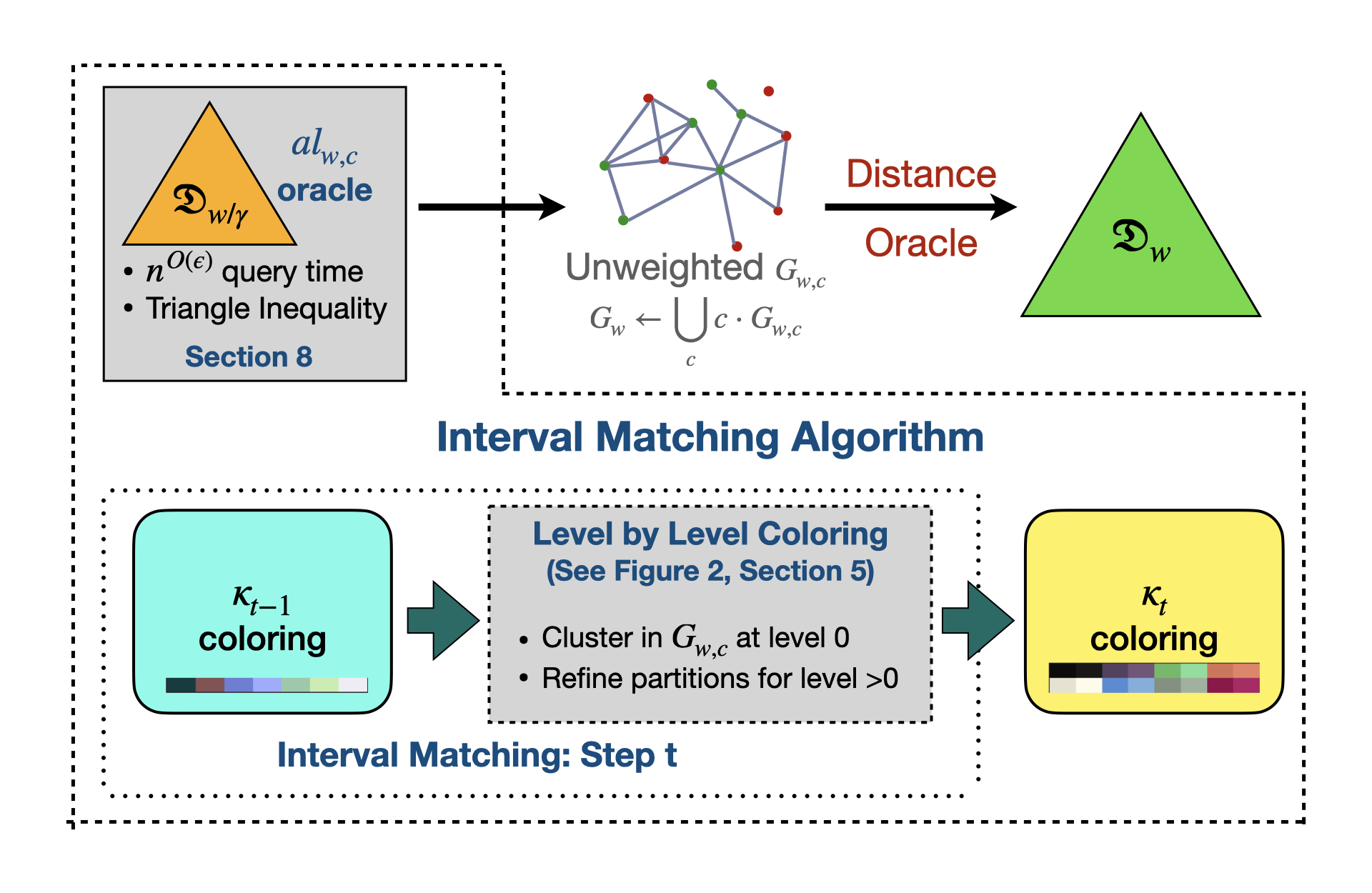
Figure 1: High Level Algorithm Scheme (Section 4)

A direct implementation of partitions as above however runs in various issues, yielding additive errors. In particular, it only guarantees to correctly partition “any fixed $\pi$-matchable pair with some probability”; instead of the needed “with some probability, all except a few $\pi$-matchable pairs are partitioned correctly” (akin to the “for each” vs “for all” guarantees). For the latter goal, bounding the “except a few” so that it’s only a $O(1)$-factor approximation, we use the notion of corruption, defined later.

Colorings.

To describe a partition, we use the slightly generalized concept of a coloring: a coloring $\kappa$ is a mapping from each interval $I\in\mathcal{I}$ to a distribution of colors in a color-set $\nu$, where a fixed color should be thought of as a part. We denote the mapping by $\mu_{\kappa}:\mathcal{I}\times\nu\rightarrow[0,1]$. For each interval $I$, we require $\|\mu_{\kappa}(I,*)\|_{1}=1$, i.e., we think of the interval $I$ as being split into fractions each assigned to a part: fraction $\mu_{\kappa}(I,\chi)>0$ is assigned to color $\chi$. While under the “perfect neighborhood assumption”, standard partitions are sufficient (i.e., $\mu_{\kappa}\in\{0,1\})$), fractional colorings will be crucial for removing the assumption later.

Most of the colors $\chi\in\nu$ correspond to a part constructed from a fixed anchor (i.e., its cluster of intervals together with the local extension) with the exception of two special “colors”: $\nu=[\lambda^{t}]\cup\{\bot,{\mathbf{u}}\}$. First, the color $\bot$ that corresponds to the already-matched intervals, i.e., intervals for which we’ve already added a short path to their $\pi$-match in the graph $G_{w,c}$ (typically “dense” intervals that have already “converged”). Second, the $\mathbf{u}$-color (“uncolored”) consists of intervals which so far have failed to be captured in a part and remain “tbd” (here, the progress will be that such intervals gain a certain “sparsity” properties, improving the chances to be colored later).

Coloring construction via potentials.

To construct a new, more refined step-$t$ coloring (from the step-$(t-1)$ coloring), our algorithm assigns potential scores to clustered intervals. Using these potential scores, we assign colors to other nearby intervals in their proximity, as suggested above. The main intuition is that a $\pi$-matchable pair $(I,\pi[I])$ typically has a large set of other $\pi$-matchable $(J,\pi[J])$ in its respective proximity (i.e., to the left/right).

How large of a “proximity” a cluster can color depends on the size of the $\mathtt{ad}$-neighborhood of $A$ (its cluster size). To quantify this, we introduce the notion of density of an interval $I$ of color $\chi$, termed $\operatorname{{d}}(I,\chi)$: the measure $\mu$ of its $\mathtt{ad}$-neighborhood $\mathcal{N}_{c}(I)$ that share the color $\chi$. If an interval $I$ (and hence its aligned $\pi[I]$) is “dense” (large $\mathcal{N}_{c}$), then we have a higher probability to cluster such a pair to an anchor; but we can only afford a small extension for each one (i.e., each clustered interval is used to color few other proximal intervals). In contrast, “sparse” matches will be clustered with a small probability, but can be used to generate large extensions in their proximity.

In particular, to compute the new step-$t$ coloring, we color the intervals gradually in levels, indexed by $l=0,1,\ldots,1/\epsilon$, each level taking care of a density scale. In each level $l$, we define potentials $\phi$ and $\varphi$. First, for each anchor $A$ corresponding to color $\chi$, we allocate potential $\phi(I,\chi)\approx\tfrac{n}{d\cdot\lambda^{t}}$ to each clustered interval $I$ (i.e., $I$ at distance $O(c)$ from $A$ in the same “part” as $A$) of density $d$. Next, we define a derivative potential $\varphi(*,\chi)$ by splitting the allocated potential $\phi(I,\chi)$ across the ${\mathbf{u}}$-colored intervals in a proximity ball of radius $\zeta=\zeta(l)\approx n^{\epsilon l}$ around each clustered interval $I$. At the end of each level, we augment $\mu_{\kappa}(I)$ by replacing some of the ${\mathbf{u}}$-color mass with other colors, proportional to the potential vector $\varphi(I,*)$ (to be discussed further later). Overall, the following is a high-level diagram of algorithm computation from a $(l-1)$-level coloring $\kappa$ to an “amended” $l$-level coloring $\hat{\kappa}$ (all at the same step $t$):

$$\mu_{\kappa}\quad\xlongrightarrow{\text{clustering}}\quad\phi_{\kappa}\quad\xlongrightarrow{\text{extension: splitting in the proximity ball}}\quad\varphi_{\kappa}\quad\xlongrightarrow{\text{minhash (under PNA)}}\quad\mu_{\hat{\kappa}}$$

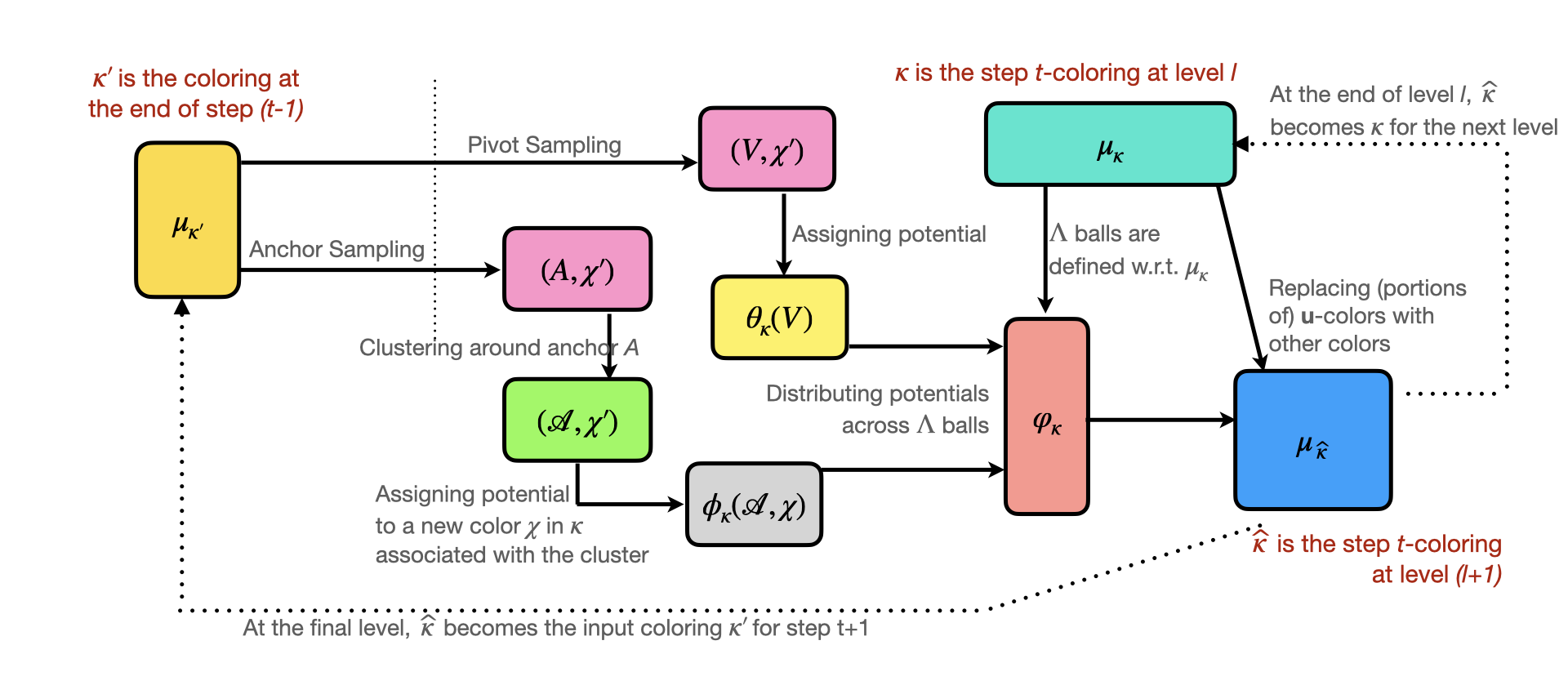
Figure 2: The flow of coloring intervals at level $l$

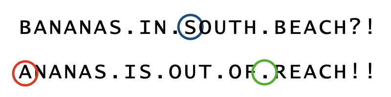
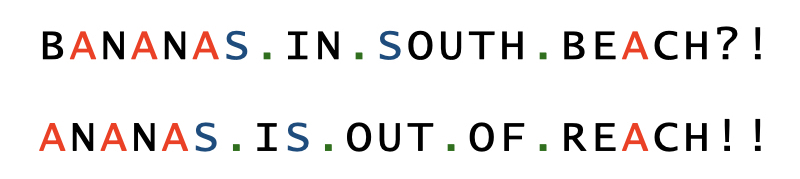
Figure 3: A step by step coloring example at level $l$. For simplification, all intervals start as ${\mathbf{u}}$-colored, we use one $\zeta=2$ radius, and omit the pivot sampling, density estimation, and thresholding processes.

A more detailed diagram and a step-by-step coloring example (both require more detailed technical setup) are presented, respectively, in Section 5, Figure 2 and Figure 3.

In each level $l\geq 1$, our goal is to color all intervals of density in a certain range $[n^{-\epsilon},1]\cdot d_{l}$, where $d_{l}\approx\tfrac{n/\lambda^{t}}{\beta^{l}}$, for $\beta=n^{\epsilon}$, as long as there are sufficiently many intervals of that density range overall. At level $l=0$, corresponding to the highest density for step $t$, we generate a 2-hop path for each pair of intervals in $A$’s cluster by “planting a star” in $G$; i.e., adding an edge between the anchor $A$ and each corresponding clustered interval $I$. Then, we mark (fraction of) $I$ as “already-matched” with the color $\bot$. In other levels, we color intervals found through extensions of clusters using $\varphi$.

The remaining case — “sparse” intervals that we did not yet color via an anchor cluster extension as above — will be addressed by the careful use of ${\mathbf{u}}$-color, described next. We remark that, at the end of step $t$, there may be left some pairs of small densities which we still could not color, and are left $\mathbf{u}$-colored, and we will show a bound on those as well. We now expand on the latter.

Controlling sparse sections: the ${\mathbf{u}}$-color.

In order to carry out the level-by-level coloring, we use the special color $\mathbf{u}$ (for un-colored). This color should be thought of as a “part” in the partition as well. At the beginning of a step, at level $l=0$, all (fractions of) intervals which are not “already-matched” are assigned the ${\mathbf{u}}$ color, and (fractions of) intervals are moved from ${\mathbf{u}}$-color to “standard” colors $\in[\lambda^{t}]$ as levels progress. The ${\mathbf{u}}$-color helps with three aspects. First, it provides a way to track sparse intervals which cannot yet be colored and hence left pending for future levels. Second, if some sparse sections of intervals are never colored in the current step, then these intervals will remain ${\mathbf{u}}$-colored (and hence, at the end of the current step, form a part that is also bounded in size). Third, and more nuanced, it allows us to “group together” sparse sections of intervals that are far apart (in their starting index).

In particular, such grouping of far intervals is done using the aforementioned “proximity balls”, formally defined via $\Lambda$-balls: $\Lambda_{\kappa}^{\zeta}(I)$ is the smallest interval ball around $I$ containing $\zeta\approx\beta^{l}$ $\mathbf{u}$-colored $\ell_{1}$-mass on both left and right of $I$. Note that $\Lambda$-balls can contain a significantly larger set of intervals than $\zeta$ (if the in-between intervals are mostly colored $\neq{\mathbf{u}}$). At the same time, the ball contains at most $2\zeta$ mass of $\mathbf{u}$-colored intervals, meaning that the potential $\phi(I)$ is distributed to a mass $\mu\leq 2\zeta$ of intervals, ensuring that, were $I$ to be “corrupted” (e.g., $\pi[I]=\bot$, or the pair $(I,\pi[I])$ happens to be already separated), we will incur only an $O(1)$ factor of total corrupted potential to $\varphi$’s of intervals in the $\Lambda$-ball of $I$.

To showcase the use of ${\mathbf{u}}$-color, consider again the running example introduced in Section 3.1. In the early steps $t$, our algorithm will first color the dense intervals (i.e., via clustering/proximity balls, at lower levels $l$), leaving the sparse sections mostly unaffected, all colored in ${\mathbf{u}}$ (during such early steps, the dense intervals are partitioned into progressively smaller parts while most of the sparse ones remain ${\mathbf{u}}$-colored). Now consider a step $t$ where the part sizes so far are $\lesssim n/\lambda^{t-1}\approx\Delta n$ and we sample $\gtrsim 1/\Delta$ anchors. At the lower levels $l$, the dense intervals will be partitioned further (continuing the process from the previous steps) and assigned a color $\chi\in[\lambda^{t}]$. However, when we reach the high levels $l$, and $\zeta\approx\beta^{l}=n^{\epsilon l}$ is close to $\Delta n$, some fraction of the sparse intervals will be clustered. Furthermore, since at that point the dense intervals are already colored (and have little ${\mathbf{u}}$-color), the $\Lambda$-balls around the clustered sparse intervals will be wide and cover most of the ${\mathbf{u}}$-colored sparse intervals. That allows us to finally partition the sparse intervals into smaller parts as well.

Keeping track of errors in analysis: Corruption.

To measure and bound errors, in particular, $\pi$-matched interval that are separated, we use a formal notion of corruption. First we define what it means for a (interval, color) pair to be corrupted. Below, $F\gg 1$ is a “distortion” factor (used for the non-PNA case), which one can think of being $F=2$ for now.

Definition 3.1 (Corrupted pairs).

Fix alignment $\pi\in\Pi$, interval $I\in\mathcal{I}$, distortion $F\geq 1$, and graph $G$ on $\mathcal{I}$. For a color $\chi\in\nu$, we say $(I,\chi)$ is a ($F,\pi,G,c,\kappa$)-corrupted pair if any of the following holds:

1. $\pi[I]=\bot$;

2. $\mathtt{ad}(I,\pi[I])>c$;

3. $\chi\neq\bot$ and $\mu_{\kappa}(I,\chi)>F\cdot\mu_{\kappa}(\pi[I],\chi)$; or

4. $\chi=\bot$ and $(I,\pi[I])$ are at hop-distance $>2$ in $G$.

For each interval $I\in\mathcal{I}$, we also define corruption parameter $\xi_{F}^{\kappa,\pi,G,c}(I)\in[0,1]$ as follows:

$$\xi_{F}^{\kappa,\pi,G,c}(I)=\sum_{\chi:(I,\chi)\text{ is }(F,\pi,G,c,\kappa)\text{-corrupted pair}}\mu_{\kappa}(I,\chi).$$ (1)

In particular, an interval $I$ is fully corrupted (in a coloring $\kappa$) if it does not have its $\pi$-matchable counterpart; and otherwise $I$ is corrupted by the total $\ell_{1}$ color-mass of $\mu_{\kappa}(I,*)$ where there is insufficient corresponding mass in $\mu_{\kappa}(\pi[I],*)$ (intuitively, the distribution of colors is too different). While our statements hold for any alignment in $\Pi$, we only care about a fixed optimal alignment $\pi$, a single graph $G=G_{w,c}$ and a fixed cost $c$. Hence, for ease of exposition, we say $I$ is $F$-corrupted and the corruption is $\xi^{\kappa}_{F}(I)\triangleq\xi^{\kappa,\pi,G,c}_{F}(I)$. Our main goal is to bound the total corruption $\xi^{\kappa}_{F}\triangleq\xi_{F}^{\kappa}(\mathcal{I})$, and in particular show it grows by at most a constant factor in any level/step. Our algorithm runs for a constant number of levels/steps, and hence finishes with corruption which is proportional to the number of intervals without a $\pi$-matchable counterpart (starting corruption), upper-bounded by $O(\tfrac{w}{c}\cdot\mathtt{ed}(x,y))$. Also, at the end of the interval matching algorithm, all intervals are “already matched”, i.e., all mass is on $\mu_{\kappa}(\mathcal{I},\bot)$, and hence the un-corrupted intervals have a 2-hop path to their $\pi$-match.

To bound the corruption growth, we also introduce the parameter $\rho(I)$, which measures the “local amount of corruption” of an ${\mathbf{u}}$-colored interval, based on the nearby corrupted intervals. In particular, $\rho(I)$ is defined for a $\Lambda$-ball around $I$ as the ratio of the corruption to the ${\mathbf{u}}$-mass inside the $\Lambda$-ball (formally defined in Section 6.1). One can observe that for any fixed $\zeta$ radius of $\Lambda$, the sum of $\rho$ over ${\mathbf{u}}$-colored intervals is proportional to the total sum of corruption.

Completing the algorithm under the perfect neighborhoods assumption (PNA).

Once we compute the palettes $\varphi$ of all intervals (as a function of the sampled anchors), we then use them to update $\mu$ for the next level. For illustrative purposes, we now complete the algorithm under the PNA, although our general algorithm will differ significantly from the PNA one. Recall that under PNA, all intervals are either at $\mathtt{ad}$-distance $\leq c$ or $\gg c$, and hence the intervals form equivalence classes according to their $c$-neighborhood.

Under PNA, we are guaranteed that the uncorrupted $\pi$-matchable pairs will get similar potentials —in fact, $\phi(I)$ and $\phi(\pi[I])$ are precisely equal (and non-zero whenever they are clustered by an anchor). More importantly, if we consider the $\varphi$ palettes of $I,\pi[I]$, which gather the contributions from clusters containing $I,\pi[I]$ in their proximity ball, then one can prove that (the average) $\ell_{1}$ distance between the two $\varphi$ palettes is bounded as a function of the “local corruption”, namely $\rho(I)$ and $\rho(\pi[I])$.

Using the $\ell_{1}$-distance property of $\varphi$, we can assign a single color $\chi\in\nu$ to each interval (i.e., $\mu_{\kappa}(I,*)$ has support one), obtaining disjoint partitions. To generate such a color (for each interval) we can use a random weighted min-wise hash function $h\sim\mathcal{H}$ for ${\mathbb{R}}^{\nu}$ (say, using [Cha02]) and use it to partition the vectors $\varphi(I,*)$ of all ${\mathbf{u}}$-colored intervals $I$. Specifically, sample a minhash $h:{\mathbb{R}}^{\nu}\to\nu$ and set the updated coloring to be $\mu_{\widehat{\kappa}}(I,h(\varphi(I)))\leftarrow 1$ (the rest are 0) for all $I$ for which $\mu_{\kappa}(I,{\mathbf{u}})=1$ at the end of the previous level.

For a glimpse of the analysis, recall that our overall goal is to make each part of the partition smaller (for runtime complexity) with only a constant-factor corruption growth (for correctness); also, we care only to partition areas with large mass of intervals with density in some range $[n^{-\epsilon},1]\cdot d_{l}$ (in a fixed level $l$). To control the size of parts, we cannot afford to assign the same color to too many intervals; hence we drop from $\varphi$ all colors of potential below some fixed threshold $o(n^{-\epsilon})$, ensuring that each color appears in the $\varphi$ palettes of at most $\tfrac{n^{1+O(\epsilon)}}{\lambda^{t-1}}$ intervals. For bounding the corruption, we note that minhash gives us a bound proportional to the Jaccard distance between $\varphi(I)$ and $\varphi(\pi[I])$, while the $\rho$ bound we have is in $\ell_{1}$ distance. Showing these bounds are close is where the $\mathbf{u}$-color plays a central role. First, consider an interval $I$ such that $\Omega(\epsilon)$ portion of its proximity ball $\Lambda$ is composed of intervals of density $\in[n^{-\epsilon},1]\cdot d_{l}$, where $\Lambda$ is of radius $\zeta$. Then the palette $\varphi(I)$ has $\ell_{1}$ mass $\Omega(\epsilon)$ whp after thresholding since: 1) some intervals in $\Lambda$ will be clustered whp (they are dense enough), and 2) once clustered, the generated potential is large enough to pass the threshold (since they are not too dense). In this case, we are done (without using the color ${\mathbf{u}}$): the Jaccard distance is proportional to the $\ell_{1}$ distance between $\varphi(I)$ and $\varphi(\pi[I])$, and hence the probability of separating $I$ from $\pi[I]$ is bounded by the “local corruption” (which overall is bounded by the total corruption). Second, consider the case when $1-o(\epsilon)$ portion of intervals in the $\Lambda$ ball are outside the aforementioned density range. Then we add mass to $\varphi(\cdot,{\mathbf{u}})$ of intervals in the ball $\Lambda$, filling it up to reach $\|\varphi(I)\|_{1}=\Omega(\epsilon)$ — this will increase the probability that such intervals are mapped (again) to ${\mathbf{u}}$ (this increases corruption by a factor $\leq 2$). This process also guarantees $\Lambda$ balls at the next level $l$ have $(1-o(\epsilon l))\cdot\zeta$ mass of sparse intervals, i.e., of density $\lesssim\tfrac{n/\lambda^{t}}{\beta^{l}}$. One can then prove that, after running this process for $\approx 1/\epsilon$ levels, the set of intervals corresponding to each color, including ${\mathbf{u}}$, is of size $\lesssim n/\lambda^{t}$ only.

Since we could not directly extend the minhash construction to the general non-PNA case, we do not present this construction in the paper, but rather use it as an intuition for its “robust” version as we describe next.

3.4 Imperfect neighborhoods

To eliminate the perfect neighborhood assumption (PNA), we must rely on the weaker form of transitivity instead, from the triangle inequality: $\mathcal{N}_{c}(I)\subseteq\mathcal{N}_{2c}(J)\subseteq\mathcal{N}_{3c}(I)$ for any $J\in\mathcal{N}_{c}(I)$. Note that the usual ideas to deal with such “weaker transitivity” do not seem applicable here. For instance, if we pick the threshold of “close” in the cluster construction to be uniformly random $\in[c,O(c)]$, there’s still a constant probability of separating $I$ from $\pi[I]$. One could instead apply the more nuanced metric random partitions, such as from [MN07], which would partition the metric $(\mathcal{I}_{w},\mathtt{ad}_{w})$ (thus putting us back into the perfect neighborhood assumption), with the probability of $I,\pi[I]$ ending up in the same part being $\geq n^{-\epsilon}$ — which has been useful in other contexts by repeating such partition $\approx n^{\epsilon}$ times. However, such a process results in a random partition retaining only $n^{1-\epsilon}$ $\pi$-matched pairs, which is not enough to reconstruct even those matched pairs (intuitively, the strings are “too corrupted”, as if the edit distance is $(1-o(1))\cdot n$), making it inapplicable for our algorithm (here again, this challenge would be more manageable if additive approximation were allowed). Overall, dealing with imperfect neighborhoods proved to be a substantial challenge for us, and we develop several first-of-a-kind tools specifically to deal with it.

Eventually, we still sample a cost $c_{i}$ from some ordered set $E_{c}=\{c_{1},c_{2},\ldots\}\subset[c,O(c)]$. Since we want that the cost $c_{i}$ satisfies that $\mathcal{N}_{c_{i}}(\mathcal{N}_{c_{i}}(I))\subseteq\mathcal{N}_{c_{i+1}}(I)$, we set $E_{c}$ of costs to be exponentially-growing, i.e., $c_{i}=\Theta(c)\cdot 3^{i}$. The formal definition is in Section 5.

Distortion Resilient Distance.

Relying purely on triangle inequality forces us to assign somewhat different potential scores to $I$ and $\pi[I]$, hence we will quantify the ratio between the two, referring to it as “distortion”.

While it may be tempting to try to keep the distortion to a constant, it turns out one cannot do that without introducing super-constant factor corruption growth (number of pairs with a large distortion), which is prohibitive for us. To control corruption, we allow the distortion (i.e., the multiplicative difference) between $\phi(I)$ and $\phi(\pi[I])$ for $\pi$-matchable pairs can be as high as $n^{\alpha}$ for some small constant $\alpha>0$. However, such a distortion makes it impossible to obtain a bound on $\ell_{1}$ distance between $\varphi$’s of a $\pi$-match, which is proportional to $\rho$. Instead, we deal with such distortion by employing a distortion resilient (robust) version of $\ell_{1}$.

Definition 3.2.

Fix $p,q\in{\mathbb{R}}^{k}_{+}$. We define the $F$-distortion resilient distance,

$$\operatorname{\mathtt{dd}}_{F}(p,q)=\sum_{i:p_{i}>F\cdot q_{i}}p_{i}$$

.

This function allows us to define and control corruption of (interval, color) pairs by differentiating distortion (which captures multiplicative errors) from corruption (which captures additive ones). As part of our analysis, we will show several basic properties of the $\operatorname{\mathtt{dd}}$ distance and develop $\operatorname{\mathtt{dd}}$-preserving soft-transformations, which will replace the hard thresholds from the minhash construction. Intuitively, $\operatorname{\mathtt{dd}}$ replaces the use of the $\ell_{1}$/Jaccard metric on the vectors $\phi$ and $\varphi$, which was a key enabler for using minhash under PNA. However, $\operatorname{\mathtt{dd}}$ is not a metric in any reasonable sense (it’s not even symmetric), rendering the minhash construction obsolete (e.g., it is unreasonable to expect any kind of LSH under $\operatorname{\mathtt{dd}}$).

Assigning potential to (interval, color) pairs.

Since maintaining equivalence classes is essential for our construction, we analyze pairs of interval and colors in $\mathcal{I}\times\nu$ (which, combinatorially, can be thought of as “fractions of intervals”). Thus, when we increase the $\phi$-potential of a clustered pair $(I,\chi^{\prime})$, we do so proportionally to its $\mu$ mass, meaning we set the potential to $\approx\mu(I,\chi^{\prime})\tfrac{n}{d\cdot\lambda^{t}}$. Similarly, splitting the $\phi$ potential to ${\mathbf{u}}$-colored-pairs in $\Lambda$ balls (i.e., assigning $\varphi$) is done in a pro-rated fashion, weighted according to respective $\mu(\cdot,{\mathbf{u}})$ masses.

Assigning ${\mathbf{u}}$ potential: pivot sampling.

Having so far discussed assigning of the non-${\mathbf{u}}$ colors in $\varphi$ of (fractions of) intervals, we now discuss how to assign ${\mathbf{u}}$-color in $\varphi_{\kappa}$ and, eventually, amended coloring $\mu_{\widehat{\kappa}}$. It may be tempting to merely subtract the assigned fraction of non-${\mathbf{u}}$-color from the ${\mathbf{u}}$-color mass, but this would result in additive errors (for the color ${\mathbf{u}}$), while $\operatorname{\mathtt{dd}}$ only allows for multiplicative distortion. In particular, we need ${\mathbf{u}}$ colors to agree up to a fixed distortion as well (to avoid more corruption), and hence we compute the new ${\mathbf{u}}$-color mass directly, via a different technique for explicitly measuring sparseness (which is the central purpose of ${\mathbf{u}}$-color). To accomplish this measurement, we developed a procedure called pivot sampling, which somewhat resembles the way we assign potentials for the non-${\mathbf{u}}$ colors. First, we downsample $\mathcal{I}\times\nu$ into a smaller set of pivots $\mathcal{V}$. Second, we approximate the density of each pivot in $\mathcal{V}$, for each possible cost in $E_{c}$, thus generating $\theta$-potential scores for each pivot. Third and last, such $\theta$ potential is split among the intervals in a $\Lambda$-ball in a similar fashion to how we split $\phi$, generating $\varphi(\cdot,{\mathbf{u}})$ potentials to intervals in sparse areas. This rather involved process, specific to dealing with imperfect neighborhoods, requires much care to be able to control: (1) corruption of $\mathbf{u}$-colors; (2) balance of palettes $\varphi$ (as we describe next); (3) sparsity guarantees for ${\mathbf{u}}$-color (part) at the end of the step $t$; and (4) computational efficiency of such sampling mechanism.

Amending a coloring in a level, using $\varphi$.

While $\operatorname{\mathtt{dd}}$ is a convenient analytical tool for bounding corruption, it lacks the basic properties to allow coordinated sampling between $\pi$-matchable pairs. Instead of sampling a color from $\varphi(I,*)$ (as was done under PNA), we add all colors in $\varphi(I,*)$ to the amended coloring $\mu_{\widehat{\kappa}}(I,*)$. To maintain a distribution of colors, we first combine $\varphi$ with pre-existing non-${\mathbf{u}}$-colors in $\mu$, and then normalize to have $\ell_{1}$-mass of $\mu_{\kappa}(I,{\mathbf{u}})$, i.e., what “remains to be colored”, thus ensuring that the overall amended $\mu_{\hat{\kappa}}(I,*)$ is a distribution. As in the PNA case, we need to bound extra corruption from normalization by ensuring that the palettes $\varphi$ have constant norms. While this analysis for the PNA solution is immediate (by construction), here, instead, we employ several combinatorial arguments that analyze mass of pairs with certain density over certain set of costs, eventually showing that in each level, we either add sufficient regular colors (corresponding to anchors/clusters) or $\mathbf{u}$-colors to all intervals while maintaining guarantees (1)–(4) above.

Controlling the growth of distortion.

Our arguments require that throughout the matching phase, the $\operatorname{\mathtt{dd}}$ distortion $F$ is bounded by $n^{o(\epsilon)}$ (in particular, to maintain control over the aforementioned soft-transformations). Many of our algorithmic steps generate extra distortion. To control both distortion (multiplicative error) and corruption (additive error), we parametrize maximum distortion $F=F(t,l)$ for each step/level a priori, and bound corruption $\xi_{F}^{\kappa}$ at each step/level using the pre-determined distortion parameter $F=F(t,l)$. The final approximation factor is a function of the maximum cost in $\tfrac{1}{c}E_{c}$ (which is further determined by the “base distortion” $F(1,0)=n^{\alpha}$), together with the corruption factor we show in each step. At the end of the day, a distortion $F$ bounded by $n^{o(\epsilon)}$ allows us to carry out the above arguments (i.e., some of the above arguments can only work under small distortion $F$).

3.5 The metrics $\mathtt{ad}_{w}$

We now briefly discuss the algorithm for computing the $\mathtt{ad}_{w}(I,J)$ distance, using oracle calls to $\mathfrak{D}_{w/\gamma}$ metric. This metric is used to compute distances when building the graph $G_{w}$, in the Interval Matching algorithm. Note that the latter makes $n^{1+O(\epsilon)}$ oracle calls to $\mathtt{ad}$, and hence the algorithm has to run in time $n^{O(\epsilon)}=\operatorname{poly}(\gamma)$.

Intuitively, $\mathtt{ad}_{w}(I,J)$ is meant to capture the following distance, which should be thought of as an extension of the edit distance over an alphabet with the metric $(\mathcal{I}_{w^{\prime}},\mathfrak{D}_{w^{\prime}})$ where $w^{\prime}=w/\gamma$:

$$\min_{\pi}\sum_{i\in[w]}\tfrac{1}{w^{\prime}}\mathfrak{D}_{w^{\prime}}(I+i,J+\pi(i)),$$

where $\pi$ ranges over all alignments of indexes of $I$ to indexes of $J$. One can show that essentially, if $\mathfrak{D}(I,J)=\mathtt{ed}(I,J)$, then, for $I=X_{i,w},J=Y_{j,w}$, the above distance is between $\Omega(\mathtt{ed}(X_{i,w},Y_{j,w}))$ and $O(\mathtt{ed}(X_{i,2w},Y_{j,2w}))$.

However, this distance function is hard to compute fast: not only it is as hard as computing edit distance on $w$-length strings, but even linear time (in $w\gg\operatorname{poly}(\gamma)$) is too much for us. In particular, it does not use the fact that $\mathfrak{D}_{w^{\prime}}(I+i,J+\pi(i))$ captures the information of blocks of length $w^{\prime}$. Hence, it is natural to approximate the above by considering a “rarefication” of the above sum as follows:

$$\min_{\pi}\sum_{i\in[\gamma]}\tfrac{1}{w^{\prime}}\mathfrak{D}_{w^{\prime}}(I+iw^{\prime},J+\pi(iw^{\prime})).$$ (2)

However, the latter will not satisfy the triangle inequality — which is crucial in the Interval Matching Algorithm — and in fact is not even symmetric: e.g., if the optimal $\pi(i)=i+1$, the $\mathtt{ad}_{w}(J,I)$ would be using $\mathfrak{D}$ on completely different arguments. This is especially an issue since $\mathfrak{D}$ may substantially over-estimate $\mathtt{ed}$ on some of the pairs (and hence “shift by one” can change the distance a lot).

Indeed, ensuring triangle inequality is the main challenge for defining and computing $\mathtt{ad}_{w}$ here. We manage to define an appropriate distance $\mathtt{ad}$, satisfying triangle inequality for “one scale only” metrics $\mathtt{ad}_{w,c}$, designed for distances in the range $\approx[c,\gamma c]$, which turns out to be enough for the Interval Matching algorithm.

First, we note that we have two different algorithms, corresponding to two distinct distance formulations: (i) for large distance regime, where $c>w/\gamma$; and (ii) for small distance regime, where $c\leq w/\gamma$. The reason there’s a big difference between the two cases is that when $c>w/\gamma$, the alignment $\pi$ may have a large displacement $|i-\pi(i)|\geq w/\gamma$, bigger than the length of “constituent” intervals for which we have the base metric $\mathfrak{D}_{w^{\prime}}$. Hence, for the “large distance” regime, when $c\geq w/\gamma$, we uses a slightly different (and simpler) algorithm that runs in time $\approx\operatorname{poly}(w/c)$, and hence is only good when $c$ is sufficiently large.

Finally, we sketch the harder, $\operatorname{poly}(\gamma)$-time algorithm, for not-so-large $c$. The idea is to allow alignment shifts in both intervals. More formally, let $T=\gamma^{3}$ and let ${\mathcal{A}}$ be the set of functions $A=(A_{x},A_{y})$ where $A_{x},A_{y}:[-\gamma,\gamma]\rightarrow\{0,1,\ldots,T-1\}$ are non-decreasing functions with $A_{x}[-\gamma]=A_{y}[-\gamma]=0$ and $A_{x}[\gamma]=A_{y}[\gamma]$. We define the distance $\mathtt{ad}_{w,c}(I,J)$, to be, where $\theta$ is essentially $\approx c/w$ and $\mathfrak{S}_{i}=\{0,1,\ldots,3T-A_{x}[i]-A_{y}[i]-1\}$:

$$\mathtt{ad}_{w,c}(I,J)\triangleq\min_{A\in{\mathcal{A}}}$$

$$\left(A_{x}[\gamma]+A_{y}[\gamma]\right)\theta w^{\prime}+\sum_{i\in[-\gamma,\gamma)}\tfrac{1}{T}\sum_{\Delta\in\mathfrak{S}_{i}}\mathfrak{D}_{w^{\prime}}\left(I+w^{\prime}(i+\theta(\Delta+A_{x}[i])),J+w^{\prime}(i+\theta(\Delta+A_{y}[i]))\right).$$

Intuitively, ignoring $\Delta$-sum (i.e., think $\Delta=0$), we obtain an alignment of $I$ to $J$ where the starting positions (of $w^{\prime}$-length intervals) are close to multiples of $w^{\prime}$ in both strings (as opposed to only one string, as in Eqn. (2)). While allowing such an alignment is enough for ensuring symmetry, it is still not enough to ensure triangle inequality. Consider intervals $I,J,K\in\mathcal{I}$ where we want to guarantee that $\mathtt{ad}(I,K)\leq\mathtt{ad}(I,J)+\mathtt{ad}(J,K)$. Apriori, there is no way to ensure an optimal alignment between $\mathtt{ad}(I,J)$ and $\mathtt{ad}(J,K)$ will use the same shifts and hence makes it hard to offset the distance of large blocks in $\mathtt{ad}(I,K)$. To solve the inconsistencies between the shifts, we use the $\Delta$-sum over all possible shifts (this is yet another instance of “averaging it out”). The last definition can also be computed in $\operatorname{poly}(\gamma)$ time by a standard dynamic programming.

Nonetheless, the following issue remains: think of the case when $\mathtt{ad}(I,J)$ and $\mathtt{ad}(J,K)$ use the maximally-allowed values of the alignment (namely $\gamma^{2}$), in which case $\mathtt{ad}(I,K)$ cannot use the natural composition of the two alignments (since it’s out of bounds). To solve this issue, we upper bound each $\mathtt{ad}_{w,c}$ with a maximal value $\gg c$ (which solves the triangle inequality issue), and define the (non-metric) distance $\mathtt{ad}_{w}(\cdot,\cdot)$ as the summation over all costs $c\in S_{w}$ which can be upper-bounded by $\mathtt{ad}_{w,c}$ (formal definition in section 9).

Finally, we remark that, at the end of the day, we cannot guarantee a per-pair upper bound on $\mathtt{ad}(I,J)$, but only on average, and only when comparing $X_{i,w}$ against $Y_{\pi(i),w}$ (although the triangle inequality is true everywhere). This is, nonetheless, just enough for estimating $\mathtt{ed}(x,y)$.

4 Top Level Algorithm

We now describe our “top-level” algorithm. We assume here that the first $(1-o(1))n$ positions of $x$ and $y$ are equal; we can remove this assumption by padding $x,y$ with some fixed unique character $, increasing the size of $x,y$ by a factor of, say, $O(\log n)$.

Our algorithm consists of $\log_{\gamma}n$ iterations, where $\gamma=n^{\epsilon}$. For each $w=\gamma^{i}$, $i\in[\log_{\gamma}n]$, we construct the metric $(\mathcal{I}_{w},\mathfrak{D}_{w})$, which align approximates the metric $(\mathcal{I}_{w},\mathtt{ed}_{w})$ (see Def. 2.3). Each iteration consists of two components: the alignment distance algorithm, and the interval matching algorithm, described in later sections. Below we assume that $n$ is a power of $\gamma$, which is without loss of generality (as we can increase $n$ appropriately by padding the strings).

Alignment Distance algorithm.

Assuming oracle access to $(\mathcal{I}_{w/\gamma},\mathfrak{D}_{w/\gamma})$, the metric constructed at the previous iteration, our alignment algorithm is an oracle for computing the distance $\mathtt{ad}_{w}(\cdot,\cdot)$ on $w$-length intervals. In fact, we have $O(\log n)$ such distance measures, $\mathtt{ad}_{w,c}$, one for each target cost scale $c\in S_{w}=\{1,2,4,\ldots w\}\cup\{1/2,1/4,\ldots,1/2n\}$. Each such function $\mathtt{ad}_{w,c}(\cdot,\cdot)$ evaluation is an edit-distance-like dynamic programming of size $\operatorname{poly}(\gamma)$, and overall can be computed using $\operatorname{poly}(\gamma)=n^{O(\epsilon)}$ time and oracle calls to $\mathfrak{D}_{w/\gamma}$.

Note that this algorithm does not run directly, but instead is used as an oracle inside the matching algorithm described next.

Interval Matching algorithm.

We construct a weighted graph $G_{w}$ on $\mathcal{I}_{w}$, such that the shortest path distance in $G_{w}$ approximates the $\mathtt{ad}_{w}$ distance on intervals. Again, this won’t be achieved for all pairs of intervals, but only for interval pairs that “matter”, i.e., that are in an optimal alignment for $\mathtt{ed}(x,y)$. The graph $G_{w}$ is the union of edges of the graphs $G_{w,c}$, for $c\in S_{w}$, each of them align approximating $\mathtt{ad}_{w,c}$ at “scale $c$”. Constructing the graphs $G_{w,c}$ is the heart of the matching algorithm.

Once we have the graph $G_{w}$, we build a fast distance oracle data structure on it, using the $\ell_{\infty}$ embedding of [Mat96], and whose output is the desired metric $\mathfrak{D}_{w}$. Overloading the notation, we call $\mathfrak{D}_{w}$ both the distance oracle data structure as well as the metric it produces. In particular, [Mat96] shows how one can embed any $n$-point metric into $\ell_{\infty}$ of dimension $d=O(\tfrac{1}{\epsilon}n^{\epsilon}\log n)$ while incurring $O(1/\epsilon)$ distortion only. Once we have such an embedding, we can compute distance between two points by evaluating $\ell_{\infty}$ distance in dimension $d$. Furthermore the embedding itself can be computed by running $d$ single-source shortest path (SSSP) computations. Hence, we obtain the following Theorem 4.1 as an immediate corollary of [Mat96] together with a standard $\tilde{O}(m)$-time SSSP algorithm.

Theorem 4.1 (corollary of [Mat96]).

For any constant $\epsilon>0$, given any weighted graph $G$ on $n$ nodes and $m$ edges, we can build a distance oracle data structure with the following properties:

• supports distance queries: given $u,v$, output $\mathfrak{D}_{G}(u,v)$ which is a $O(1/\epsilon)$-factor approximation to the shortest path distance between $u,v$ in the graph;

• $\mathfrak{D}_{G}(u,v)$ is a ($n$-point) metric;

• runtime per query is $\tilde{O}_{\epsilon}(n^{\epsilon})$;

• data structure uses $\tilde{O}_{\epsilon}(n^{1+\epsilon})$ space, and pre-processing time is $\tilde{O}_{\epsilon}(mn^{\epsilon})$.

Top-level algorithm

is described in Algorithm 1. At the beginning, when $w=\gamma$, we use the metric $(\mathcal{I}_{1},\mathfrak{D}_{1})$, which is just the metric on all positions in $x$ and $y$, where two positions are at distance 0 iff the positions contain the same character, and 1 otherwise. At the end, when $w=n$, we can extract the distance between $x$ and $y$, which is our final approximation. The algorithm MatchIntervals, described in Section 5, returns an unweighted graph $G_{w,c}$. The full graph $G_{w}$ for the scale $w$, is obtained by union of the graph edges of $G_{w,c}$ each scaled by $C_{m}c$, over all $c\in S_{w}$, together with some extra edges.

Algorithm 1 EstimateEditDistance$(x,y,\epsilon,n)$

function EstimateEditDistance($x,y,\epsilon,n$)

     Fix $C_{m}$ to be the constant from Theorem 4.2.

     $\gamma\leftarrow n^{\epsilon}$.

     $\mathfrak{D}_{1}$ is a data structure that, given two positions into $x$ and/or $y$, outputs 0 iff the characters in those positions are equal and 1 otherwise.

     for $w\in\{\gamma,\gamma^{2},\ldots,n\}$ do

         Let $\mathcal{X}_{w},\mathcal{Y}_{w}$ be sets of all $w$-length intervals on $x$-axis and $y$-axis respectively, with $\mathcal{I}_{w}=\mathcal{X}_{w}\cup\mathcal{Y}_{w}$.

         for  $c\in S_{w}$  do

              $G_{w,c}\leftarrow\textsc{MatchIntervals}(\mathfrak{D}_{w/\gamma},c)$.

         end for

         $G_{w}\leftarrow\cup_{c\in S_{w}}C_{m}\cdot c\cdot G_{w,c}$ and add edges $(X_{i,w},X_{i+1,w}),(Y_{i,w},Y_{i+1,w})$ with unit cost for all $i$.

         $\mathfrak{D}_{w}\leftarrow$ data structure from Theorem 4.1 on graph $G_{w}$ for approximation $10/\epsilon$.

     end for

     return $\mathfrak{D}_{n}(X_{i,n},Y_{i,n})$ for a randomly chosen $i\in[n]$.

end function

4.1 Main guarantees

The guarantees of the algorithm follow from the following two central theorems.

Theorem 4.2 (MatchIntervals; see Sections 5, 6, 7, 8).

Fix $\epsilon>0$, $w,n\in{\mathbf{N}}$, and cost $c\in S_{w}$. Suppose $(\mathcal{I}_{w},\mathtt{ad}_{w,c})$ is a metric, for which we have query access running in time $T_{\mathtt{ad}}$. Then, the algorithm MatchIntervals builds an undirected graph $G_{w,c}$, over intervals $\mathcal{I}_{w}$, such that:

1. For all edges $(I,J)\in G_{w,c}$, we have $\mathtt{ad}_{w,c}(I,J)\leq C_{m}\cdot c$, where $C_{m}=C_{m}(\epsilon)$ is a constant.

2. For any alignment $\pi\in\Pi$, with high probability: $|\{i\mid\operatorname{dist}_{G_{w,c}}(X_{i,w},Y_{\pi(i),w})>2\}|\leq C_{m}\cdot|\{i\mid\mathtt{ad}_{w,c}(X_{i,w},Y_{\pi(i),w})>c\}|$, where $\operatorname{dist}_{G_{w,c}}$ is the hop-distance in ${G_{w,c}}$.

3. The runtime of the algorithm is $O(T_{\mathtt{ad}}\cdot n^{1+O(\epsilon)})$ whp.

As described above, using the algorithm from the above theorem, we build a graph $G_{w}$, which is the union of scale graphs $G_{w,c}$. Then we take $\mathfrak{D}_{w}$ to be the fast distance oracle of the shortest path on the graph $G_{w}$, using Theorem 4.3.

Next theorem says that, given access to $\mathfrak{D}_{w/\gamma}$, we can compute $\mathtt{ad}_{w,c}(I,J)$ for any two intervals $I,J\in\mathcal{I}$, which corresponds to the “natural extension” of $\mathfrak{D}$ from length-$w/\gamma$ to length-$w$ substrings.

Theorem 4.3 (alignment distance $\mathtt{ad}$; see Section 9).

Fix $w$ and $w^{\prime}=w/\gamma$, and suppose we have a data structure for a metric $\mathfrak{D}_{w^{\prime}}$ that $C$-align-approximates $\mathtt{ed}$ for some constant $C\geq 1$, while also $\mathfrak{D}_{w^{\prime}}(X_{i,w^{\prime}},X_{i+1,w^{\prime}})\leq C$ for all $i\in[n]$ (and same for $Y$ intervals). Then, for any $c\in S_{w}$, the algorithm from Section 9 defines a function $\mathtt{ad}_{w,c}(\cdot,\cdot)$ on $\mathcal{I}_{w}\times\mathcal{I}_{w}$ with the following properties:

1. $(\mathcal{I}_{w},\mathtt{ad}_{w,c})$ is a metric;

2. For all $X_{i},Y_{j}\in\mathcal{I}_{w}$, $\mathtt{ad}_{w,c}(X_{i},Y_{j})\geq\min\{\mathtt{ed}_{w}(X_{i},Y_{j}),c\sqrt{\gamma}\}$;

3. Define $\mathtt{ad}_{w}(X_{i},Y_{j})\triangleq\sum_{c\in S_{w}}c\cdot{\mathbb{1}}\left[{\mathtt{ad}_{w,c}(X_{i},Y_{j})\geq c}\right]$. Then, $\mathtt{ad}_{w}$ $O(C)$-align-approximates $\mathtt{ed}$.

4. For all $I,J\in\mathcal{I}_{w}$, $\mathtt{ad}_{w,c}(I,J)$ can be computed using $\tilde{O}(\gamma^{O(1)})$ time and queries to $\mathfrak{D}_{w^{\prime}}$.

We remark that $\mathtt{ad}_{w}$ is not guaranteed to be a metric, which is the reason why we use $\mathtt{ad}_{w,c}$ in the theorem statement. Also, the algorithm from Section 9 requires no further preprocessing.

4.2 Proof of Theorem 1.1

To prove Theorem 1.1, we just combine the above two theorems, 4.2 and 4.3. In particular, the inductive hypothesis is that, for $w=\gamma^{i}$, where $i\in[\log_{\gamma}n]$, the distance oracle data structure $\mathfrak{D}_{w}$ outputs a metric $\mathfrak{D}_{w}$ with the following properties, for some constant $C_{w}=C(\epsilon,\log_{\gamma}w)$, whp:

1. $\mathfrak{D}_{w}$ $C_{w}$-align-approximates $\mathtt{ed}$;

2. $\mathfrak{D}_{w}(X_{i,w},X_{i+1,w})\leq 10/\epsilon$ (and same for $Y$ intervals).

Base case: for $w=1$, this is immediate by construction of $\mathfrak{D}_{1}$.

Now assume the inductive hypothesis for $w^{\prime}=w/\gamma$ and we need to prove it for $w$. By inductive hypothesis, $\mathfrak{D}_{w^{\prime}}$ satisfies hypothesis of Theorem 4.3, and hence we can apply it to obtain an oracle query to metrics $\mathtt{ad}_{w,c}$; each oracle query takes $O(\gamma^{O(1)})$ time. Let $\pi$ be optimizer for $\min_{\pi}\sum_{i}\mathtt{ad}_{w}(X_{i,w},Y_{\pi(i),w})$ (guaranteed to align-approximate $\mathtt{ed}$).

Define $\tau(\cdot,\cdot)$ to be the distance in the graph $G_{w}$ constructed in the algorithm. We will prove below that $\tau$ is a metric satisfying the above properties. Hence, once we build a fast distance oracle $\mathfrak{D}_{w}$ on the graph $G_{w}$ (using Theorem 4.1), its output metric $\mathfrak{D}_{w}$ satisfies $\tau\leq\mathfrak{D}_{w}\leq O(\tau/\epsilon)$, and hence the inductive hypothesis.

To prove the first property of the inductive hypothesis, consider any two intervals $I,J$, and the shortest path $v_{1},\ldots v_{k}$ between them, where $v_{1}=I$ and $v_{k}=J$. We have that $(v_{i},v_{i+1})$ is an edge in some graph $G_{w,c_{i}}$, or is an extra edge of cost $1$; call $E$ the set of the latter $i$’s. Hence the cost $\tau(I,J)=\sum_{i\not\in E}C_{m}c_{i}+|E|$. For $i\not\in E$, by Theorem 4.2 and Theorem 4.3, we have that $C_{m}c_{i}\geq\mathtt{ad}_{w,c_{i}}(v_{i},v_{i+1})\geq\mathtt{ed}_{w}(v_{i},v_{i+1})$ (note that the other part of the min cannot happen as $C_{m}\ll\sqrt{\gamma}$). Also, for $i\in E$, we have that $1=\tau(v_{i},v_{i+1})\geq\mathtt{ed}_{w}(v_{i},v_{i+1})$ as $\mathtt{ed}_{w}(X_{i},X_{i+1})\leq 1$ (and same for $Y$’s). Hence $\mathfrak{D}(I,J)\geq\tau(I,J)=C_{m}\sum_{i\not\in E}c_{i}+|E|\geq\mathtt{ed}_{w}(v_{1},v_{2})+\ldots+\mathtt{ed}_{w}(v_{k-1},v_{k})\geq\mathtt{ed}_{w}(I,J)$.

Next, we note that $\tau(I,J)$ is upper bounded by $2C_{m}\min_{c\in S_{w}}c+\sum_{c\in S_{w}}4\cdot C_{m}c\cdot{\mathbb{1}}\left[{\operatorname{dist}_{G_{w,c}}(I,J)>2}\right]=C_{m}/n+4C_{m}\sum_{c\in S_{w}}c\cdot{\mathbb{1}}\left[{\operatorname{dist}_{G_{w,c}}(I,J)>2}\right]$. Hence:

$$\sum_{i\in[n]}\tau(X_{i,w},Y_{\pi(i),w})\leq C_{m}+4C_{m}\sum_{c\in S_{w}}\sum_{i\in[n]}c\cdot{\mathbb{1}}\left[{\operatorname{dist}_{G_{w,c}}(X_{i,w},Y_{\pi(i),w})>2}\right].$$

For fixed $c\in S_{w}$, we have that, by Theorem 4.2:

$$\sum_{i\in[n]}{\mathbb{1}}\left[{\operatorname{dist}_{G_{w,c}}(X_{i,w},Y_{\pi(i),w})>2}\right]\leq C_{m}\cdot\sum_{i}{\mathbb{1}}\left[{\mathtt{ad}_{w,c}(X_{i,w},Y_{\pi(i),w})>c}\right].$$

Therefore,

$$\sum_{i\in[n]}\tau(X_{i,w},Y_{\pi(i),w})\leq O\left(1+\sum_{c\in S_{w}}\sum_{i\in[n]}c\cdot{\mathbb{1}}\left[{\mathtt{ad}_{w,c}(X_{i,w},Y_{\pi(i),w})>c}\right]\right)\leq O\left(1+\sum_{i\in[n]}\mathtt{ad}_{w}(X_{i,w},Y_{\pi(i),w})\right).$$

Since $\pi$ is the optimizer for the right-hand-side, using Theorem 4.3 again, together with the inductive hypothesis for $w^{\prime}=w/\gamma$, we conclude (where constant depends on $\epsilon$ and $\log_{\gamma}w$):

$$\sum_{i\in[n]}\mathfrak{D}_{w}(X_{i,w},Y_{\pi(i),w})\leq O\left(\sum_{i\in[n]}\tau(X_{i,w},Y_{\pi(i),w})\right)\leq O\left(1+\sum_{i\in[n]}\mathtt{ad}_{w}(X_{i,w},Y_{\pi(i),w})\right)$$

$$\leq O\left(\min_{\pi}\sum_{i}\mathtt{ed}_{w}(X_{i,w},Y_{\pi(i),w})\right),$$

since we can assume wlog that $\mathtt{ed}(x,y)\geq 1$ (checking the opposite is immediate), thus completing the proof of the inductive hypothesis.

The second property is immediate by construction of the graph $G_{w}$ and the fact that approximation of the distance oracle $\mathfrak{D}_{w}$ is taken to be $10/\epsilon$.

Now we argue that the final output produced by the top-level algorithm is a constant factor approximation. Consider the $\mathfrak{D}_{w}$ guarantees for $w=n$, and fix the minimizing $\pi$, and constant $C_{n}=C_{w}$. For a random index $i\in[n]$, with probability at least $0.9$, we have that: 1) $i\in[1,n-o(n)]$, 2) $\pi(i)\neq\bot$, and $\mathfrak{D}(X_{i,n},Y_{\pi(i),n})\leq O(C_{n})\cdot\mathtt{ed}(x,y)$. Furthermore note that $|i-\pi(i)|\leq C_{n}\cdot\mathtt{ed}(x,y)$, and hence, $\mathfrak{D}(X_{i,n},Y_{i,n})\leq\mathfrak{D}(X_{i,n},Y_{\pi(i),n})+\tfrac{10}{\epsilon}\cdot|i-\pi(i)|\leq O(C_{n}/\epsilon)\cdot\mathtt{ed}(x,y)$. Also, since $i\leq n-o(n)$, we have that $\mathfrak{D}(X_{i,n},Y_{i,n})\geq\mathtt{ed}(X_{i,n},Y_{i,n})=\mathtt{ed}(x,y)$.

Concluding, the algorithm produces a $O(C_{n}/\epsilon)$ approximation to $\mathtt{ed}(x,y)$, with probability $\geq 0.9$. Note that $C_{n}$ is a constant, depending on $\epsilon$, as we have only a constant number of iterations, each incurring a constant factor approximation.

The runtime guarantee follows from time guarantees of Theorems 4.1, 4.2, and 4.3. In particular, by Theorems 4.1 and 4.3, the runtime $T_{\mathtt{ad}}$ is $\tilde{O}(\gamma^{O(1)})\cdot n^{O(\epsilon)}=n^{O(\epsilon)}$. Hence runtime in the matching algorithm, for every fixed $w$, is $n^{1+O(\epsilon)}$. Thus the graph $G_{w}$ has size $n^{1+O(\epsilon)}$ and the preprocessing time of Theorem 4.1 is $n^{1+O(\epsilon)}$ as well. Overall, we have a constant number of $w$’s to consider, and thus we obtain a runtime of $n^{1+O(\epsilon)}$.

5 Interval Matching Algorithm

In this section we describe our main interval matching algorithm, used to prove Theorem 4.2. The correctness and runtime complexity analysis will follow in Sections 6 and 8 respectively.

Our matching algorithm iterates over a constant number of steps $t$, each iterating over a constant number of levels $l$. The following MatchIntervals algorithm is the main loop over steps. We note that, in order to maintain high probability statements, in each step we output $O(\log n)$ output coloring for each input coloring.

Algorithm 2 Matching Algorithm

Input:    Base cost ${\mathfrak{c}}$
      Output: A matching graph $G=G_{w,{\mathfrak{c}}}$.

1:function MatchIntervals(${\mathfrak{c}}$)

2:     $\mathit{K}_{0}\leftarrow$ {initialize a new coloring of a single color ${\mathbf{u}}$ assigned with mass 1 to all $\mathcal{I}$}.

3:     $G\leftarrow$ unweighted and undirected graph with nodes $I\in\mathcal{I}_{w}$ and no edges.

4:     for $t=1,2,\ldots$ do

5:         $\mathit{K}_{t}\leftarrow\emptyset$.

6:         for $\{\kappa^{\prime}\in\mathit{K}_{t-1}\mid\mu_{\kappa^{\prime}}(\mathcal{I},\nu\setminus\bot)>0\}$ do

7:              for $O(\log n)$ times do

8:                  $(G,\mathit{K}_{t})\leftarrow(G,\mathit{K}_{t})\uplus$$\textsc{MatchStep}({\mathfrak{c}},\kappa^{\prime},t)$.

9:              end for

10:         end for

11:         break if $\mathit{K}_{t}=\emptyset$.

12:     end for

13:     return $G$.

14:end function

It remains to describe the MatchStep algorithm, which iterates over a constant number of levels. In each such level, the algorithm updates the coloring $\kappa$ under construction, to obtain the “amended” coloring $\widehat{\kappa}$, while also using the “step input coloring” $\kappa^{\prime}$, obtained at the end of the previous step. At the end of the iteration over the levels, the algorithm MatchStep produces a number of edges to add to the graph as well as a coloring. The pseudo-code for MatchStep is presented in Alg. 8, after a detailed description of the mechanisms and subroutines of MatchStep.

5.1 Components of MatchStep: setup and notations

We first introduce basic notions used in our algorithm. To help the reader keep track of the many definitions and notations, we summarize them in Table 1 and Table 2 for quick reference (the latter table is in Section 6). To avoid confusion, we use ${\mathfrak{c}}$ to denote $c$ from the theorem statement. Also, to simplify notation, we refer to the oracle $\mathtt{ad}_{w,{\mathfrak{c}}}$ simply as $\mathtt{ad}$. Note that $\mathtt{ad}$ algorithm uses the data structure $\mathfrak{D}_{w/\lambda}$, which we assume all our algorithms in this section have access to.

The set of costs $E_{\mathfrak{c}}$.

For each fixed base cost ${\mathfrak{c}}\in S_{w}$, we use a fixed set of costs $E_{\mathfrak{c}}\subset{\mathfrak{c}}\cdot[1,O(1)]$. The set $E_{\mathfrak{c}}$ is defined as $\{c_{1},c_{2},\ldots c_{1/\eta}\}$, where $c_{i}=\tfrac{{\mathfrak{c}}}{\epsilon\cdot\alpha}\cdot 3^{i}$, for small constants $\alpha,\eta>0$ (to be fixed later).

Colorings.

Recall our definition of coloring $\kappa$ over color-set $\nu$ as a mapping from intervals to distribution of colors in $\nu$, denoted by $\mu_{\kappa}:\mathcal{I}\times\nu\rightarrow[0,1]$.

Our construction analyzes pairs of intervals and colors $(I,\chi)\in\mathcal{I}\times\nu$. For a set ${\mathcal{R}}\subseteq\mathcal{I}\times\nu$ of (interval, color) pairs, $\mu_{\kappa}({\mathcal{R}})$ is the $\ell_{1}$ mass of colors in ${\mathcal{R}}$, i.e. $\mu_{\kappa}({\mathcal{R}})\triangleq\sum_{(I,\chi)\in{\mathcal{R}}}\mu_{\kappa}(I,\chi)$. We often use the shorthand pairs when referring to (interval, color) pairs.

We use colorings to partition $\mathcal{I}$ into smaller (overlapping) parts. For a color $\chi$, we denote its part by $\mathcal{P}_{\kappa}^{\chi}\triangleq\{I\in\mathcal{I}\mid\mu_{\kappa}(I,\chi)>0\}$.

Finally, we equip each $\mu_{\kappa}$ with a data structure that allows efficient sampling from it (Theorem 8.1). The reader should henceforth consider that sampling takes time proportional to the output size, up to $\operatorname{poly}(\log n)$ factors.

Proximity balls $\Lambda$.

For coloring $\kappa$ and $\zeta\in{\mathbf{N}}$, we define $\Lambda_{\kappa}^{\zeta}(I)$ as the largest interval ball around $I$ containing at most $\zeta$ $\mathbf{u}$-colored $\ell_{1}$-mass on each of left and right of $I$, where $\mu_{\kappa}(I,{\mathbf{u}})$ is counted on both sides. An exception to the above is for $\zeta=0$, when $\Lambda_{\kappa}^{0}(I)=\{I\}$. We note that for all $I\in\mathcal{I}$, $\zeta\geq 1$, we have $\mu_{\kappa}(\Lambda_{\kappa}^{\zeta}(I),{\mathbf{u}})\leq 2\zeta$.

Extending the data structure for $\mu_{\kappa}$ above, we also use the data structure from Theorem 8.2 to be able to compute the boundaries of any $\Lambda_{\kappa}^{\zeta}(I)$, given $I,\zeta$, in $\operatorname{poly}(\log n)$ time.

Interval and Pair densities.

For $I\in\mathcal{I}$, $\kappa$, color $\chi\in\nu$ and interval set ${\mathcal{S}}\subseteq\mathcal{I}$, we define a density parameter $\operatorname{{d}}_{\kappa}(I,\chi,{\mathcal{S}})_{\hat{c}}\triangleq\mu_{\kappa}(\mathcal{N}_{\hat{c}}(I)\cap{\mathcal{S}},\chi)$. We use the shorthand $\operatorname{{d}}_{\kappa}(I,\chi)_{\hat{c}}\triangleq\operatorname{{d}}_{\kappa}(I,\chi,\mathcal{I})_{\hat{c}}$. We also define the density vector $\operatorname{{d}}_{\kappa}(I,\chi,{\mathcal{S}})\in{\mathbb{R}}_{+}^{E_{\mathfrak{c}}}$ such that:

$$\operatorname{{d}}_{\kappa}(I,\chi,{\mathcal{S}})\triangleq[\operatorname{{d}}_{\kappa}(I,\chi,{\mathcal{S}})_{\hat{c}}]_{\hat{c}\in E_{\mathfrak{c}}}$$

We also define relative density as follows:

Definition 5.1 (Relative density.).

Fix $I\in\mathcal{I}$, $\kappa$, color $\chi$ and an interval set ${\mathcal{S}}\ni I$. The relative density $\operatorname{{rd}}_{\kappa}(I,\chi,{\mathcal{S}})\in[1,\infty)^{E_{\mathfrak{c}}}$ is the density of $I$ w.r.t. each cost $\hat{c}\in E_{\mathfrak{c}}$, divided by such density restricted to the set ${\mathcal{S}}$, i.e., $\operatorname{{rd}}_{\kappa}(I,\chi,{\mathcal{S}})\triangleq\operatorname{{d}}_{\kappa}(I,\chi)\oslash\operatorname{{d}}_{\kappa}(I,\chi,{\mathcal{S}})$.

By convention, we set the relative density of empty colors to 1 (or $\infty$ if empty in ${\mathcal{S}}$ only). Note that $\operatorname{{rd}}_{\kappa}(I,\chi,{\mathcal{S}})\geq 1$ and is monotonically decreasing in ${\mathcal{S}}$. Both are important properties that will be used when we bound density mass in “growing balls of intervals”.

Table 1: Summary of matching algorithm setup notations.

Notation	Description
Intervals
${\mathcal{X}},{\mathcal{X}}_{w}$	space of all $w$-length intervals of $x$.
${\mathcal{Y}},{\mathcal{Y}}_{w}$	space of all $w$-length intervals of $x$.
$\mathcal{I},\mathcal{I}_{w}$	space of all $w$-length intervals $={\mathcal{X}}\cup{\mathcal{Y}}$.
Distances
$(\mathcal{I},\mathtt{ad}_{w}),(\mathcal{I},\mathtt{ad}_{w,{\mathfrak{c}}})$	alignment-distances. $\mathtt{ad}_{w}$ align-approximates $\mathtt{ed}$. $\mathtt{ad}_{w,{\mathfrak{c}}}$ is a metric.
$({\mathbb{R}}_{+}^{d},\operatorname{\mathtt{dd}}_{F})$	distortion resilient distance for $F>1$. $\operatorname{\mathtt{dd}}_{F}(p,q)=\sum_{i:p_{i}>F\cdot q_{i}}p_{i}$
Costs, Neighborhood
${\mathfrak{c}}$	the current base cost for which we are building the current graph $G_{w,{\mathfrak{c}}}$
$S_{w}$	set of possible base costs $\{1/2n,\ldots 1/2,1,2,4,\ldots w\}$
$E_{\mathfrak{c}},c_{i}$	$c_{i}=\tfrac{{\mathfrak{c}}}{\alpha\cdot\epsilon}\cdot 3^{i}$ and $E_{\mathfrak{c}}=\{c_{1},\ldots c_{1/\eta}\}$, for a small constant $\eta$, dependent on $\epsilon$ only
$\mathcal{N}_{c}(I)$	neighborhood of radius (cost) $c$: the set of all $J\in\mathcal{I}$ with $\mathtt{ad}(I,J)\leq c$
Colorings
$\nu$	$[\lambda^{t}]\cup\{{\mathbf{u}},\bot\}$ color set
$\kappa^{\prime}$	input coloring obtained from the step $t-1$
$\kappa$	current state of output coloring (at step $t$, level $l$)
$\mu_{\kappa}(I,\chi)$	mass of $(I,\chi)$ in $\kappa$; $\mu_{\kappa}(I,*)$ is a probability distribution
$\mathcal{P}_{\kappa}^{\chi}$	the support of $\mu_{\kappa}(*,\chi)$ (is a set of intervals).
Densities, Proximity Balls
$\operatorname{{d}}_{\kappa}(I,\chi,{\mathcal{S}})_{\hat{c}}$	$=\mu_{\kappa}(\mathcal{N}_{\hat{c}}(I)\cap{\mathcal{S}},\chi)$ is the $\hat{c}$-density of $(I,\chi)$ in interval set ${\mathcal{S}}$
$\operatorname{{d}}_{\kappa}(I,\chi,{\mathcal{S}})$	$=\operatorname{{d}}_{\kappa}(I,\chi,{\mathcal{S}})_{*}$ is a vector of densities, where $*$ ranges over all costs in $E_{\mathfrak{c}}$
$\operatorname{{rd}}_{\kappa}(I,\chi,{\mathcal{S}})$	$=\operatorname{{d}}_{\kappa}(I,\chi,\mathcal{I})\oslash\operatorname{{d}}_{\kappa}(I,\chi,{\mathcal{S}})$ is a vector obtained by coordinate-wise division
$\Lambda_{\kappa}^{\zeta}(I)$	largest interval ball around $I$ containing $<\zeta$ $\mathbf{u}$-colored $\ell_{1}$-mass on each side of $I$

Our main matching algorithm uses estimates of densities of (intervals, color) pairs. In order to estimate the densities fast, we use standard sampling, as implemented by algorithms ApproxDensity and ApproxRelativeDensity (Alg. 3), whose guarantees are as follows.

Lemma 5.2 (Approximating Densities, proof in Section 7).

Fix interval $I\in\mathcal{I}$, interval ball $S\subseteq\mathcal{I}$, color $\chi$ in coloring $\kappa$, and cost $c\in\operatorname{{\mathbb{E}}}_{\mathfrak{c}}$. Then, recalling that $T_{\mathtt{ad}}$ is the runtime of a $\mathtt{ad}(\cdot,\cdot)$ oracle call:

1. For any given minimal density $\operatorname{{d}}_{m}>0$, the algorithm ApproxDensity outputs $\widehat{\operatorname{{d}}}\in[\Omega(1),1]\cdot\max\{\operatorname{{d}}_{\kappa}(I,\chi,{\mathcal{S}})_{c},\operatorname{{d}}_{m}\}$ whp, in time $T_{\text{D}}=T_{\mathtt{ad}}\cdot\tilde{O}\left(\tfrac{\mu_{\kappa}({\mathcal{S}},\chi)}{\operatorname{{d}}_{m}}+1\right)$.

2. Assume $I\in{\mathcal{S}}$. For any given minimal relative density $\operatorname{{rd}}_{m}\geq 1$, the algorithm ApproxRelativeDensity outputs $\widehat{\operatorname{{rd}}}\in[\Omega(1),1]\cdot\max\{\operatorname{{rd}}_{\kappa}(I,\chi,{\mathcal{S}})_{c},\operatorname{{rd}}_{m}\}$ whp, in time

   $$T_{\text{RD}}=T_{\mathtt{ad}}\cdot\tilde{O}\left(\tfrac{1}{\operatorname{{rd}}_{m}}\cdot\tfrac{\mu_{\kappa}(\mathcal{I},\chi)}{\mu_{\kappa}(I,\chi)}+\tfrac{\mu_{\kappa}({\mathcal{S}},\chi)}{\mu_{\kappa}(I,\chi)}\right).$$

Algorithm 3 Matching Phase: Approximating Densities

Input:    interval $I$, color $\chi$, interval set ${\mathcal{S}}$, cost $c$, additive parameter $\operatorname{{d}}_{m}$ / $\operatorname{{rd}}_{m}$ and access to $\mu_{\kappa}$
      Output: $\Theta(\max\{\operatorname{{d}}_{\kappa}(I,\chi,{\mathcal{S}})_{c},\operatorname{{d}}_{m}\})$ and $\Theta(\max\{\operatorname{{rd}}_{\kappa}(I,\chi,{\mathcal{S}})_{c},\operatorname{{rd}}_{m}\})$ respectively

1:function ApproxDensity($I,\chi,{\mathcal{S}},\operatorname{{d}}_{m},c,\mu_{\kappa}$)

2:     $\gamma\leftarrow O\left(\tfrac{\log n}{\operatorname{{d}}_{m}}\right)$

3:     ${\mathcal{S}}^{\prime}\leftarrow$ Sample each $I^{\prime}\in{\mathcal{S}}$ independently with probability $\min\{\gamma\cdot\mu_{\kappa}(I^{\prime},\chi),1\}$.

4:     ${\mathcal{S}}^{*}\leftarrow\mathcal{N}_{c}(I)\cap{\mathcal{S}}^{\prime}$ by computing $\mathtt{ad}(I,I^{\prime})$ for all $I^{\prime}\in{\mathcal{S}}^{\prime}$ and keeping all $c$-matches.

5:     $\widetilde{{\mathcal{S}}^{*}}\leftarrow\{I^{\prime}\in S^{*}\mid\gamma\cdot\mu_{\kappa}(I^{\prime},\chi)>1\}$.

6:     return $\Theta\left(\max\left\{\mu_{\kappa}(\widetilde{{\mathcal{S}}^{*}},\chi)+\tfrac{1}{\gamma}\cdot|{\mathcal{S}}^{*}\setminus\widetilde{{\mathcal{S}}^{*}}|,\operatorname{{d}}_{m}\right\}\right)$. $\triangleright$ $\Theta\leftarrow$ rescaling to get $[\Omega(1),1]$-approx.

7:end function

8:function ApproxRelativeDensity($I,\chi,{\mathcal{S}},\operatorname{{rd}}_{m},c,\mu_{\kappa}$)

9:     $\hat{d}\leftarrow\textsc{ApproxDensity}(I,{\mathcal{S}},\mu_{\kappa}(I,\chi),c,\mu_{\kappa})$.

10:     $\hat{D}\leftarrow\textsc{ApproxDensity}(I,\mathcal{I},\operatorname{{rd}}_{m}\cdot\mu_{\kappa}(I,\chi),c,\mu_{\kappa})$.

11:     return $\Theta\left(\max\left\{\tfrac{\hat{D}}{\hat{d}},\operatorname{{rd}}_{m}\right\}\right)$. $\triangleright$ $\Theta\leftarrow$ rescaling to get $[\Omega(1),1]$-approx.

12:end function

Soft transformations.

We define a couple of “soft” transformations used by the algorithm: soft thresholding, and soft quantile. Their purpose is to replace “hard” thresholds, thus balancing complexity vs correctness.

The soft thresholding transformation helps us with preserving sparsity of palettes. For $\delta\in(0,1]$ and $\gamma>0$, define $T^{q}_{\delta,\gamma}:{\mathbb{R}}^{d}_{+}\rightarrow{\mathbb{R}}^{d}_{+}$ to be the transformation:

$$T^{q}_{\delta,\gamma}(x)_{i}\triangleq\begin{cases}x_{i}&x_{i}\geq\gamma\\ 0&x_{i}<\delta\gamma\\ \gamma\cdot(\tfrac{x_{i}}{\gamma})^{q}&\text{otherwise.}\end{cases}$$

The basic intuition is that $T^{q}_{\delta,\gamma}$ softens the threshold at about $\gamma$ to decay (polynomially) between $\gamma$ and $\delta\gamma$, when it becomes 0. Our algorithms use a few thresholding transformations with different parameters.

Also, define the soft quantile transformation $Q_{\delta,s,F}:{\mathbb{R}}^{d}_{+}\rightarrow{\mathbb{R}}$, for parameters $\delta,s\in[0,1]$, and $F\geq 1$:

$$Q_{\delta,s,F}(x)\triangleq\max_{J\subseteq[d]}a_{|J|}\cdot\min_{j\in J}x_{j};\hskip 14.22636pt\text{ where }a_{i}=\begin{cases}1&i\geq s\cdot d\\ 0&i<(s-\delta)d\\ 1/F^{sd-i}&\text{otherwise.}\end{cases}$$

We use one such transformation: $Q_{l}(x)\triangleq Q_{\tfrac{\epsilon}{4},1-\tfrac{(l+1)\epsilon}{2},n^{O(\alpha^{2})}}(x)$. The intuition is that $Q_{l}$ is a smoothing between $\tfrac{(l+1)\epsilon}{2}$ fractional rank element from $x$ (in sorted order), to $\tfrac{(l+1)\epsilon}{2}+\epsilon/4$ fractional rank.

We discuss and prove the properties of these soft transformations in Section 7.

5.2 Components of MatchStep: main coloring procedure

To amend the coloring $\kappa$, we compute a set of potential scores, $\phi,\varphi$, and $\theta$. In particular, we sample anchor intervals to define $\phi$ potential scores. Then, such scores are divided over $\Lambda$-balls centered at the anchors and $\mathtt{ad}$-close intervals, to generate $\varphi$ palettes to all other intervals. We also sample pivots to define $\theta$ potential scores, and use it to augment $\varphi$. Lastly, we use $\varphi$ palettes to amend coloring $\kappa\rightarrow{\widehat{\kappa}}$ for the next level. We describe this procedure in detail next.

Steps and levels.

In each step $t\in[\log_{\lambda}n]$, where $\lambda=n^{\epsilon}$, for a given input coloring $\kappa^{\prime}$, we produce $O(\log n)$ output colorings. The goal for step $t$ is that for each interval $I\in\mathcal{I}$, either: (1) we cluster it together with $\pi[I]$ and mark them as “already matched”, or (2) color $I$ similarly to $\pi[I]$ up to some bounded distortion (while also ensuring the color parts are decreasing with $t$). Here, our goal is to efficiently assign colors to intervals in $\mathcal{I}$ (which can be thought of as overlapping parts in a partition), so that we can compare sampled anchors to some limited number of other intervals that share the same color. Overall, as $t$ increases, the number of colors in the coloring grows and the size of each color (number of intervals of that color) becomes smaller, allowing us to increase the number of sampled anchors.

We maintain the following set of coloring properties for a coloring $\kappa$ at a step $t$, which uses the color-set $\nu=[\lambda^{t}]\cup\{{\mathbf{u}},\bot\}$, analyzed and proved in later sections:

• Sparsity: Each color $\chi\in\nu\setminus\{\bot\}$ will be non-zero for (i.e., shared by) few intervals: $|\mathcal{P}_{\kappa}^{\chi}|=O(n^{1+O(\epsilon)}/\lambda^{t})$. See Lemma 6.3.

• Correctness: Coloring $\kappa$ will have bounded corruption (as per Eqn. (1)), meaning “accumulated error” is bounded by $O(1)$ times the “original error”, $O(\mathtt{ed}(x,y))$. See Lemma 6.1.

At each step, our algorithm iterates over levels $l\in\{0,\ldots,\log_{\beta}n\}$, where $\beta=n^{\epsilon}$. Intuitively, each level takes case of different density regimes of pairs: lower levels will correspond to high-density pairs and high levels to low-density pairs. At the lowest level $l=0$, our goal will be to cluster and match high density pairs, and mark them as already-matched. In the subsequent levels, our goal is to color balls of intervals which have large mass of pairs of the corresponding densities.

Anchor Sampling.

In each level $l\geq 0$, for each output color $\chi\in\nu_{t}\setminus\{{\mathbf{u}},\bot\}$, we sample an anchor, which is an interval, color pair $(A,\chi^{\prime})\in\mathcal{I}\times\nu_{t-1}\setminus\{\bot\}$, from the distribution $\tfrac{\mu_{\kappa^{\prime}}(*,*)}{|\mathcal{I}|}$ (if sampled $\chi^{\prime}=\bot$, we skip this anchor/$\chi$). Each such anchor is compared to all other intervals in $\mathcal{P}_{\kappa^{\prime}}^{\chi^{\prime}}$ to form a family of $O_{\epsilon}(1)$ clusters $\mathcal{C}_{\chi}$. In level $l=0$, we add a graph-$G$ edge from $A$ to each clustered interval, and mark such intervals as already-matched with $\bot$-color. In the other levels $l\geq 1$, such clusters are extended to other intervals in the clusters’ proximity, adding $\chi$ to their palettes $\varphi$, as described in detail below.

Clustering.

For each sampled pair $(A,\chi^{\prime})$, we estimate the $\mathtt{ad}$ distance between $A$ and all other intervals $I\in\mathcal{P}_{\kappa^{\prime}}^{\chi^{\prime}}$, using the $\mathtt{ad}$ oracle. We also sample a cost $\hat{c}\sim E_{\mathfrak{c}}$ uniformly at random. Next consider subsets ${\mathcal{A}}_{j}\subseteq\mathcal{P}_{\kappa^{\prime}}^{\chi^{\prime}}$ defined as ${\mathcal{A}}_{j}=\mathcal{N}_{\hat{c}+{\mathfrak{c}}\cdot j}(A)\cap\mathcal{P}_{\kappa^{\prime}}^{\chi^{\prime}}$, for $j\in\{0,\ldots,j_{\max}\}$ where $j_{\max}=O(1/\alpha)$ ($\alpha$ is still tbd). While the use of such sampling process will be shown later, the important clustering property to note here is that for $j<j_{\max}$, we have $\mathcal{N}_{{\mathfrak{c}}}({\mathcal{A}}_{j})\cap\mathcal{P}_{\kappa^{\prime}}^{\chi^{\prime}}\subseteq{\mathcal{A}}_{j+1}$. The formal clustering algorithm ClusterAnchor is presented in Alg. 4.

Algorithm 4 Matching Phase: Clustering around random anchors

Input:    Anchor pair $(A,\chi^{\prime})$, interval set ${\mathcal{R}}$, base cost ${\mathfrak{c}}$
      Output: “slowly-growing” clusters around $A$: $\{({\mathcal{A}}_{\hat{c}+{\mathfrak{c}}j},\hat{c}+{\mathfrak{c}}j,j,d_{\mathcal{A}})\}_{j}$ for a random cost $\hat{c}\sim E_{\mathfrak{c}}$.
                      where $d_{\mathcal{A}}$ is an upper-bound for $\{d_{\kappa^{\prime}}(I,\chi^{\prime})_{\hat{c}+{\mathfrak{c}}j}\mid(I,j)\in\mathcal{I}\times[j_{\max}]\}$

1:function ClusterAnchor($A,{\mathcal{R}},\chi^{\prime},{\mathfrak{c}}$)

2:     Sample $\hat{c}\sim E_{\mathfrak{c}}$ uniformly at random.

3:     For all $I\in{\mathcal{R}}$, compute $c_{A,I}\triangleq\mathtt{ad}(A,I)$.

4:     Below, for a parameter $\tau$, we use notation ${\mathcal{A}}_{\tau}=\{I:c_{A,I}\leq\tau\}$.

5:     return $\{({\mathcal{A}}_{\hat{c}+{\mathfrak{c}}j},\hat{c}+{\mathfrak{c}}j,j,\mu_{\kappa^{\prime}}({\mathcal{A}}_{3\hat{c}},\chi^{\prime}))\mid j=0,1,\ldots,j_{\max}\}$.

6:end function

Coloring: assigning $\phi$ potential to clusters.

Next we assign potentials $\phi$ to the clustered intervals in $\mathcal{C}_{\chi}$. Later, using potentials $\phi$, we will assign $\varphi$ potential to other nearby intervals in the proximity of the clustered intervals (as described in Section 3.3).

From the above clustering algorithm, for a fixed output color $\chi$, and corresponding, sampled $A,\chi^{\prime},\hat{c}$, we get a family of clusters $\mathcal{C}_{\chi}\triangleq\{({\mathcal{A}}_{j},c_{{\mathcal{A}}_{j}},j,d_{\mathcal{A}})\}_{j}$ holding the clustering invariant as described above. We then define potential $\phi_{\kappa}(I,\chi)$ in new coloring $\kappa$ for all intervals $I\in\cup_{j}{\mathcal{A}}_{j}$, using Alg. 5.

Intuitively, for sampled $(A,\chi^{\prime},\hat{c})$, we would like to distribute $n/\lambda^{t}$ potential credits “equally” among $I\in\mathcal{P}_{\kappa^{\prime}}^{\chi^{\prime}}\cap\mathcal{N}_{\hat{c}}(A)$, namely $\phi_{\kappa}(I,\chi)=\tfrac{2n}{\lambda^{t}}\cdot\tfrac{\mu_{\kappa^{\prime}}(I,\chi^{\prime})}{\operatorname{{d}}_{\kappa^{\prime}}(A,\chi^{\prime})_{\hat{c}}}$ (note that this sums up to $2n/\lambda^{t}$ over all $I$, and to $2n$ over all anchors/$\chi$’s). This method however does not satisfy the necessary $\phi$ properties, requiring couple adjustments. Before describing the adjustments, we state these necessary properties, termed $\phi$ scoring invariants, which we will guarantee:

Claim 5.3 ($\phi$ Invariants, proved in Section 7).

Fix step $t$ and level $l$. Fix a color $\chi$ in an output coloring $\kappa$, for which we have sampled an anchor pair $(A,\chi^{\prime\prime})\in\mathcal{I}\times\nu_{t-1}\setminus\{\bot\}$ where $\chi^{\prime\prime}$ is some color in $\kappa^{\prime}$, and a sampled cost $\hat{c}\in E_{\mathfrak{c}}$. The $\phi$ scores from Alg. 5 satisfy the following invariants:

1. Correctness: For any $I\in\mathcal{I}$ and distortion $F\geq 1$, if $(I,\chi^{\prime})$ is not $F$-corrupted pair (for some fixed alignment $\pi$), then $\operatorname{\mathtt{dd}}_{O(F\cdot n^{2\alpha})}(\phi_{\kappa}(I,\chi),\phi_{\kappa}(\pi[I],\chi))\leq n^{-10}$.

2. Maximal Contribution: For all $(I,\chi^{\prime})\in\mathcal{I}\times\nu_{t-1}\setminus\{\bot\}$, the expected potential contribution of $(I,\chi^{\prime})$ to $\phi_{\kappa}(I,\chi)$ satisfies:

   $$\operatorname{{\mathbb{E}}}_{A,\chi^{\prime\prime},\hat{c}}\left[\phi_{\kappa}(I,\chi)\cdot\mathbb{1}[\chi^{\prime}=\chi^{\prime\prime}]\right]=O\left(\tfrac{\mu_{\kappa^{\prime}}(I,\chi^{\prime})}{\lambda^{t}}\right).$$

3. Minimal Contribution/Balance: For all $(I,\chi^{\prime})\in\mathcal{I}\times\nu_{t-1}\setminus\{\bot\}$, the expected potential contribution of $(I,\chi^{\prime})$ to $\phi_{\kappa}(I,\chi)$ at least equals its mass $\mu_{\kappa^{\prime}}(I,\chi^{\prime})$ on almost all costs in $E_{\mathfrak{c}}$: in particular, for all but $O(\eta/\alpha)$ fraction of costs $\hat{c}\in E_{\mathfrak{c}}$:

   $$\operatorname{{\mathbb{E}}}_{A,\chi^{\prime\prime}}\left[\phi_{\kappa}(I,\chi)\cdot\mathbb{1}[\chi^{\prime}=\chi^{\prime\prime}]\right]\geq\tfrac{\mu_{\kappa^{\prime}}(I,\chi^{\prime})}{\lambda^{t}}.$$

The first invariant ensures uncorrupted pairs $(A,\chi^{\prime})$ add uncorrupted $\phi$ potential, in particular that $I$ and $\pi[I]$ get similar potential $\phi$. To guarantee the invariant, we use the weaker transitivity property, namely the clustering property that $\mathcal{N}_{{\mathfrak{c}}}({\mathcal{A}}_{j})\cap\mathcal{P}_{\kappa^{\prime}}^{\chi^{\prime}}\subseteq{\mathcal{A}}_{j+1}$, and hence that for uncorrupted pairs, $I\in{\mathcal{A}}_{j}\Rightarrow\pi[I]\in{\mathcal{A}}_{j+1}$ (this is the reason we have multiple clusters ${\mathcal{A}}_{j}$ to start with). In addition, we approximate densities with a threshold lower-bounded by a factor $n^{O(\alpha)}$ from the maximum density of the cluster, so that all approximated densities are within a $n^{O(\alpha)}$ bound (this treshold also helps maintaining efficiency constraints). An additional caveat is that we cannot use this argument for $j=j_{\max}$. To fix this, our algorithm multiplies the potential of each ${\mathcal{A}}_{j}$ by an exponentially decreasing coefficient $\gamma_{j}=n^{-j\alpha}$, which ensures that each meaningful potential added to $I$ generates a similar potential in $\pi[I]$.

The second invariant ensures that we do not assign too much mass to any pair (notably a corrupted one). The naïve assignment of $\phi$ would jeopardize this invariant because the corrupted intervals may be “$\mathtt{ad}$-centers”, i.e., slightly denser than their neighbors (for every cost), and hence receive more $\phi$ in expectation. To overcome this issue, we estimate the density $\operatorname{{d}}_{\kappa^{\prime}}(I,\chi^{\prime})_{c_{\mathcal{A}}}$ of each $I\in{\mathcal{A}}$, denoted $\widehat{d_{I,\chi^{\prime}}}$, and add potential proportional to $1/\widehat{d_{I,{\chi^{\prime}}}}$ (instead of $1/\operatorname{{d}}_{\kappa^{\prime}}(A,\chi^{\prime})_{\hat{c}}$).

The third invariant guarantees we assign enough potential overall at each step and its importance will become clear later once we discuss the balance of colors.

The formal algorithm AssignPhiPotential appears in Alg. 5.

Algorithm 5 Matching Phase: assign potential to Intervals in ${\mathcal{X}},{\mathcal{Y}}$

Input:    Output color $\chi$, cluster $({\mathcal{A}},\chi^{\prime})$, density bound $d_{\mathcal{A}}$, cost $c$, and a “decaying” parameter $j$.
      Output: Assign $\phi$ potential to all $I\in{\mathcal{A}}$.

1:function AssignPhiPotential($\chi,{\mathcal{A}},d_{\mathcal{A}},\chi^{\prime},c,j,\mu_{\kappa^{\prime}}$)

2:     $\gamma\leftarrow n^{-\alpha\cdot j}$.

3:     for  $I\in{\mathcal{A}}$  do

4:         $\widehat{d_{I,j}}\leftarrow\textsc{ApproxDensity}(I,\chi^{\prime},\mathcal{I},d_{{\mathcal{A}}}\cdot n^{-\alpha},c,\mu_{\kappa^{\prime}})$.

5:         $\phi_{\kappa}(I,\chi)\leftarrow\phi_{\kappa}(I,\chi)+\gamma\cdot\tfrac{2n}{\lambda^{t}}\cdot\tfrac{\mu_{\kappa^{\prime}}(I,\chi^{\prime})}{\widehat{d_{I,j}}}$.

6:     end for

7:end function

Coloring: assigning $\varphi$ scores to intervals.

Given $\phi$ potentials, we assign $\varphi$ scores to other non-clustered intervals in the proximity of the clustered ones. Intuitively, we would like to assign potential $\varphi$ to each interval within the ball (in index distance) of fixed radius centered at any clustered interval. However, sometimes we need to group together far sections, and hence we define ball radiuses with respect to fixed $\mathbf{u}$-color mass (in the current coloring $\kappa$).

Specifically, let $Z_{l}=\beta^{l}\cdot\{1,2,4,8,\ldots,n/\beta^{l}\}$ be an exponentially growing set of radiuses. Then for each $\zeta\in Z_{l}$, we define potential score vector $\varphi_{\kappa}^{\zeta}(\cdot,\cdot):\mathcal{I}\times[\lambda^{t}]\cup\{{\mathbf{u}}\}\to[0,1]$ as follows. For $\chi\in[\lambda^{t}]$, we define:

$$\varphi_{\kappa}^{\zeta}(I,\chi)=T^{\mathbf{c}}\left(\mu_{\kappa}(I,{\mathbf{u}})\cdot\tfrac{\beta^{2l}}{\zeta^{2}}\cdot\tfrac{\phi_{\kappa}(\Lambda_{\kappa}^{\zeta}(I),\chi)}{\beta^{l}}\right)$$ (3)

where $T^{\mathbf{c}}=T^{\Theta(\epsilon^{-1})}_{\beta^{-1},\beta^{-3}}$. We define $\varphi(\cdot,{\mathbf{u}})$ later (using potentials $\theta$).

We will guarantee the following $\varphi$ scoring properties for all $I\in\mathcal{I}$ except for intervals whose proximity is sufficiently corrupted (and hence do not need guarantees):

• Correctness: for any $\zeta\in Z_{l}$, the contribution of $\phi$-potential from $F$-uncorrupted pairs to $\varphi_{\kappa}^{\zeta}(I,*_{\neq{\mathbf{u}}})$ matches, up to $F^{O(1/\epsilon)}$ factor distortion, the contribution to $\varphi_{\kappa}^{\zeta^{\prime}}(\pi[I],*_{\neq{\mathbf{u}}})$, for slightly larger $\zeta^{\prime}$, up to an extra additive error $n^{-10}$. See Lemma 6.4.

• Complexity: For any color $\chi$, the number of $I\in\mathcal{I}$ with $\varphi_{\kappa}^{\zeta}(I,\chi)\neq 0$ is $\tfrac{n\beta^{O(1)}}{\lambda^{t}}$. This will follow from the fact that thresholding $T^{\mathbf{c}}$ ensures that $\varphi^{\zeta}_{\kappa}(I,\chi)=0$ whenever $\mu_{\kappa}(I,{\mathbf{u}})\cdot\phi_{\kappa}(\Lambda_{\kappa}^{\zeta}(I),\chi)<\zeta^{2}/\beta^{l+O(1)}$. Implicitly in Lemma 6.3.

Coloring: assigning the $\mathbf{u}$-colored $\varphi(\cdot,{\mathbf{u}})$.

We recall that the ${\mathbf{u}}$-color is used to 1) efficiently partition intervals of any density together with their corresponding matches in $\pi$, and 2) “group” together sparse sections that might be far apart.

We assign $\varphi(\cdot,{\mathbf{u}})$ in a slightly different manner than $\varphi(\cdot,*_{\neq{\mathbf{u}}})$. First, we sample a number of random pairs $\mathcal{V}$ termed pivots, directly estimate their densities, and assign sparsity $\theta$ scores. We then use $\theta$ scores to assign $\varphi(\cdot,{\mathbf{u}})$ scores to nearby intervals in a similar manner to how we used $\phi$ to assign $\varphi(\cdot,*_{\neq{\mathbf{u}}})$. Our $\mathbf{u}$-coloring procedure will have the following $\mathbf{u}$-coloring guarantees:

• Correctness: The distortion between uncorrupted $(I,{\mathbf{u}})$ and $(\pi[I],{\mathbf{u}})$ is bounded (as for the non-${\mathbf{u}}$ colors). See Lemma 6.4.

• Sparsity: At level $l$, for any interval $I\in\mathcal{I}$, for $\delta=\varphi^{\beta^{l}}_{\kappa}(I,{\mathbf{u}})$, there is a set of pairs $\mathcal{Q}$ in the proximity of $\Lambda_{\kappa}^{\beta^{l}}(I)$ with $\mu_{\kappa^{\prime}}(\mathcal{Q})=\Omega(\delta\beta^{l})$ such that all pairs in $\mathcal{Q}$ are sparse on majority of possible costs $\in E_{\mathfrak{c}}$. The exact property will be described in the proof of Claim 7.11.

• Balance: for every interval $I\in\mathcal{I}$, we will have $\left\lVert\mu_{\kappa}(I,*_{\neq{\mathbf{u}}})+\varphi_{\kappa}(I,*)\right\rVert_{1}=\Omega_{\epsilon}(1)$. This ensures that we can re-normalize the coloring at level $l$ with only $O(1)$-factor corruption blow-up. See Lemma 6.5.

The high-level idea is as follows. Consider an interval $I$. If there is a set of pairs $(J,\chi^{\prime})$ in $I$’s proximity of total mass $\delta\beta^{l}$, where for each such pair the relative density $\operatorname{{rd}}_{\kappa^{\prime}}(J,\chi^{\prime},\Lambda_{\kappa}^{\beta^{l}}(J))_{c}$ is at most $\Theta^{*}(\tfrac{n}{\lambda^{t}\cdot\beta^{l}})$, for sufficiently many costs $c\in E_{\mathfrak{c}}$, then we have the “sparsity guarantee” we need for keeping $I$ $\mathbf{u}$-colored for the next level with $\delta$ mass. However, if $\delta$ is small enough, then we expect to find sufficiently many intervals of the “right” density to color $I$ with non-${\mathbf{u}}$ colors to obtain the “balance” guarantee as above.

We assign $\varphi(\cdot,{\mathbf{u}})$ in three stages. First, we randomly sample a multi-set $\mathcal{V}$ consisting of $O^{*}(\tfrac{n}{\beta^{l}})$ pivot pairs by including a pair $(I,\chi^{\prime})\in\mathcal{I}\times\nu\setminus\{\bot\}$ with probability $\mu_{\kappa^{\prime}}(I,\chi^{\prime})\cdot\beta^{-l}$, independently, $k=\beta^{O(1)}$ times (i.e., a sample $(I,\chi^{\prime})$ can have multiplicity up to $k$). Second, for each pivot $(V,\chi^{\prime})\in\mathcal{V}$, for each possible radius $\zeta\in Z_{l}$, we generate potential sparsity score $\theta^{\zeta}_{l}(V,\chi^{\prime})$, which can be thought of as “the mass of colors which $V$ is relatively sparse on, for many costs”. To obtain that, we iterate over all costs $\hat{c}\in E_{\mathfrak{c}}$ and estimate an upper bound on $\savestack{\tmpbox}{\stretchto{\scaleto{\scalerel*[width("\operatorname{{rd}}_{\kappa^{\prime}}(V,\chi^{\prime},\Lambda_{\kappa}^{\zeta}(V))_{\hat{c}}")]{\kern-0.6pt\bigwedge\kern-0.6pt}{\rule[-505.89pt]{4.30554pt}{505.89pt}}}{}}{0.5ex}}\stackon[1pt]{\operatorname{{rd}}_{\kappa^{\prime}}(V,\chi^{\prime},\Lambda_{\kappa}^{\zeta}(V))_{\hat{c}}}{\tmpbox}$, using the approximation algorithm ApproxRelativeDensity.

To maintain near-linear runtime overall, we can afford at most $O^{*}(\beta^{l})$ time for ApproxRelativeDensity per pivot (on average), and hence we set the “min threshold” $\operatorname{{rd}}_{m}$ parameter to $\Theta^{*}(\tfrac{n}{\lambda^{t}\cdot\beta^{l}})$. Also for the runtime bound, we would need that the local color-mass $\mu_{\kappa^{\prime}}(\Lambda_{\kappa}^{\zeta}(V),\chi^{\prime})$ is at most $O^{*}(\beta^{l})\cdot\mu_{\kappa^{\prime}}(V,\chi^{\prime})$. When the latter condition doesn’t hold, we do not need to do any testing as the relative density will be lower than the bound we care about on average across all potential local $(V,\chi^{\prime})$ pairs.

We use the estimate of relative density to generate $\sigma_{V,\chi^{\prime}}\in[0,1]$ based on the number of costs with sparse relative density, using the soft transformations:

$$\sigma_{V,\chi^{\prime}}=Q_{l}(T^{\theta}\left(\Gamma_{l,\zeta}(V,\chi^{\prime})\right)),$$

where $\Gamma_{l,\zeta}(V,\chi^{\prime})$ is a vector of dimension $|E_{\mathfrak{c}}|$ with $\Gamma_{l,\zeta}(V,\chi^{\prime})_{c}=\min\left\{\savestack{\tmpbox}{\stretchto{\scaleto{\scalerel*[width("\operatorname{{rd}}_{\kappa^{\prime}}(V,\chi^{\prime},\Lambda_{\kappa}^{\zeta}(V))_{c}")]{\kern-0.6pt\bigwedge\kern-0.6pt}{\rule[-505.89pt]{4.30554pt}{505.89pt}}}{}}{0.5ex}}\stackon[1pt]{\operatorname{{rd}}_{\kappa^{\prime}}(V,\chi^{\prime},\Lambda_{\kappa}^{\zeta}(V))_{c}}{\tmpbox}^{-1}\cdot\frac{n\cdot n^{4\alpha}}{\beta^{l}\cdot\lambda^{t}},\ 1\right\}$ and $T^{\theta}=T^{O(1/\epsilon)}_{1/\sqrt{\beta},1}$.

Then we define the sparsity potential score $\theta^{\zeta}_{\kappa}(V,\chi^{\prime})$ for sampled pivots $V\in\mathcal{V}$. As mentioned above, for pivot pairs where we cannot efficiently estimate $\sigma_{V,\chi^{\prime}}$, we set the score to 1. In particular, for $m_{\mathcal{V}}(V,\chi^{\prime})$ denoting the multiplicity of $(V,\chi^{\prime})$ in $\mathcal{V}$:

$$\theta_{\kappa}^{\zeta}(V,\chi^{\prime})=m_{\mathcal{V}}(V,\chi^{\prime})\cdot\begin{cases}\sigma_{V,\chi^{\prime}}&\mu_{\kappa^{\prime}}(\Lambda_{\kappa^{\prime}}^{\zeta}(V),\chi^{\prime})\leq\lambda\cdot\beta^{6}\cdot\beta^{l}\\ 1&\text{otherwise.}\end{cases}$$

The algorithm for computing the $\theta$ potential, AssignThetaPotential, is presented in Alg. 6.

Finally, we assign $\varphi_{\kappa}(I,{\mathbf{u}})$ as a function of the estimated sparsity potential from $\Lambda_{\kappa}^{\zeta}(I)$, using the following formula, for each $\zeta\in Z_{l}$:

$$\varphi_{\kappa}^{\zeta}(I,{\mathbf{u}})=T^{\mathbf{u}}\left(\frac{\beta^{2l}}{\zeta^{2}}\cdot\mu_{\kappa}(I,{\mathbf{u}})\cdot\min\left\{\frac{1}{k}\cdot\sum_{\chi^{\prime}\in\nu\setminus\{\bot\}}\theta_{\kappa}^{\zeta}(\Lambda_{\kappa}^{\zeta}(I),\chi^{\prime}),1\right\}\right),$$ (4)

where $T^{\mathbf{u}}=T^{1/\epsilon}_{1/\beta,\Omega_{\epsilon}(1)}$, and $k=\beta^{O(1)}$ is a coefficient which guarantees concentration for all potential scores not omitted by the transformation $T^{\mathbf{u}}$ as above.

Algorithm 6 Matching Phase: assign $\theta$ potential to pivot pair $V,\chi^{\prime}$.

Input:    Pivot $(V,\chi^{\prime})$, multiplicity $m$, and level $l$
      Output: Assign $\theta$ potential to $(V,\chi^{\prime})$

1:function AssignThetaPotential($V,\chi^{\prime},m,l,\mu_{\kappa^{\prime}}$)

2:     $\operatorname{{rd}}_{m}\leftarrow n^{4\alpha}\cdot\tfrac{n}{\beta^{l}\cdot\lambda^{t}}$.

3:     for $\zeta\in Z_{l}$ do

4:         if $\mu_{\kappa^{\prime}}(\Lambda_{\kappa}^{\zeta}(V),\chi^{\prime})>\lambda\cdot\beta^{6}\cdot\beta^{l}$ then

5:              $\theta_{\kappa}^{\zeta}(V,\chi^{\prime})\leftarrow m$.

6:         else

7:              for $\hat{c}\in E_{\mathfrak{c}}$ do

8:                  $\savestack{\tmpbox}{\stretchto{\scaleto{\scalerel*[width("\operatorname{{rd}}_{\kappa^{\prime}}(V,\chi^{\prime},\Lambda_{\kappa}^{\zeta}(V))_{\hat{c}}")]{\kern-0.6pt\bigwedge\kern-0.6pt}{\rule[-505.89pt]{4.30554pt}{505.89pt}}}{}}{0.5ex}}\stackon[1pt]{\operatorname{{rd}}_{\kappa^{\prime}}(V,\chi^{\prime},\Lambda_{\kappa}^{\zeta}(V))_{\hat{c}}}{\tmpbox}\leftarrow\textsc{ApproxRelativeDensity}(V,\Lambda_{\kappa}^{\zeta}(V),\operatorname{{rd}}_{m},\hat{c},\mu_{\kappa^{\prime}})$.

9:                  $\Gamma_{l,\zeta}(V,\chi^{\prime})_{\hat{c}}\leftarrow\min\left\{\operatorname{{rd}}_{m}/\savestack{\tmpbox}{\stretchto{\scaleto{\scalerel*[width("\operatorname{{rd}}_{\kappa^{\prime}}(V,\chi^{\prime},\Lambda_{\kappa}^{\zeta}(V))_{\hat{c}}")]{\kern-0.6pt\bigwedge\kern-0.6pt}{\rule[-505.89pt]{4.30554pt}{505.89pt}}}{}}{0.5ex}}\stackon[1pt]{\operatorname{{rd}}_{\kappa^{\prime}}(V,\chi^{\prime},\Lambda_{\kappa}^{\zeta}(V))_{\hat{c}}}{\tmpbox},1\right\}$.

10:              end for

11:              $\theta_{\kappa}^{\zeta}(V,\chi^{\prime})\leftarrow m\cdot Q_{l}(T^{\theta}\left(\Gamma_{l,\zeta}(V,\chi^{\prime}))\right)$.

12:         end if

13:     end for

14:end function

Amending the measure $\mu_{\kappa}(I,*)$ to get $\mu_{\hat{\kappa}}(I,*)$.

At the end of each level $l$, we update each measure $\mu_{\kappa}(I,*)$ by moving some of the $\mu_{\kappa}(I,{\mathbf{u}})$ mass according to the $\varphi(I,*)$ potential. We need to ensure that we still obtain a distribution at the end, and hence we do a certain normalization (rescaling) on $\varphi$. Since such a rescaling can increase the corruption, we need to ensure that the renormalization rescales the vector by a constant factor only. There is a caveat though, that the renomalization factor is small only when the added $\varphi(I,*)$ potential is large, which we can only guarantee when $\mu(I,*_{\neq{\mathbf{u}}})$ is small. As a result, we recolor using the sum of $\mu$ and $\varphi$ according to the following formula:

$$\mu_{{\widehat{\kappa}}}(I,*)=\mu_{\kappa}(I,*_{\neq{\mathbf{u}}})+\mu_{\kappa}(I,{\mathbf{u}})\cdot\tfrac{\mu_{\kappa}(I,*_{\neq{\mathbf{u}}})+\sum_{\zeta\in Z_{l}}\varphi_{\kappa}^{\zeta}(I,*)}{\|\mu_{\kappa}(I,*_{\neq{\mathbf{u}}})+\sum_{\zeta\in Z_{l}}\varphi_{\kappa}^{\zeta}(I,*)\|_{1}}.$$

Algorithm 7 Matching Phase: Color Intervals

Input:    Coloring $\kappa$ and level $l$
      Output: Amended coloring $\widehat{\kappa}$ computed from $\mu_{\kappa}$,$\phi_{\kappa}$ and $\theta_{\kappa}$.

1:function AmendColoring($\kappa,l$)

2:     Compute the balls $\Lambda_{\kappa}^{\zeta}(I)$ for all $I\in\mathcal{I}$ and $\zeta\in Z_{l}$ (using algorithm from Thm. 8.2).

3:     Compute $\varphi_{\kappa}^{\zeta}(I,{\mathbf{u}})$ as per Eqn. (4),(6) for all $I\in\mathcal{I},\zeta\in Z_{l}$ (using data structure from Thm. 8.2).

4:     Compute $\varphi_{\kappa}^{\zeta}(I,*_{\neq{\mathbf{u}}})$ as per Eqn. (3),(5) for all $I\in\mathcal{I},\zeta\in Z_{l}$ (using algorithm from Thm. 8.3).

5:     Compute $\mu_{{\widehat{\kappa}}}(I)=\mu_{\kappa}(I,*_{\neq{\mathbf{u}}})+\mu_{\kappa}(I,{\mathbf{u}})\cdot\frac{\mu_{\kappa}(I,*_{\neq{\mathbf{u}}})+\sum_{\zeta\in Z_{l}}\varphi_{\kappa}^{\zeta}(I,*)}{\left\lVert\mu_{\kappa}(I,*_{\neq{\mathbf{u}}})+\sum_{\zeta\in Z_{l}}\varphi_{\kappa}^{\zeta}(I,*)\right\rVert_{1}}$ for all $I\in\mathcal{I}$.

6:     return ${\widehat{\kappa}}$.

7:end function

Step 1: Anchor sampling ($\lambda^{t}=3$). Step 2: Clustering around anchors. Step 3: Assigning $\phi$ scores to each cluster. Step 4: Assigning $\varphi$ to $\Lambda^{\zeta}$ balls ($\zeta=2$). Step 5: Coloring $\mu_{\widehat{\kappa}}$ by “adding” normalized $\varphi$. Gray color is for $\mathbf{u}$.

Initial level ($l=0$): marking as “already matched” $\bot$.

For each step $t$, at level $l=0$, we assign $\phi$ and $\theta$ potential as above and use them to mark intervals as “already matched” (with color $\bot$), instead of “regular coloring”. Hence for any step $t$, we only have the colors ${\mathbf{u}}$ and $\bot$ in $\kappa$ at the end of level $l=0$, and the rest of colors come into play later, starting with level $l=1$. We use the following potentials, where $Z_{0}=\{0\}$:

$$\varphi_{\kappa}^{0}(I,\bot) =T^{\mathbf{c}}\left(\mu_{\kappa}(I,{\mathbf{u}})\cdot\phi_{\kappa}(I,\nu\setminus\{{\mathbf{u}},\bot\})\right).$$ (5)

$$\varphi_{\kappa}^{0}(I,{\mathbf{u}}) =T^{\mathbf{u}}\left(\mu_{\kappa}(I,{\mathbf{u}})\cdot\tfrac{\theta_{\kappa}^{0}(I,\nu\setminus\{\bot\})}{k}\right).$$ (6)

Overall, the idea here is similar to the general case: any matching from uncorrupted $(I,\chi^{\prime})$ pairs in $\kappa^{\prime}$ will generate a 2-hop path in $G$ between $I$ and $\pi[I]$, and hence by projecting all of $\phi$ potential to $\bot$, we do not over-corrupt interval $I$ (in expectation), and maintain the $\mathbf{u}$-coloring guarantees. We also note that the $T^{\mathbf{c}}$ transformation at level 0 is not required for correctness, but rather enables a more uniform analysis across levels.

The overall algorithm for computing amended coloring, AmendColoring, is presented in Alg. 7.

5.3 MatchStep algorithm: main levels loop

Finally, we describe the overall MatchStep algorithm, using the ingredients presented earlier. The main algorithm is MatchStep from Alg. 8. It uses couple more functions: InitColoring, in Alg. 9, and Adjust-$\mathbf{u}$ in Alg. 10.

Choice of Parameters.

We fix the following parameters, as a function of $n$ and $\epsilon$.

• $\beta,\lambda\leftarrow n^{\epsilon}$, ensuring convergence in constant number of rounds while allowing sparse partitions.

• $k\leftarrow\tilde{O}(\beta^{3})$, an oversampling factor for concentration in pivot sampling.

• $\alpha\leftarrow\epsilon^{5/\epsilon}$, sufficiently small constant to control the blow-up of the distortion $F$ (noting that the starting distortion is $F_{0}=n^{\alpha}$).

• $\eta\leftarrow\alpha^{2}\epsilon^{3}$, to ensure our set of costs is sufficiently large, avoiding blow-up from $Q$ transformations.

Algorithm 8 Matching Step Algorithm

Input:    base cost ${\mathfrak{c}}$, input coloring $\kappa^{\prime}$, step $t$.
      Output: a matching graph $G$ and an output colorings $\kappa$.

1:function MatchStep(${\mathfrak{c}},\kappa^{\prime},t$)

2:     Initialize $\kappa\leftarrow\textsc{InitColoring}(\kappa^{\prime},t)$.

3:     $G\leftarrow$ unweighted and undirected graph with nodes $I\in\mathcal{I}$ and no edges.

4:     for $l=0,1,\ldots$ do

5:         Break if $l>0$ and $\min\{\mu_{\kappa}({\mathcal{X}},{\mathbf{u}}),\mu_{\kappa}({\mathcal{Y}},{\mathbf{u}})\}<\beta^{l}$;

6:         $\phi_{\kappa},\theta_{\kappa}\leftarrow\vec{0}$.

7:         for $\chi\in[\lambda^{t}]$ do

8:              Sample $(A,\chi^{\prime})$ from the distribution $\tfrac{\mu_{\kappa^{\prime}}(*,*)}{|\mathcal{I}|}$.

9:              $\mathcal{C}_{\chi}\leftarrow\begin{cases}\textsc{ClusterAnchor}(A,\mathcal{P}_{\kappa^{\prime}}^{\chi^{\prime}},\chi^{\prime},{\mathfrak{c}}),&\hbox{if }\chi^{\prime}\neq\bot\\ \emptyset,&\hbox{if }\chi^{\prime}=\bot\end{cases}$

10:              for $({\mathcal{A}},c_{\mathcal{A}},j,d_{\mathcal{A}})\in\mathcal{C}_{\chi}$ do

11:                  Add edge $(A,I)$ to $G$ for each $I\in{\mathcal{A}}$. $\triangleright$ Only important for level 0.

12:                  $\textsc{AssignPhiPotential}(\chi,{\mathcal{A}},d_{\mathcal{A}},\chi^{\prime},c_{\mathcal{A}},j,\mu_{\kappa^{\prime}})$.

13:              end for

14:         end for

15:         $\mathcal{V}\leftarrow$ Subsample each $(V,\chi^{\prime})\in\mathcal{I}\times\nu\setminus\{\bot\}$ with probability $\tfrac{\mu_{\kappa^{\prime}}(V,\chi^{\prime})}{\beta^{l}}$, independently $k$ times.

16:         AssignThetaPotential($V,\chi^{\prime},m_{\mathcal{V}}((V,\chi^{\prime})),l,\mu_{\kappa^{\prime}}$) for all $(V,\chi^{\prime})\in\mathrm{supp}(\mathcal{V})$.

17:         $\kappa\leftarrow\textsc{AmendColoring}(\kappa,l)$.

18:     end for

19:     Set $\mu_{\kappa}(I,\chi)=0$ whenever $\mu_{\kappa}(I,\chi)\in(0,n^{-10})$ and renormalize each $\mu_{\kappa}(I,*)$ to a distribution.

20:     $\kappa\leftarrow\textsc{Adjust-{$\mathbf{u}$}}(\kappa)$.

21:     return $(G,\kappa)$.

22:end function

The function InitColoring initializes an output coloring. It keeps all $\bot$ potentials from the input coloring $\kappa^{\prime}$ intact, since those are already matched, and sets the rest to ${\mathbf{u}}$.

Algorithm 9 Matching Phase - Init Coloring

Input:    Input coloring $\kappa^{\prime}$, step $t$
      Output: a new output coloring $\kappa$ where all $\neq\bot$ mass is set to ${\mathbf{u}}$.

1:function InitColoring($\kappa^{\prime},t$)

2:     Let $\nu\leftarrow[\lambda^{t}]\cup\{{\mathbf{u}},\bot\}$.

3:     Initialize new coloring $\kappa$ over $\nu$ by setting $\mu_{\kappa}=0$.

4:     $\mu_{\kappa}(I,\bot)\leftarrow\mu_{\kappa^{\prime}}(I,\bot)$ for $I\in\mathcal{I}$.

5:     $\mu_{\kappa}(I,{\mathbf{u}})\leftarrow\mu_{\kappa^{\prime}}(I,\nu\setminus\bot)$ for $I\in\mathcal{I}$.

6:     return $\kappa$.

7:end function

The function Adjust-${\mathbf{u}}$ ensures the color ${\mathbf{u}}$ will have the same sparsity guarantees as the rest of colors in the end of step $t$. Such guarantees will be discussed in Section 8.1.

Algorithm 10 Matching Phase - Adjust ${\mathbf{u}}$

Input:    Coloring $\kappa$ at the end of step $t$ with bounded ${\mathbf{u}}$-mass (in $\ell_{1}$ sense).
      Output: Adjusted coloring $\kappa$ with bounded ${\mathbf{u}}$-support (in $\ell_{0}$ sense).

1:function Adjust-${\mathbf{u}}$($\kappa$)

2:     if $\tfrac{\mu_{\kappa}({\mathcal{X}},{\mathbf{u}})}{\mu_{\kappa}({\mathcal{Y}},{\mathbf{u}})}\notin[1/\beta,\beta]$ then

3:         $\mu_{\kappa}(I,\bot)\leftarrow\mu_{\kappa}(I,\bot)+\mu_{\kappa}(I,{\mathbf{u}})$ for $I\in\mathcal{I}$.

4:         $\mu_{\kappa}(I,{\mathbf{u}})\leftarrow 0$ for $I\in\mathcal{I}$.

5:     end if

6:     $\left(\mu_{\kappa}(I,*_{\neq{\mathbf{u}}}),\mu_{\kappa}(I,{\mathbf{u}})\right)\leftarrow\tfrac{\left(\mu_{\kappa}(I,*_{\neq{\mathbf{u}}}),T^{\mathbf{u}}(\mu_{\kappa}(I,{\mathbf{u}}))\right)}{\left\lVert\left(\mu_{\kappa}(I,*_{\neq{\mathbf{u}}}),T^{\mathbf{u}}(\mu_{\kappa}(I,{\mathbf{u}}))\right)\right\rVert_{1}}$ for $I\in\mathcal{I}$.

7:     return $\kappa$.

8:end function

6 Correctness Analysis of the Interval Matching Algorithm

In this section, we prove correctness of the interval matching algorithm, namely Theorem 4.2, items 1 and 2. Item 3 (runtime) is proven in Section 8 later. Note that item 1 is immediate from the algorithm (as we only add edges if $\mathtt{ad}$ distance is $\leq O({\mathfrak{c}})$). Hence we focus on item 2. To help the reader in the ensuing proofs, we collect important notations and definitions in Table 2 for quick reference.

Our central correctness lemma shows that the “corruption” in each level/step grows by at most a constant factor. Recall the notion of corruption from Def. 3.1: $(I,\chi)$ is $F$-corrupted pair if either: (1) $\pi[I]=\bot$; (2) $\mathtt{ad}(I,\pi[I])>{\mathfrak{c}}$; (3) $\chi\neq\bot$ and $\operatorname{\mathtt{dd}}_{F}\left(\mu_{\kappa}(I,\chi),\mu_{\kappa}(\pi[I],\chi)\right)>0$; or (4) $\chi=\bot$ and $\operatorname{dist}_{G}(I,\pi[I])>2$. Also, recall from Eqn. (1) corruption per interval parameter $\xi_{F}^{\kappa}(I)=\sum_{\chi:(I,\chi)\text{ is }F\text{-corrupted pair}}\mu_{\kappa}(I,\chi)$ and the total corruption is defined as $\xi^{\kappa}_{F}=\xi_{F}^{\kappa}(\mathcal{I})$.

The following central lemma bounds corruption growth per level/step:

Lemma 6.1 (Corruption growth per level).

Fix $\epsilon,\delta\in[0,1]$, and alignment $\pi\in\Pi$. Fix step $t$, level $l$, input coloring $\kappa^{\prime}$ (built at the previous step) and output coloring $\kappa$ (being built in the current step). Then, AmendColoring at level $l$ amends $\kappa\rightarrow{\widehat{\kappa}}$ such that $\xi^{{\widehat{\kappa}}}_{\widehat{F}}=O\left(\tfrac{\xi^{\kappa^{\prime}}_{F}+\xi^{\kappa}_{F}}{\epsilon^{2/\epsilon}\cdot\delta}\right)+\tilde{O}\left(n^{-8}\right)$ with probability $1-\delta$, where $\widehat{F}=F^{O(1/\epsilon^{2})}$.

Recalling that $\xi^{\kappa^{\prime}}_{F}$ is the corruption at the end of the previous step, and $\xi^{\kappa}_{F}$ is the corruption at the end of the previous level (in the current step), the above lemma bounds the multiplicative growth of the corruption of the amended coloring $\hat{\kappa}$, modulo a very small additive term. While the rest of the section is devoted to proving this lemma, we first complete the proof of Lemma 4.2, item 2, which requires the following fact for preserving $\operatorname{\mathtt{dd}}$-distance on summations :

Fact 6.2.

For any $a_{1},\ldots a_{m},b_{1}\ldots b_{m}\in{\mathbb{R}}_{+}^{d}$, we have that:

$$\operatorname{\mathtt{dd}}_{2F}(\sum_{i}a_{i},\sum_{i}b_{i})\leq 2\sum_{i}\operatorname{\mathtt{dd}}_{F}(a_{i},b_{i}).$$

Proof.

For $j\in[d]$, let $L_{j}\subseteq[m]$ be the set of coordinates where $a_{i,j}>Fb_{i,j}$. If $\sum_{i\in L_{j}}a_{i,j}\leq\sum_{i\in[m]\setminus L_{j}}a_{i,j}$, then $\sum_{i}a_{i,j}\leq 2\sum_{i\in[m]\setminus L_{j}}a_{i,j}\leq 2F\sum_{i}b_{i,j}$, and hence $\operatorname{\mathtt{dd}}_{2F}(\sum_{i}a_{i,j},\sum_{i}b_{i,j})=0$. Otherwise,

$$\operatorname{\mathtt{dd}}_{2F}(\sum_{i}a_{i,j},\sum_{i}b_{i,j})\leq\sum_{i}a_{i,j}<2\sum_{i\in L_{j}}a_{i,j}=2\sum_{i}\operatorname{\mathtt{dd}}_{F}(a_{i,j},b_{i,j}).$$

Summing over all $j\in[d]$, we get:

$$\operatorname{\mathtt{dd}}_{2F}(\sum_{i}a_{i},\sum_{i}b_{i})=\sum_{j}\operatorname{\mathtt{dd}}_{2F}(\sum_{i}a_{i,j},\sum_{i}b_{i,j})\leq\sum_{j}\sum_{i}2\operatorname{\mathtt{dd}}_{F}(a_{i,j},b_{i,j})=2\sum_{i}\operatorname{\mathtt{dd}}_{F}(a_{i},b_{i})$$

as needed. ∎

We also state the following complexity statement, bounding the size of parts $\mathcal{P}_{\kappa^{\prime}}^{\chi}$, the set of intervals $I$ with $\mu_{\kappa}(I,\chi)>0$ (in “step input” coloring $\kappa^{\prime}$). Its proof appears in Section 8.1.

Lemma 6.3 (Size of color parts).

At each step $t$, for each color $\chi^{\prime}\in\nu\setminus\{\bot\}$, we have that $|\mathcal{P}_{\kappa^{\prime}}^{\chi^{\prime}}|=n\cdot O_{\epsilon}(\beta^{5}\cdot\lambda^{1-t})$ whp.

An immediate corollary of Lemma 6.3 is that the total number of steps is bounded by $1/\epsilon+O(1)$ whp.

Proof of Lemma 4.2, item 2 using Lemma 6.1.

Fix step $t$ with input coloring $\kappa^{\prime}$. Fix $F_{t}=n^{\alpha/\Theta(\epsilon)^{3t}}$. We first show that for each output coloring $\kappa$ generated at each MatchStep call, we have with probability $1/2$, at the end of step $t$:

$$\xi^{\kappa}_{F_{t+1}}=\epsilon^{-O(1/\epsilon^{2})}\cdot\xi^{\kappa^{\prime}}_{F_{t}}+\tilde{O}_{\epsilon}(n^{-8}).$$

To do that, we use Lemma 6.1, to obtain that in each level $l\leq\log_{\beta}n$ we have $\epsilon^{-2/\epsilon}\cdot 4\epsilon^{-1}$ factor growth in corruption with probability $1-\tfrac{\epsilon}{4}$, and by the union bound we get overall blow-up $\epsilon^{-O(1/\epsilon^{2})}$ with probability $3/4$ (as we have $1/\epsilon$ levels). Observe also that removing pairs with mass $<n^{-10}$ in Line 19 introduces at most $F\cdot n^{O(\epsilon)-9}<n^{-8}$ additive corruption, since there are $n^{1+O(\epsilon)}$ total non-zero pairs and each pair removed can generate at most $F\cdot n^{-10}$ corrupted mass. Finally, notice that by Fact 6.2, the excess corruption introduced by InitColoring in any new step is bounded by 2.

Now, notice we generate $O(\log n)$ i.i.d colorings in each step $t$ for each input coloring $\kappa^{\prime}$, hence, we must generate a “good” coloring $\kappa$ with high probability as long as we started with at least one “good” coloring from the previous step. Now, for a fixed ${\mathfrak{c}}$, define $k_{\mathfrak{c}}\triangleq|\{i\mid\mathtt{ad}_{w,{\mathfrak{c}}}(X_{i,w},Y_{\pi(i),w})>{\mathfrak{c}}\}|$ and notice we start the MatchIntervals algorithm with $\xi^{\kappa}_{F_{1}}=k_{\mathfrak{c}}$ and generate $O_{\epsilon}(1)$ blow-up per step.

Finally, since MatchIntervals halts when $\mu_{\kappa}(\mathcal{I},\bot)=2n$ (this is the halting condition from, Line 6), and by the corollary above the total number of steps is $O_{\epsilon}(1)$, we have $\xi_{F_{t}}^{\kappa}=O_{\epsilon}(k_{\mathfrak{c}})$ for any “good” coloring $\kappa$. Furthermore, for any $\pi$-matchable pair $I,\pi[I]$ with $\mathtt{ad}_{w,{\mathfrak{c}}}(I,\pi[I])\leq{\mathfrak{c}}$, if the hop-path between $I,\pi[I]$ in $G$ is more than 2, then this pair contributes 1 to $\xi_{F_{t}}^{\kappa}=O_{\epsilon}(k_{\mathfrak{c}})$. We conclude that all but $O_{\epsilon}(k_{\mathfrak{c}})$ $\pi$-matchable pairs have a 2-hop path in $G$ as needed. ∎

6.1 Bounding corruption growth per level: two key lemmas

To prove our central correctness Lemma 6.1, we introduce the following two key Lemmas. We refer the reader to Table 2 for a quick recap of important quantities and formulas from our algorithm.

In particular, note that the amended coloring is obtained via the following formula:

$$\mu_{{\widehat{\kappa}}}(I,*)=\mu_{\kappa}(I,*_{\neq{\mathbf{u}}})+\mu_{\kappa}(I,{\mathbf{u}})\cdot\tfrac{\mu_{\kappa}(I,*_{\neq{\mathbf{u}}})+\sum_{\zeta\in Z_{l}}\varphi_{\kappa}^{\zeta}(I,*)}{\|\mu_{\kappa}(I,*_{\neq{\mathbf{u}}})+\sum_{\zeta\in Z_{l}}\varphi_{\kappa}^{\zeta}(I,*)\|_{1}}$$

Thus, in order to bound the growth of $\xi^{{\widehat{\kappa}}}_{\widehat{F}}$, we need to bound the quantities: $\operatorname{\mathtt{dd}}(\varphi_{\kappa}^{\zeta}(I,*),\varphi_{\kappa}^{\zeta^{\prime}}(\pi[I],*))$, for some $\zeta,\zeta^{\prime}$, as well as the $\ell_{1}$ normalization from above. These two goals correspond to the two key lemmas.

To state the key lemmas, we introduce the following measures $\rho$ of the corruption of intervals from nearby intervals. First, define $\mathcal{B}_{\pi}({\mathcal{S}})$ for ${\mathcal{S}}\subseteq\mathcal{I}$ as the smallest enclosing ball around $\pi[{\mathcal{S}}]$. Now, fix an interval $I\in\mathcal{I}$, output coloring $\kappa$, and arbitrary coloring $\kappa^{\prime}$ (which can be either input or output coloring). Fix distortion $F$, and set ${\mathcal{S}}\subseteq\mathcal{I}$ with $\mu_{\kappa}({\mathcal{S}},{\mathbf{u}})>0$. We define “local” corruption measures $\rho^{\kappa,\kappa^{\prime}}_{F}(I,{\mathcal{S}})$ and $\widetilde{\rho^{\kappa,\kappa^{\prime}}_{F}}(I,{\mathcal{S}})$ as follows:

$$\rho^{\kappa,\kappa^{\prime}}_{F}(I,{\mathcal{S}}) =\tfrac{\mu_{\kappa}(I,{\mathbf{u}})}{\mu_{\kappa}({\mathcal{S}},{\mathbf{u}})}\cdot\xi^{\kappa^{\prime}}_{F}({\mathcal{S}}),$$

$$\widetilde{\rho^{\kappa,\kappa^{\prime}}_{F}}(I,{\mathcal{S}}) =\tfrac{\mu_{\kappa}(I,{\mathbf{u}})}{\mu_{\kappa}({\mathcal{S}},{\mathbf{u}})}\cdot\xi^{\kappa^{\prime}}_{F}(\mathcal{B}_{\pi}({\mathcal{S}})).$$

The first lemma below bounds the expected distortion-resistant corruption of $\varphi_{\kappa}^{\zeta}(I,\cdot),\varphi_{\kappa}^{\zeta^{\prime}}(\pi[I],\cdot)$ for a fixed interval $I$, as a function of its $\rho$ scores of the neighborhoods of $I,\pi[I]$. The lemma considers arbitrary $\zeta$ (radius around $I$), and a convenient $\zeta^{\prime}$ (radius around $\pi[I]$) as a function of $\pi$.

Lemma 6.4.

Fix step $t$, level $l\geq 0$, and alignment $\pi\in\Pi$. Fix input coloring $\kappa^{\prime}$ (obtained at the end of step $t-1$), and the current coloring $\kappa$ (obtained at the end of level $l-1$ or from InitColoring). Fix $F\in[n^{\alpha},\beta^{o(\epsilon)}]$. Consider $I\in\mathcal{I}$, where $(I,{\mathbf{u}})$ is not $F$-corrupted pair. For $\zeta\in Z_{l}$, define $\mathcal{B}_{I}=\Lambda_{\kappa}^{\zeta}(I)$, $\mathcal{B}_{I}^{+\zeta}=\Lambda_{\kappa}^{2\zeta}(I)$, and let $\zeta^{\prime}\in Z_{l}$ be such that $\pi[\Lambda_{\kappa}^{3\zeta}(I)]\subseteq\Lambda_{\kappa}^{\zeta^{\prime}/2}(\pi[I])$. Let $\zeta_{+}=\max\{\zeta,1\}$, and similarly $\zeta^{\prime}_{+}=\max\{\zeta^{\prime},1\}$. Then, for $\widehat{F}\triangleq F^{\Theta(1/\epsilon^{2})}(\zeta^{\prime}_{+}/\zeta_{+})^{\Theta(1/\epsilon)}$:

1. For $l\geq 1$, in expectation over the random choices of $A,\chi^{\prime},c$ in the algorithm, we have

   $$\operatorname{{\mathbb{E}}}\left[\operatorname{\mathtt{dd}}_{\widehat{F}}\left(\varphi_{\kappa}^{\zeta}(I,*_{\neq{\mathbf{u}}}),\varphi_{\kappa}^{\zeta^{\prime}}(\pi[I],*_{\neq{\mathbf{u}}})\right)\right]=O\left(\tfrac{\beta^{l}}{\zeta}\cdot\rho^{\kappa,\kappa^{\prime}}_{F}(I,\mathcal{B}_{I})+\tfrac{1}{n^{9}}\right).$$ (7)

2. For $l\geq 0$, with high probability,

   $$\operatorname{\mathtt{dd}}_{\widehat{F}}\left(\varphi_{\kappa}^{\zeta}(I,{\mathbf{u}}),\varphi_{\kappa}^{\zeta^{\prime}}(\pi[I],{\mathbf{u}})\right)=O\left(\tfrac{\beta^{l}}{\zeta_{+}}\cdot\rho^{\kappa,\kappa^{\prime}}_{F}(I,\mathcal{B}_{I}^{+\zeta})+\tfrac{1}{n^{9}}\right).$$ (8)

The second key lemma argues that normalizing each vector $\mu(I,*)$ does not add more than constant corruption in each level.

Lemma 6.5.

At the end of level $l\geq 0$, for each coloring $\kappa$, we have $\left\lVert\mu_{\kappa}(I,*_{\neq{\mathbf{u}}})+\sum_{\zeta\in Z_{l}}\varphi_{\kappa}^{\zeta}(I,*)\right\rVert_{1}=\left(\Omega(\epsilon)\right)^{l+1}$ for each $I\in\mathcal{I}$ with high probability.

The proofs of Lemmas 6.4 and 6.5 are involved and appear in Section 7. We prove Lemma 4.2 using these two key lemmas in Section 6.2 after introducing a few useful facts.

6.2 Proof of Lemma 6.1 from key correctness lemmas: corruption growth per level

Before continuing with the correctness analysis, we establish some auxiliary statements.

Distortion Resilient Distance Properties.

We show some properties of Distortion Resilient Distance from Def. 3.2. Recall that $\operatorname{\mathtt{dd}}_{F}(p,q)=\sum_{i:p_{i}>F\cdot q_{i}}|p_{i}|$. First, we show multiplication by scalars.

Fact 6.6.

Fix $p,q\in{\mathbb{R}}^{n}_{+}$ and scalars $a,b\in{\mathbb{R}}_{+}$. We have $\operatorname{\mathtt{dd}}_{F}(a\cdot p,b\cdot q)=a\cdot\operatorname{\mathtt{dd}}_{F\cdot\tfrac{b}{a}}(p,q)$

Proof.

$$\operatorname{\mathtt{dd}}_{F}(a\cdot p,b\cdot q)=\sum_{i:\tfrac{ap_{i}}{bq_{i}}>F}|ap_{i}|=a\sum_{i:\tfrac{p_{i}}{q_{i}}>\tfrac{bF}{a}}|p_{i}|=a\cdot\operatorname{\mathtt{dd}}_{F\cdot\tfrac{b}{a}}(p,q)$$

∎

We also show a bound on the $\ell_{1}$ normalization of vectors.

Fact 6.7.

Fix $p,q\in{\mathbb{R}}^{n}_{+}$. We have,

$$\operatorname{\mathtt{dd}}_{2\cdot F^{2}}\left(\tfrac{p}{\left\lVert p\right\rVert_{1}},\tfrac{q}{\left\lVert q\right\rVert_{1}}\right)+\operatorname{\mathtt{dd}}_{2\cdot F^{2}}\left(\tfrac{q}{\left\lVert q\right\rVert_{1}},\tfrac{p}{\left\lVert p\right\rVert_{1}}\right)\leq 4\cdot\left(\tfrac{\operatorname{\mathtt{dd}}_{F}(p,q)}{\left\lVert p\right\rVert_{1}}+\tfrac{\operatorname{\mathtt{dd}}_{F}(q,p)}{\left\lVert q\right\rVert_{1}}\right)$$

Proof.

By fact 6.6, we have that,

$$\operatorname{\mathtt{dd}}_{2\cdot F^{2}}\left(\tfrac{p}{\left\lVert p\right\rVert_{1}},\tfrac{q}{\left\lVert q\right\rVert_{1}}\right)+\operatorname{\mathtt{dd}}_{2\cdot F^{2}}\left(\tfrac{q}{\left\lVert q\right\rVert_{1}},\tfrac{p}{\left\lVert p\right\rVert_{1}}\right)=\tfrac{1}{\left\lVert p\right\rVert_{1}}\cdot\operatorname{\mathtt{dd}}_{2\cdot F^{2}\cdot\tfrac{\left\lVert p\right\rVert_{1}}{\left\lVert q\right\rVert_{1}}}\left(p,q\right)+\tfrac{1}{\left\lVert q\right\rVert_{1}}\cdot\operatorname{\mathtt{dd}}_{2\cdot F^{2}\cdot\tfrac{\left\lVert q\right\rVert_{1}}{\left\lVert p\right\rVert_{1}}}\left(q,p\right)$$

Now, consider a case where $\tfrac{\left\lVert p\right\rVert_{1}}{\left\lVert q\right\rVert_{1}}\in[1/2F,2F]$, then we have that, using the observation that $\operatorname{\mathtt{dd}}_{F}(a,b)$ is decreasing in $F$:

$$\operatorname{\mathtt{dd}}_{2\cdot F^{2}}\left(\tfrac{p}{\left\lVert p\right\rVert_{1}},\tfrac{q}{\left\lVert q\right\rVert_{1}}\right)+\operatorname{\mathtt{dd}}_{2\cdot F^{2}}\left(\tfrac{q}{\left\lVert q\right\rVert_{1}},\tfrac{p}{\left\lVert p\right\rVert_{1}}\right)\leq\tfrac{1}{\left\lVert p\right\rVert_{1}}\cdot\operatorname{\mathtt{dd}}_{F}\left(p,q\right)+\tfrac{1}{\left\lVert q\right\rVert_{1}}\cdot\operatorname{\mathtt{dd}}_{F}\left(q,p\right)$$

Otherwise, assume w.l.o.g $\tfrac{\left\lVert p\right\rVert_{1}}{\left\lVert q\right\rVert_{1}}>2F$, then on one hand we have that $\operatorname{\mathtt{dd}}_{F}\left(p,q\right)\geq 0.5\left\lVert p\right\rVert_{1}$, and hence the RHS of the claim is at least $4\cdot 0.5=2$. On the other hand, $\operatorname{\mathtt{dd}}_{2F^{2}}\left(\tfrac{p}{\left\lVert p\right\rVert_{1}},v\right)\leq 1$ for any $v$, and similarly for $q$, and hence the LHS is at most 2 and the claim follows.

∎

Alternative Counting for $\Lambda$ balls.

When bounding certain parameters, we use the following simple combinatorial claim:

Claim 6.8.

Fix coloring $\kappa$, parameter $\zeta\geq 1$ and function $f:\mathcal{I}\rightarrow{\mathbb{R}}_{+}$. Then,

$$\sum_{I\in\mathcal{I}}\mu_{\kappa}(I,{\mathbf{u}})\cdot f(\Lambda_{\kappa}^{\zeta}(I))=\sum_{I\in\mathcal{I}}\mu_{\kappa}(\Lambda_{\kappa}^{\zeta}(I),{\mathbf{u}})\cdot f(I)\leq 2\zeta f(\mathcal{I}).$$

Proof.

The proof follows immediate by counting the contribution of each $f(I)$ to elements in $\Lambda_{\kappa}^{\zeta}(I)$. Formally:

$$\sum_{I\in\mathcal{I}}\mu_{\kappa}(I,{\mathbf{u}})\cdot f(\Lambda_{\kappa}^{\zeta}(I))=\sum_{I\in\mathcal{I}}\mu_{\kappa}(I,{\mathbf{u}})\cdot\sum_{J\in\Lambda_{\kappa}^{\zeta}(I)}f(J)=\sum_{I\in\mathcal{I}}\sum_{J\in\mathcal{I}}\mathbb{1}[\mu(\text{SEB}(I,J),{\mathbf{u}})\leq\zeta]\cdot\mu_{\kappa}(I,{\mathbf{u}})f(J)$$

Now, by change of summation, such quantity equals

$$\sum_{J\in\mathcal{I}}\sum_{I\in\mathcal{I}}\mathbb{1}[\mu(\text{SEB}(I,J),{\mathbf{u}})\leq\zeta]\cdot\mu_{\kappa}(I,{\mathbf{u}})f(J)=\sum_{J\in\mathcal{I}}f(J)\cdot\sum_{I\in\Lambda_{\kappa}^{\zeta}(J)}\mu_{\kappa}(I,{\mathbf{u}})=\sum_{J\in\mathcal{I}}\mu_{\kappa}(\Lambda_{\kappa}^{\zeta}(J),{\mathbf{u}})\cdot f(J).$$

And since $\mu_{\kappa}(\Lambda_{\kappa}^{\zeta}(J),{\mathbf{u}})\leq 2\zeta$, we conclude:

$$\sum_{I\in\mathcal{I}}\mu_{\kappa}(I,{\mathbf{u}})\cdot f(\Lambda_{\kappa}^{\zeta}(I))=\sum_{I\in\mathcal{I}}\mu_{\kappa}(\Lambda_{\kappa}^{\zeta}(I),{\mathbf{u}})\cdot f(I)\leq 2\zeta f(\mathcal{I}).$$

as needed.

∎

We now proceed to the proof of Lemma 6.1. Recall that Lemma 6.1 states that, in a fixed level, the new coloring ${\widehat{\kappa}}$ (amended from $\kappa$) satisfies $\xi^{{\widehat{\kappa}}}_{\widehat{F}}=O\left(\tfrac{\xi^{\kappa^{\prime}}_{F}+\xi^{\kappa}_{F}}{\epsilon^{2/\epsilon}\cdot\delta}\right)+\tilde{O}\left(n^{-8}\right)$ with probability $1-\delta$, where $\widehat{F}=F^{O(1/\epsilon^{2})}$. For reader’s convenience, we include a summary table of notations.

Table 2: Summary of main notations and their definitions.

Parameters
$\epsilon$ Arbitrary small constant; complexity is $n^{1+O(\epsilon)}$. $\alpha$ $=\epsilon^{5/\epsilon}$. We define $F_{0}=n^{\alpha}$. $\lambda$ $=n^{\epsilon}$. Sample size growths by factor $\lambda$ each step. $\eta$ $=\alpha^{2}\epsilon^{3}$. The set of costs $E_{\mathfrak{c}}$ has size $1/\eta$. $\beta$ $=n^{\epsilon}$. Base radius growths by $\beta$ factor each level. $k$ $=\tilde{O}(\beta^{3})$, a pivot “oversampling” factor.
Transformations
$T^{q}_{\delta,\gamma}(x)$	= $\begin{cases}x_{i}&x_{i}\geq\gamma\\ 0&x_{i}<\delta\gamma\\ \gamma\cdot(\tfrac{x_{i}}{\gamma})^{q}&\text{Otherwise}\end{cases}$ $T^{\mathbf{c}}$ $=T^{\Theta(1/\epsilon)}_{1/\beta,1/\beta^{3}}$ $T^{\theta}$ $=T^{O(1/\epsilon)}_{1/\sqrt{\beta},1}$ $T^{\mathbf{u}}$ $=T^{O(1/\epsilon)}_{1/\beta,\Omega_{\epsilon}(1)}$
$Q_{\delta,s,F}(x)$	$=\max_{J\subseteq[d]}a_{|J|}\cdot\min_{j\in J}x_{j}$       where $a_{i}=\begin{cases}1&i\geq s\cdot d\\ 0&i<(s-\delta)d\\ 1/F^{sd-i}&\text{Otherwise}\end{cases}$
$Q_{l}(x)$	$=Q_{\tfrac{\epsilon}{4},1-\tfrac{(l+1)\epsilon}{2},n^{\alpha^{2}}}(x)$
Potentials
$\phi_{\kappa}(I,\chi)$	$=\mu_{\kappa^{\prime}}(I,\chi^{\prime})\tfrac{2n}{\lambda^{t}}\sum_{j=0}^{j_{\max}}\tfrac{n^{-\alpha j}}{\widehat{d_{I,j}}}$, is the basic potential from matching anchor $(A,\chi^{\prime},\hat{c})$
$\widehat{d_{I,j}}$	$=\Theta\left(\max\{d(I,\chi^{\prime})_{\hat{c}+j{\mathfrak{c}}},n^{-\alpha}\cdot d(A,\chi^{\prime})_{3\hat{c}}\}\right)$, is the approximated density for a matched interval $I$
$\varphi_{\kappa}^{0}(I,\bot)$	$=T^{\mathbf{c}}\left(\mu_{\kappa}(I,{\mathbf{u}})\cdot\phi_{\kappa}(I,\nu\setminus\{{\mathbf{u}},\bot\})\right)$
$\Lambda_{\kappa}^{\zeta}(I)$	smallest interval ball containing $\zeta$ of $\ell_{1}$-mass of $\mathbf{u}$-color in $\mu$ on the left and right of $I$
$\varphi_{\kappa}^{\zeta}(I,*_{\neq{\mathbf{u}}})$	$=T^{\mathbf{c}}\left(\mu_{\kappa}(I,{\mathbf{u}})\cdot\tfrac{\beta^{2l}}{\zeta^{2}}\cdot\tfrac{\phi_{\kappa}(\Lambda_{\kappa}^{\zeta}(I),*)}{\beta^{l}}\right)$
$\Gamma_{l,\zeta}(V,\chi^{\prime})$	a vector of costs in $E_{\mathfrak{c}}$ with $\Gamma_{l,\zeta}(V,\chi^{\prime})=\min\left\{\savestack{\tmpbox}{\stretchto{\scaleto{\scalerel*[width("\operatorname{{rd}}_{\kappa^{\prime}}(V,\chi^{\prime},\Lambda_{\kappa}^{\zeta}(V))")]{\kern-0.6pt\bigwedge\kern-0.6pt}{\rule[-505.89pt]{4.30554pt}{505.89pt}}}{}}{0.5ex}}\stackon[1pt]{\operatorname{{rd}}_{\kappa^{\prime}}(V,\chi^{\prime},\Lambda_{\kappa}^{\zeta}(V))}{\tmpbox}^{-1}\cdot n^{4\alpha}\cdot\frac{n}{\beta^{l}\cdot\lambda^{t}},1\right\}$
$\sigma_{V,\chi^{\prime}}$	$=Q_{l}(T^{\theta}\left(\Gamma_{l,\zeta}(V,\chi^{\prime})\right))$
$\mathcal{V}$	multiset of pivots; $=$ subsampling $(V,\chi^{\prime})\in\mathcal{I}\times\nu\setminus\{\bot\}$ $k$ times with prob. $\mu_{\kappa^{\prime}}(V,\chi^{\prime})\cdot\beta^{-l}$
$m_{\mathcal{V}}((V,\chi^{\prime}))$	multiplicity of $(V,\chi^{\prime})$ in $\mathcal{V}$
$\theta_{\kappa}^{\zeta}(V,\chi^{\prime})$	$=m_{\mathcal{V}}((V,\chi^{\prime}))\cdot\begin{cases}\sigma_{V,\chi^{\prime}}&\mu_{\kappa^{\prime}}(\Lambda_{\kappa^{\prime}}^{\zeta}(V),\chi^{\prime})\leq\lambda\cdot\beta^{6}\cdot\beta^{l}\\ 1&\text{Otherwise}\end{cases}$
$Z_{l},l>0$	$=\beta^{l}\cdot\{1,2,4,8,\ldots,n/\beta^{l}\}$, is the set of radiuses $\zeta$
$Z_{0}$	$=\{0\}.$
$\varphi_{\kappa}^{\zeta}(I,{\mathbf{u}})$, $\zeta>0$	$=T^{\mathbf{u}}\left(\mu_{\kappa}(I,{\mathbf{u}})\cdot\frac{\beta^{2l}}{\zeta^{2}}\cdot\min\left\{\frac{1}{k}\cdot\sum_{\chi^{\prime}\in\nu\setminus\{\bot\}}\theta_{\kappa}^{\zeta}(\Lambda_{\kappa}^{\zeta}(I),\chi^{\prime}),1\right\}\right)$
$\varphi_{\kappa}^{\zeta}(I,{\mathbf{u}}),\zeta=0$	$=T^{\mathbf{u}}\left(\mu_{\kappa}(I,{\mathbf{u}})\cdot\tfrac{\theta_{\kappa}^{0}(I,\nu\setminus\{\bot\})}{k}\right)$
$\mu_{{\widehat{\kappa}}}(I,*)$	$=\mu_{\kappa}(I,*_{\neq{\mathbf{u}}})+\mu_{\kappa}(I,{\mathbf{u}})\cdot\tfrac{\mu_{\kappa}(I,*_{\neq{\mathbf{u}}})+\sum_{\zeta\in Z_{l}}\varphi_{\kappa}^{\zeta}(I,*)}{\|\mu_{\kappa}(I,*_{\neq{\mathbf{u}}})+\sum_{\zeta\in Z_{l}}\varphi_{\kappa}^{\zeta}(I,*)\|_{1}}$ (always a distribution over $\chi$’s)
Error measures
$\xi_{F}^{\kappa}(I)$	$=\begin{cases}1&\pi[I]=\bot\text{ or }\mathtt{ad}(I,\pi[I])>{\mathfrak{c}}\\ \operatorname{\mathtt{dd}}_{F}(\mu_{\kappa}(I,*_{\neq\bot}),\mu_{\kappa}(\pi[I],*_{\neq\bot}))+\mu_{\kappa}(I,\bot)\mathbb{1}[\text{dist}_{G}(I,\pi[I])>2]&\text{Otherwise}\end{cases}$
$\rho^{\kappa,\kappa^{\prime}}_{F}(I,{\mathcal{S}})$	$=\tfrac{\mu_{\kappa}(I,{\mathbf{u}})}{\mu_{\kappa}({\mathcal{S}},{\mathbf{u}})}\cdot\xi^{\kappa^{\prime}}_{F}({\mathcal{S}})$
$\widetilde{\rho^{\kappa,\kappa^{\prime}}_{F}}(I,{\mathcal{S}})$	$=\tfrac{\mu_{\kappa}(I,{\mathbf{u}})}{\mu_{\kappa}({\mathcal{S}},{\mathbf{u}})}\cdot\xi^{\kappa^{\prime}}_{F}(\mathcal{B}_{\pi}({\mathcal{S}}))$, where $\mathcal{B}_{\pi}({\mathcal{S}})$ for ${\mathcal{S}}\subseteq\mathcal{I}$ is the smallest enclosing ball around $\pi[{\mathcal{S}}]$

Proof of Lemma 6.1 using Lemmas 6.4, 6.5.

Fix distortion $F$, level $l$, and consider an interval $I\in\mathcal{I}\setminus\pi^{-1}[\bot]$ with $\mathtt{ad}(I,\pi[I])\leq c$. Let $m_{I}=\mu_{\kappa}(I,{\mathbf{u}})$ and $m_{\pi[I]}=\mu_{\kappa}(\pi[I],{\mathbf{u}})$. If either $(I,{\mathbf{u}})$ or $(\pi[I],{\mathbf{u}})$ are corrupted — meaning $\operatorname{\mathtt{dd}}_{F}(m_{I},m_{\pi[I]})+\operatorname{\mathtt{dd}}_{F}(m_{\pi[I]},m_{I})>0$ and hence $\operatorname{\mathtt{dd}}_{F}(m_{I},m_{\pi[I]})+\operatorname{\mathtt{dd}}_{F}(m_{\pi[I]},m_{I})\geq\max\{m_{I},m_{\pi[I]}\}$ — then $\xi_{F}^{\kappa}(\{I,\pi[I]\})\geq\tfrac{m_{I}+m_{\pi[I]}}{2}$ (merely from ${\mathbf{u}}$-color). The new coloring ${\widehat{\kappa}}$, obtained at the end of level $l$, updates at most $m_{I}+m_{\pi[I]}$ total mass. Hence, we have:

$$\xi_{2F}^{{\widehat{\kappa}}}(\{I,\pi[I]\})-\xi_{F}^{\kappa}(\{I,\pi[I]\}) \leq\sum_{I^{\prime}\in\{I,\pi[I]\}}\operatorname{\mathtt{dd}}_{2F}(\mu_{{\widehat{\kappa}}}(I^{\prime},*_{\neq\bot}),\mu_{{\widehat{\kappa}}}(\pi[I^{\prime}],*_{\neq\bot}))+(\mu_{{\widehat{\kappa}}}(I^{\prime},\bot)-\mu_{\kappa}(I^{\prime},\bot))$$ (9)

$$\leq\sum_{I^{\prime}\in\{I,\pi[I]\}}\operatorname{\mathtt{dd}}_{F}(\mu_{\kappa}(I^{\prime},*_{\neq\bot}),\mu_{\kappa}(\pi[I^{\prime}],*_{\neq\bot}))+3m_{I^{\prime}}$$ (10)

$$\leq O(\xi_{F}^{\kappa}(\{I,\pi[I]\})).$$ (11)

For the rest we consider intervals $I$ such that both $(I,{\mathbf{u}})$ and $(\pi[I],{\mathbf{u}})$ are not $F$-corrupted, i.e., $\tfrac{m_{I}}{m_{\pi[I]}}\in[1/F,F]$.

To bound the new corruption $\xi_{\hat{F}}^{{\widehat{\kappa}}}(I)$, we analyze two cases: the base case of level $l=0$, where our main goal is to match intervals and the corruption added is for already matched pairs (colored $\bot$) without a short path in $G$, and the general case of $l\geq 1$, and our goal is to move $\mu$-mass from ${\mathbf{u}}$-color to $\chi\in[\lambda^{t}]$ color, in similar proportion for both $I$ and $\pi[I]$. In both cases, we analyze the expectation of $\xi^{{\widehat{\kappa}}}_{\widehat{F}}$ as a function of $\xi^{\kappa^{\prime}}_{F},\xi^{\kappa}_{F}$.

Recall our coloring update procedure replaces the ${\mathbf{u}}$-mass of $I$ by vector $\mu_{\kappa}(I,{\mathbf{u}})\cdot\frac{\mu_{\kappa}(I,*_{\neq{\mathbf{u}}})+\sum_{\zeta\in Z_{l}}\varphi_{\kappa}^{\zeta}(I,*)}{\left\lVert\mu_{\kappa}(I,*_{\neq{\mathbf{u}}})+\sum_{\zeta\in Z_{l}}\varphi_{\kappa}^{\zeta}(I,*)\right\rVert_{1}}$.

Base case of level $l=0$.

At the beginning of the step, we have that $\mu_{\kappa}(I,\bot)=\mu_{\kappa^{\prime}}(I,\bot)$ and $\mu_{\kappa}(I,{\mathbf{u}})=\mu_{\kappa^{\prime}}(I,\nu\setminus\bot)$. Furthermore, at level 0, we amend only the ${\mathbf{u}}$ and $\bot$ color potentials. For ${\mathbf{u}}$, we invoke Lemma 6.4 (2) and obtain (whp) that

$$\operatorname{\mathtt{dd}}_{\widehat{F}}\left(\varphi_{\kappa}^{0}(I,{\mathbf{u}}),\varphi_{\kappa}^{0}(\pi[I],{\mathbf{u}})\right)=O\left(\rho^{\kappa,\kappa^{\prime}}_{F}(I,\{I\})+\tfrac{1}{n^{10}}\right)=O\left(\xi^{\kappa^{\prime}}_{F}(I)+\tfrac{1}{n^{10}}\right).$$

For $\bot$, observe that $\varphi_{\kappa}^{0}(I,\bot)\leq\phi_{\kappa}(I,\nu\setminus\{{\mathbf{u}},\bot\})$ at level 0. Now, consider an $F$-uncorrupted pair $(I,\chi^{\prime})\in\mathcal{I}\times\nu\setminus\{\bot\}$ that has been clustered by the anchor at color $\chi$. By Claim 5.3 (1), we have $\operatorname{\mathtt{dd}}_{O(F\cdot n^{2\alpha})}(\phi_{\kappa}(I,\chi),\phi_{\kappa}(\pi[I],\chi))\leq n^{-10}$ whp. Notice also that whenever $\phi_{\kappa}(I,\chi)>0$, we add an edge $(A,I)$ to $G$ which is uniquely identified by color $\chi$. Therefore, one of the following must hold:

1. We add both edges $(A,I)$ and $(A,\pi[I])$ to $G$; or

2. The total contribution of $F$-uncorrupted pairs to $\varphi_{\kappa}^{0}(I,\bot)$ is $O(n^{-9})$.

Focusing on corrupted pairs $(I,\chi^{\prime})$, note that there is $\xi^{\kappa^{\prime}}_{F}$ corrupted mass in $\mathcal{I}$; i.e., total $\mu_{\kappa^{\prime}}$ of $(I,\chi^{\prime})$ with $\operatorname{\mathtt{dd}}_{F}(\mu_{\kappa^{\prime}}(I,\chi^{\prime}),\mu_{\kappa^{\prime}}(\pi[I],\chi^{\prime}))>0$ is at most $\xi^{\kappa^{\prime}}_{F}$. Recall that we sample $\lambda^{t}$ anchors and by Claim 5.3 (2), each such anchor generates, in expectation, potential $O(\tfrac{\mu_{\kappa^{\prime}}(I,\chi^{\prime})}{\lambda^{t}})$.

Therefore, for each $(I,\chi^{\prime})$ pair, the added potential over all anchors is a r.v. with expectation $O(\mu_{\kappa^{\prime}}(I,\chi^{\prime}))$. Overall, we obtain the expected contribution of corrupted pairs to $\varphi_{\kappa}^{0}(I,\bot)$ is $O(\xi^{\kappa^{\prime}}_{F}(I))$. Define $u_{I}=\mu_{\kappa}(I,*_{\neq{\mathbf{u}}})+\varphi_{\kappa}^{0}(I,*)$ and $Z_{I}\triangleq\mathbb{1}[\operatorname{dist}_{G}(I,\pi[I])>2]$. Notice that,

$$\operatorname{{\mathbb{E}}}\left[\xi^{{\widehat{\kappa}}}_{\widehat{F}}(I)\right] \leq\tfrac{1}{\left\lVert u_{I}\right\rVert_{1}}\left(Z_{I}\cdot\operatorname{{\mathbb{E}}}[\mu_{\kappa}(I,\bot)+\varphi_{\kappa}^{0}(I,\bot)]+\operatorname{{\mathbb{E}}}\left[\operatorname{\mathtt{dd}}_{\widehat{F}}\left(\mu_{\kappa}(I,{\mathbf{u}})+\varphi_{\kappa}^{0}(I,{\mathbf{u}}),\mu_{\kappa}(\pi[I],{\mathbf{u}})+\varphi_{\kappa}^{0}(\pi[I],{\mathbf{u}})\right)\right]\right)$$

$$\stackrel{{\scriptstyle Fact~{}\ref{fct:ddTriangle}}}{{\leq}}\tfrac{1}{\left\lVert u_{I}\right\rVert_{1}}\cdot O\left(\xi^{\kappa}_{F}(I)+\xi^{\kappa^{\prime}}_{F}(I)+\tfrac{1}{n^{9}}\right).$$

as there are only ${\mathbf{u}}$ and $\bot$ colors to consider at $l=0$. By Lemma 6.5, we have $\left\lVert u_{I}\right\rVert_{1}=\Omega(\epsilon)$. Taking into account Eqn. (9) for corrupted $(I,{\mathbf{u}})$, we therefore have in expectation $\operatorname{{\mathbb{E}}}[\xi^{{\widehat{\kappa}}}_{\widehat{F}}(I)-\xi^{\kappa}_{F}(I)]=O\left(\tfrac{1}{\epsilon}(\xi^{\kappa}_{F}(I)+\xi^{\kappa^{\prime}}_{F}(I)+n^{-9})\right)$ overall for each interval. Summing over all intervals we conclude $\operatorname{{\mathbb{E}}}[\xi^{{\widehat{\kappa}}}_{\widehat{F}}]=O\left(\tfrac{1}{\epsilon}(\xi^{\kappa}_{F}+\xi^{\kappa^{\prime}}_{F}+n^{-8})\right)$.

General case.

Consider level $l\geq 1$. Intuitively, the new corruption added to $I$ is driven by 1) vectors $\varphi$ that differ between $I$ and $\pi[I]$ (in $\operatorname{\mathtt{dd}}$ sense), and 2) normalization. For a fixed $\zeta\in Z_{l}$, we shall bound the quantity $\operatorname{\mathtt{dd}}_{F^{\prime}}(\varphi_{\kappa}^{\zeta}(I),\varphi_{\kappa}^{\zeta^{\prime}}(\pi[I]))$, for some $\zeta^{\prime}\in Z_{l},F^{\prime}\geq F$, by the following quantity in expectation, up to a constant:

$$\rho_{I}^{\zeta}\triangleq\tfrac{\beta^{l}}{\zeta}\cdot\rho^{\kappa,\kappa^{\prime}}_{F}(I,\Lambda_{\kappa}^{2\zeta}(I))+\tfrac{1}{\log n}\cdot\widetilde{\rho^{\kappa,\kappa}_{F}}(I,\Lambda_{\kappa}^{3\zeta}(I))\geq\tfrac{m_{I}}{4\zeta}\left(\tfrac{\beta^{l}}{\zeta}\cdot\xi_{F}^{\kappa^{\prime}}(\Lambda_{\kappa}^{2\zeta}(I))+\tfrac{1}{\log n}\xi_{F}^{\kappa}(\mathcal{B}_{\pi}(\Lambda_{\kappa}^{3\zeta}(I)))\right).$$ (12)

To bound $\operatorname{{\mathbb{E}}}[\operatorname{\mathtt{dd}}_{F^{\prime}}(\varphi_{\kappa}^{\zeta}(I),\varphi_{\kappa}^{\zeta^{\prime}}(\pi[I]))]$ by $O(\rho_{I}^{\zeta})$, we first show such quantity is bounded by $O(m_{I})$. Indeed:

$$\operatorname{{\mathbb{E}}}[\operatorname{\mathtt{dd}}_{F^{\prime}}(\varphi_{\kappa}^{\zeta}(I),\varphi_{\kappa}^{\zeta^{\prime}}(\pi[I]))] \leq\operatorname{{\mathbb{E}}}\left[\left\lVert\varphi_{\kappa}^{\zeta}(I)\right\rVert_{1}\right]$$

$$\stackrel{{\scriptstyle\varphi\text{ def}}}{{\leq}}\operatorname{{\mathbb{E}}}\left[T^{\mathbf{u}}\left(\mu_{\kappa}(I,{\mathbf{u}})\cdot\tfrac{\beta^{2l}}{\zeta^{2}}\right)+\left\lVert T^{\mathbf{c}}\left(\mu_{\kappa}(I,{\mathbf{u}})\cdot\tfrac{\beta^{2l}}{\zeta^{2}}\cdot\tfrac{\phi_{\kappa}(\Lambda_{\kappa}^{\zeta}(I),*)}{\beta^{l}}\right)\right\rVert_{1}\right]$$

$$\leq\operatorname{{\mathbb{E}}}[m_{I}+m_{I}\cdot\tfrac{1}{\zeta}\cdot\phi_{\kappa}(\Lambda_{\kappa}^{\zeta}(I),\nu)]$$

$$\stackrel{{\scriptstyle Claim~{}\ref{cl::phi_uncorrupted}}}{{=}}m_{I}+m_{I}\cdot\tfrac{1}{\zeta}\cdot O(\zeta)$$

$$=O(m_{I}).$$

From the above, if $\rho_{I}^{\zeta}\geq\tfrac{m_{I}}{10}$, then $\operatorname{{\mathbb{E}}}[\operatorname{\mathtt{dd}}_{F^{\prime}}(\varphi_{\kappa}^{\zeta}(I),\varphi_{\kappa}^{\zeta^{\prime}}(\pi[I]))]=O(\rho_{I}^{\zeta})$. Hence we assume $\rho_{I}^{\zeta}<\tfrac{m_{I}}{10}$ in the rest.

Let $\zeta^{\prime}\in Z_{l}$ be the smallest such that $\pi[\Lambda_{\kappa}^{3\zeta}(I)]\subseteq\Lambda_{\kappa}^{\zeta^{\prime}/2}(\pi[I])$. Note that $\zeta^{\prime}=O(F\cdot\zeta\cdot\log n)$ — as otherwise, this would mean $\mu_{\kappa}(\mathcal{B}_{\pi}(\Lambda_{\kappa}^{3\zeta}(I)),{\mathbf{u}})=\omega(F\cdot\zeta\cdot\log n)$, and since $\mu_{\kappa}(\Lambda_{\kappa}^{3\zeta}(I),{\mathbf{u}})\leq 6\zeta$ (by definition of $\Lambda$-balls), this in turn implies most of $\mathcal{B}_{\pi}(\Lambda_{\kappa}^{3\zeta}(I))\times\{{\mathbf{u}}\}$ is $F$-corrupted, and hence:

$$\xi_{F}^{\kappa}(\mathcal{B}_{\pi}(\Lambda_{\kappa}^{3\zeta}(I))>0.5\cdot\mu_{\kappa}(\mathcal{B}_{\pi}(\Lambda_{\kappa}^{3\zeta}(I)),{\mathbf{u}})=\omega(\zeta\cdot F\cdot\log n)\stackrel{{\scriptstyle Eqn.~{}\eqref{eq::rho_I_zeta}}}{{\Rightarrow}}\rho_{I}^{\zeta}>\omega(m_{I}),$$

which is a contradiction.

By Lemma 6.4, we have that, for some $F^{\prime}=F^{\Theta(1/\epsilon^{2})}$ satisfying $F^{\prime}\geq(F\zeta^{\prime}/\zeta)^{\Theta(1/\epsilon^{2})}\cdot 2\log n$:

$$\operatorname{{\mathbb{E}}}\left[\operatorname{\mathtt{dd}}_{\tfrac{F^{\prime}}{2\log n}}\left(\varphi_{\kappa}^{\zeta}(I),\varphi_{\kappa}^{\zeta^{\prime}}(\pi[I])\right)\right] =\operatorname{{\mathbb{E}}}\left[\operatorname{\mathtt{dd}}_{\tfrac{F^{\prime}}{2\log n}}\left(\varphi_{\kappa}^{\zeta}(I,*_{\neq{\mathbf{u}}}),\varphi_{\kappa}^{\zeta^{\prime}}(\pi[I],*_{\neq{\mathbf{u}}})\right)+\operatorname{\mathtt{dd}}_{\tfrac{F^{\prime}}{2\log n}}\left(\varphi_{\kappa}^{\zeta}(I,{\mathbf{u}}),\varphi_{\kappa}^{\zeta^{\prime}}(\pi[I],{\mathbf{u}})\right)\right]$$

$$=O(\rho_{I}^{\zeta}+n^{-9}).$$

We now aggregate the contribution from all $\zeta$’s, obtaining:

$$\operatorname{{\mathbb{E}}}\left[\operatorname{\mathtt{dd}}_{F^{\prime}}\left(\sum_{\zeta\in Z_{l}}\varphi_{\kappa}^{\zeta}(I),\sum_{\zeta\in Z_{l}}\varphi_{\kappa}^{\zeta}(\pi[I])\right)\right] \stackrel{{\scriptstyle\text{Fact}~{}\ref{ft::dd_scalar}}}{{=}}\operatorname{{\mathbb{E}}}\left[\operatorname{\mathtt{dd}}_{\tfrac{F^{\prime}}{|Z_{l}|}}\left(\sum_{\zeta}\varphi_{\kappa}^{\zeta}(I),|Z_{l}|\cdot\sum_{\zeta}\varphi_{\kappa}^{\zeta}(\pi[I])\right)\right]$$

$$\stackrel{{\scriptstyle\text{Fact}~{}\ref{fct:ddTriangle}}}{{\leq}}2\operatorname{{\mathbb{E}}}\left[\sum_{\zeta}\operatorname{\mathtt{dd}}_{\tfrac{F^{\prime}}{2|Z_{l}|}}\left(\varphi_{\kappa}^{\zeta}(I),\sum_{\zeta}\varphi_{\kappa}^{\zeta}(\pi[I])\right)\right]$$

$$\leq 2\sum_{\zeta}\operatorname{{\mathbb{E}}}\left[\operatorname{\mathtt{dd}}_{\tfrac{F^{\prime}}{2\log n}}\left(\varphi_{\kappa}^{\zeta}(I),\varphi_{\kappa}^{\zeta^{\prime}}(\pi[I])\right)\right]$$

$$=O\left(\sum_{\zeta}(\rho_{I}^{\zeta}+n^{-9})\right).$$

Finally, we consider the contribution from normalization. Define $u_{I}=\mu_{\kappa}(I,*_{\neq{\mathbf{u}}})+\sum_{\zeta\in Z_{l}}\varphi_{\kappa}^{\zeta}(I)$ and $v_{I}=\mu_{\kappa}(\pi[I],*_{\neq{\mathbf{u}}})+\sum_{\zeta\in Z_{l}}\varphi_{\kappa}^{\zeta}(\pi[I])$. Using Fact 6.7 and Lemma 6.5 to bound the normalization, we have:

$$\operatorname{{\mathbb{E}}}\left[\operatorname{\mathtt{dd}}_{8F^{\prime 2}}(\tfrac{u_{I}}{\|u_{I}\|_{1}},\tfrac{v_{I}}{\|v_{I}\|_{1}})+\operatorname{\mathtt{dd}}_{8F^{\prime 2}}(\tfrac{v_{I}}{\|v_{I}\|_{1}},\tfrac{u_{I}}{\|u_{I}\|_{1}})\right] \leq O\left(\tfrac{1}{\epsilon^{l+1}}\right)\cdot\operatorname{{\mathbb{E}}}\left[\operatorname{\mathtt{dd}}_{2F^{\prime}}(u_{I},v_{I})+\operatorname{\mathtt{dd}}_{2F^{\prime}}(v_{I},u_{I})\right]$$

$$\stackrel{{\scriptstyle Fact~{}\ref{fct:ddTriangle}}}{{=}}O\left(\tfrac{1}{\epsilon^{l+1}}\right)\cdot\left(\xi_{F}^{\kappa}(I)+\xi_{F}^{\kappa}(\pi[I])+\sum_{\zeta\in Z_{l}}(\rho_{I}^{\zeta}+\rho_{\pi[I]}^{\zeta}+n^{-9})\right).$$ (13)

We now compute the aggregate contribution $\xi_{\hat{F}}^{\hat{\kappa}}(\mathcal{I})$ over all intervals $I\in\mathcal{I}$, where $\hat{F}=8F^{\prime 2}\cdot F=F^{\Theta(1/\epsilon^{2})}$. For this, we need to also bound the sum of all $\rho_{I}^{\zeta}$ quantities as a function of total corruption $\xi_{F}^{\kappa}$, which we do in the next claim.

Claim 6.9.

Fix $l>0$ and assume $\mu_{\kappa}({\mathcal{Y}},{\mathbf{u}}),\mu_{\kappa}({\mathcal{X}},{\mathbf{u}})\geq 1$. Then, $\sum_{I\in\mathcal{I}}\sum_{\zeta\in Z_{l}}\rho_{I}^{\zeta}=O(\xi_{F}^{\kappa^{\prime}}+\xi_{F}^{\kappa})$.

Proof.

Recall that $\rho_{I}^{\zeta}=\tfrac{\beta^{l}}{\zeta}\rho^{\kappa,\kappa^{\prime}}_{F}(I,\Lambda_{\kappa}^{2\zeta}(I))+\tfrac{1}{\log n}\widetilde{\rho^{\kappa,\kappa}_{F}}(I,\Lambda_{\kappa}^{3\zeta}(I))$. We bound the sum of each term separately. First, let $r_{\mathcal{X}}=\min\{2\zeta-1,\mu_{\kappa}({\mathcal{X}},{\mathbf{u}})\}$ and $r_{\mathcal{Y}}=\min\{2\zeta-1,\mu_{\kappa}({\mathcal{Y}},{\mathbf{u}})\}$. Then $\mu_{\kappa}(\Lambda_{\kappa}^{2\zeta}(I),{\mathbf{u}})\in[r_{\mathcal{X}},2(r_{\mathcal{X}}+1)]$ for $I\in{\mathcal{X}}$ (and similarly for ${\mathcal{Y}}$) and:

$$\sum_{I\in\mathcal{I}}\rho^{\kappa,\kappa^{\prime}}_{F}(I,\Lambda_{\kappa}^{2\zeta}(I)) \leq\sum_{I\in{\mathcal{X}}}\tfrac{\mu_{\kappa}(I,{\mathbf{u}})}{r_{\mathcal{X}}}\cdot\xi_{F}^{\kappa^{\prime}}(\Lambda_{\kappa}^{2\zeta}(I))+\sum_{I\in{\mathcal{Y}}}\tfrac{\mu_{\kappa}(I,{\mathbf{u}})}{r_{\mathcal{Y}}}\cdot\xi_{F}^{\kappa^{\prime}}(\Lambda_{\kappa}^{2\zeta}(I))$$

$$\stackrel{{\scriptstyle Claim~{}\ref{cl::lambda_ball_func}}}{{\leq}}\tfrac{1}{r_{\mathcal{X}}}\sum_{I\in{\mathcal{X}}}\mu_{\kappa}(\Lambda_{\kappa}^{2\zeta}(I),{\mathbf{u}})\cdot\xi_{F}^{\kappa^{\prime}}(I)+\tfrac{1}{r_{\mathcal{Y}}}\sum_{I\in{\mathcal{Y}}}\mu_{\kappa}(\Lambda_{\kappa}^{2\zeta}(I),{\mathbf{u}})\cdot\xi_{F}^{\kappa^{\prime}}(I)$$

$$\leq\tfrac{1}{r_{\mathcal{X}}}\sum_{I\in{\mathcal{X}}}2(r_{\mathcal{X}}+1)\cdot\xi_{F}^{\kappa^{\prime}}(I)+\tfrac{1}{r_{\mathcal{Y}}}\sum_{I\in{\mathcal{Y}}}2(r_{\mathcal{Y}}+1)\cdot\xi_{F}^{\kappa^{\prime}}(I)$$

$$<3\xi_{F}^{\kappa^{\prime}}.$$

Summing over $\zeta\in Z_{l}$, we get $\sum_{I\in\mathcal{I}}\sum_{\zeta\in Z_{l}}\tfrac{\beta^{l}}{\zeta}\rho^{\kappa,\kappa^{\prime}}_{F}(I,\Lambda_{\kappa}^{2\zeta}(I))=O(\xi_{F}^{\kappa^{\prime}})$. For the second term, defining $\widetilde{\xi_{F}^{\kappa}}(I)\triangleq\xi_{F}^{\kappa}({\overleftarrow{\pi}}^{-1}(I))=\xi_{F}^{\kappa}(\{I^{\prime}\in\mathcal{I}\mid{\overleftarrow{\pi}}(I^{\prime})=I\})$:

$$\sum_{I\in\mathcal{I}}\widetilde{\rho^{\kappa,\kappa}_{F}}(I,\Lambda_{\kappa}^{3\zeta}(I)) \leq\sum_{I\in{\mathcal{X}}}\tfrac{\mu_{\kappa}(I,{\mathbf{u}})}{r_{\mathcal{X}}}\cdot\xi_{F}^{\kappa}(\mathcal{B}_{\pi}(\Lambda_{\kappa}^{3\zeta}(I)))+\sum_{I\in{\mathcal{Y}}}\tfrac{\mu_{\kappa}(I,{\mathbf{u}})}{r_{\mathcal{Y}}}\cdot\xi_{F}^{\kappa}(\mathcal{B}_{\pi}(\Lambda_{\kappa}^{3\zeta}(I)))$$

$$\leq\sum_{I\in{\mathcal{X}}}\tfrac{\mu_{\kappa}(I,{\mathbf{u}})}{r_{\mathcal{X}}}\cdot\widetilde{\xi_{F}^{\kappa}}(\Lambda_{\kappa}^{3\zeta}(I))+\sum_{I\in{\mathcal{Y}}}\tfrac{\mu_{\kappa}(I,{\mathbf{u}})}{r_{\mathcal{Y}}}\cdot\widetilde{\xi_{F}^{\kappa}}(\Lambda_{\kappa}^{3\zeta}(I))$$

$$\stackrel{{\scriptstyle Claim~{}\ref{cl::lambda_ball_func}}}{{\leq}}\tfrac{1}{r_{\mathcal{X}}}\sum_{I\in{\mathcal{X}}}\mu_{\kappa}(\Lambda_{\kappa}^{3\zeta}(I),{\mathbf{u}})\cdot\widetilde{\xi_{F}^{\kappa}}(I)+\tfrac{1}{r_{\mathcal{Y}}}\sum_{I\in{\mathcal{Y}}}\mu_{\kappa}(\Lambda_{\kappa}^{3\zeta}(I),{\mathbf{u}})\cdot\widetilde{\xi_{F}^{\kappa}}(I)$$

$$\leq\tfrac{1}{r_{\mathcal{X}}}\sum_{I\in{\mathcal{Y}}}\mu_{\kappa}(\Lambda_{\kappa}^{3\zeta}({\overleftarrow{\pi}}(I)),{\mathbf{u}})\cdot\xi_{F}^{\kappa}(I)+\tfrac{1}{r_{\mathcal{Y}}}\sum_{I\in{\mathcal{X}}}\mu_{\kappa}(\Lambda_{\kappa}^{3\zeta}({\overleftarrow{\pi}}(I)),{\mathbf{u}})\cdot\xi_{F}^{\kappa}(I)$$

$$\leq\tfrac{1}{r_{\mathcal{X}}}\sum_{I\in{\mathcal{X}}}3(r_{\mathcal{X}}+1)\cdot\xi_{F}^{\kappa}(I)+\tfrac{1}{r_{\mathcal{Y}}}\sum_{I\in{\mathcal{Y}}}3(r_{\mathcal{Y}}+1)\cdot\xi_{F}^{\kappa}(I)$$

$$<4\xi_{F}^{\kappa}.$$

Summing over $\zeta\in Z_{l}$, we get $\sum_{I\in\mathcal{I}}\sum_{\zeta\in Z_{l}}\tfrac{1}{\log n}\widetilde{\rho^{\kappa,\kappa}_{F}}(I,\Lambda_{\kappa}^{\zeta}(I))\leq\tfrac{|Z_{l}|}{\log n}\cdot 4\xi_{F}^{\kappa}=O(\xi_{F}^{\kappa})$. By summing up both terms, the claim follows. ∎

Finally, we can estimate the amount of “new corruption”, $\sum_{I\in\mathcal{I}}\operatorname{\mathtt{dd}}_{\widehat{F}}(\mu_{{\widehat{\kappa}}}(I,*),\mu_{{\widehat{\kappa}}}(\pi[I],*))-\xi_{F}^{\kappa}$, by summing Eqn. (13) over all intervals $I\in\mathcal{I}$, and using Claim 6.9 (noting we only call AmendColoring when $\mu_{\kappa}({\mathcal{Y}},{\mathbf{u}}),\mu_{\kappa}({\mathcal{X}},{\mathbf{u}})\geq\beta^{l}=\omega(1)$ for level $l>0$).

$$\operatorname{{\mathbb{E}}}[\xi_{\widehat{F}}^{{\widehat{\kappa}}}] =\sum_{I\in\mathcal{I}}\operatorname{{\mathbb{E}}}[\xi_{\widehat{F}}^{{\widehat{\kappa}}}(I)]$$

$$\stackrel{{\scriptstyle Fact~{}\ref{fct:ddTriangle}}}{{\leq}}2\sum_{I\in\mathcal{I}}\operatorname{{\mathbb{E}}}\left[\operatorname{\mathtt{dd}}_{\widehat{F}/2}(\mu_{\kappa}(I,*_{\neq{\mathbf{u}}}),\mu_{\kappa}(\pi[I],*_{\neq{\mathbf{u}}}))+\operatorname{\mathtt{dd}}_{\widehat{F}/2}(m_{I}\tfrac{u_{I}}{\|u_{I}\|_{1}},m_{\pi[I]}\tfrac{v_{I}}{\|v_{I}\|_{1}})\right]$$

$$\stackrel{{\scriptstyle Eqn.~{}\eqref{eq::corr_I}}}{{\leq}}2\xi_{F}^{\kappa}+\sum_{I\in\mathcal{I}}O\left(\tfrac{1}{\epsilon^{l}}\right)\cdot\left(\xi_{F}^{\kappa}(I)+\xi_{F}^{\kappa}(\pi[I])+\sum_{\zeta\in Z_{l}}(\rho_{I}^{\zeta}+\rho_{\pi[I]}^{\zeta}+n^{-9})\right)$$

$$=2\xi_{F}^{\kappa}+O\left(\tfrac{1}{\epsilon^{l}}\right)\cdot\sum_{I\in\mathcal{I}}\left(\xi_{F}^{\kappa}(I)+\sum_{\zeta\in Z_{l}}(\rho_{I}^{\zeta}+n^{-9})\right)$$

$$\stackrel{{\scriptstyle Claim~{}\ref{clm::rho_bound_imp_new}}}{{\leq}}2\xi_{F}^{\kappa}+O\left(\tfrac{1}{\epsilon^{l}}\right)\cdot\left(\xi_{F}^{\kappa}+\xi_{F}^{\kappa^{\prime}}+\tilde{O}(n^{-8})\right)$$

$$=O\left(\tfrac{1}{\epsilon^{2/\epsilon}}\right)\cdot\left(\xi_{F}^{\kappa}+\xi_{F}^{\kappa^{\prime}}\right)+\tilde{O}(n^{-8}).$$

The soundness of the Lemma is obtained using the Markov inequality. ∎

7 Proof of Key Correctness Lemmas 6.4, 6.5

We now prove the key correctness Lemmas 6.4, 6.5. Before proceeding, we develop several supporting statements, in particular:

• We argue how soft operators are resilient under the $\operatorname{\mathtt{dd}}$ distance;

• We provide a proof for density approximation algorithm, Lemma 5.2;

• We provide a proof for $\phi$ color assignment properties, Claim 5.3.

Soft operators are resilient under DD.

We show that $\operatorname{\mathtt{dd}}$ distance behaves nicely under the soft operators of thresholding $T$ and quantile $Q$ (which are used precisely for that reason).

Claim 7.1.

For any $x,y\geq 0$, we have $\operatorname{\mathtt{dd}}_{F^{q}}(T^{q}_{\delta,\gamma}(x),T^{q}_{\delta,\gamma}(y))<\operatorname{\mathtt{dd}}_{F}(x,y)+\gamma(\delta F)^{q}$.

Proof.

Let $t_{x}=T^{q}_{\delta,\gamma}(x)$ and $t_{y}=T^{q}_{\delta,\gamma}(y)$ We first observe that $t_{x}\leq x$, and hence if $x>Fy$, then $\operatorname{\mathtt{dd}}_{F^{q}}(t_{x},t_{y})\leq t_{x}\leq x=\operatorname{\mathtt{dd}}_{F}(x,y)$. Now, suppose $x\leq Fy$. If $t_{y}>0$, then $t_{x}\leq F^{q}t_{y}$ by definition of $T$ transformation (in particular, in the interesting regime when $y\leq\gamma$, we have $t_{y}=\gamma\cdot(y/\gamma)^{q}\geq F^{-q}\gamma\cdot(x/\gamma)^{q}\geq t_{x}/F^{q}$). Otherwise $t_{x}\leq\gamma\cdot(\delta F)^{q}$, and hence $\operatorname{\mathtt{dd}}_{F^{q}}(t_{x},t_{y})\leq t_{x}\leq\gamma\cdot(\delta F)^{q}$. ∎

Claim 7.2.

Fix $\delta<1$ and integers $v,d$ with $v<\delta d$. Fix $x,y\in[0,1]^{d}$ with $\left\lVert x\right\rVert_{\infty}\leq 1$. For any set of coordinates $U\subseteq[d]$ of size $d-v$ we have: $\operatorname{\mathtt{dd}}_{F^{\prime}\cdot F^{v}}(Q_{\delta,s,F}(x),Q_{\delta,s,F}(y))\leq\operatorname{\mathtt{dd}}_{F^{\prime}}(x_{U},y_{U})+1/F^{\delta d-v}$.

Proof.

Let $q_{x}=Q_{\delta,s,F}(x)$, $q_{y}=Q_{\delta,s,F}(y)$. Consider the set $J$ which maximizes $q_{x}$. We have $|J\cap U|\geq|J|-v$ and hence either (1) $a_{|J\cap U|}\geq a_{|J|}\cdot F^{-v}$, in which case

$$\operatorname{\mathtt{dd}}_{F^{\prime}\cdot F^{v}}(q_{x},q_{y}) \leq\operatorname{\mathtt{dd}}_{F^{\prime}F^{v}}(a_{|J|}\cdot\min_{j\in J}x_{j},a_{|J\cap U|}\cdot\min_{j\in J\cap U}y_{j})$$

$$\leq\operatorname{\mathtt{dd}}_{F^{\prime}}(\min_{j\in J}x_{j},\min_{j\in J\cap U}y_{j})$$

$$\leq\operatorname{\mathtt{dd}}_{F^{\prime}}(\min_{j\in J\cap U}x_{j},\min_{j\in J\cap U}y_{j})$$

$$\leq\operatorname{\mathtt{dd}}_{F^{\prime}}(x_{J\cap U},y_{J\cap U})$$

$$\leq\operatorname{\mathtt{dd}}_{F^{\prime}}(x_{U},y_{U}).$$

or (2) $a_{|J|}\leq 1/F^{\delta d-v}$, in which case $\operatorname{\mathtt{dd}}_{F^{\prime}F^{k}}(q_{x},q_{y})\leq q_{x}\leq F^{v-\delta d}\cdot\left\lVert x\right\rVert_{\infty}\leq F^{v-\delta d}$. This concludes the proof.

∎

Corollary 7.3.

Suppose $v=\Theta(1/\alpha)$ with $\epsilon d=\Omega(1/\alpha^{2})$. Fix $x,y\in[0,1]^{d}$ with $\left\lVert x\right\rVert_{\infty}\leq 1$. For any set of coordinates $U\subseteq[d]$ of size $d-v$ we have: $\operatorname{\mathtt{dd}}_{F\cdot n^{O(\alpha)}}(Q_{l}(x),Q_{l}(y))\leq\operatorname{\mathtt{dd}}_{F}(x_{U},y_{U})+n^{-10}$.

Proof.

Apply Claim 7.2 with $F^{\prime}=F$, $F=n^{C\cdot\alpha^{2}}$ for some large enough constant $C$. ∎

Analysis for Approximating Densities.

We now analyze the performance of ApproxDensity and ApproxRelativeDensity (Alg. 3), proving Lemma 5.2.

Proof of Lemma 5.2.

For (1), let $d=\operatorname{{d}}_{\kappa}(I,\chi,{\mathcal{S}})_{c}$ and let $\widehat{d}=\mu_{\kappa}(\widetilde{{\mathcal{S}}^{*}},\chi)+\tfrac{1}{\gamma}\cdot|{\mathcal{S}}^{*}\setminus\widetilde{{\mathcal{S}}^{*}}|$ be the estimator. Also, let $d^{\prime}=\operatorname{{d}}_{\kappa}(I,\chi,{\mathcal{S}}\setminus\widetilde{{\mathcal{S}}^{*}})_{c}$ and $s=|{\mathcal{S}}^{*}\setminus\widetilde{{\mathcal{S}}^{*}}|$. Note that $s$ is a sum of independent random variables in $[0,1]$ with expectation $\gamma d^{\prime}$. If $d^{\prime}\geq\Omega(\tfrac{\log n}{\gamma})$, then by Chernoff bound, $s$ would concentrate whp: $s=\Theta(\gamma d^{\prime})$. Otherwise, if $d^{\prime}<O(\tfrac{\log n}{\gamma})$, then whp $s/\gamma\leq O(\tfrac{\log n}{\gamma})=\operatorname{{d}}_{m}$ for appropriately chosen constant. Hence the algorithm outputs whp, up to the $\Theta(\cdot)$ rescaling:

$$\max\{\widehat{d},\operatorname{{d}}_{m}\}=\max\{\operatorname{{d}}_{\kappa}(I,\chi,\widetilde{{\mathcal{S}}^{*}})_{c}+\Theta(1)\cdot\max\{\operatorname{{d}}_{\kappa}(I,\chi,{\mathcal{S}}\setminus\widetilde{{\mathcal{S}}^{*}})_{c},\operatorname{{d}}_{m}\},\operatorname{{d}}_{m}\}=\Theta(1)\cdot\max\{\operatorname{{d}}_{\kappa}(I,\chi,{\mathcal{S}})_{c},\operatorname{{d}}_{m}\}.$$

For run-time, we have from Theorem 8.1, that generating the set ${\mathcal{S}}^{\prime}$ costs $\tilde{O}(\gamma\mu_{\kappa}({\mathcal{S}},\chi)+1)=\tilde{O}\left(\tfrac{\mu_{\kappa}({\mathcal{S}},\chi)}{\operatorname{{d}}_{m}}+1\right)$, and since $|{\mathcal{S}}^{\prime}|$ is bounded by that amount as well. The total complexity hence is $T_{D}=T_{\mathtt{ad}}\cdot\tilde{O}\left(\tfrac{\mu_{\kappa}({\mathcal{S}},\chi)}{\operatorname{{d}}_{m}}+1\right)$.

For (2), we first note that since $I\in{\mathcal{S}}$, then $d\geq\mu_{\kappa}(I,\chi)$, and since we set $\operatorname{{d}}_{m}=\mu_{\kappa}(I,\chi)$ in the first call to ApproxDensity, we have that $\widehat{d}=\Theta(d)$ whp. Also, let $D=\operatorname{{d}}_{\kappa}(I,\chi)_{c}$, noting that $D/d=\operatorname{{rd}}_{\kappa}(I,\chi,{\mathcal{S}})_{c}$. Now, consider the second call to ApproxDensity, and let $\widehat{D}$ be the output; by part (1), we have that $\widehat{D}=\Theta(1)\cdot\max\{D,\operatorname{{rd}}_{m}\mu_{\kappa}(I,\chi)\}$.

Combining the bounds on $\widehat{D}$ and $\widehat{d}$, we have that whp, using that $d\geq\mu_{\kappa}(I,\chi)$:

$$\max\left\{\tfrac{\hat{D}}{\hat{d}},\operatorname{{rd}}_{m}\right\}=\Theta(1)\max\{\tfrac{D}{d},\tfrac{\operatorname{{rd}}_{m}\mu_{\kappa}(I,\chi)}{d},\operatorname{{rd}}_{m}\}=\Theta(1)\cdot\max\{\tfrac{D}{d},\operatorname{{rd}}_{m}\}.$$

For runtime, we have $T_{RD}=T_{D}(\hat{d})+T_{D}(\hat{D})+\tilde{O}(1)=T_{\mathtt{ad}}\cdot\tilde{O}\left(\tfrac{\mu_{\kappa}({\mathcal{S}},\chi)}{\mu_{\kappa}(I,\chi)}+\tfrac{1}{\operatorname{{rd}}_{m}}\cdot\tfrac{\mu_{\kappa}(\mathcal{I},\chi)}{\mu_{\kappa}(I,\chi)}\right)$ as needed. ∎

Analysis for $\phi$ invariants.

We now prove the properties of the $\phi$ potentials, in particular Claim 5.3.

Proof of Claim 5.3.

Fix pair $(I,\chi^{\prime})$, and $\hat{c}\in E_{\mathfrak{c}}$. Assuming that $(I,\chi^{\prime})$ was clustered by some anchor $(A,\chi^{\prime\prime})$, for fixed $j\in\{0,\ldots j_{\max}\}$, let $m_{I,\chi^{\prime},j}=n^{-\alpha j}\cdot\tfrac{2n}{\lambda^{t}}\cdot\tfrac{\mu_{\kappa^{\prime}}(I,\chi^{\prime})}{\widehat{d_{I,j}}}$, where $\hat{c}_{j}=\hat{c}+j{\mathfrak{c}}$, and $\widehat{d_{I,j}}$ the approximation of $\max\{\operatorname{{d}}_{\kappa^{\prime}}(I,\chi^{\prime})_{\hat{c}_{j}},n^{-\alpha}d_{\mathcal{A}}\}$ with $d_{\mathcal{A}}=\operatorname{{d}}_{\kappa^{\prime}}(A,\chi^{\prime\prime})_{3\hat{c}}$. For a color $\chi\in[\lambda^{t}]$, the contribution of $(I,\chi^{\prime})$ to $\phi_{\kappa}(I,\chi)$ is $\sum_{j\in\{0,\ldots,j_{\max}\}}m_{I,\chi^{\prime},j}$, whenever $(I,\chi^{\prime})$ was clustered by the anchor at distance $\hat{c}_{j}$.

$$\operatorname{{\mathbb{E}}}_{A,\chi^{\prime\prime}}\left[m_{I,\chi^{\prime},j}\cdot{\mathbb{1}}\left[{(I,\chi^{\prime})\hbox{ clustered by }(A,\chi^{\prime\prime},j)}\right]\right] =\Pr_{A,\chi^{\prime\prime}}\left[A\in\mathcal{N}_{\hat{c}_{j}}(I)\wedge\chi^{\prime}=\chi^{\prime\prime}\right]\cdot n^{-\alpha j}\cdot\operatorname{{\mathbb{E}}}_{A\in\mathcal{N}_{\hat{c}_{j}}(I)}\left[\tfrac{2n}{\lambda^{t}}\cdot\tfrac{\mu_{\kappa^{\prime}}(I,\chi^{\prime})}{\widehat{d_{I,j}}}\right]$$

$$=n^{-\alpha j}\cdot\sum_{A\in\mathcal{N}_{\hat{c}_{j}}(I)}\tfrac{\mu_{\kappa^{\prime}}(A,\chi^{\prime})}{2n}\cdot\tfrac{2n}{\lambda^{t}}\cdot\operatorname{{\mathbb{E}}}_{A\in\mathcal{N}_{\hat{c}_{j}}(I)}\left[\tfrac{\mu_{\kappa^{\prime}}(I,\chi^{\prime})}{\widehat{d_{I,j}}}\right]$$

$$=n^{-\alpha j}\cdot\operatorname{{d}}_{\kappa^{\prime}}(I,\chi^{\prime})_{\hat{c}_{j}}\cdot\tfrac{1}{\lambda^{t}}\cdot\operatorname{{\mathbb{E}}}_{A\in\mathcal{N}_{\hat{c}_{j}}(I)}\left[\tfrac{\mu_{\kappa^{\prime}}(I,\chi^{\prime})}{[\Omega(1),1]\cdot\max\{\operatorname{{d}}_{\kappa^{\prime}}(I,\chi^{\prime})_{\hat{c}_{j}},n^{-\alpha}d_{\mathcal{A}}\}}\right]$$

The last equality is since $\sum_{A\in\mathcal{N}_{\hat{c}_{j}}(I)}\mu_{\kappa^{\prime}}(A,\chi^{\prime})=\operatorname{{d}}_{\kappa^{\prime}}(I,\chi^{\prime})_{\hat{c}_{j}}$, and that $\widehat{d_{I,j}}$ is a constant-factor approximation to $\max\{\operatorname{{d}}_{\kappa^{\prime}}(I,\chi^{\prime})_{\hat{c}_{j}},n^{-\alpha}d_{\mathcal{A}}\}$. Summing over all $j$, this immediately gives us the required upper bound for item (2), as we need only consider the first component of the $\max$:

$$\operatorname{{\mathbb{E}}}_{A,\chi^{\prime\prime},\hat{c}}\left[\phi_{\kappa}(I,\chi)\cdot\mathbb{1}[\chi^{\prime}=\chi^{\prime\prime}]\right]=O\left(\tfrac{\mu_{\kappa^{\prime}}(I,\chi^{\prime})}{\lambda^{t}}\right).$$

For item (3), recall that $d_{\mathcal{A}}=\operatorname{{d}}_{\kappa^{\prime}}(A,\chi^{\prime})_{3\hat{c}}$ and since $I\in\mathcal{N}_{\hat{c}_{j}}(A)$, we have that $d_{\mathcal{A}}\leq\operatorname{{d}}_{\kappa^{\prime}}(I,\chi^{\prime})_{6\hat{c}}$ (by triangle inequality) . Therefore, whenever $\max\{\operatorname{{d}}_{\kappa^{\prime}}(I,\chi^{\prime})_{\hat{c}_{j}},d_{\mathcal{A}}\cdot n^{-\alpha}\}>\operatorname{{d}}_{\kappa^{\prime}}(I,\chi^{\prime})_{\hat{c}_{j}}$ we have that $\operatorname{{d}}_{\kappa^{\prime}}(I,\chi^{\prime})_{\hat{c}_{j}}\leq n^{-\alpha}\cdot\operatorname{{d}}_{\kappa^{\prime}}(I,\chi^{\prime})_{6\hat{c}}$, which can happen only for at most $O(1/\alpha)$ costs $\hat{c}\in E_{\mathfrak{c}}$. Now, consider any other “good cost”, and consider $j=0$; we get the following bound:

$$\operatorname{{\mathbb{E}}}_{A,\chi^{\prime\prime}}\left[m_{I,0}\cdot{\mathbb{1}}\left[{(I,\chi^{\prime})\hbox{ clustered by }(A,\chi^{\prime\prime},j)}\right]\right]\geq\operatorname{{d}}_{\kappa^{\prime}}(I,\chi^{\prime})_{\hat{c}_{j}}\cdot\tfrac{1}{\lambda^{t}}\cdot\tfrac{\mu_{\kappa^{\prime}}(I,\chi^{\prime})}{\operatorname{{d}}_{\kappa^{\prime}}(I,\chi^{\prime})_{\hat{c}_{j}}}\\ =\mu_{\kappa^{\prime}}(I,\chi^{\prime})/\lambda^{t}.$$

Since $m_{I,0}$ is a lower bound on the total potential, and we are sampling a cost from a universe of size $|E_{\mathfrak{c}}|=1/\eta$, this implies that for all but $O(\eta/\alpha)$ fraction of costs $\hat{c}\in\operatorname{{\mathbb{E}}}_{\mathfrak{c}}$:

$$\operatorname{{\mathbb{E}}}_{A,\chi^{\prime\prime}}\left[\phi_{\kappa}(I,\chi)\cdot\mathbb{1}[\chi^{\prime}=\chi^{\prime\prime}]\right]\geq\tfrac{\mu_{\kappa^{\prime}}(I,\chi^{\prime})}{\lambda^{t}}$$

as needed for (3).

It remains to prove item (1). Assume $(I,\chi^{\prime})$ is not $F$-corrupted, i.e., $\mu_{\kappa^{\prime}}(I,\chi^{\prime})\leq F\cdot\mu_{\kappa^{\prime}}(\pi[I],\chi^{\prime})$. Consider any $j<j_{\max}$, and recall the clustering property — that $\mathcal{N}_{{\mathfrak{c}}}({\mathcal{A}}_{j})\cap\mathcal{P}_{\kappa^{\prime}}^{\chi^{\prime}}\subseteq{\mathcal{A}}_{j+1}$ — and hence $\pi[I]\in{\mathcal{A}}_{j+1}$. Also, we have that $\widehat{d_{I,j}}$ is at least $\Omega(n^{-\alpha}d_{{\mathcal{A}}})=\Omega(n^{-\alpha}\operatorname{{d}}_{\kappa^{\prime}}(A,\chi^{\prime})_{3\hat{c}})$, and hence

$$\tfrac{\widehat{d_{I,j}}}{\widehat{d_{\pi[I],j+1}}}=\Omega\left(\tfrac{\max\{d_{{\mathcal{A}}}n^{-\alpha},\operatorname{{d}}_{\kappa^{\prime}}(I,\chi^{\prime})_{\hat{c}_{j}}\}}{\max\{d_{{\mathcal{A}}}n^{-\alpha},\operatorname{{d}}_{\kappa^{\prime}}(\pi[I],\chi^{\prime})_{\hat{c}_{j+1}}\}}\right)=\Omega\left(\min\{1,\tfrac{d_{{\mathcal{A}}}n^{-\alpha}}{\operatorname{{d}}_{\kappa^{\prime}}(A,\chi^{\prime})_{3\hat{c}}}\}\right)=\Omega(n^{-\alpha}),$$

where the second derivation is by triangle inequality. Therefore, $\operatorname{\mathtt{dd}}_{O(F\cdot n^{2\alpha})}(m_{I,j},m_{\pi[I],j+1})=0$ for any $j<j_{\max}$. For $j=j_{\max}=O(1/\alpha)$, we have $m_{I,j_{\max}}\leq n^{-11}\cdot n\leq n^{-10}$, and by summing over all $m_{I,j}$ and $m_{\pi[I],j}$, we obtain $\operatorname{\mathtt{dd}}_{O(F\cdot n^{2\alpha})}(\phi_{\kappa}(I,\chi),\phi_{\kappa}(\pi[I],\chi))\leq n^{-10}$ as needed for (1).

This concludes the proof.

∎

7.1 Controlling average $\varphi$ corruption: proof of Lemma 6.4

We prove parts 1 and 2 separately. We use the following notation: for any $J\in\mathcal{I}$, define $m_{J}=\mu_{\kappa}(J,{\mathbf{u}})$, and $\mathcal{B}_{\pi[I]}=\Lambda_{\kappa}^{\zeta^{\prime}}(\pi[I])$.

Proof of Lemma 6.4 (1).

Let $p_{\chi}=\sum_{J\in\mathcal{B}_{I}}\phi_{\kappa}(J,\chi)$, $q_{\chi}=\sum_{J\in\mathcal{B}_{\pi[I]}}\phi_{\kappa}(J,\chi),v_{\chi}=\sum_{J\in\mathcal{B}_{I}}\varphi_{\kappa}^{\zeta}(J,\chi),u_{\chi}=\sum_{J\in\mathcal{B}_{\pi[I]}}\varphi_{\kappa}^{\zeta^{\prime}}(J,\chi)$. We define vectors $p,q,v,u\in{\mathbb{R}}^{\nu\setminus\{{\mathbf{u}},\bot\}}$ correspondingly. Also, let $m_{I}=\mu_{\kappa}(I,{\mathbf{u}})$, and note that since $(I,{\mathbf{u}})$ is not $F$-corrupted pair in $\kappa$, then $\operatorname{\mathtt{dd}}_{F}(m_{I},m_{\pi[I]})=0$. We have, using $T^{\mathbf{c}}$, for some $\widehat{F}=F^{\Theta(1/\epsilon^{2})}$:

$$\operatorname{\mathtt{dd}}_{\widehat{F}}(v,u) \leq\operatorname{\mathtt{dd}}_{\widehat{F}}\left(T^{\mathbf{c}}(m_{I}\cdot\tfrac{\beta^{l}}{\zeta^{2}}\cdot p),T^{\mathbf{c}}(m_{\pi[I]}\cdot\tfrac{\beta^{l}}{\zeta^{\prime 2}}\cdot q)\right)$$

$$\stackrel{{\scriptstyle Claim~{}\ref{cl::T_trans}}}{{\leq}}\operatorname{\mathtt{dd}}_{\widehat{F}^{\Theta(\epsilon)}}\left(m_{I}\cdot\tfrac{\beta^{l}}{\zeta^{2}}\cdot p,m_{\pi[I]}\cdot\tfrac{\beta^{l}}{\zeta^{\prime 2}}\cdot q\right)+n^{-10}$$

$$\stackrel{{\scriptstyle Fact~{}\ref{ft::dd_scalar}}}{{\leq}}m_{I}\cdot\tfrac{\beta^{l}}{\zeta^{2}}\operatorname{\mathtt{dd}}_{\widehat{F}^{\Theta(\epsilon)}/F\cdot\tfrac{\zeta^{2}}{\zeta^{\prime 2}}}(p,q)+n^{-10}$$

$$\leq m_{I}\cdot\tfrac{\beta^{l}}{\zeta^{2}}\operatorname{\mathtt{dd}}_{F^{4}}(p,q)+n^{-10}.$$

It remains to compute (the expected value of) $\operatorname{\mathtt{dd}}_{F^{4}}(p,q)$, i.e., the difference in $\phi$ potential. Fix a color (coordinate) $\chi$. If an interval $J\in\mathcal{B}_{I}$ is matched to some anchor/color $(A,\chi^{\prime})$ pair, and $(J,\chi^{\prime})$ is not $F$-corrupted pair, then, by Claim 5.3, similar potential will be added to $\pi[J]$ up to distortion factor $O(F\cdot n^{2\alpha})\leq F^{4}$: specifically, $\operatorname{\mathtt{dd}}_{F^{4}}(\phi_{\kappa}(J,\chi),\phi_{\kappa}(\pi[J],\chi))\leq\operatorname{\mathtt{dd}}_{O(Fn^{2\alpha})}(\phi_{\kappa}(J,\chi),\phi_{\kappa}(\pi[J],\chi))\leq n^{-10}$ whp.

Now focus on corrupted pairs $(J,\chi^{\prime})$ where $J\in\mathcal{B}_{I}$, $\chi^{\prime}\in\nu$. Note that $\xi^{\kappa^{\prime}}_{F}(\mathcal{B}_{I})\leq\tfrac{2\zeta}{m_{I}}\cdot\rho^{\kappa,\kappa^{\prime}}_{F}(I,\mathcal{B}_{I})$; i.e., total $\mu_{\kappa^{\prime}}$ of $(J,\chi^{\prime})$ with $\operatorname{\mathtt{dd}}_{F}(\mu_{\kappa^{\prime}}(J,\chi^{\prime}),\mu_{\kappa^{\prime}}(\pi[J],\chi^{\prime}))>0$ is $O\left(\tfrac{\zeta}{m_{I}}\cdot\rho^{\kappa,\kappa^{\prime}}_{F}(I,\mathcal{B}_{I})\right)$. Also, from Claim 5.3, the expected potential added for each corrupted pair $(J,\chi^{\prime})$ for an anchor is $O\left(\tfrac{\mu_{\kappa^{\prime}}(J,\chi^{\prime})}{\lambda^{t}}\right)$. Since we sample $\lambda^{t}$ anchor pairs, for each $(J,\chi^{\prime})$ pair, the added potential over all anchors is a r.v. with expectation $O(\mu_{\kappa^{\prime}}(J,\chi^{\prime}))$. Overall, we obtain, using Fact 6.2:

$$\operatorname{{\mathbb{E}}}\left[\operatorname{\mathtt{dd}}_{\widehat{F}}(v,u)\right]\leq m_{I}\cdot\tfrac{\beta^{l}}{\zeta^{2}}\operatorname{{\mathbb{E}}}\left[\operatorname{\mathtt{dd}}_{F^{4}}(p,q)\right]+n^{-10}=m_{I}\cdot\tfrac{\beta^{l}}{\zeta^{2}}\cdot O(n^{-9}+\tfrac{\zeta}{m_{I}}\rho^{\kappa,\kappa^{\prime}}_{F}(I,\mathcal{B}_{I}))+n^{-10}=O\left(\tfrac{\beta^{l}}{\zeta}\cdot\rho^{\kappa,\kappa^{\prime}}_{F}(I,\mathcal{B}_{I})+n^{-9}\right)$$

completing the proof of the first part.

∎

In the 2nd part, we need to prove Eqn. (8): that $\operatorname{\mathtt{dd}}_{\widehat{F}}\left(\varphi_{\kappa}^{\zeta}(I,{\mathbf{u}}),\varphi_{\kappa}^{\zeta^{\prime}}(\pi[I],{\mathbf{u}})\right)=O\left(\tfrac{\beta^{l}}{\zeta_{+}}\cdot\rho+\tfrac{1}{n^{10}}\right)$, where $\rho=\rho^{\kappa,\kappa^{\prime}}_{F}(I,\mathcal{B}_{I}^{+\zeta})$.

We first introduce a central claim. Define $a=\theta_{\kappa}^{\zeta}(\mathcal{B}_{I},\nu\setminus\{\bot\})$, and $b=\theta_{\kappa}^{\zeta^{\prime}}(\mathcal{B}_{\pi[I]},\nu\setminus\{\bot\})$. We prove the following later. We note that the case $m_{I}=0$ trivially proves the lemma, and hence below $m_{I}>0$.

Claim 7.4.

Assuming $a=\Omega(\beta^{1.5})$, then, whp, $\operatorname{\mathtt{dd}}_{F^{O(1/\epsilon)}}(a,b)=O\left(\tfrac{k}{m_{I}}\cdot\tfrac{\zeta_{+}}{\beta^{l}}\cdot\rho+n^{-9}\right)$.

Proof of Lemma 6.4 (2), using Claim 7.4.

We have, by definition of $\varphi(I,{\mathbf{u}})$, $a,b$, and using $\mathcal{B}_{I}=\Lambda_{\kappa}^{\zeta}(I)$ and $\mathcal{B}_{\pi[I]}=\Lambda_{\kappa}^{\zeta^{\prime}}(\pi[I])$, for level $l>0$:

$$\operatorname{\mathtt{dd}}_{\widehat{F}}(\varphi_{\kappa}^{\zeta}(I,{\mathbf{u}}),\varphi_{\kappa}^{\zeta^{\prime}}(\pi[I],{\mathbf{u}})) =\operatorname{\mathtt{dd}}_{\widehat{F}}\left(T^{\mathbf{u}}(m_{I}\cdot\tfrac{\beta^{2l}}{\zeta^{2}}\cdot\min\{\tfrac{a}{k},1\}),T^{\mathbf{u}}(m_{\pi[I]}\cdot\tfrac{\beta^{2l}}{\zeta^{\prime 2}}\cdot\min\{\tfrac{b}{k},1\})\right)$$

$$\stackrel{{\scriptstyle\operatorname{\mathtt{dd}},T\text{ are monotone}}}{{\leq}}\operatorname{\mathtt{dd}}_{\widehat{F}}\left(T^{\mathbf{u}}(m_{I}\cdot\tfrac{\beta^{2l}}{\zeta_{+}^{2}}\cdot\tfrac{a}{k}),T^{\mathbf{u}}(m_{\pi[I]}\cdot\tfrac{\beta^{2l}}{\zeta_{+}^{\prime 2}}\cdot\tfrac{b}{k})\right).$$

Similarly, for $l=0$, we have using the fact $\beta^{l}=\zeta_{+}=\zeta^{\prime}_{+}=1$ at level 0, and that $\mathcal{B}_{I}=\{I\}$ and $\mathcal{B}_{\pi[I]}=\{\pi[I]\}$:

$$\operatorname{\mathtt{dd}}_{\widehat{F}}(\varphi_{\kappa}^{0}(I,{\mathbf{u}}),\varphi_{\kappa}^{0}(\pi[I],{\mathbf{u}})) =\operatorname{\mathtt{dd}}_{\widehat{F}}\left(T^{\mathbf{u}}(m_{I}\cdot\tfrac{a}{k}),T^{\mathbf{u}}(m_{\pi[I]}\cdot\tfrac{b}{k})\right)$$

$$=\operatorname{\mathtt{dd}}_{\widehat{F}}\left(T^{\mathbf{u}}(m_{I}\cdot\tfrac{\beta^{2l}}{\zeta_{+}^{2}}\cdot\tfrac{a}{k}),T^{\mathbf{u}}(m_{\pi[I]}\cdot\tfrac{\beta^{2l}}{\zeta_{+}^{\prime 2}}\cdot\tfrac{b}{k})\right).$$

Note that $T^{\mathbf{u}}=T^{O(1/\epsilon)}_{1/\beta,\Omega_{\epsilon}(1)}$ transformation zeros-out any $o_{\epsilon}(1/\beta)$ quantity, and hence if $a=o_{\epsilon}(k\cdot\beta^{-1.5})$, the statement is trivial. Therefore, from this point on, we assume $a=\Omega_{\epsilon}(k\cdot\beta^{-1.5})=\Omega(\beta^{1.5})$. We continue to derive, for some $F^{\prime}=\widehat{F}^{\Theta(\epsilon)}\cdot\tfrac{\zeta_{+}^{2}}{\zeta_{+}^{\prime 2}}\cdot 1/F$:

$$\operatorname{\mathtt{dd}}_{\widehat{F}}(\varphi_{\kappa}^{\zeta}(I,{\mathbf{u}}),\varphi_{\kappa}^{\zeta^{\prime}}(\pi[I],{\mathbf{u}})) \leq\operatorname{\mathtt{dd}}_{\widehat{F}}\left(T^{\mathbf{u}}(m_{I}\cdot\tfrac{\beta^{2l}}{\zeta_{+}^{2}}\cdot\tfrac{a}{k}),T^{\mathbf{u}}(m_{\pi[I]}\cdot\tfrac{\beta^{2l}}{\zeta_{+}^{\prime 2}}\cdot\tfrac{b}{k})\right)$$

$$\stackrel{{\scriptstyle Claim~{}\ref{cl::T_trans}}}{{\leq}}\operatorname{\mathtt{dd}}_{{\hat{F}}^{11\epsilon}}\left(m_{I}\cdot\tfrac{\beta^{2l}}{\zeta_{+}^{2}}\tfrac{a}{k},m_{\pi[I]}\cdot\tfrac{\beta^{2l}}{{\zeta_{+}^{\prime}}^{2}}\tfrac{b}{k}\right)+n^{-10}$$

$$\stackrel{{\scriptstyle Fact~{}\ref{ft::dd_scalar}}}{{\leq}}\tfrac{m_{I}}{k}\cdot\tfrac{\beta^{2l}}{\zeta_{+}^{2}}\cdot\operatorname{\mathtt{dd}}_{{\hat{F}}^{11\epsilon}\tfrac{m_{\pi[I]}}{m_{I}}\tfrac{\zeta_{+}^{2}}{\zeta_{+}^{\prime 2}}}\left(a,b\right)+n^{-10}$$

$$=\tfrac{m_{I}}{k}\cdot\tfrac{\beta^{2l}}{\zeta_{+}^{2}}\operatorname{\mathtt{dd}}_{F^{\prime}}(a,b)+n^{-10}$$

$$\stackrel{{\scriptstyle Claim~{}\ref{clm:ddAB}}}{{=}}O\left(\tfrac{\beta^{l}}{\zeta_{+}}\cdot\rho+n^{-9}\right),$$

using $F^{\prime}=F^{O(1/\epsilon)}$ and hence $\hat{F}=(F^{\prime}\tfrac{\zeta_{+}^{\prime 2}}{\zeta_{+}^{2}}F)^{\Theta(1/\epsilon)}=F^{\Theta(1/\epsilon^{2})}(\zeta_{+}^{\prime}/\zeta_{+})^{\Theta(1/\epsilon)}$.

∎

It remains to prove Claim 7.4. We first establish the following auxiliary claims. First claim argues that for a set ${\mathcal{S}}$ of uncorrupted intervals $I$, the density of $I$ in ${\mathcal{S}}$ (local density) cannot be much larger than the density of $\pi[I]$ in $\pi[{\mathcal{S}}]$.

Claim 7.5.

Fix a color $\chi\in\nu\setminus\{\bot\}$ in a coloring $\kappa$. Fix interval sets ${\mathcal{S}},{\mathcal{S}}_{\pi}\subseteq\mathcal{I}$ such that: (1) $\pi[{\mathcal{S}}]\subseteq{\mathcal{S}}_{\pi}$; and (2) $(I,\chi)$ is $F$-uncorrupted for all $I\in{\mathcal{S}}$. Then, for any $I\in{\mathcal{S}}$, for all but $1/\alpha$ costs $\hat{c}\in E_{\mathfrak{c}}$ we have $\operatorname{{d}}_{\kappa}(I,\chi,{\mathcal{S}})_{\hat{c}}\leq n^{\alpha}F\cdot\operatorname{{d}}_{\kappa}(\pi[I],\chi,{\mathcal{S}}_{\pi})_{\hat{c}}$.

Proof.

For each $I\in{\mathcal{S}}$, we have $\mathtt{ad}(I,\pi[I])\leq c$ since $(I,\chi)$ is $F$-uncorrupted. Fix some $I\in{\mathcal{S}}$. By triangle inequality, we have that $\pi[\mathcal{N}_{\hat{c}}(I)\cap{\mathcal{S}}]\subseteq\mathcal{N}_{\hat{c}+2{\mathfrak{c}}}(\pi[I])\cap{\mathcal{S}}_{\pi}$, and since all pairs in ${\mathcal{S}}\times\{\chi\}$ are $F$-uncorrupted, then $\mu_{\kappa}(\mathcal{N}_{\hat{c}}(I)\cap{\mathcal{S}})\leq F\cdot\mu_{\kappa}(\pi[\mathcal{N}_{\hat{c}}(I)\cap{\mathcal{S}}])$. Overall, we obtain that that, $\operatorname{{d}}_{\kappa}(I,\chi,{\mathcal{S}})_{\hat{c}}\leq F\cdot\operatorname{{d}}_{\kappa}(\pi[I],\chi,{\mathcal{S}}_{\pi})_{\hat{c}+2{\mathfrak{c}}}$. Since there can be at most $1/\alpha$ costs where $\operatorname{{d}}_{\kappa}(\pi[I],\chi,{\mathcal{S}}_{\pi})_{\hat{c}+2{\mathfrak{c}}}>n^{\alpha}\cdot\operatorname{{d}}_{\kappa}(\pi[I],\chi,{\mathcal{S}}_{\pi})_{\hat{c}}$, the claim follows. ∎

Second claim shows that for some interval sets ${\mathcal{S}}$, the local density of $I\in{\mathcal{S}}$ in ${\mathcal{S}}$ is at least a $1/F_{d}$ fraction of their density with respect to another set of interest ${\mathcal{S}}^{\prime}$ (on most costs in $E_{\mathfrak{c}}$), except for a mass $\approx 1/F_{d}$-fraction of the mass of ${\mathcal{S}}^{\prime}$. This claim will help us both 1) to bound the mass of corrupted pairs where their local density is significantly skewed by corrupted pairs which can potentially generate additional corruption, as well as 2) dealing with the sharp threshold of Line 4 in AssignThetaPotential Algorithm.

Claim 7.6.

Fix interval sets ${\mathcal{S}},{\mathcal{S}}^{\prime}\subseteq\mathcal{I}$, color $\chi\in\nu\setminus\{\bot\}$ in a coloring $\kappa$ and density factor $F_{d}$. Except for a mass of $O_{\epsilon}\left(\tfrac{n^{\alpha}}{F_{d}}\cdot\mu_{\kappa}({\mathcal{S}}^{\prime},\chi)\right)$ of $(I,\chi)\in({\mathcal{S}},\chi)$, for all except $\leq 1/\alpha$ costs $\hat{c}\in E_{\mathfrak{c}}$, we have $\operatorname{{d}}_{\kappa}(I,\chi,{\mathcal{S}})_{\hat{c}}\geq\tfrac{1}{F_{d}}\cdot\operatorname{{d}}_{\kappa}(I,\chi,{\mathcal{S}}^{\prime})_{\hat{c}}$.

Proof.

Let $\mu_{I}=\mu_{\kappa}(I,\chi)$ and $\mu_{{\mathcal{S}}}=\mu_{\kappa}({\mathcal{S}}_{,}\chi)=\sum_{I\in{\mathcal{S}}}\mu_{I}$. Define a distribution $p_{{\mathcal{S}}}$ over ${\mathcal{S}}$ by setting $p_{{\mathcal{S}}}(I)=\tfrac{\mu_{I}}{\mu_{{\mathcal{S}}}}$. For each $\hat{c}\in E_{\mathfrak{c}}$, we consider the following expectation $\operatorname{{\mathbb{E}}}_{I\sim p_{{\mathcal{S}}}}\left[\tfrac{\operatorname{{d}}_{\kappa}(I,\chi,{\mathcal{S}}^{\prime})_{\hat{c}}}{\operatorname{{d}}_{\kappa}(I,\chi,{\mathcal{S}})_{2\hat{c}}}\right]$. By triangle inequality, we have that $\operatorname{{d}}_{\kappa}(I,\chi,{\mathcal{S}})_{2\hat{c}}\geq\max_{J\in\mathcal{N}_{\hat{c}}(I)\cap{\mathcal{S}}^{\prime}}\operatorname{{d}}_{\kappa}(J,\chi,{\mathcal{S}})_{\hat{c}}$. Hence, we can estimate the expectation as follows:

$$\sum_{I\in{\mathcal{S}}}\tfrac{\mu_{I}}{\mu_{{\mathcal{S}}}}\tfrac{\operatorname{{d}}_{\kappa}(I,\chi,{\mathcal{S}}^{\prime})_{\hat{c}}}{\operatorname{{d}}_{\kappa}(I,\chi,{\mathcal{S}})_{2\hat{c}}}=\tfrac{1}{\mu_{{\mathcal{S}}}}\sum_{I\in{\mathcal{S}},J\in{\mathcal{S}}^{\prime}:\mathtt{ad}(I,J)\leq\hat{c}}\tfrac{\mu_{I}\cdot\mu_{J}}{\operatorname{{d}}_{\kappa}(I,\chi,{\mathcal{S}})_{2\hat{c}}}\leq\tfrac{1}{\mu_{{\mathcal{S}}}}\sum_{I\in{\mathcal{S}},J\in{\mathcal{S}}^{\prime}:\mathtt{ad}(I,J)\leq\hat{c}}\tfrac{\mu_{I}\cdot\mu_{J}}{\operatorname{{d}}_{\kappa}(J,\chi,{\mathcal{S}})_{\hat{c}}}=\tfrac{1}{\mu_{{\mathcal{S}}}}\sum_{J\in{\mathcal{S}}^{\prime}}\mu_{J}=\tfrac{\mu_{{\mathcal{S}}^{\prime}}}{\mu_{{\mathcal{S}}}}.$$

By Markov Inequality, we have that $\Pr_{I\sim p_{{\mathcal{S}}}}\left[\tfrac{\operatorname{{d}}_{\kappa}(I,\chi,{\mathcal{S}}^{\prime})_{\hat{c}}}{\operatorname{{d}}_{\kappa}(I,\chi,{\mathcal{S}})_{2\hat{c}}}>\tfrac{F_{d}}{n^{\alpha}}\right]\leq\tfrac{\mu_{{\mathcal{S}}^{\prime}}}{\mu_{{\mathcal{S}}}}\cdot\tfrac{n^{\alpha}}{F_{d}}$. By union bound over $\hat{c}\in E_{\mathfrak{c}}$, there is a mass of $O_{\epsilon}(\tfrac{\mu_{{\mathcal{S}}^{\prime}}\cdot n^{\alpha}}{F_{d}})$ where the inequality occurs for at least one cost. On the other hand, for intervals where the inequality does not occur for any cost, there can be at most $1/\alpha$ costs where $\tfrac{\operatorname{{d}}_{\kappa}(I,{\mathcal{S}})_{2\hat{c}}}{\operatorname{{d}}_{\kappa}(I,{\mathcal{S}})_{\hat{c}}}>n^{\alpha}$ (noting $n$ is an upper bound for $\mu_{{\mathcal{S}}}$), and hence for all other costs we have $\operatorname{{d}}_{\kappa}(I,\chi,{\mathcal{S}}^{\prime})_{\hat{c}}\leq F_{d}\cdot\operatorname{{d}}_{\kappa}(I,\chi,{\mathcal{S}})_{\hat{c}}$ as needed.

∎

A corollary is that the sharp threshold of Line 4 in AssignThetaPotential Algorithm cannot affect the $\theta$ scores too much. For a pair $(J,\chi^{\prime})$, we use the notation $\sigma_{J,\chi^{\prime}}=Q_{l}\left(T^{\theta}\left(\Gamma_{l,\zeta}(J,\chi^{\prime})\right)\right)$ as the quantity in Line 11 of AssignThetaPotential. Note that $\theta_{\kappa}^{\zeta}(J,\chi^{\prime})=m_{\mathcal{V}}((J,\chi^{\prime}))\cdot\sigma_{J,\chi^{\prime}}$ unless the threshold of Line 4 passes.

Corollary 7.7.

Fix a level $l>0$ and $\zeta\in Z_{l}$. Consider an interval ball $\mathcal{Q}$ with $\mu_{\kappa}(\mathcal{Q},{\mathbf{u}})=O(\zeta)$. Let $\mathcal{Q}^{+\zeta}=\Lambda_{\kappa}^{\zeta}(\mathcal{Q})$. Then, $\operatorname{{\mathbb{E}}}[\theta_{\kappa}^{\zeta}(\mathcal{Q},\nu\setminus\{\bot\})]<\left(1+o(1)\right)\cdot\tfrac{k}{\beta^{l}}\cdot\sum_{(I^{\prime},\chi^{\prime})\in\mathcal{Q}^{+\zeta}\times\nu\setminus\{\bot\}}\mu_{\kappa^{\prime}}(I^{\prime},\chi^{\prime})\cdot\sigma_{I^{\prime},\chi^{\prime}}$.

Proof.

Let $\theta_{\mathcal{Q}}\triangleq\theta_{\kappa}^{\zeta}(\mathcal{Q},\nu\setminus\{\bot\})$. Define the set of colors of large mass in $\mathcal{Q}^{+\zeta}$, where Line 4 of AssignThetaPotential may pass:

$${\mathcal{T}}=\{\chi^{\prime}\in\nu\setminus\{\bot\}\mid\mu_{\kappa^{\prime}}(\mathcal{Q}^{+\zeta},\chi^{\prime})>\lambda\cdot\beta^{l+6}\}.$$

Also, define $\bar{{\mathcal{T}}}=\nu\setminus{\mathcal{T}}\setminus\{\bot\}$. Notice that pairs $(J,\chi^{\prime})\in\mathcal{Q}\times\bar{{\mathcal{T}}}$ will not pass the threshold from Line 4 of AssignThetaPotential and their contribution to $\operatorname{{\mathbb{E}}}[\theta_{\mathcal{Q}}]$ is $\operatorname{{\mathbb{E}}}[m_{\mathcal{V}}((J,\chi^{\prime}))]\cdot\sigma_{J,\chi^{\prime}}=\tfrac{k}{\beta^{l}}\mu_{\kappa^{\prime}}(J,\chi^{\prime})\cdot\sigma_{J,\chi^{\prime}}$.

Now focus on pairs $(J,\chi^{\prime})\in\mathcal{Q}\times{\mathcal{T}}$. We split the ball $\mathcal{Q}^{+\zeta}$ into $h=O(1)$ consecutive balls each of ${\mathbf{u}}$-mass $\leq\zeta$ each: call them $\mathcal{Q}^{q}$ for $q\in\{1,2,\ldots,h\}$. By Lemma 6.3 we have that $\mu_{\kappa^{\prime}}(\mathcal{I},\chi^{\prime})\leq|\mathcal{P}_{\kappa^{\prime}}^{\chi^{\prime}}|=\tilde{O}_{\epsilon}(\tfrac{n\cdot\lambda}{\lambda^{t}}\cdot\beta^{5})$. For fixed $q\in[h]$, we invoke Claim 7.6, using ${\mathcal{S}}=\mathcal{Q}^{q}$, ${\mathcal{S}}^{\prime}=\mathcal{I}$, and $F_{d}=\tfrac{n}{\lambda^{t}\beta^{l}}$, to obtain that there exists at most $\tilde{O}_{\epsilon}(n^{\alpha}\cdot\lambda\cdot\beta^{l+5})\stackrel{{\scriptstyle{\mathcal{T}}\text{ def.}}}{{=}}o(\mu_{\kappa^{\prime}}(\mathcal{Q}^{+\zeta},\chi^{\prime}))$ mass of $J\in\mathcal{Q}^{q}$ where $\operatorname{{rd}}_{\kappa^{\prime}}(J,\chi^{\prime},\mathcal{Q}^{q})_{\hat{c}}>\tfrac{n}{\lambda^{t}\beta^{l}}$ on more than $1/\alpha$ costs. Note that when $\operatorname{{rd}}_{\kappa^{\prime}}(J,\chi^{\prime},\mathcal{Q}^{q})_{\hat{c}}\leq\tfrac{n}{\lambda^{t}\beta^{l}}$ for all $q$, then also $\operatorname{{rd}}_{\kappa^{\prime}}(J,\chi^{\prime},\Lambda^{\zeta}_{\kappa}(J))_{\hat{c}}\leq\tfrac{n}{\lambda^{t}\beta^{l}}$.

Hence for all $J\in\mathcal{Q}$, except for $O(1)\cdot o(\mu_{\kappa^{\prime}}(\mathcal{Q}^{+\zeta},\chi^{\prime}))$, we have $\operatorname{{rd}}_{\kappa^{\prime}}(J,\chi^{\prime},\Lambda^{\zeta}_{\kappa}(J))_{\hat{c}}\leq\tfrac{n}{\lambda^{t}\beta^{l}}$ on all but $1/\alpha$ costs $\hat{c}$. The latter implies that $\sigma_{J,\chi^{\prime}}=1$ whp. This in turn gives us:

$$\sum_{(J,\chi^{\prime})\in\mathcal{Q}\times{\mathcal{T}}}\mu_{\kappa^{\prime}}(J,\chi^{\prime})\cdot\sigma_{J,\chi^{\prime}}\geq\mu_{\kappa^{\prime}}(\mathcal{Q},{\mathcal{T}})-o(\mu_{\kappa^{\prime}}(\mathcal{Q}^{+\zeta},{\mathcal{T}})).$$ (14)

Now, we combine both cases. Note that, by construction, we have:

$$\operatorname{{\mathbb{E}}}[\theta_{\mathcal{Q}}]\leq\sum_{(J,\chi^{\prime})\in\mathcal{Q}\times\bar{{\mathcal{T}}}}\operatorname{{\mathbb{E}}}[m_{\mathcal{V}}((J,\chi^{\prime}))]\cdot\sigma_{J,\chi^{\prime}}+\sum_{(J,\chi^{\prime})\in\mathcal{Q}\times{\mathcal{T}}}\operatorname{{\mathbb{E}}}[m_{\mathcal{V}}((J,\chi^{\prime}))]$$

$$=\tfrac{k}{\beta^{l}}\cdot\left(\sum_{(J,\chi^{\prime})\in\mathcal{Q}\times\bar{{\mathcal{T}}}}\mu_{\kappa^{\prime}}(J,\chi^{\prime})\cdot\sigma_{J,\chi^{\prime}}+\mu_{\kappa^{\prime}}(\mathcal{Q},{\mathcal{T}})\right).$$

Using Eqn. 14, we conclude:

$$\operatorname{{\mathbb{E}}}[\theta_{\mathcal{Q}}]\leq\tfrac{k}{\beta^{l}}\cdot\left(\sum_{(J,\chi^{\prime})\in\mathcal{Q}\times\nu\setminus\{\bot\}}\mu_{\kappa^{\prime}}(J,\chi^{\prime})\sigma_{J,\chi^{\prime}}+o\left(\mu_{\kappa^{\prime}}(\mathcal{Q}^{+\zeta},{\mathcal{T}})\right)\right)$$

$$\leq\tfrac{k}{\beta^{l}}\left(1+o(1)\right)\cdot\left(\sum_{(J,\chi^{\prime})\in\mathcal{Q}^{+\zeta}\times\nu\setminus\{\bot\}}\mu_{\kappa^{\prime}}(J,\chi^{\prime})\sigma_{J,\chi^{\prime}}\right),$$

as needed.

∎

Finally, we are ready to prove Claim 7.4.

Proof of Claim 7.4.

Recall that $a=\sum_{(J,\chi^{\prime})\in\mathcal{V}\cap\mathcal{B}_{I}\times\nu}\theta_{\kappa}^{\zeta}(J,\chi^{\prime})$. Since $a\geq\Omega_{\epsilon}(\beta^{1.5})$, and is a sum of independent r.v. bounded by 1, we have that $a=\Theta(\operatorname{{\mathbb{E}}}[a])$ whp, hence we analyze $\operatorname{{\mathbb{E}}}[a]=\sum_{J\in\mathcal{B}_{I},\chi^{\prime}}\Pr[(J,\chi^{\prime})\in\mathcal{V}]\cdot\theta_{\kappa}^{\zeta}(J,\chi^{\prime})$. The plan is to show that $\operatorname{{\mathbb{E}}}[b]\cdot F^{O(1/\epsilon)}\geq\operatorname{{\mathbb{E}}}[a]$ unless error $\rho$ is sufficiently large. Note that this requires comparing $\theta_{\kappa}^{\zeta}(J,\chi^{\prime})$ vs $\theta_{\kappa}^{\zeta^{\prime}}(\pi[J],\chi^{\prime})$.

For reasons that will be clear later, we consider $J\in\mathcal{B}_{I}^{+\zeta}$.

Consider an $F$-uncorrupted pair $(J,\chi^{\prime})\in\mathcal{B}_{I}^{+\zeta}\times\nu\setminus\{\bot\}$; i.e., $\operatorname{\mathtt{dd}}_{F}(\mu_{\kappa^{\prime}}(J,\chi^{\prime}),\mu_{\kappa^{\prime}}(\pi[J],\chi^{\prime}))=0$. Let $p=\Gamma_{l,\zeta}(J,\chi^{\prime})$ and $q=\Gamma_{l,\zeta^{\prime}}(\pi[J],\chi^{\prime})$. By the definition of $\Gamma$, we have for a cost $\hat{c}$:

$$\tfrac{p_{\hat{c}}}{q_{\hat{c}}}=O\left(\tfrac{\operatorname{{rd}}_{\kappa^{\prime}}(\pi[J],\chi^{\prime},\Lambda_{\kappa}^{\zeta^{\prime}}(\pi[J]))_{\hat{c}}}{\operatorname{{rd}}_{\kappa^{\prime}}(J,\chi^{\prime},\Lambda_{\kappa}^{\zeta}(J))_{\hat{c}}}+1\right)=O\left(\tfrac{\operatorname{{d}}_{\kappa^{\prime}}(J,\chi^{\prime},\Lambda_{\kappa}^{\zeta}(J))_{\hat{c}}}{\operatorname{{d}}_{\kappa^{\prime}}(\pi[J],\chi^{\prime},\Lambda_{\kappa}^{\zeta^{\prime}}(\pi[J]))_{\hat{c}}}\cdot\tfrac{\operatorname{{d}}_{\kappa^{\prime}}(\pi[J],\chi^{\prime})_{\hat{c}}}{\operatorname{{d}}_{\kappa^{\prime}}(J,\chi^{\prime})_{\hat{c}}}+1\right),$$

since the two $\operatorname{{rd}}$ quantities are estimated up to a constant-factor, and capped at the same value $\operatorname{{rd}}_{m}=n^{4\alpha}\tfrac{n}{\lambda^{t}\beta^{l}}$. For the latter fraction, we note that since $\operatorname{{d}}_{\kappa^{\prime}}(J,\chi^{\prime},{\mathcal{S}})_{\hat{c}}$ is monotonic in $\hat{c}$ for any fixed $J,{\mathcal{S}}$, and since $(J,\chi^{\prime})$ is uncorrupted, then by triangle inequality, there are at most $1/\alpha$ costs in $E_{\mathfrak{c}}$ where $\tfrac{\operatorname{{d}}_{\kappa^{\prime}}(\pi[J],\chi^{\prime})_{\hat{c}}}{\operatorname{{d}}_{\kappa^{\prime}}(J,\chi^{\prime})_{\hat{c}}}\geq n^{\alpha}$.

The ratio $\tfrac{\operatorname{{d}}_{\kappa^{\prime}}(J,\chi^{\prime},\Lambda_{\kappa}^{\zeta}(J))_{\hat{c}}}{\operatorname{{d}}_{\kappa^{\prime}}(\pi[J],\chi^{\prime},\Lambda_{\kappa}^{\zeta^{\prime}}(\pi[J]))_{\hat{c}}}$ is more tricky and we analyze it next. Define the set $\mathcal{E}\subseteq\mathcal{B}_{I}^{+\zeta}\times\nu$ to be the set of interval, color pairs $(J,\chi^{\prime})$ which are either corrupted, or where $\tfrac{\operatorname{{d}}_{\kappa^{\prime}}(J,\chi^{\prime},\Lambda_{\kappa}^{\zeta}(J))_{\hat{c}}}{\operatorname{{d}}_{\kappa^{\prime}}(\pi[J],\chi^{\prime},\Lambda_{\kappa}^{\zeta^{\prime}}(\pi[J]))_{\hat{c}}}>n^{3\alpha}\cdot F$ for more than $2/\alpha$ distinct costs $\hat{c}\in E_{\mathfrak{c}}$.

We analyze two cases depending on whether pairs in $\mathcal{E}$ contribute significantly to $a$ or not.

Pairs in $\mathcal{E}$ contribute insignificantly to $a$.

For an uncorrupted pair $(J,\chi^{\prime})\in\{\mathcal{B}_{I}^{+\zeta}\times\nu\}\setminus\mathcal{E}$, we can combine both inequalities above to obtain: there exists at most $3/\alpha$ costs in $E_{\mathfrak{c}}$ where $\tfrac{p_{\hat{c}}}{q_{\hat{c}}}>n^{4\alpha}\cdot F$. Let $C\subseteq E_{\mathfrak{c}}$ be the set of all other costs.

We now use Corollary 7.3 with $d=|E_{\mathfrak{c}}|>O(1/\epsilon\cdot 1/\alpha^{2})$ and $v=3/\alpha$, for some $F^{\prime}=F^{O(1/\epsilon)}$:

$$\operatorname{\mathtt{dd}}_{F^{\prime}}(\sigma_{J,\chi^{\prime}},\sigma_{\pi[J],\chi^{\prime}}) =\operatorname{\mathtt{dd}}_{F^{\prime}}(Q_{l}(T^{\theta}([p_{\hat{c}}]_{\hat{c}\in E_{\mathfrak{c}}})),Q_{l}(T^{\theta}([q_{\hat{c}}]_{\hat{c}\in E_{\mathfrak{c}}})))$$

$$\stackrel{{\scriptstyle Corollary~{}\ref{cr::Q_trans}}}{{\leq}}\operatorname{\mathtt{dd}}_{F^{\prime}\cdot n^{-O(\alpha)}}([T^{\theta}(p_{\hat{c}})]_{\hat{c}\in C},[T^{\theta}(q_{\hat{c}})]_{\hat{c}\in C})+n^{-10}$$

$$\stackrel{{\scriptstyle Claim~{}\ref{cl::T_trans}}}{{\leq}}\operatorname{\mathtt{dd}}_{(F^{\prime}n^{-O(\alpha)})^{O(\epsilon)}}([p_{\hat{c}}]_{\hat{c}\in C},[q_{\hat{c}}]_{\hat{c}\in C})+2\cdot n^{-10}$$

$$\leq\operatorname{\mathtt{dd}}_{F^{2}\cdot n^{4\alpha}}([p_{\hat{c}}]_{\hat{c}\in C},[q_{\hat{c}}]_{\hat{c}\in C})+O(n^{-10})$$

$$=O(n^{-10}),$$ (15)

where last inequality used the lemma assumption that $F\geq n^{\alpha}$, and the last equality used the definition of $C$ above.

Now, for level $l=0$, we have $\operatorname{{\mathbb{E}}}[a]=k\cdot\left(\sum_{(J,\chi^{\prime})\in\mathcal{B}_{I}\times\nu\setminus\{\bot\}}\mu_{\kappa^{\prime}}(J,\chi^{\prime})\sigma_{J,\chi^{\prime}}\right)$. Otherwise, we invoke Corollary 7.7 for $\mathcal{Q}=\mathcal{B}_{I}$ to obtain for all levels:

$$\operatorname{{\mathbb{E}}}[a] \leq\tfrac{k}{\beta^{l}}\left(1+o(1)\right)\cdot\left(\sum_{(J,\chi^{\prime})\in\mathcal{B}_{I}^{+\zeta}\times\nu\setminus\{\bot\}}\mu_{\kappa^{\prime}}(J,\chi^{\prime})\sigma_{J,\chi^{\prime}}\right)$$

$$\leq\tfrac{k}{\beta^{l}}\left(1+o(1)\right)\cdot\left(\mu_{\kappa^{\prime}}(\mathcal{E})+\sum_{(J,\chi^{\prime})\in\mathcal{B}_{I}^{+\zeta}\times(\nu\setminus\{\bot\})\setminus\mathcal{E}}\mu_{\kappa^{\prime}}(J,\chi^{\prime})\sigma_{J,\chi^{\prime}}\right).$$

Now, suppose the second term is the dominant one, i.e.,

$$\operatorname{{\mathbb{E}}}[a]\leq 3\tfrac{k}{\beta^{l}}\cdot\sum_{(J,\chi^{\prime})\in\mathcal{B}_{I}^{+\zeta}\times(\nu\setminus\{\bot\})\setminus\mathcal{E}}\mu_{\kappa^{\prime}}(J,\chi^{\prime})\sigma_{J,\chi^{\prime}}.$$

Then, for any $(J,\chi^{\prime})$ in the sum, we have $\tfrac{\mu_{\kappa^{\prime}}(J,\chi^{\prime})}{\mu_{\kappa^{\prime}}(\pi[J],\chi^{\prime})}\leq F$ (($J,\chi^{\prime}$) is uncorrupted) and $\tfrac{\sigma_{J,\chi^{\prime}}}{\sigma_{\pi[J],\chi^{\prime}}}\leq{F}^{O(1/\epsilon)}$ unless $\sigma_{J,\chi^{\prime}}<O(n^{-10})$ (from Eqn. (15)). Hence, using the assumption that $F\leq\beta^{O(\epsilon)}$

$$\operatorname{{\mathbb{E}}}[b]\geq F^{-O(1/\epsilon)}(\operatorname{{\mathbb{E}}}[a]-O(n^{-9}))\geq\beta^{-1}\cdot\Omega_{\epsilon}(\beta^{1.5})=\Omega_{\epsilon}(\beta^{0.5}).$$

Therefore, we have that $b=\Theta(\operatorname{{\mathbb{E}}}[b])$ whp as well, and overall we obtained $\operatorname{\mathtt{dd}}_{F^{O(1/\epsilon)}}(a,b)=O(n^{-9})$ whp.

Pairs in $\mathcal{E}$ contribute significantly.

Now assume that $\operatorname{{\mathbb{E}}}[a]\leq 3\tfrac{k}{\beta^{l}}\cdot\mu_{\kappa^{\prime}}(\mathcal{E})$.

We now bound the color mass $\mu_{\kappa^{\prime}}(\mathcal{E})$. For a color $\chi^{\prime}$, we define $\mathcal{C}_{\chi^{\prime}}$ to be the set of corrupted pairs in $\mathcal{B}_{I}^{+\zeta}\times\{\chi^{\prime}\}$, and $\mathcal{C}:=\cup_{\chi^{\prime}\in\nu}\mathcal{C}_{\chi^{\prime}}$. Also let $\mathcal{J}_{\chi^{\prime}}$ be the interval set representing the first coordinates of $\mathcal{C}_{\chi^{\prime}}$. Like in the proof of part (1) of the Lemma above, we have $\mu_{\kappa^{\prime}}(\mathcal{C})\leq\tfrac{2\zeta_{+}}{m_{I}}\cdot\rho$ where $\rho=\rho^{\kappa,\kappa^{\prime}}_{F}(I,\mathcal{B}_{I}^{+\zeta})$. For level $l=0$, we have $\mathcal{B}_{I}=\{I\}$ and hence $\mathcal{E}\subseteq\mathcal{C}$ (when $\mathcal{B}_{I}=\{I\}$, a pair $(I,\chi^{\prime})$ can only be in $\mathcal{E}$ if it is corrupted by definition of $\mathcal{E}$). For $l\geq 1$, let $\mathcal{B}_{I}^{+2\zeta}=\Lambda_{\kappa}^{3\zeta}(I)$ and $\mathcal{B}_{\pi[I]}^{-\zeta^{\prime}/2}=\Lambda_{\kappa}^{\zeta^{\prime}/2}(\pi[I])$. We invoke Claim 7.5 with ${\mathcal{S}}=\mathcal{B}_{I}^{+2\zeta}\setminus\mathcal{J}_{\chi^{\prime}},{\mathcal{S}}^{\prime}=\mathcal{B}_{\pi[I]}^{-\zeta^{\prime}/2}\supseteq\pi[\mathcal{B}_{I}^{+2\zeta}]$. The claim implies that, for $J\in\mathcal{B}_{I}^{+\zeta}$ and hence $\mathcal{B}_{\pi[I]}^{-\zeta^{\prime}/2}\subseteq\Lambda_{\kappa}^{\zeta^{\prime}}(\pi[J])$, we have for all but $1/\alpha$ costs $\hat{c}$:

$$\tfrac{\operatorname{{d}}_{\kappa^{\prime}}(J,\chi^{\prime},\Lambda_{\kappa}^{\zeta}(J)\setminus\mathcal{J}_{\chi^{\prime}})_{\hat{c}}}{\operatorname{{d}}_{\kappa^{\prime}}(\pi[J],\chi^{\prime},\Lambda_{\kappa}^{\zeta^{\prime}}(\pi[J]))_{\hat{c}}}\leq\tfrac{\operatorname{{d}}_{\kappa^{\prime}}(J,\chi^{\prime},\mathcal{B}_{I}^{+2\zeta}\setminus\mathcal{J}_{\chi^{\prime}})_{\hat{c}}}{\operatorname{{d}}_{\kappa^{\prime}}(\pi[J],\chi^{\prime},\mathcal{B}_{\pi[I]}^{-\zeta^{\prime}/2})_{\hat{c}}}\leq n^{\alpha}\cdot F.$$

Let $\mathcal{E}_{\chi^{\prime}}$ be the set of uncorrupted pairs $(J,\chi^{\prime})\in\mathcal{B}_{I}^{+\zeta}\times\{\chi^{\prime}\}$ with $\tfrac{\operatorname{{d}}_{\kappa^{\prime}}(J,\chi^{\prime},\Lambda_{\kappa}^{\zeta}(J))_{\hat{c}}}{\operatorname{{d}}_{\kappa^{\prime}}(J,\chi^{\prime},\Lambda_{\kappa}^{\zeta}(J)\setminus\mathcal{J}_{\chi^{\prime}})_{\hat{c}}}>n^{2\alpha}$ on more than $1/\alpha$ costs in $E_{\mathfrak{c}}$. Then, for each uncorrupted pair $(J,\chi^{\prime})\in\mathcal{B}_{I}^{+\zeta}\times\{\chi^{\prime}\}\setminus\mathcal{E}_{\chi^{\prime}}\setminus\mathcal{C}_{\chi^{\prime}}$, except for $\leq 2/\alpha$ costs, we have $\tfrac{\operatorname{{d}}_{\kappa^{\prime}}(J,\chi^{\prime},\Lambda_{\kappa}^{\zeta}(J))_{\hat{c}}}{\operatorname{{d}}_{\kappa^{\prime}}(\pi[J],\chi^{\prime},\Lambda_{\kappa}^{\zeta^{\prime}}(\pi[J])])_{\hat{c}}}\leq n^{3\alpha}\cdot F$.

Therefore $\mathcal{E}\subseteq\cup_{\chi^{\prime}}\mathcal{E}_{\chi^{\prime}}\cup\mathcal{C}$. It remains to bound $\mu_{\kappa^{\prime}}(\cup_{\chi^{\prime}}\mathcal{E}_{\chi^{\prime}})=\sum_{\chi^{\prime}}\mu_{\kappa^{\prime}}(\mathcal{E}_{\chi^{\prime}})$. Partition $\mathcal{B}_{I}^{+\zeta}$ into 8 balls each of ${\mathbf{u}}$-mass $\leq\zeta$, called $\mathcal{B}_{I}^{q}$ for $q\in\{1,2,\ldots,8\}$. Then, for each $q$ and color $\chi^{\prime}\in\nu$, we invoke Claim 7.6 with ${\mathcal{S}}=\mathcal{B}_{I}^{q}\setminus\mathcal{J}_{\chi^{\prime}}$, ${\mathcal{S}}^{\prime}=\mathcal{J}_{\chi^{\prime}}$, and $F_{d}=n^{2\alpha}/2$, to obtain that there’s only a mass of $O(\tfrac{1}{n^{\alpha}}\mu_{\kappa^{\prime}}(\mathcal{C}_{\chi^{\prime}}))$ of $(J,\chi^{\prime})\in\mathcal{B}_{I}^{q}\times\{\chi^{\prime}\}\setminus\mathcal{C}_{\chi^{\prime}}$ having more than $1/\alpha$ costs satisfying $\tfrac{\operatorname{{d}}_{\kappa^{\prime}}(J,\chi^{\prime},\mathcal{J}_{\chi^{\prime}})_{\hat{c}}}{\operatorname{{d}}_{\kappa^{\prime}}(J,\chi^{\prime},\mathcal{B}_{I}^{q}\setminus\mathcal{J}_{\chi^{\prime}})_{\hat{c}}}>n^{2\alpha}/2$. Now, by definition, we have for each $(J,\chi^{\prime})\in\mathcal{E}_{\chi^{\prime}}$ that $\tfrac{\operatorname{{d}}_{\kappa^{\prime}}(J,\chi^{\prime},\Lambda_{\kappa}^{\zeta}(J))_{\hat{c}}}{\operatorname{{d}}_{\kappa^{\prime}}(J,\chi^{\prime},\Lambda_{\kappa}^{\zeta}(J)\setminus\mathcal{J}_{\chi^{\prime}})_{\hat{c}}}>n^{2\alpha}$ on more than $1/\alpha$ distinct costs, implying that $\tfrac{d_{\kappa^{\prime}}(J,\chi^{\prime},\mathcal{J}_{\chi^{\prime}})_{\hat{c}}}{\operatorname{{d}}_{\kappa^{\prime}}(J,\chi^{\prime},\Lambda_{\kappa}^{\zeta}(J)\setminus\mathcal{J}_{\chi^{\prime}})_{\hat{c}}}>n^{2\alpha}-1$, as well as that $\tfrac{\operatorname{{d}}_{\kappa^{\prime}}(J,\chi^{\prime},\mathcal{J}_{\chi^{\prime}})_{\hat{c}}}{\operatorname{{d}}_{\kappa^{\prime}}(J,\chi^{\prime},\mathcal{B}_{I}^{q}\setminus\mathcal{J}_{\chi^{\prime}})_{\hat{c}}}>n^{2\alpha}/2$, for $q$ s.t. $J\in\mathcal{B}_{I}^{q}$ and hence $\mathcal{B}_{I}^{q}\subseteq\Lambda_{\kappa}^{\zeta}(J)$. However, as deduced above, such pairs must have mass bounded by $O(\tfrac{1}{n^{\alpha}}\mu_{\kappa^{\prime}}(\mathcal{C}_{\chi^{\prime}}))$, implying that $\mu_{\kappa^{\prime}}(\mathcal{E}_{\chi^{\prime}})=o(\mu_{\kappa^{\prime}}(\mathcal{C}_{\chi^{\prime}}))$. Summing over all colors in $\nu$, we obtain that $\mu_{\kappa^{\prime}}(\mathcal{E})=(1+o(1))\cdot\mu_{\kappa^{\prime}}(\mathcal{C})=O(\tfrac{\zeta_{+}}{m_{I}}\rho)$.

Overall, we conclude:

$$\operatorname{\mathtt{dd}}_{F^{\prime}}(a,b)\leq a\leq O(\operatorname{{\mathbb{E}}}[a])\leq O\left(\tfrac{k}{\beta^{l}}\cdot\tfrac{\zeta_{+}}{m_{I}}\rho\right).$$

This completes the proof of Claim 7.4. ∎

7.2 Controlling balance of colors: proof of Lemma 6.5

In this section we analyze the quantity $M_{I}=\mu_{\kappa}(I,\nu\setminus\{{\mathbf{u}}\})+\sum_{\zeta\in Z_{l}}\varphi_{\kappa}^{\zeta}(I,\nu)$, and in particular, prove that for each level $l$, $M_{I}=\Omega_{\epsilon}(1)$. This will imply that our normalization of $\mu_{\hat{\kappa}}$ introduces only a constant-factor further error.

Most importantly, analyzing $M_{I}$ requires understanding of the quantity $\varphi_{\kappa}^{\zeta}(I,\nu)$. At a high level, we show that one of the following must hold, for $\zeta=\beta^{l}$ (or $\zeta=0$ for $l=0$):

1. $\varphi_{\kappa}^{\zeta}(I,{\mathbf{u}})=\Omega_{\epsilon}(1)$, or

2. $\varphi_{\kappa}^{\zeta}(I,\nu\setminus\{{\mathbf{u}}\})=\Omega_{\epsilon}(1)$, or,

3. $\mu_{\kappa}(I,\nu\setminus\{{\mathbf{u}}\})=\Omega(1)$.

To do so, we proceed in a few steps. Recall that $\varphi_{\kappa}^{\zeta}(I,\nu\setminus\{{\mathbf{u}}\})$ depends on $\phi(\Lambda^{\zeta}_{\kappa}(I),\nu)$ potential. First, we show how to bound $\phi({\mathcal{S}},\chi)$ for a set ${\mathcal{S}}$ as a function of $\operatorname{{rd}}_{\kappa^{\prime}}(I,*,{\mathcal{S}})$, for an interval $A$ in the neighborhood of the sampled anchor $A$ (Claim 7.8). Second, we use this bound to lower bound $\left\lVert\varphi(I,*_{\neq{\mathbf{u}}})\right\rVert_{1}$ (which applies $T^{\mathbf{c}}$ to a re-scaling of $\phi(\Lambda^{\zeta}(I),*)$) as a function of $\operatorname{{rd}}_{\kappa^{\prime}}(J,\chi^{\prime},{\mathcal{S}})$ for $J\in{\mathcal{S}}$ where ${\mathcal{S}}$ is $\Lambda^{\zeta}(I)$ — in particular, if enough such $J$ have $\operatorname{{rd}}$ about $\tfrac{n}{\beta^{l}\lambda^{t}}$ on a non-trivial fraction of costs $c\in E_{\mathfrak{c}}$, we get such a lower bound (Claim 7.9), as long as $\mu_{\kappa}(I,{\mathbf{u}})$ is not too small (otherwise, item (3) above holds).

We then focus on $\varphi(I,{\mathbf{u}})$ which relies on estimates of $\theta(\Lambda_{\kappa}^{\zeta}(J),\nu\setminus\{\bot\})$. Our third claim bounds the $\theta$ quantity for $J\in{\mathcal{S}}$ as a function of the mass of $I^{\prime}\in{\mathcal{S}},\chi^{\prime}$ such that $\operatorname{{rd}}_{\kappa^{\prime}}(I^{\prime},\chi^{\prime},{\mathcal{S}})_{c}$ is at most $O^{*}\left(\tfrac{n}{\beta^{l}\lambda^{t}}\right)$ on some fraction $\approx s_{l}$ of costs $c\in E_{\mathfrak{c}}$ (Claim 7.11). Our final fourth claim (Claim 7.12), uses the previous claim (applied to small $\zeta$ balls of the previous level $l-1$) to show that, overall, small $\theta(\Lambda^{\zeta}(I))$’s (i.e., insufficient for (1) above to hold) imply that many pairs in $I$’s proximity have the density $\operatorname{{rd}}$ in the right range for enough costs (allowing us to obtain (2) using Claim 7.9). Finally, we use these four claims to prove Lemma 6.5.

Throughout this section, each time we refer to sets of costs, we refer to subsets of $E_{\mathfrak{c}}$, where ${\mathfrak{c}}$ is the base cost of MatchIntervals. Also, when we refer to contribution of a sampled cost $c_{i}\in E_{\mathfrak{c}}$, we refer to the total contribution of all $c_{i,j}=c_{i}+{\mathfrak{c}}\cdot j$ where $j\in\{0,\ldots j_{\max}\}$ where $j_{\max}=O(1/\alpha)$.

In the first claim controlling $\phi$, we show that, for a fixed new color $\chi$ and chosen anchor $(A,\chi^{\prime})$, for any ball ${\mathcal{S}}\subseteq\mathcal{I}$, the total potential added to ${\mathcal{S}}$ is roughly concentrated.

Claim 7.8 (Controlling $\phi({\mathcal{S}},\chi)$).

Fix an interval set ${\mathcal{S}}\subseteq\mathcal{I}$ and output color $\chi$. For any interval, color pair $(I,\chi^{\prime})$, for all but $O(1/\alpha)$ costs $c_{i}\in E_{\mathfrak{c}}$, and for all $A\in\mathcal{N}_{2c_{i}}(I)$, we have, where $\operatorname{{rd}}_{c_{i}}=\operatorname{{rd}}_{\kappa^{\prime}}(I,\chi^{\prime},{\mathcal{S}})_{c_{i}}$:

1. If $(A,\chi^{\prime},c_{i})$ was sampled for color $\chi$, then $\phi_{\kappa}({\mathcal{S}},\chi)=O(n^{2\alpha})\cdot\tfrac{n}{\operatorname{{rd}}_{c_{i}}\cdot\lambda^{t}}$; and

2. If $(A,\chi^{\prime},c_{i+1})$ was sampled for color $\chi$, then $\phi_{\kappa}({\mathcal{S}},\chi)=\Omega(n^{-2\alpha})\cdot\tfrac{n}{\operatorname{{rd}}_{c_{i}}\cdot\lambda^{t}}$.

Proof.

Let $C_{I,\chi^{\prime}}^{\text{Good}}\subseteq E_{\mathfrak{c}}$ be all $c_{i}$ costs where:

• $\operatorname{{d}}_{\kappa^{\prime}}(I,\chi^{\prime})_{c_{i}}\cdot n^{\alpha}\geq\operatorname{{d}}_{\kappa^{\prime}}(I,\chi^{\prime})_{15c_{i}}$; and

• $\operatorname{{d}}_{\kappa^{\prime}}(I,\chi^{\prime},{\mathcal{S}})_{c_{i}}\cdot n^{\alpha}\geq\operatorname{{d}}_{\kappa^{\prime}}(I,\chi^{\prime},{\mathcal{S}})_{15c_{i}}$.

• $i$ is not maximal (and hence $c_{i+1}$ may be sampled as well).

We note that by construction, $15c_{i}<c_{i+3}$ and since $\mu_{\kappa^{\prime}}({\mathcal{S}},\chi^{\prime})\in\{0\}\cup[n^{-10},n]$ for any set ${\mathcal{S}}$, then there exist at most $66/\alpha+1$ costs in $E_{\mathfrak{c}}\setminus C_{I,\chi^{\prime}}^{\text{Good}}$.

We now show the claim holds for all costs in $C_{I,\chi^{\prime}}^{\text{Good}}$. Fix a sampled anchor, color pair $(A,\chi^{\prime})$ in coloring $\kappa^{\prime}$ and a cost ${c_{i}}\in C_{I,\chi^{\prime}}^{\text{Good}}$. For $J\in\mathcal{I}$, denote $d_{J,i,j}=\operatorname{{d}}_{\kappa^{\prime}}(J,\chi^{\prime})_{c_{i,j}}$. By $\phi$ definition, if $(A,\chi^{\prime},c_{i})$ was sampled, we have $\phi_{\kappa}({\mathcal{S}},\chi)=\sum_{j}n^{-\alpha j}\cdot m_{i,j}$, where $m_{i,j}=\sum_{J\in\mathcal{N}_{c_{i,j}}(A)\cap{\mathcal{S}}}\tfrac{\mu_{\kappa^{\prime}}(J,\chi^{\prime})}{\widehat{d_{J,i,j}}}\cdot\tfrac{2n}{\lambda^{t}}$, and $\widehat{d_{J,i,j}}$ is constant factor approximation to $\max\{d_{J,i,j},\operatorname{{d}}_{m}\}$ for $\operatorname{{d}}_{m}=\operatorname{{d}}_{\kappa^{\prime}}(A,\chi^{\prime})_{3c_{i}}\cdot n^{-\alpha}$ (whp, by Lemma 5.2). Hence, using the triangle inequality, we have,

$$\widehat{\operatorname{{d}}_{J,i,j}}\in[\Theta(n^{-\alpha}),\Theta(1)]\cdot\operatorname{{d}}_{\kappa^{\prime}}(A,\chi^{\prime})_{3c_{i}}\subseteq[\Theta(n^{-\alpha})\cdot\operatorname{{d}}_{\kappa^{\prime}}(I,\chi^{\prime})_{c_{i}},\Theta(1)\cdot\operatorname{{d}}_{\kappa^{\prime}}(I,\chi^{\prime})_{5c_{i}}]\subseteq[\Theta(n^{-\alpha}),\Theta(n^{\alpha})]\cdot\operatorname{{d}}_{\kappa^{\prime}}(I,\chi^{\prime})_{c_{i}};$$

and similarly,

$$\widehat{\operatorname{{d}}_{J,i+1,j}}\in[\Theta(n^{-\alpha})\cdot\operatorname{{d}}_{\kappa^{\prime}}(I,\chi^{\prime})_{3c_{i}},\Theta(1)\cdot\operatorname{{d}}_{\kappa^{\prime}}(I,\chi^{\prime})_{15c_{i}}]\subseteq[\Theta(n^{-\alpha}),\Theta(n^{\alpha})]\cdot\operatorname{{d}}_{\kappa^{\prime}}(I,\chi^{\prime})_{c_{i}}.$$

Therefore we have that for each $j$:

$$m_{i,j}=\sum_{J\in\mathcal{N}_{c_{i,j}}(A)\cap{\mathcal{S}}}\tfrac{\mu_{\kappa^{\prime}}(J,\chi^{\prime})}{\widehat{d_{J,i,j}}}\cdot\tfrac{2n}{\lambda^{t}}\in\tfrac{[\Theta(n^{-\alpha}),\Theta(n^{\alpha})]}{\operatorname{{d}}_{\kappa^{\prime}}(I,\chi^{\prime})_{c_{i}}}\cdot\tfrac{n}{\lambda^{t}}\cdot\sum_{J\in\mathcal{N}_{c_{i,j}}(A)\cap{\mathcal{S}}}\mu_{\kappa^{\prime}}(J,\chi^{\prime})=\tfrac{[\Theta(n^{-\alpha}),\Theta(n^{\alpha})]}{\operatorname{{d}}_{\kappa^{\prime}}(I,\chi^{\prime})_{c_{i}}}\cdot\tfrac{n}{\lambda^{t}}\cdot\operatorname{{d}}_{\kappa^{\prime}}(A,\chi^{\prime},{\mathcal{S}})_{c_{i,j}}$$

and by a similar argument, we have that if $c_{i}\in C_{I,\chi^{\prime}}^{\text{Good}}$, then $m_{i+1,j}\in\tfrac{[\Theta(n^{-\alpha}),\Theta(n^{\alpha})]}{\operatorname{{d}}_{\kappa^{\prime}}(I,\chi^{\prime})_{c_{i}}}\cdot\tfrac{n}{\lambda^{t}}\cdot\operatorname{{d}}_{\kappa^{\prime}}(A,\chi^{\prime},{\mathcal{S}})_{c_{i+1,j}}$ as well.

For (1), we have by triangle inequality that $\operatorname{{d}}_{\kappa^{\prime}}(A,\chi^{\prime},{\mathcal{S}})_{c_{i,j}}\leq\operatorname{{d}}_{\kappa^{\prime}}(I,\chi^{\prime},{\mathcal{S}})_{4c_{i}}\leq n^{\alpha}\cdot\operatorname{{d}}_{\kappa^{\prime}}(I,\chi^{\prime},{\mathcal{S}})_{c_{i}}$ and hence $m_{i,j}=\tfrac{O(n^{2\alpha})}{\operatorname{{rd}}_{\kappa^{\prime}}(I,\chi^{\prime})_{c_{i}}}\cdot\tfrac{n}{\lambda^{t}}$.

For (2), we have by triangle inequality that $\operatorname{{d}}_{\kappa^{\prime}}(A,\chi^{\prime},{\mathcal{S}})_{c_{i+1,j}}\geq\operatorname{{d}}_{\kappa^{\prime}}(I,\chi^{\prime},{\mathcal{S}})_{c_{i}}$ and hence $m_{i+1,j}=\tfrac{\Omega(n^{-\alpha})}{\operatorname{{rd}}_{\kappa^{\prime}}(I,\chi^{\prime})_{c_{i}}}\cdot\tfrac{n}{\lambda^{t}}$.

Summing over all $j$, we obtain the required bounds.

∎

The next claim helps control $\varphi_{\kappa}^{\zeta}(I,*_{\neq{\mathbf{u}}})=T^{\mathbf{c}}\left(\gamma\cdot\tfrac{\phi_{\kappa}(\Lambda^{\zeta}_{\kappa}(I),*)}{\beta^{l}}\right)$ for some parameters $\gamma,\zeta$. In particular, it shows that if we have a set of pairs $\mathcal{D}$ with each $(I,\chi^{\prime})\in\mathcal{D}$ of the “right” density within some ball $\mathcal{Q}$, then we add sufficient $\phi$ mass to $\mathcal{Q}$, which will survive the $T^{\mathbf{c}}$ thresholding whp.

Claim 7.9 (Controlling $\varphi(I,*_{\neq{\mathbf{u}}})$).

Fix level $l\geq 0$ and parameters $\delta,\gamma,s\in[\Omega_{\epsilon}(1),1]$ as well as a set $\mathcal{Q}\subseteq\mathcal{I}$. Consider the (interval, color) set $\mathcal{D}\subseteq\mathcal{Q}\times\nu\setminus\{\bot\}$ of pairs $(I,\chi^{\prime})$ for which there exists a set of $\tfrac{s}{\eta}$ distinct costs $C^{*}_{I,\chi^{\prime}}\subseteq E_{\mathfrak{c}}$, where for each $\hat{c}\in C^{*}_{I,\chi^{\prime}}$, we have $\operatorname{{rd}}_{\kappa^{\prime}}(I,\chi^{\prime},\mathcal{Q})_{\hat{c}}\in n^{3\alpha}\cdot\tfrac{n}{\beta^{l}\lambda^{t}}\cdot[1,\beta^{2}+\mathbb{1}[l=0]\cdot n]$. If $\mu_{\kappa^{\prime}}(\mathcal{D})\geq\delta\cdot\beta^{l}$, then, with high probability, we have at step $l$:

1. If $l>0$, then $\left\lVert T^{\mathbf{c}}\left(\gamma\cdot\tfrac{\phi_{\kappa}(\mathcal{Q},*)}{\beta^{l}}\right)\right\rVert_{1}\geq 0.9\delta\gamma\cdot(s-O(\tfrac{\eta}{\alpha})).$

2. If $l=0$, then, $T^{\mathbf{c}}\left(\gamma\cdot\phi_{\kappa}(\mathcal{Q},\nu)\right)\geq 0.9\delta\gamma\cdot(s-O(\tfrac{\eta}{\alpha})).$

To prove Claim 7.9, we cannot apply Claim 7.8 directly, as the lower bound we get from there is for a different samples, and hence we show first the following useful statistical fact.

Fact 7.10.

Let ${\mathbf{X}}$ be a non-negative random variable over some probability space and let ${\mathbf{A}}$ and ${\mathbf{B}}$ be events such that $\Pr[{\mathbf{A}}]=\Pr[{\mathbf{B}}]$. Fix $\gamma\in{\mathbb{R}}$ such that ${\mathbf{X}}\mid{\mathbf{B}}\geq\gamma$ (i.e., whenever ${\mathbf{B}}$ happens, ${\mathbf{X}}\geq\gamma$). Then, $\operatorname{{\mathbb{E}}}[{\mathbf{X}}\cdot\mathbb{1}[{\mathbf{X}}\geq\gamma]]\geq\operatorname{{\mathbb{E}}}[{\mathbf{X}}\cdot\mathbb{1}[{\mathbf{A}}]]$.

Proof.

Since $\Pr[{\mathbf{A}}]=\Pr[{\mathbf{B}}]$, then also $\Pr[{\mathbf{A}}\setminus{\mathbf{B}}]=\Pr[{\mathbf{B}}\setminus{\mathbf{A}}]$. Hence,

$$\operatorname{{\mathbb{E}}}[{\mathbf{X}}\cdot\mathbb{1}[{\mathbf{A}}]] =\operatorname{{\mathbb{E}}}[{\mathbf{X}}\cdot\mathbb{1}[{\mathbf{A}}\cap{\mathbf{B}}]]+\operatorname{{\mathbb{E}}}[{\mathbf{X}}\cdot\mathbb{1}[{\mathbf{A}}\setminus{\mathbf{B}}]]$$

$$=\operatorname{{\mathbb{E}}}[{\mathbf{X}}\cdot\mathbb{1}[{\mathbf{A}}\cap{\mathbf{B}}]]+\operatorname{{\mathbb{E}}}[{\mathbf{X}}\cdot\mathbb{1}[{\mathbf{A}}\setminus{\mathbf{B}}]\cdot\mathbb{1}[{\mathbf{X}}\geq\gamma]]+\operatorname{{\mathbb{E}}}[{\mathbf{X}}\cdot\mathbb{1}[{\mathbf{A}}\setminus{\mathbf{B}}]\cdot\mathbb{1}[{\mathbf{X}}<\gamma]]$$

$$<\operatorname{{\mathbb{E}}}[{\mathbf{X}}\cdot\mathbb{1}[{\mathbf{A}}\cap{\mathbf{B}}]]+\operatorname{{\mathbb{E}}}[{\mathbf{X}}\cdot\mathbb{1}[{\mathbf{A}}\setminus{\mathbf{B}}]\cdot\mathbb{1}[{\mathbf{X}}\geq\gamma]]+\gamma\cdot\Pr[{\mathbf{A}}\setminus{\mathbf{B}}]$$

$$=\operatorname{{\mathbb{E}}}[{\mathbf{X}}\cdot\mathbb{1}[{\mathbf{A}}\cap{\mathbf{B}}]]+\operatorname{{\mathbb{E}}}[{\mathbf{X}}\cdot\mathbb{1}[{\mathbf{A}}\setminus{\mathbf{B}}]\cdot\mathbb{1}[{\mathbf{X}}\geq\gamma]]+\gamma\cdot\Pr[{\mathbf{B}}\setminus{\mathbf{A}}]$$

$$\leq\operatorname{{\mathbb{E}}}[{\mathbf{X}}\cdot\mathbb{1}[{\mathbf{A}}\cap{\mathbf{B}}]]+\operatorname{{\mathbb{E}}}[{\mathbf{X}}\cdot\mathbb{1}[{\mathbf{A}}\setminus{\mathbf{B}}]\cdot\mathbb{1}[{\mathbf{X}}\geq\gamma]]+\operatorname{{\mathbb{E}}}[{\mathbf{X}}\cdot\mathbb{1}[{\mathbf{B}}\setminus{\mathbf{A}}]]$$

$$\leq\operatorname{{\mathbb{E}}}[{\mathbf{X}}\cdot\mathbb{1}[{\mathbf{X}}\geq\gamma]]$$

∎

Proof of Claim 7.9.

Note that every output color $\chi$ in output coloring $\kappa$ is defined via the iid sampled triplet $(A,\chi^{\prime\prime},\hat{c})\sim\mathcal{I}\times\nu\times E_{\mathfrak{c}}$.

Fix $\Delta=\log^{2}n$. We define the random variables $\psi_{\chi}\triangleq\min\{\phi_{\kappa}(\mathcal{Q},\chi)/\beta^{l},1/\Delta\}$ and

$$M_{\chi}\triangleq\begin{cases}T^{\mathbf{c}}\left(\gamma\cdot\psi_{\chi}\right)&l>0\\ \gamma\cdot\psi_{\chi}&l=0.\end{cases}$$

Note that for $l>0$, $\left\lVert T^{\mathbf{c}}\left(\gamma\cdot\tfrac{\phi(\mathcal{Q},*)}{\beta^{l}}\right)\right\rVert_{1}\geq\sum_{\chi}M_{\chi}$, and for $l=0$, we have $T^{\mathbf{c}}\left(x\right)=x$ for any $x=\Omega_{\epsilon}(1)$ and hence it suffices to show whp $\sum_{\chi}M_{\chi}\geq 0.9\delta\gamma\cdot(s-O(\tfrac{\eta}{\alpha}))$.

Now since we sample $\lambda^{t}$ iid triplets $(A,\chi^{\prime\prime},\hat{c})$, the quantity $\sum_{\chi}M_{\chi}$ is a sum of $\lambda^{t}$ iid r.v. bounded by $\tfrac{1}{\log^{2}n}$. Therefore, by Chernoff bound, we obtain w.h.p.: $\sum_{\chi}M_{\chi}\geq 0.9\operatorname{{\mathbb{E}}}[\sum_{\chi}M_{\chi}]-O_{\epsilon}\left(\tfrac{1}{\log n}\right)=0.9\lambda^{t}\cdot\operatorname{{\mathbb{E}}}[M_{\chi}]-O_{\epsilon}\left(\tfrac{1}{\log n}\right)$. Therefore, it suffices to show $\operatorname{{\mathbb{E}}}[M_{\chi}]\geq\delta\gamma\cdot(s-O(\tfrac{\eta}{\alpha}))\cdot\lambda^{-t}$.

To do that, we introduce another random variable, $m_{\chi}$, and thereafter show the following inequalities:

• $\operatorname{{\mathbb{E}}}[m_{\chi}]\geq\delta\cdot\beta^{l}\cdot(s-O(\tfrac{\eta}{\alpha}))\cdot\lambda^{-t}$; and,

• $\operatorname{{\mathbb{E}}}[M_{\chi}]\geq\tfrac{\gamma}{\beta^{l}}\operatorname{{\mathbb{E}}}[m_{\chi}]$.

The random variable $m_{\chi}$.

For each $(I,\chi^{\prime})\in\mathcal{D}$, let $C_{I,\chi^{\prime}}^{\text{Bad}}$ be union of “bad costs” from Claim 5.3 (3) and Claim 7.8 of size $|C_{I,\chi^{\prime}}^{\text{Bad}}|=O(1/\alpha)$. For a fixed output color $\chi$, define the random variable $z_{I,\chi^{\prime}}$ as the contribution of $(I,\chi^{\prime})$ to $\phi_{\kappa}(I,\chi)$ just from costs in $C^{*}_{I,\chi^{\prime}}\setminus C_{I,\chi^{\prime}}^{\text{Bad}}$, and let $m_{\chi}:=\sum_{(I,\chi^{\prime})\in\mathcal{D}}z_{I,\chi^{\prime}}$.

The inequality $\operatorname{{\mathbb{E}}}[m_{\chi}]\geq\delta\cdot\beta^{l}\cdot(s-O(\tfrac{\eta}{\alpha}))\cdot\lambda^{-t}$.

Here we use Claim 5.3 (3), which guarantees, for each $(I,\chi^{\prime})\in\mathcal{D}$: $\operatorname{{\mathbb{E}}}_{(A,\chi^{\prime\prime},\hat{c})\sim\mathcal{I}\times\nu\times E_{\mathfrak{c}}}[\phi_{\kappa}(I,\chi)\cdot\mathbb{1}[\chi^{\prime}=\chi^{\prime\prime}]\mid\hat{c}\in E_{\mathfrak{c}}\setminus C_{I,\chi^{\prime}}^{\text{Bad}}]\geq\mu_{\kappa^{\prime}}(I,\chi^{\prime})\cdot\lambda^{-t}$, and hence,

$$\operatorname{{\mathbb{E}}}_{(A,\chi^{\prime\prime},\hat{c})}\left[m_{\chi}\right]=\operatorname{{\mathbb{E}}}_{(A,\chi^{\prime\prime},\hat{c})}\left[\sum_{(I,\chi^{\prime})\in\mathcal{D}}z_{I,\chi^{\prime}}\right]=\sum_{(I,\chi^{\prime})\in\mathcal{D}}\operatorname{{\mathbb{E}}}_{(A,\chi^{\prime\prime},\hat{c})}[z_{I,\chi^{\prime}}]\geq\sum_{(I,\chi^{\prime})\in\mathcal{D}}\Pr_{\hat{c}\in E_{\mathfrak{c}}}[\hat{c}\in C^{*}_{I,\chi^{\prime}}\setminus C_{I,\chi^{\prime}}^{\text{Bad}}]\cdot\mu_{\kappa^{\prime}}(I,\chi^{\prime})\cdot\lambda^{-t}$$

since $m_{\chi}$ only counts contribution for $\hat{c}\in C^{*}_{I,\chi^{\prime}}\setminus C_{I,\chi^{\prime}}^{\text{Bad}}$. Using the fact that $\Pr_{\hat{c}\in E_{\mathfrak{c}}}[\hat{c}\in C^{*}_{I,\chi^{\prime}}\setminus C_{I,\chi^{\prime}}^{\text{Bad}}]\geq(s-O(\eta/\alpha))$ and that $\mu_{\kappa^{\prime}}(\mathcal{D})=\delta\cdot\beta^{l}$, we obtain,

$$\operatorname{{\mathbb{E}}}_{(A,\chi^{\prime\prime},\hat{c})\sim\mathcal{I}\times\nu\times E_{\mathfrak{c}}}\left[m_{\chi}\right]\geq\mu_{\kappa^{\prime}}(\mathcal{D})\cdot(s-O(\tfrac{\eta}{\alpha}))\cdot\lambda^{-t}=\delta\cdot\beta^{l}\cdot(s-O(\tfrac{\eta}{\alpha}))\cdot\lambda^{-t}.$$

as needed.

The inequality $\operatorname{{\mathbb{E}}}[M_{\chi}]\geq\tfrac{\gamma}{\beta^{l}}\operatorname{{\mathbb{E}}}[m_{\chi}]$.

Define the event

$${\mathbf{A}}_{\mathcal{D}}\triangleq\left\{\text{for sampled }(A,\chi^{\prime},c_{i})\text{ there exists some }(I,\chi^{\prime})\in\mathcal{D}\text{ s.t. }\mathtt{ad}(I,A)\leq 2c_{i}\wedge c_{i}\in C^{*}_{I,\chi^{\prime}}\setminus C_{I,\chi^{\prime}}^{\text{Bad}}\right\}.$$

Note that on one hand, conditioned on not ${\mathbf{A}}_{\mathcal{D}}$, we have $m_{\chi}=0$ and hence $m_{\chi}=m_{\chi}\cdot\mathbb{1}[{\mathbf{A}}_{\mathcal{D}}]$. On the other hand, we have $\operatorname{{rd}}_{\kappa^{\prime}}(I,\chi^{\prime},\mathcal{Q})_{\hat{c}}\geq n^{3\alpha}\cdot\tfrac{n}{\beta^{l}\lambda^{t}}$ for any $(I,\chi^{\prime})\in\mathcal{D}$ and $\hat{c}\in C^{*}_{I,\chi^{\prime}}$, and therefore, whenever ${\mathbf{A}}_{\mathcal{D}}$ happens, by Claim 7.8, $\phi_{\kappa}(\mathcal{Q},\chi)\leq O(\beta^{l}/n^{\alpha})<\beta^{l}/\Delta$. This implies that $\phi_{\kappa}(\mathcal{Q},\chi)\cdot\mathbb{1}[{\mathbf{A}}_{\mathcal{D}}]=\psi_{\chi}\cdot\mathbb{1}[{\mathbf{A}}_{\mathcal{D}}]\cdot\beta^{l}$, and overall:

$$\psi_{\chi}\cdot\mathbb{1}[{\mathbf{A}}_{\mathcal{D}}]\cdot\beta^{l}=\phi_{\kappa}(\mathcal{Q},\chi)\cdot\mathbb{1}[{\mathbf{A}}_{\mathcal{D}}]\geq m_{\chi}\cdot\mathbb{1}[{\mathbf{A}}_{\mathcal{D}}]=m_{\chi}$$

For $l=0$, this immediately gives $M_{\chi}=\gamma\psi_{\chi}\geq\gamma\psi_{\chi}\cdot\mathbb{1}[{\mathbf{A}}_{\mathcal{D}}]\geq\tfrac{\gamma}{\beta^{l}}m_{\chi}$ which implies $\operatorname{{\mathbb{E}}}[M_{\chi}]\geq\tfrac{\gamma}{\beta^{l}}\operatorname{{\mathbb{E}}}[m_{\chi}]$ as needed.

For $l>0$, we need to use the upper bound guarantee on the density to “deal with $T^{\mathbf{c}}$ thresholding”. For this we first define the event

$${\mathbf{B}}_{\mathcal{D}}\triangleq\left\{\text{for sampled }(A,\chi^{\prime},c_{i+1})\text{ there exists some }(I,\chi^{\prime})\in\mathcal{D}\text{ s.t. }\mathtt{ad}(I,A)\leq 2c_{i}\wedge c_{i}\in C^{*}_{I,\chi^{\prime}}\setminus C_{I,\chi^{\prime}}^{\text{Bad}}\right\}$$

and notice that $\Pr[{\mathbf{B}}_{\mathcal{D}}]=\Pr[{\mathbf{A}}_{\mathcal{D}}]$. Now, since we are guaranteed for any $(I,\chi^{\prime})\in\mathcal{D}$ and $\hat{c}\in C^{*}_{I,\chi^{\prime}}$ that $\operatorname{{rd}}_{\kappa^{\prime}}(I,\chi^{\prime},\mathcal{Q})_{\hat{c}}\leq n^{3\alpha}\cdot\beta^{2}\cdot\tfrac{n}{\beta^{l}\lambda^{t}}$, then by Claim 7.8 (2), we have that, whenever ${\mathbf{B}}_{\mathcal{D}}$ holds, $\psi_{\chi}\geq\tfrac{\Omega(1)}{\beta^{2}n^{5\alpha}}>\beta^{-3}/\gamma$. We now invoke Fact 7.10 to obtain $\operatorname{{\mathbb{E}}}[\psi_{\chi}\cdot\mathbb{1}[\psi_{\chi}\geq\beta^{-3}/\gamma]]\geq\operatorname{{\mathbb{E}}}[\psi_{\chi}\cdot\mathbb{1}[{\mathbf{A}}_{\mathcal{D}}]]$. Since $T^{\mathbf{c}}(x)=x$ whenever $x\geq\beta^{-3}$, we also have that $M_{\chi}\geq\gamma\psi_{\chi}\cdot\mathbb{1}[\gamma\psi_{\chi}\geq\beta^{-3}]$. Overall, we obtain:

$$\operatorname{{\mathbb{E}}}[M_{\chi}]\geq\operatorname{{\mathbb{E}}}[\gamma\psi_{\chi}\cdot\mathbb{1}[\gamma\psi_{\chi}\geq\beta^{-3}]]\geq\gamma\cdot\operatorname{{\mathbb{E}}}[\psi_{\chi}\cdot\mathbb{1}[{\mathbf{A}}_{\mathcal{D}}]]\geq\tfrac{\gamma}{\beta^{l}}m_{\chi}$$

for $l>0$ as well.

By combining both inequalities, we conclude:

$$\operatorname{{\mathbb{E}}}[M_{\chi}]\geq\tfrac{\gamma}{\beta^{l}}\operatorname{{\mathbb{E}}}[m_{\chi}]\geq\gamma\delta\cdot(s-O(\tfrac{\eta}{\alpha}))\cdot\lambda^{-t}$$

which implies the claim with high probability as needed.

∎

Next, in order to analyze $\varphi(\cdot,{\mathbf{u}})$, we show an auxiliary claim that bounds $\theta_{\kappa}^{\zeta}(\Lambda_{\kappa}^{\zeta}(J),\nu\setminus\{\bot\})$. This claim will be used for complexity analysis as well. Consider some interval ball $\mathcal{Q}$ at level $l$ containing $\zeta$ ${\mathbf{u}}$-mass in the current coloring $\kappa$. Intuitively, this implies there is a mass of sparse pairs proportional to $\zeta$ from previous levels. The claim below bounds $\theta_{\kappa}^{\zeta}(\Lambda_{\kappa}^{\zeta}(J),\nu\setminus\{\bot\})$, for all $J\in\mathcal{Q}$ generated at level $l$, based on the mass of sparse pairs around $\mathcal{Q}$ for the current level.

Claim 7.11.

Fix a level $l\geq 0$ and $\delta\geq\beta^{-1.5}$. Fix $\zeta\in Z_{l}$, and let $s_{l}=1-\tfrac{(l+1)\cdot\epsilon}{2}$. Consider an interval ball $\mathcal{Q}$ which, for level $l=0$, contains precisely one interval, and if $l>0$ satisfies $\mu_{\kappa}(\mathcal{Q},{\mathbf{u}})\leq\zeta$. Let $\mathcal{Q}^{+2\zeta}=\Lambda_{\kappa}^{2\zeta}(\mathcal{Q})$. Let $\mathcal{D}\subseteq\mathcal{Q}\times\nu\setminus\{\bot\}$ be the set of all $(I,\chi^{\prime})\in\mathcal{Q}\times\nu\setminus\{\bot\}$ such that $\operatorname{{rd}}_{\kappa^{\prime}}(I,\chi^{\prime},\mathcal{Q})_{c}\leq n^{3\alpha}\tfrac{n}{\beta^{l}\cdot\lambda^{t}}$ on at least $\tfrac{s_{l}}{\eta}$ costs $c\in E_{\mathfrak{c}}$, and let $\mathcal{D}^{+}\subseteq\mathcal{Q}^{+2\zeta}\times\nu\setminus\{\bot\}$ be the set of $(I,\chi^{\prime})\in\mathcal{Q}^{+2\zeta}\times\nu\setminus\{\bot\}$ where $\operatorname{{rd}}_{\kappa^{\prime}}(I,\chi^{\prime},\mathcal{Q}^{+2\zeta})_{c}\leq n^{3\alpha}\cdot\beta\cdot\tfrac{n}{\beta^{l}\cdot\lambda^{t}}$ on at least $\tfrac{s_{l}-\epsilon/4}{\eta}$ distinct costs. Finally, let $\zeta_{+}=\max\{\zeta,1\}$.

1. If $\mu_{\kappa^{\prime}}(\mathcal{D}^{+})\leq\delta\zeta_{+}$, then $\theta_{\kappa}^{\zeta}(\Lambda_{\kappa}^{\zeta}(J),\nu\setminus\{\bot\})<1.1\delta k\cdot\tfrac{\zeta_{+}}{\beta^{l}}$ for each $J\in\mathcal{Q}$ whp.

2. If $\mu_{\kappa^{\prime}}(\mathcal{D})\geq\delta\zeta_{+}$, then $\theta_{\kappa}^{\zeta}(\Lambda_{\kappa}^{\zeta}(J),\nu\setminus\{\bot\})\geq 0.9\delta k\cdot\tfrac{\zeta_{+}}{\beta^{l}}$ for each $J\in\mathcal{Q}$ whp.

Proof.

Let $\mathcal{Q}^{+\zeta}=\Lambda_{\kappa}^{\zeta}(\mathcal{Q})$. Let $m_{\mathcal{Q}}=\theta_{\kappa}^{\zeta}(\mathcal{Q},\nu\setminus\{\bot\})$ and $m_{\mathcal{Q}^{+\zeta}}=\theta_{\kappa}^{\zeta}(\mathcal{Q}^{+\zeta},\nu\setminus\{\bot\})$. Note that $m_{\mathcal{Q}}\leq\theta_{\kappa}^{\zeta}(\Lambda_{\kappa}^{\zeta}(J),\nu\setminus\{\bot\})\leq m_{\mathcal{Q}^{+\zeta}}$ for each $J\in\mathcal{Q}$, hence it suffices to bound $m_{\mathcal{Q}},m_{\mathcal{Q}^{+\zeta}}$. To compute $m_{\mathcal{Q}},m_{\mathcal{Q}^{+\zeta}}$, we first compute their expectations $\operatorname{{\mathbb{E}}}[m_{\mathcal{Q}}],\operatorname{{\mathbb{E}}}[m_{\mathcal{Q}^{+\zeta}}]$, and then use Chernoff bound to conclude that these variables are roughly bounded by their expectation whp.

We first upper-bound $\operatorname{{\mathbb{E}}}[m_{\mathcal{Q}^{+\zeta}}]$. For level $l=0$, we have $\operatorname{{\mathbb{E}}}[m_{\mathcal{Q}^{+\zeta}}]=\operatorname{{\mathbb{E}}}[m_{\mathcal{Q}}]=\tfrac{k}{\beta^{l}}\cdot\left(\sum_{(J,\chi^{\prime})\in\mathcal{Q}\times\nu\setminus\{\bot\}}\mu_{\kappa^{\prime}}(J,\chi^{\prime})\sigma_{J,\chi^{\prime}}\right)$. For levels $l>0$, we use Corollary 7.7 to obtain

$$\operatorname{{\mathbb{E}}}[m_{\mathcal{Q}^{+\zeta}}]<\left(1+o(1)\right)\cdot\tfrac{k}{\beta^{l}}\cdot\sum_{(I,\chi^{\prime})\in\mathcal{Q}^{+2\zeta}\times\nu\setminus\{\bot\}}\mu_{\kappa^{\prime}}(I,\chi^{\prime})\cdot\sigma_{I,\chi^{\prime}}.$$

Consider a pair $(I,\chi^{\prime})\in\mathcal{Q}^{+2\zeta}\times\nu\setminus\{\bot\}$. If for a cost $c$ we have $\operatorname{{rd}}_{\kappa^{\prime}}(I,\chi^{\prime},\mathcal{Q}^{+2\zeta})_{c}>n^{3\alpha}\cdot\beta\cdot\tfrac{n}{\beta^{l}\cdot\lambda^{t}}$, then $\Gamma_{l,\zeta}(I,\chi^{\prime})_{c}=O(n^{\alpha}/\beta)<1/\sqrt{\beta}$, and hence $T^{\theta}(\Gamma_{l,\zeta}(I,\chi^{\prime}))=0$. If the above occurs on $\geq\tfrac{1-(s_{l}-\epsilon/4)}{\eta}$ distinct costs $c$ — i.e., for $I\not\in\mathcal{D}^{+}$ — then $\sigma_{I,\chi^{\prime}}=Q_{l}\left(T^{\theta}(\Gamma_{l,\zeta}(I,\chi^{\prime}))\right)=0$ (based on $Q_{l}$ transformation). Hence, $\operatorname{{\mathbb{E}}}[m_{\mathcal{Q}^{+\zeta}}]\leq\mu_{\kappa^{\prime}}(\mathcal{D}^{+})\cdot\tfrac{k}{\beta^{l}}\cdot\left(1+o(1)\right)\leq\delta\zeta_{+}\cdot\tfrac{k}{\beta^{l}}\cdot\left(1+o(1)\right)$ for part 1.

Similarly, to lower-bound $\operatorname{{\mathbb{E}}}[m_{\mathcal{Q}}]$, we observe that for any $(I,\chi^{\prime})\in\mathcal{Q}\times\nu\setminus\{\bot\}$ with density $\operatorname{{rd}}_{\kappa^{\prime}}(I,\chi^{\prime},\mathcal{Q})_{c}\leq n^{3\alpha}\cdot\tfrac{n}{\beta^{l}\cdot\lambda^{t}}$ for a cost $c$, we have $\Gamma_{l,\zeta}(I,\chi^{\prime})_{c}\geq\Omega(n^{\alpha})>1$ whp. Hence $T^{\theta}(\Gamma_{l,\zeta}(I,\chi^{\prime})_{c})=1$, and for $(I,\chi^{\prime})$ where the above occurs on $\geq\tfrac{s_{l}}{\eta}$ distinct costs, we have $\sigma_{I,\chi^{\prime}}=Q_{l}(T^{\theta}(\Gamma_{l,\zeta}(I,\chi^{\prime})))=1$. We conclude $\operatorname{{\mathbb{E}}}[m_{\mathcal{Q}}]\geq\tfrac{k}{\beta^{l}}\cdot\mu_{\kappa^{\prime}}(\mathcal{D})\geq\delta\zeta_{+}\cdot\tfrac{k}{\beta^{l}}$ for part 2.

Finally, note that $m_{\mathcal{Q}},m_{\mathcal{Q}^{+\zeta}}$ are each sum of independent r.v. in $[0,1]$, and since $\delta\geq\beta^{-1.5}\gg\tfrac{\log n}{k}$, then one can apply Chernoff bound, and obtain that $m_{\mathcal{Q}^{+\zeta}}\leq 1.1\operatorname{{\mathbb{E}}}[m_{\mathcal{Q}^{+\zeta}}]$ and $m_{\mathcal{Q}}\geq 0.9\operatorname{{\mathbb{E}}}[m_{\mathcal{Q}}]$ with high probability. ∎

Finally, the next claim helps control $\varphi(\cdot,{\mathbf{u}})$. In particular, it shows that if $\theta_{\kappa}^{\beta^{l}}(\Lambda_{\kappa}^{\beta^{l}}(I),\nu\setminus\{\bot\})$ is too small to ensure that we ${\mathbf{u}}$-color such interval with sufficient mass, then there must be a sufficiently large mass of pairs in $I$’s proximity of the “right density”. The latter property will instead ensure that $I$ is colored with non-${\mathbf{u}}$ color, as we will show later.

Claim 7.12 (Small $\theta$ implies many pairs in $I$’s proximity have right density).

Fix input coloring $\kappa^{\prime}$, output coloring $\kappa$ at a level $l>0$, and let $\kappa^{-1}$ be the coloring $\kappa$ at the previous level $l-1$. Define $b=\min_{I^{\prime}\in\mathcal{I}}\mu_{\kappa^{-1}}(I^{\prime},\nu\setminus\{{\mathbf{u}}\})+\sum_{\zeta\in Z_{l-1}}\varphi_{\kappa^{-1}}^{\zeta}(I^{\prime},\nu)$ (ie, the minimal un-normalized mass of new coloring at level $l-1$); and assume $b=\Omega_{\epsilon}(1)$. Consider any $I\in\mathcal{I}$ with $\theta_{\kappa}^{\beta^{l}}(\Lambda_{\kappa}^{\beta^{l}}(I),\nu\setminus\{\bot\})<\tfrac{b}{50}\cdot k$. Then, with high probability, there exists a set of interval–color pairs $\mathcal{D}\subseteq\Lambda_{\kappa}^{\beta^{l}}(I)\times\nu\setminus\{\bot\}$ with $\mu_{\kappa^{\prime}}(\mathcal{D})\geq\tfrac{b}{25}\cdot\beta^{l}$ such that every $(J,\chi^{\prime})\in\mathcal{D}$ pair has relative density $\operatorname{{rd}}_{\kappa^{\prime}}(J,\chi^{\prime},\Lambda_{\kappa}^{\beta^{l}}(J))_{c}\in[1,\beta^{2}]\cdot n^{3\alpha}\cdot\tfrac{n}{\beta^{l}\cdot\lambda^{t}}$ on $\geq\tfrac{\epsilon/4}{\eta}$ distinct costs.

Proof.

Let $\mathcal{B}_{I}=\Lambda_{\kappa}^{\beta^{l}}(I)$ and hence $\mu_{\kappa}(\mathcal{B}_{I},{\mathbf{u}})\geq\beta^{l}-1$. For each $l$, we denote $Z_{l}^{*}=Z_{l}\cap[0,\beta^{l}\cdot\beta^{0.9}]$.

Since $\mu_{\kappa}(J,{\mathbf{u}})$ is monotonically decreasing with level $l$ (AmendColoring can only decrease it), there exists a set of intervals $\mathcal{Q}\subseteq\mathcal{B}_{I}$ with $\mu_{\kappa}(\mathcal{Q},{\mathbf{u}})\geq\beta^{l}(1-o(1))$, such that $\Lambda_{\kappa^{-1}}^{2\zeta}(\mathcal{Q})\subseteq\mathcal{B}_{I}$ for any $\zeta\leq\beta^{l-0.1}$ (and hence $\zeta\in Z_{l-1}^{*}$). Also observe that for $\zeta\in Z_{l-1}\setminus Z_{l-1}^{*}$, we always have $\varphi_{\kappa^{-1}}^{\zeta}(J,{\mathbf{u}})\leq T^{\mathbf{u}}(\tfrac{\beta^{2(l-1)}}{\zeta^{2}})\leq T^{\mathbf{u}}(\beta^{-1.8})=0$.

Recall $\mu$ recoloring procedure (AmendColoring line 5). Letting $m_{J}=\mu_{\kappa^{-1}}(J,{\mathbf{u}})$ and $U^{\zeta}(J)=\tfrac{1}{k}\cdot\theta_{\kappa^{-1}}^{\zeta}(\Lambda_{\kappa^{-1}}^{\zeta}(J),\nu\setminus\{\bot\})$, we have:

$$\beta^{l}(1-o(1))\leq\mu_{\kappa}(\mathcal{Q},{\mathbf{u}})\leq\tfrac{1}{b}\sum_{J\in\mathcal{Q}}m_{J}\cdot\sum_{\zeta\in Z_{l-1}}\varphi_{\kappa^{-1}}^{\zeta}(J,{\mathbf{u}})\leq\tfrac{1}{b}\sum_{J\in\mathcal{Q}}m_{J}\cdot\sum_{\zeta\in Z_{l-1}^{*}}T^{\mathbf{u}}(m_{J}\cdot\tfrac{\beta^{2(l-1)}}{\zeta^{2}}\cdot U^{\zeta}(J)).$$

Now since $m_{J},\tfrac{\beta^{l-1}}{\zeta}\leq 1$, the RHS can be further upper bounded by $\tfrac{1}{b}\sum_{J\in\mathcal{Q}}m_{J}\cdot\sum_{\zeta\in Z_{l-1}^{*}}\tfrac{\beta^{l-1}}{\zeta}\cdot T^{\mathbf{u}}(\tfrac{\beta^{l-1}}{\zeta}\cdot U^{\zeta}(J))$. Now for each radius $\zeta\in Z_{l-1}$ from level $l-1$, we decompose $\mathcal{Q}$ into disjoint consecutive interval balls $\mathcal{Q}^{\zeta}_{i}$ as follows: for level $l=1$, each $\mathcal{Q}^{0}_{i}$ represent the next single interval of $\mathcal{Q}$ starting from the left. For $l>1$, each ball $\mathcal{Q}^{\zeta}_{i}$ is a maximal ball containing ${\mathbf{u}}$-color of mass $\leq\zeta$ at the start of level $l-1$ (i.e. $\mu_{\kappa^{-1}}(\mathcal{Q}^{\zeta}_{i},{\mathbf{u}})\leq\zeta$ for all $i$), starting at the first interval on the right of $\mathcal{Q}^{\zeta}_{i-1}$ . Also, let $W$ be the set of indices $i$ of the obtained balls, and $W^{\prime}$ the set of indices $i$ excluding the two smallest and two largest ones.

By switching summation we get:

$$b\cdot\beta^{l}(1-o(1))\leq\sum_{\zeta\in Z_{l-1}^{*}}\tfrac{\beta^{l-1}}{\zeta}\sum_{J\in\mathcal{Q}}m_{J}\cdot T^{\mathbf{u}}(\tfrac{\beta^{l-1}}{\zeta}\cdot U^{\zeta}(J))=\sum_{\zeta\in Z_{l-1}^{*}}\tfrac{\beta^{l-1}}{\zeta}\sum_{i\in W}\sum_{J\in\mathcal{Q}^{\zeta}_{i}}m_{J}\cdot T^{\mathbf{u}}(\tfrac{\beta^{l-1}}{\zeta}\cdot U^{\zeta}(J)).$$

Notice that since $U^{\zeta}(J)\leq 1$, then for a single $i$, we have $\sum_{J\in\mathcal{Q}^{\zeta}_{i}}m_{J}\cdot T^{\mathbf{u}}(\tfrac{\beta^{l-1}}{\zeta}\cdot U^{\zeta}(J))\leq\beta^{l-1}=o(\tfrac{b}{8}\cdot\beta^{l})$, which implies that we can replace $W$ with $W^{\prime}$ in above: i.e., $b\cdot\beta^{l}(1-o(1))\leq\sum_{\zeta\in Z_{l-1}^{*}}\tfrac{\beta^{l-1}}{\zeta}\sum_{i\in W^{\prime}}\sum_{J\in\mathcal{Q}^{\zeta}_{i}}m_{J}\cdot T^{\mathbf{u}}(\tfrac{\beta^{l-1}}{\zeta}\cdot U^{\zeta}(J))$ as well. Now, let $q^{\zeta}_{i}$ be the $\mu_{\kappa^{\prime}}$-mass of interval–color pairs $(J,\chi^{\prime})\in\mathcal{Q}^{\zeta}_{i}\times\nu$ that are relatively sparse: where $\operatorname{{rd}}_{\kappa^{\prime}}(J,\chi^{\prime},\mathcal{B}_{I})_{c}\leq n^{3\alpha}\beta\cdot\tfrac{n}{\beta^{l-1}\cdot\lambda^{t}}$ on $\geq\tfrac{s_{l-1}-\epsilon/4}{\eta}$ distinct costs $c$. Also let $q^{*}$ be the total $\mu_{\kappa^{\prime}}$-mass of relatively sparse pairs in $\mathcal{B}_{I}$ (using the same definition as above). By the definition of sets $\{\mathcal{Q}_{i}^{\zeta}\}_{i}$, we have $q^{*}\geq\sum_{i}q^{\zeta}_{i}$. We now invoke Claim 7.11 (1) with $\mathcal{Q}=\mathcal{Q}_{i}^{\zeta}$ to obtain that, for any $J\in\mathcal{Q}_{i}^{\zeta}$, we have $U^{\zeta}(J)<1.1\cdot\tfrac{\max\{\sum_{j\in[-2,2]}q^{\zeta}_{i+j},\beta^{-1.5}\zeta\}}{\beta^{l-1}}$ (noting $\Lambda_{\kappa}^{2\zeta}(\mathcal{Q}_{i}^{\zeta})\subseteq\cup_{j\in[-2,2]}\mathcal{Q}_{i+j}^{\zeta}$). Hence $T^{\mathbf{u}}(\tfrac{\beta^{l-1}}{\zeta}\cdot U^{\zeta}(J))\leq\tfrac{1.1}{\zeta}\sum_{j\in[-2,2]}q^{\zeta}_{i+j}$ (noting that $T^{\mathbf{u}}(x)=0$ for $x<O(\beta^{-1.5})$). Also, since we defined $\mathcal{Q}^{\zeta}_{i}$ as containing a-priori $\leq\zeta$ uncolored mass in level $l-1$, then the quantity $\sum_{J\in\mathcal{Q}^{\zeta}_{i}}m_{J}\cdot T^{\mathbf{u}}(\tfrac{\beta^{l-1}}{\zeta}\cdot U^{\zeta}(J))$ can be upper bounded by $1.1\sum_{j\in[-2,2]}q^{\zeta}_{i+j}$. Overall, we obtain:

$$b\cdot\beta^{l}(1-o(1))\leq 1.1\sum_{\zeta\in Z_{l-1}^{*}}\tfrac{\beta^{l-1}}{\zeta}\sum_{i\in W^{\prime}}\sum_{j\in[-2,2]}q^{\zeta}_{i+j}\leq 6\sum_{\zeta\in Z_{l-1}^{*}}\tfrac{\beta^{l-1}}{\zeta}\sum_{i\in W}q^{\zeta}_{i}\leq 6q^{*}\cdot\sum_{\zeta\in Z_{l-1}^{*}}\tfrac{\beta^{l-1}}{\zeta}\leq 12q^{*}.$$

Hence we get that $q^{*}>\tfrac{b}{15}\cdot\beta^{l}$, meaning that there exists a set $\mathcal{D}^{*}\subseteq\mathcal{B}_{I}\times\nu\setminus\{\bot\}$ with $\mu_{\kappa^{\prime}}(\mathcal{D}^{*})\geq\tfrac{b}{15}\cdot\beta^{l}$, such that for all $(J,\chi^{\prime})\in\mathcal{D}^{*}$, we have $\operatorname{{rd}}_{\kappa^{\prime}}(J,\chi^{\prime},\mathcal{B}_{I})_{c}\leq n^{3\alpha}\beta^{2}\cdot\tfrac{n}{\beta^{l}\cdot\lambda^{t}}$ on $\geq\tfrac{s_{l-1}-\epsilon/4}{\eta}$ distinct costs $c$. On the other hand, let $U^{\beta^{l}}_{\kappa}(I):=\tfrac{1}{k}\cdot\theta_{\kappa}^{\beta^{l}}(\Lambda_{\kappa}^{\beta^{l}}(I),\nu\setminus\{\bot\})$. From the claim assumption, we have $U_{\kappa}^{\beta^{l}}(I)\leq\tfrac{b}{50}$, and by applying (the contrapositive of) Claim 7.11 (2) for level $l$, we have that w.h.p, the $\mu_{\kappa^{\prime}}$-mass in $\mathcal{B}_{I}$ with relative sparse intervals with respect to level $l$ (i.e. $(J,\chi^{\prime})\in B_{I}\times\nu\setminus\{\bot\}$ pairs, where $\operatorname{{rd}}_{\kappa^{\prime}}(J,\chi^{\prime},\mathcal{B}_{I})_{c}\leq n^{3\alpha}\cdot\tfrac{n}{\beta^{l}\cdot\lambda^{t}}$ on $\geq\tfrac{s_{l}}{\eta}$ distinct costs) is at most $\tfrac{b}{40}\cdot\beta^{l}$.

The two statements can be combined to conclude that $\mathcal{B}_{I}\times\nu\setminus\{\bot\}$ contains a set of $\mu_{\kappa^{\prime}}$-mass of at least $\left(\tfrac{b}{15}-\tfrac{b}{40}\right)\beta^{l}>\tfrac{b}{25}\cdot\beta^{l}$ of pairs $(J,\chi^{\prime})$ with relative density $\operatorname{{rd}}_{\kappa^{\prime}}(J,\chi^{\prime},\mathcal{B}_{I})_{c}\in[1,\beta^{2}]\cdot n^{3\alpha}\cdot\tfrac{n}{\beta^{l}\cdot\lambda^{t}}$ on $\tfrac{s_{l-1}-\epsilon/4}{\eta}-\tfrac{s_{l}}{\eta}=\tfrac{\epsilon/4}{\eta}$ distinct costs as needed. ∎

Finally, we prove Lemma 6.5.

Proof of Lemma 6.5.

We prove by induction on the level $l$. Fix coloring $\kappa$ and level $l$, and let $\kappa^{-1}$ be coloring $\kappa$ from the previous level, $l-1$. Consider each $I\in\mathcal{I}$. Let $M_{I}=\mu_{\kappa}(I,\nu\setminus\{{\mathbf{u}}\})+\sum_{\zeta\in Z_{l}}\varphi_{\kappa}^{\zeta}(I,\nu)$ and let $m_{I}=\mu_{\kappa}(I,{\mathbf{u}})$. Define

$$b_{l}=\begin{cases}1&l=0\\ \min_{I\in\mathcal{I}}\mu_{\kappa^{-1}}(I,\nu\setminus\{{\mathbf{u}}\})+\sum_{\zeta\in Z_{l-1}}\varphi_{\kappa^{-1}}^{\zeta}(I,\nu)&\text{Otherwise}\end{cases}$$

Our induction hypothesis is $b_{l}=\Omega(\epsilon)^{l}$. Since $b_{l+1}=\min_{I\in\mathcal{I}}M_{I}$, it suffices to prove that $M_{I}=b_{l}\cdot\Omega(\epsilon)$ (whp) to complete the induction. First, if $m_{I}\leq 0.5$, then $M_{I}\geq 0.5$ (noting $\mu_{\kappa}(I,\nu)=1$) and the claim is immediate so we assume $m_{I}>0.5$.

Base case: $l=0$.

If there exists a set of colors $\nu^{*}\subseteq\nu$, s.t. $\mu_{\kappa^{\prime}}(I,\nu^{*})\geq\tfrac{1}{4}$ where, for each $\chi^{\prime}\in\nu^{*}$, we have $\operatorname{{rd}}_{\kappa^{\prime}}(I,\chi^{\prime})_{c}>n^{3\alpha}\tfrac{n}{\beta^{l}\cdot\lambda^{t}}$ on $\tfrac{\epsilon/4}{\eta}$ distinct costs, then we can use Claim 7.9 and obtain that, whp,

$$M_{I}\geq\varphi^{0}_{\kappa}(I,\bot)=T^{\mathbf{c}}(m_{I}\cdot\phi_{\kappa}(I,\nu\setminus\{{\mathbf{u}},\bot\}))\geq T^{\mathbf{c}}(\tfrac{1}{2}\cdot\phi_{\kappa}(I,\nu\setminus\{{\mathbf{u}},\bot\}))\geq\tfrac{\epsilon}{32}.$$

Otherwise, we use Claim 7.11 (2) to obtain $\theta_{\kappa}^{0}(I,\nu\setminus\{\bot\})\geq\tfrac{k}{5}$ and hence $T^{\mathbf{u}}\left(m_{I}\cdot\tfrac{1}{k}\cdot\theta_{\kappa}^{0}(I,\nu\setminus\{\bot\})\right)\geq\tfrac{1}{10}$ (whp) which in turn implies that $M_{I}\geq\varphi^{0}_{\kappa}(I,{\mathbf{u}})\geq\tfrac{1}{10}$.

General case: $l>0$.

Note that if $\theta_{\kappa}^{\beta^{l}}(\Lambda_{\kappa}^{\beta^{l}}(I),\nu\setminus\{\bot\})\geq\tfrac{b_{l}}{50}\cdot k$, then $T^{\mathbf{u}}\left(m_{I}\cdot\tfrac{1}{k}\cdot\theta_{\kappa}^{\beta^{l}}(\Lambda_{\kappa}^{\beta^{l}}(I),\nu\setminus\{\bot\})\right)\geq\tfrac{1}{100}\cdot b_{l}$, and hence $M_{I}\geq\varphi_{\kappa}^{\beta^{l}}(I,{\mathbf{u}})\geq\min\{\tfrac{1}{100}b_{l},1\}$. Otherwise, we invoke Claim 7.12 to obtain there exists a set of pairs $\mathcal{D}\subseteq\Lambda_{\kappa}^{\beta^{l}}(I)\times\nu\setminus\{\bot\}$ of mass $\mu_{\kappa^{\prime}}(\mathcal{D})\geq\tfrac{b_{l}}{25}\beta^{l}$ where $\operatorname{{rd}}_{\kappa^{\prime}}(J,\chi^{\prime},\Lambda_{\kappa}^{\beta^{l}}(I))_{c}\in[1,\beta^{2}]\cdot n^{3\alpha}\tfrac{n}{\beta^{l}\cdot\lambda^{t}}$ on $\tfrac{\epsilon/4}{\eta}$ distinct costs for each $(J,\chi^{\prime})\in\mathcal{D}$. We now use Claim 7.9 and obtain that whp,

$$M_{I}\geq\varphi^{\beta^{l}}_{\kappa}(I,\nu\setminus\{{\mathbf{u}},\bot\})\geq\left\lVert T^{\mathbf{c}}\left(m_{I}\cdot\tfrac{\phi_{\kappa}(\Lambda_{\kappa}^{\beta^{l}}(I),*)}{\beta^{l}}\right)\right\rVert_{1}\geq\left\lVert T^{\mathbf{c}}\left(\tfrac{1}{2}\cdot\tfrac{\phi_{\kappa}(\Lambda_{\kappa}^{\beta^{l}}(I),*)}{\beta^{l}}\right)\right\rVert_{1}>\tfrac{\epsilon}{300}\cdot b_{l}$$

as needed. We conclude that $M_{I}$ can be lower bounded by the recursive definition,

$$b_{l+1}\geq\min\{b_{l}\cdot\Omega(\epsilon),1\}=\left(\Omega(\epsilon)\right)^{l+1},$$

which completes the proof of the lemma.

∎

8 Runtime Complexity of the Interval Matching Algorithm

In this section we analyze the runtime complexity, establishing Theorem 4.2, item 3.

First we prove the lemma bounding the size of color parts in each step coloring.

8.1 Sparsity of colors in colorings: proof of Lemma 6.3

Recall that Lemma 6.3 shows that each color $\chi\in\nu\setminus\{\bot\}$ is sparse in each coloring $\kappa^{\prime}$. Specifically, recalling that $\mathcal{P}_{\kappa^{\prime}}^{\chi^{\prime}}$ is the set of intervals $I$ with $\mu_{\kappa^{\prime}}(I,\chi^{\prime})>0$, we need to prove that $|\mathcal{P}_{\kappa^{\prime}}^{\chi^{\prime}}|\leq O_{\epsilon}(\beta^{5}\lambda)\cdot\tfrac{n}{\lambda^{t}}$.

Proof of Lemma 6.3.

Consider a color $\chi\in\nu\setminus\{{\mathbf{u}},\bot\}$ in coloring $\kappa$. For each level $l$ and for each $j$, we add $O\left(\tfrac{n}{\lambda^{t}}\cdot\tfrac{\mu_{\kappa^{\prime}}(I,\chi^{\prime})}{\widehat{d_{I,j}}}\right)=O\left(n^{\alpha}\cdot\tfrac{n}{\lambda^{t}}\cdot\tfrac{\mu_{\kappa^{\prime}}(I,\chi^{\prime})}{d_{A,j}}\right)$ $\phi$-potential to each $(I,\chi^{\prime})\in\mathcal{N}_{c_{i,j}}^{\kappa^{\prime}}(A)$, hence for level $l$ we have $\phi(\mathcal{I},\chi)=O_{\epsilon}\left(n^{\alpha}\cdot\tfrac{n}{\lambda^{t}}\right)$. We use the bound on $\phi_{\kappa}(\mathcal{I},\chi)$ to bound the total number of intervals which “survive the $T^{\mathbf{c}}$ transformation” (i.e., have $\varphi$ potential still non-zero). First we derive, for $\l\geq 1$:

$$\sum_{I\in\mathcal{I}}\sum_{\zeta\in Z_{l}}\tfrac{\beta^{2l}}{\zeta^{2}}\tfrac{\mu_{\kappa}(I,{\mathbf{u}})\cdot\phi_{\kappa}(\Lambda_{\kappa}^{\zeta}(I),\chi)}{\beta^{l}}\leq\sum_{\zeta\in Z_{l}}\tfrac{\beta^{l}}{\zeta}\sum_{I\in\mathcal{I}}\tfrac{\mu_{\kappa}(I,{\mathbf{u}})}{\zeta}\phi_{\kappa}(\Lambda_{\kappa}^{\zeta}(I),\chi)\stackrel{{\scriptstyle Claim~{}\ref{cl::lambda_ball_func}}}{{\leq}}\sum_{\zeta\in Z_{l}}\tfrac{\beta^{l}}{\zeta}2\phi_{\kappa}(\mathcal{I},\chi)=O_{\epsilon}(n^{\alpha}\cdot\tfrac{n}{\lambda^{t}}).$$ (16)

Now we have that $\sum_{\zeta\in Z_{l}}\varphi_{\kappa}^{\zeta}(\mathcal{I},\chi)=\sum_{I\in\mathcal{I}}\sum_{\zeta\in Z_{l}}T^{\mathbf{c}}(\tfrac{\beta^{2l}}{\zeta^{2}}\tfrac{\mu_{\kappa}(I,{\mathbf{u}})\cdot\phi_{\kappa}(\Lambda_{\kappa}^{\zeta}(I),\chi)}{\beta^{l}})$. Since $T^{\mathbf{c}}$ zeros out any input smaller than $1/\beta^{4}$, we have that at most $O_{\epsilon}(n\beta^{5}/\lambda^{t})$ intervals $I$ have $\sum_{\zeta\in Z_{l}}\varphi_{\kappa}^{\zeta}(\mathcal{I},\chi)>0$. Finally, one can observe $I\in\mathcal{P}_{\kappa^{\prime}}^{\chi^{\prime}}$ only if $\varphi_{\kappa^{\prime}}(I,\chi^{\prime})>0$ at some level of the previous step $t-1$, hence the bound follows.

It remains to show for the color $\chi={\mathbf{u}}$. For this task, let $l^{\prime}$ be such that $\beta^{l^{\prime}}\in[1,\beta)\cdot n^{3\alpha}\cdot\beta\cdot\tfrac{n}{\lambda^{t}}$. We consider two cases.

First, suppose the algorithm reaches level $l^{\prime}$ and $\mu_{\kappa}({\mathcal{X}},{\mathbf{u}}),\mu_{\kappa}({\mathcal{Y}},{\mathbf{u}})\geq\beta^{l^{\prime}}$. We now assume (by induction) Lemma 6.3 holds for $\kappa^{\prime}$ and invoke Claim 7.11. Then we have that each $I\in\mathcal{I}$ $T^{\mathbf{u}}(\tfrac{1}{k}\cdot\theta_{\kappa}^{\zeta}(\Lambda_{\kappa}^{\zeta}(I),\nu\setminus\{\bot\}))$ is at most proportional to the color mass where $\operatorname{{rd}}_{\kappa}(I,\chi^{\prime},\mathcal{Q}^{+2\zeta})_{c}\leq n^{3\alpha}\cdot\tfrac{n\beta}{\beta^{l^{\prime}}\lambda^{t}}$ for some set $\mathcal{Q}$, on some of the costs. However, since, by the definition of relative density it must be at least 1, then $\operatorname{{rd}}_{\kappa}(I,\chi^{\prime},\mathcal{Q}^{+2\zeta})_{c}\geq 1$ and hence we obtain $T^{\mathbf{u}}(\tfrac{1}{k}\cdot\tfrac{\beta^{2l}}{\zeta^{2}}\cdot\theta_{\kappa}^{\zeta}(\Lambda_{\kappa}^{\zeta}(I),\nu\setminus\{\bot\}))\leq T^{\mathbf{u}}(1.1\beta^{-1.5}\cdot\tfrac{1}{k}\cdot\tfrac{\beta^{2l}}{\zeta^{2}}\cdot 1.1k\tfrac{\zeta}{\beta^{l}})\leq T^{\mathbf{u}}(1.1\beta^{-1.5})=0$ for all $I\in\mathcal{I}$ (note that Claim 7.11 requires $\delta\geq\beta^{-1.5}$). This means that all $\varphi_{\kappa}^{\zeta}(\mathcal{I},{\mathbf{u}})=0$ and ${\mathbf{u}}$ will not appear on any interval.

Now, consider the opposite: the algorithm breaks at level $l^{*}\leq l^{\prime}$, meaning that $\mu_{\kappa}({\mathcal{X}},{\mathbf{u}})$ or $\mu_{\kappa}({\mathcal{Y}},{\mathbf{u}})$ is at most $\beta^{l^{*}}\leq\beta^{l^{\prime}}$. Assume w.l.o.g $\mu_{\kappa}({\mathcal{X}},{\mathbf{u}})<\beta^{l^{\prime}}$; this implies $\mu_{\kappa}({\mathcal{X}},{\mathbf{u}})<\tfrac{n\beta^{2}\cdot n^{3\alpha}}{\lambda^{t}}$. Next, notice that if $\tfrac{\mu_{\kappa}({\mathcal{Y}},{\mathbf{u}})}{\mu_{\kappa}({\mathcal{X}},{\mathbf{u}})}>\beta$, then Adjust-${\mathbf{u}}$ zeros out all of ${\mathbf{u}}$ mass. Otherwise, we have that $\mu_{\kappa}(\mathcal{I},{\mathbf{u}})=O(\tfrac{n\beta^{4}}{\lambda^{t}})$ before calling to Adjust-${\mathbf{u}}$. Notice that Adjust-${\mathbf{u}}$ omits ${\mathbf{u}}$ on any palette where ${\mathbf{u}}$ is of mass at most $\Omega_{\epsilon}(\beta^{-1})$ (by the $T^{\mathbf{u}}$ transformation), hence we conclude color ${\mathbf{u}}$ is part of $O_{\epsilon}(\tfrac{n\beta^{5}}{\lambda^{t}})$ palettes as well at the end of step $t$ for each $\kappa\in\mathit{K}$. Hence in the next step $\hat{t}=t+1$, we get $|\mathcal{P}_{\kappa^{\prime}}^{\chi^{\prime}}|=\tilde{O}_{\epsilon}(\tfrac{n\beta^{5}}{\lambda^{\hat{t}-1}})$ for all $\chi^{\prime}\in\nu\setminus\{\bot\}$ as needed.

∎

8.2 Algorithm runtime

We now proceed to the main runtime analysis of the interval matching algorithm.

We define $S_{\kappa^{\prime}}=\left\lVert\mu_{\kappa^{\prime}}(*,*)\right\rVert_{0}$, i.e., the count of non-zero-mass pairs $(I,\chi^{\prime})\in\mathcal{I}\times\nu$. We note that from Lemma 6.3, we have $S_{\kappa^{\prime}}=n\cdot\tilde{O}_{\epsilon}(\beta^{O(1)})$. The same Lemma also implies that we converge in $1/\epsilon+O(1)$ steps, since for $t>1/\epsilon+O(1)$, all $\nu\setminus\{\bot\}$ colors must be non-zero in 0 intervals, in which case we stop iterating.

Before proceeding to the proof, we state a couple theorems for fast evaluation of potentials; they are all proved in Section 10 (and can be obtained from known data structures). In particular, for sampling anchors and pivots, we use the following data-structure.

Theorem 8.1.

Given a set of numbers $a_{1},\ldots a_{n}\geq 0$ in a sparse representation (i.e., as a set $S$ of $i$’s with $a_{i}>0$) there exists a data structure $D$ supporting the following queries:

• Sample index $i\in[n]$ from the distribution $\{a_{i}/\sum_{j}a_{j}\}_{i}$ in time $O(\log n)$;

• Given $k\geq 1$, produce a set $S\subseteq[n]$ that includes each $i$ with probability $\min\{ka_{i},1\}$ independently. The runtime is $O((1+k\cdot\sum_{i=1}^{n}a_{i})\log n)$ in expectation.

• Given an interval $[s,t]\subset[n]$, and $k\geq 1$, produce a set $S\subseteq[n]$ that includes each $i\in[s,t]$ with probability $\min\{ka_{i},1\}$ independently. The runtime is $O((1+k\cdot\sum_{i=s}^{t}a_{i})\log^{2}n)$ in expectation.

Furthermore, the preprocessing time is $O(|S|\cdot\log^{O(1)}n)$.

For fast calculation of equations (3) and (4), we need data-structures that generate for each $I\in\mathcal{I}$ the sums of only the relevant $\phi,\theta$ colors over the $\Lambda$ balls (i.e., which pass the threshold). We use the following data-structure and algorithm:

Theorem 8.2.

Given a set of numbers $a_{1},\ldots a_{n}\geq 0$ in a sparse representation (i.e., as a set $S$ of $i$’s with $a_{i}>0$), there exists a data structure $D$ supporting the following queries:

• Given some $i<j$ compute $\sum_{k=i}^{j}a_{k}$. The query complexity is $O(\log n)$.

• Given some $i$ and $\zeta>0$, compute $j\in S,j\leq i$ such that $\sum_{k=j-1}^{i}a_{k}<\zeta\leq\sum_{k=j}^{i}a_{k}$ (or output that none exists). The query complexity is $O(\log n)$.

The preprocessing time is $O(|S|\log n)$.

Theorem 8.3.

Suppose we are given an $m\times n$ matrix $A$, where $m\leq n$, given in the sparse form, i.e., as a set $S$ of non-zero entries. Also, suppose we are given $n$ intervals $[s_{i},t_{i}]\subseteq[n]$ such that both $\{s_{i}\}_{i}$ and $\{t_{i}\}_{i}$ are non-decreasing. Given $\gamma>0$, we can find all pairs $(i,\chi)\in[n]\times[m]$ such that $\sum_{k=s_{i}}^{t_{i}}A_{\chi,k}\geq\gamma$. The runtime is $\tilde{O}\left(|S|+n+\tfrac{1}{\gamma}\cdot\sum_{\chi,i}\sum_{k=s_{i}}^{t_{i}}A_{\chi,k}\right)$.

Theorem 8.2 helps us calculating $\Lambda_{\kappa}^{\zeta}$ for each interval, and generating $\varphi_{\kappa}^{\zeta}(I,{\mathbf{u}})$ while Theorem 8.3 is used for $\varphi_{\kappa}^{\zeta}(I,*_{\neq{\mathbf{u}}})$. We prove these theorems in section 10.

We proceed to proving Theorem 4.2, item 3 next.

Lemma 8.4.

Clustering and assigning $\phi_{\kappa}$ takes $T_{\mathtt{ad}}\cdot\tilde{O}(n\cdot\lambda\cdot\beta^{O(1)})$ time in each step $t$ and level $l$.

Proof.

Fix a step $t$ and level $l$. We claim the following for the clustering and potential $\phi$ computation (in Alg. 8):

1. We call ClusterAnchor (Alg. 4) at most $\lambda^{t}$ times. This is immediate from the fact each anchor can be clustered at most once.

2. ClusterAnchor takes $T_{\mathtt{ad}}\cdot n\cdot\tilde{O}(\lambda^{1-t}\cdot\beta^{O(1)})$ time. Indeed, notice that we call each ClusterAnchor with $|{\mathcal{R}}|=|\mathcal{P}_{\kappa^{\prime}}^{\chi^{\prime}}|=n\cdot\tilde{O}_{\epsilon}(\lambda^{1-t}\cdot\beta^{5})$ (by Lemma 6.3), and we perform a single $\mathtt{ad}$ calculation per interval $I\in{\mathcal{R}}$.

3. We call AssignPhiPotential (Alg. 5) at most $\tfrac{1}{\alpha}\cdot\lambda^{t}$ times. Indeed, observe each call to ClusterAnchor outputs $\leq 1/\alpha$ clusters, and we perform AssignPhiPotential once for each output cluster.

4. AssignPhiPotential takes $n\cdot\tilde{O}(\lambda^{1-t}\cdot\beta^{O(1)})$ time in expectation. We argue this below.

To analyze the time complexity of AssignPhiPotential, we need to bound time spent estimating densities. For this task, notice that for each $I\in{\mathcal{A}}$, we estimate $\operatorname{{d}}_{\kappa^{\prime}}(I,\chi^{\prime})_{\hat{c}}$ using $\operatorname{{d}}_{m}=d_{\mathcal{A}}=n^{-2\alpha}\mu_{\kappa^{\prime}}({\mathcal{A}},\chi^{\prime})$. Hence the total complexity $T_{\text{APP}}({\mathcal{A}})=T_{\mathtt{ad}}\cdot\tilde{O}(|{\mathcal{A}}|\cdot\tfrac{\mu_{\kappa^{\prime}}(\mathcal{I},\chi^{\prime})}{d_{\mathcal{A}}}+|{\mathcal{A}}|)$. The term $T_{\mathtt{ad}}\cdot\tilde{O}(|{\mathcal{A}}|)$ term is dominated by the complexity of ClusterAnchor from above, hence we only need to bound:

$$T_{\mathtt{ad}}\cdot\tilde{O}\left(|{\mathcal{A}}|\cdot\tfrac{\mu_{\kappa^{\prime}}(\mathcal{I},\chi^{\prime})}{d_{\mathcal{A}}}\right)=T_{\mathtt{ad}}\cdot\tfrac{|{\mathcal{A}}|}{d_{\mathcal{A}}}\cdot n\cdot\tilde{O}\left(\lambda^{1-t}\cdot\beta^{O(1)}\right).$$

It remains to bound $\operatorname{{\mathbb{E}}}\left[\tfrac{|{\mathcal{A}}|}{d_{\mathcal{A}}}\right]$. Fix $\chi\in[\lambda^{t}]$ for which we sampled an anchor triplet $(A,\chi^{\prime\prime},c_{i})$. For $(I,\chi^{\prime},c_{i})\in\mathcal{I}\times\nu\setminus\{\bot\}\times E_{c}$, define $Z_{I,\chi^{\prime},\hat{c}}$ as the (random) event that $(I,\chi^{\prime})$ is clustered in some ${\mathcal{A}}\in\mathcal{C}_{\chi}$ for cost $\hat{c}\in E_{\mathfrak{c}}$:

$$Z_{I,\chi^{\prime},\hat{c}}=\left[A\in\mathcal{N}_{c_{i,j_{\max}}}(I)\cap\mathcal{P}_{\kappa^{\prime}}^{\chi^{\prime}}\wedge\chi^{\prime\prime}=\chi^{\prime}\wedge\hat{c}=c_{i}\right]$$

Also define $p_{I,\chi^{\prime},\hat{c}}=\Pr[Z_{I,\chi^{\prime},\hat{c}}]$ and $\tau_{I,\chi^{\prime},\hat{c}}=\max_{{\mathcal{A}}\in\mathcal{C}_{\chi}}\tfrac{1}{d_{\mathcal{A}}}\cdot{\mathbb{1}}\left[{Z_{I,\chi^{\prime},\hat{c}}}\right]$. Notice that $p_{I,\chi^{\prime},\hat{c}}\leq\tfrac{d_{I,j_{\max}}}{2n}$, where $d_{I,j_{\max}}=\operatorname{{d}}_{\kappa^{\prime}}(I,\chi^{\prime},\mathcal{I})_{c_{i,j_{\max}}}$. Also note that we have $d_{\mathcal{A}}\geq n^{-\alpha}\cdot d_{I,j_{\max}}$ (as $\mathcal{N}_{c_{i,j_{\max}}}(I)\subseteq\mathcal{N}_{3c}(A)$), and hence $\tau_{I,\chi^{\prime},\hat{c}}\leq\tfrac{n^{\alpha}}{d_{I,j_{\max}}}$. We can finally bound the expectation:

$$\operatorname{{\mathbb{E}}}\left[\tfrac{|{\mathcal{A}}|}{d_{\mathcal{A}}}\right]\leq\sum_{\begin{subarray}{c}(I,\chi^{\prime})\in\mathcal{I}\times\nu\setminus\{\bot\}\\ \mu_{\kappa^{\prime}}(I,\chi^{\prime})>0\end{subarray}}\tfrac{p_{I,\chi^{\prime},\hat{c}}}{d_{\mathcal{A}}}\leq\sum_{\begin{subarray}{c}(I,\chi^{\prime})\in\mathcal{I}\times\nu\setminus\{\bot\}\\ \mu_{\kappa^{\prime}}(I,\chi^{\prime})>0\end{subarray}}p_{I,\chi^{\prime},\hat{c}}\cdot\tau_{I,\chi^{\prime},\hat{c}}\leq\tfrac{n^{\alpha}}{2n}\sum_{\begin{subarray}{c}(I,\chi^{\prime})\in\mathcal{I}\times\nu\setminus\{\bot\}\\ \mu_{\kappa^{\prime}}(I,\chi^{\prime})>0\end{subarray}}\tfrac{d_{I,j_{\max}}}{d_{I,j_{\max}}}=\tfrac{n^{\alpha}}{2n}S_{\kappa^{\prime}}=\beta^{O(1)}.$$

We conclude the expected time spent on AssignPhiPotential for each cluster is $T_{\mathtt{ad}}\cdot\beta^{O(1)}\cdot n\cdot\tilde{O}(\lambda^{1-t}\cdot\beta^{O(1)})=T_{\mathtt{ad}}\cdot n\cdot\tilde{O}(\lambda^{1-t}\cdot\beta^{O(1)})$ as needed.

To summarize the time complexity of clustering, we have for a fixed step $t$ and level $l$:

• Total time spent on all calls to ClusterAnchor is $\lambda^{t}\cdot T_{\mathtt{ad}}\cdot n\cdot\tilde{O}(\lambda^{1-t}\cdot\beta^{O(1)})=T_{\mathtt{ad}}\cdot n\cdot\tilde{O}(\lambda\beta^{O(1)})=T_{\mathtt{ad}}\cdot n^{1+O(\epsilon)}$.

• Expected total time spent on all calls to AssignPhiPotential is $\tfrac{1}{\alpha}\cdot\lambda^{t}\cdot T_{\mathtt{ad}}\cdot n\cdot\tilde{O}(\lambda^{1-t}\cdot\beta^{O(1)})=T_{\mathtt{ad}}\cdot n\cdot\tilde{O}(\lambda\beta^{O(1)})=n^{1+O(\epsilon)}$, and since each call is independent and takes at most $T_{\mathtt{ad}}\cdot\tilde{O}(n)$ time, we have the bound with high probability as well.

∎

Second, we show that computing $\theta$’s for the pivots is also time efficient.

Lemma 8.5.

The algorithm AssignThetaPotential (Alg. 6) takes $T_{\mathtt{ad}}\cdot n\cdot\tilde{O}(\lambda\beta^{O(1)})$ time in each level $l$ (whp).

Proof.

Fix step $t$ and level $l$. We notice that the main runtime term to estimate is the time spend on approximating the relative densities. For this, we note:

1. We only estimate densities for pairs $(V,\chi^{\prime})$ when $\mu_{\kappa^{\prime}}(\Lambda_{\kappa}^{\zeta}(V),\chi^{\prime})\leq\lambda\cdot\beta^{l+O(1)}$ (from Line 4 threshold in AssignThetaPotential).

2. We sample each $(I^{\prime},\chi^{\prime})\in\mathcal{I}\times\nu$, $k$ times, each with probability $p_{I^{\prime},\chi^{\prime}}:=\beta^{-l}\cdot\mu_{\kappa^{\prime}}(I^{\prime},\chi^{\prime})$, and spend $\tau_{I^{\prime},\chi^{\prime}}:=\tilde{O}\left(\tfrac{1}{\operatorname{{rd}}_{m}}\cdot\tfrac{\mu_{\kappa^{\prime}}(\mathcal{I},\chi^{\prime})}{\mu_{\kappa^{\prime}}(I^{\prime},\chi^{\prime})}+\tfrac{\mu_{\kappa^{\prime}}(\Lambda_{\kappa}^{\zeta}(V),\chi^{\prime})}{\mu_{\kappa^{\prime}}(I^{\prime},\chi^{\prime})}\right)$ time approximating such pair (by Lemma 5.2), where $\operatorname{{rd}}_{m}=n^{3\alpha}\cdot\tfrac{n}{\lambda^{t}\beta^{l}}$.

Combining the above, we get $\tau_{I^{\prime},\chi^{\prime}}=T_{\mathtt{ad}}\cdot\tilde{O}\left(\tfrac{\lambda^{t}\beta^{l}}{n}\cdot\tfrac{n\cdot\lambda\cdot\beta^{O(1)}}{\lambda^{t}}\cdot\tfrac{1}{\mu_{\kappa^{\prime}}(I^{\prime},\chi^{\prime})}+\tfrac{\lambda\beta^{l+O(1)}}{{\mu_{\kappa^{\prime}}(I^{\prime},\chi^{\prime})}}\right)=T_{\mathtt{ad}}\cdot\tilde{O}\left(\tfrac{\lambda\beta^{l+O(1)}}{\mu_{\kappa^{\prime}}(I^{\prime},\chi^{\prime})}\right)$.

Hence, the expected run-time of all pair approximation is

$$\operatorname{{\mathbb{E}}}_{\mathcal{V}}\left[\text{Density approximation time}\right] =\operatorname{{\mathbb{E}}}_{\mathcal{V}}\left[\sum_{(I^{\prime},\chi^{\prime})\in\mathcal{V}}\tau_{I^{\prime},\chi^{\prime}}\right]$$

$$\leq\sum_{(I^{\prime},\chi^{\prime})\in\mathcal{I}\times\nu:p_{I^{\prime},\chi^{\prime}}>0}k\cdot p_{I^{\prime},\chi^{\prime}}\cdot\tau_{I^{\prime},\chi^{\prime}}$$

$$=k\cdot\sum_{(I^{\prime},\chi^{\prime})\in\mathcal{I}\times\nu:p_{I^{\prime},\chi^{\prime}}>0}\beta^{-l}\cdot\mu_{\kappa^{\prime}}(I^{\prime},\chi^{\prime})\cdot\tilde{O}\left(\tfrac{\lambda\beta^{l+O(1)}}{\mu_{\kappa^{\prime}}(I^{\prime},\chi^{\prime})}\right)$$

$$=k\cdot\sum_{(I^{\prime},\chi^{\prime})\in\mathcal{I}\times\nu:p_{I^{\prime},\chi^{\prime}}>0}\tilde{O}\left(\lambda\cdot\beta^{O(1)}\right)$$

$$=k\cdot S_{\kappa^{\prime}}\cdot\tilde{O}\left(\beta^{O(1)}\right)=\tilde{O}\left(n\cdot\lambda\cdot\beta^{O(1)}\right).$$

Since the expectation is over sum of independent r.v., bounded by $O(n)$, we also have the bound whp.

∎

Last, we show that assigning colors using $\phi,\theta$ scores is efficient:

Lemma 8.6.

Assigning colors in AmendColoring (Alg. 7) takes $\tilde{O}_{\epsilon}(n\cdot\beta^{O(1)})$ time in each level $l$.

Proof.

Let $S_{\mathbf{u}}=\left\lVert\mu_{\kappa}(*,{\mathbf{u}})\right\rVert_{0}$, $S_{\theta}=\left\lVert\theta_{\kappa}(*,*)\right\rVert_{0}$, $S_{\phi}=\left\lVert\phi_{\kappa}(*,*)\right\rVert_{0}$. We note that $S_{\mathbf{u}}\leq 2n$ and $S_{\theta},S_{\phi}\leq S_{\kappa^{\prime}}=n\cdot\tilde{O}_{\epsilon}(\beta^{O(1)})$.

First, from Theorem 8.2, the pre-processing time of the data structures is $\tilde{O}\left(S_{\mathbf{u}}+\tilde{O}(S_{\theta})\right)=\tilde{O}_{\epsilon}(n\cdot\beta^{O(1)})$, and since we query each data structure $O(n)$ times (once for each $I\in\mathcal{I}$), the total query time is $\tilde{O}(1)\cdot O(n)=\tilde{O}(n)$.

Second, focusing on calculating $\varphi_{\kappa}^{\zeta}(*,*_{\neq{\mathbf{u}}})$, define $L_{\phi}=\sum_{I\in\mathcal{I}}\sum_{\zeta\in Z_{l}}\tfrac{\beta^{2l}}{\max\{\zeta^{2},1\}}\tfrac{\mu_{\kappa}(I,{\mathbf{u}})\cdot\phi_{\kappa}(\Lambda_{\kappa}^{\zeta}(I),\nu)}{\beta^{l}}$, and recall from Eqn. (16), we have $L_{\phi}=\lambda^{t}\cdot O_{\epsilon}(n^{2\alpha}\cdot\tfrac{n}{\lambda^{t}})=O_{\epsilon}(n\cdot\beta)$. We invoke Theorem 8.3 using $\gamma=\beta^{-4}$, to obtain the time spent on calculating $\varphi_{\kappa}^{\zeta}(*,*_{\neq{\mathbf{u}}})$ is $\tilde{O}\left(S_{\phi}+n+\tfrac{L_{\phi}}{\beta^{-4}}\right)=\tilde{O}_{\epsilon}(n\cdot\beta^{O(1)})$.

Last, each update rule of $\mu_{\kappa}(I)$ using $\varphi$s takes $\tilde{O}(1)$ time, which sums up to $\tilde{O}(n)$ over all intervals. ∎

Using the above Lemmas, we prove our main complexity guarantee.

Proof of Theorem 4.2, item 3.

We conclude that the runtime of MatchIntervals (Alg. 8), per one step and level, is $\tilde{O}(n^{1+O(\epsilon)}\cdot T_{\mathtt{ad}})$. There’s is a constant number of levels, so the same bound holds for each step. Since the algorithm converges in constant steps (as was shown above), and the branching factor is $O(\log n)$, the conclusion follows. ∎

9 Alignment Distance Algorithm for $\mathtt{ad}$: Proof of Theorem 4.3

In this section we show the algorithm for computing the $\mathtt{ad}_{w}$ distance, in particular proving Theorem 4.3. To briefly recall the theorem, we want an algorithm for computing a metric $\mathtt{ad}_{w}(I,J)$ on $w$-length strings $I,J$ given an oracle to a metric $\mathfrak{D}_{w/\gamma}$ on $w/\gamma$-length strings, running in time $\operatorname{poly}(\gamma)$. Note that we can assume that $w\geq\gamma^{4}$, as otherwise we can afford to set $\mathtt{ad}(I,J)=\mathtt{ed}(I,J)$ and compute it directly. We manage to ensure it only for “single scale” metrics $\mathtt{ad}_{w,c}$, designed for distances in the range $\approx[c,\gamma c]$.

First, we reduce $\mathtt{ad}_{w,c}$, where $c\in S_{w}$, to a set of fewer $\mathtt{ad}$ functions, indexed $\mathtt{ad}_{w,t}$, where $t\in\{\gamma,\gamma^{2},\ldots,w/\gamma^{2}\}$. In particular, for given $c$, we set $t$ by rounding down $c/\tau$ to an integer power of $\gamma$, for some (large) constant $\tau$ (to be fixed later). When $c/\tau<\gamma$, we set $t=\gamma$.

We note that the algorithm for the “largest distance regime”, when $t=w/\gamma^{2}$, will be different from the rest, when $t\leq w/\gamma^{3}$. We describe each of the two algorithms separately starting with the “large” distance regime, which is easier.

Henceforth, for simplicity, we set $w^{\prime}=w/\gamma$, and often refer to $\mathfrak{D}_{w^{\prime}}$ as $\mathfrak{D}$. Also, for strings $I,J$ of length $w$, we let $I_{w^{\prime}},J_{w^{\prime}}$ be the strings starting at the same position but of length $w^{\prime}$ only (e.g., for $I=X_{i,w}$, $I_{w^{\prime}}=X_{i,w^{\prime}}$). Finally, we cap all the output distances at $w$; note that cannot break any of the guarantees (e.g., triangle inequality, or the fact that each $\mathtt{ad}_{w,c}\geq\mathtt{ed}_{w}$ as $\mathtt{ed}_{w}\leq w$).

Below, to simplify lots of notation, we will use notation $k\in[m]$ to mean $k\in\{0,1,2,m-1\}$ (which is different from how it was used in the past sections). Also, the notation $[a,b)$ means all integers $\{a,...b-1\}$, whereas $[a,b]=\{a,...b\}$.

9.1 Large distance algorithm: $\mathtt{ad}_{w,w/\gamma}$ metric

For simplicity of notation, we set $\Gamma=\mathtt{ad}_{w,t}$ when $t=w^{\prime}=w/\gamma\geq\gamma$.

The algorithm proceeds as follows. For $m=\gamma^{4}$, the vertices are $V_{p,q}$ where $p\in[-m,m]$ and $q\in[-m,m]$. For each node $V_{p,q}$, we add the following edges to $H$:

• $V_{p,q}\to V_{p+1,q+1}$ of cost $\tfrac{w/m}{w^{\prime}}\mathfrak{D}_{w^{\prime}}(I_{w^{\prime}}+\tfrac{w}{m}p,J_{w^{\prime}}+\tfrac{w}{m}q)$ (diagonal edges).

• $V_{p,q}\rightarrow V_{p,q+1}$ and $V_{p,q}\rightarrow V_{p+1,q}$ of cost $w/m$ (gap edges).

Now we run the shortest path from vertex $V_{-m,-m}$ to $V_{m,m}$. Define $\Gamma$ to be 4 times that shortest path value. It is immediate to note that this can be computed in $m^{O(1)}$ time.

9.1.1 Lower and upper bounds on $\Gamma$

First, we prove the lower bound.

Lemma 9.1.

$\Gamma(X_{i,w},Y_{j,w})\geq\mathtt{ed}_{w}(X_{i,w},Y_{j,w})$ for all $i,j$.

Proof.

Note that any path in $H$ corresponds to an alignment $A:[-m,m)\to[-m,m)\cup\{\bot\}$ as follows. For each $p\in[-m,m)$, consider the edge which increases $p$: if it’s the diagonal edge $V_{p,q}\to V_{p+1,q+1}$ then $A(p)=q$; otherwise set $A(p)=\bot$. The number of all gap edges is then $2\cdot|\{p:A(p)=\bot\}|$. Hence, recalling the convention that $\mathtt{ed}_{w^{\prime}}(X_{i},Y_{f(\bot)})=w^{\prime}$ for any function $f:{\mathbf{N}}\to{\mathbf{N}}$:

$$\Gamma(X_{i,w},Y_{j,w})\geq\tfrac{w/m}{w^{\prime}}\sum_{k\in[-m,m)}\mathtt{ed}_{w^{\prime}}(X_{i+kw/m,w^{\prime}},Y_{j+w/m\cdot A(k),w^{\prime}})+2\tfrac{w}{m}\cdot|\{p:A(p)=\bot\}|.$$

By averaging, there must exist some $\delta\in\left[\tfrac{w^{\prime}}{w/m}\right]$ such that:

$$\Gamma(X_{i,w},Y_{j,w})\geq\sum_{k\in[-\gamma,\gamma)}\mathtt{ed}_{w^{\prime}}(X_{i+w/m\cdot\delta+kw^{\prime},w^{\prime}},Y_{j+w/m\cdot A(\delta+km/\gamma),w^{\prime}})+2\tfrac{w}{m}\cdot|\{p:A(p)=\bot\}|.$$

We now lower bound this by the $\mathtt{ed}(X_{i+w/m\cdot\delta,w},Y_{j+w/m\cdot A(\delta+km/\gamma),w^{\prime}})$. In particular, note that we can build an LCS between these $w$-length strings from the LCS of the $w^{\prime}$-length strings $X_{i+w/m\cdot\delta+kw^{\prime},w^{\prime}}$ and $Y_{j+w/m\cdot A(\delta+km/\gamma),w^{\prime}}$. Now, the latter strings $Y_{j+w/m\cdot A(\delta+km/\gamma),w^{\prime}}$ may overlap, and hence some characters double-counted. To account for this overlap, let $k_{1}<k_{2}<\ldots<k_{z}$ be the indeces $k$ where $A(\delta+km/\gamma)\neq\bot$. Then, we can lower-bound the sum of $\mathtt{ed}$ of $w^{\prime}$-strings by $\mathtt{ed}$ between the $2w$-length strings, minus the overlap as follows, where $i^{\prime}\triangleq i+w/m\cdot\delta-w$ and $j^{\prime}=j+w/m\cdot A(\delta-m)$ (if it exists, and $j^{\prime}=j+i^{\prime}-i$ otherwise):

$$\Gamma(X_{i,w},Y_{j,w}) \geq\mathtt{ed}_{2w}(X_{i^{\prime},2w},Y_{j^{\prime},2w})+2\tfrac{w}{m}\cdot|\{p:A(p)=\bot\}|$$

$$\quad-\sum_{l=1..z-1}\tfrac{w}{m}\cdot\left|A(\delta+k_{l+1}m/\gamma)-A(\delta+k_{l}m/\gamma)-\tfrac{w^{\prime}}{w/m}\right|$$

Now we note that the subtracted overlap is upper bounded by the (scaled) number of $p$ s.t. $A(p)=\bot$ (function $A$ must be injective on the rest of $p$’s). Furthermore, $\mathtt{ed}_{w}(X_{i,w},Y_{j,w})\leq\mathtt{ed}_{2w}(X_{i^{\prime},2w},Y_{j^{\prime},2w})+\tfrac{w}{m}\cdot|\{p:A(p)=\bot\}|$ and hence:

$$\Gamma(X_{i,w},Y_{j,w}) \geq\mathtt{ed}_{2w}(X_{i+w/m\cdot\delta-w,2w},Y_{j+w/m\cdot A(i+w/m\cdot\delta-w),2w})+\tfrac{w}{m}\cdot|\{p:A(p)=\bot\}|,$$

$$\geq\mathtt{ed}_{w}(X_{i,w},Y_{j,w}).$$

∎

Now we prove the upper bound. Below, constant $C>1$ is from Theorem 4.3 hypothesis:

Lemma 9.2.

For any fixed $i$ and any alignment $\pi$ with $\pi(i)\neq\bot$, we have

$$\Gamma(X_{i,w},Y_{{\pi(i),w}})\leq O\left(\tfrac{w}{\gamma^{2}}+\sum_{l\in[w]}\tfrac{1}{w^{\prime}}\mathfrak{D}(X_{i+l,w^{\prime}},Y_{\pi(i+l),w^{\prime}})+C\cdot\sum_{l\in[w]}|{\overleftarrow{\pi}}(i+l+1)-{\overleftarrow{\pi}}(i+l)-1|\right).$$

In the above, in the last term, recall from the preliminaries that ${\overleftarrow{\pi}}(i^{\prime})$ is the minimum $\pi(j)$, $j\geq i^{\prime}$, which is defined ($\neq\bot$). This last term should be thought of the error stemming from $\pi$ skipping large chunks of $y$ (which, overall, can be charged to the edit distance between $x$ and $y$).

Proof.

Defining

$$u_{\pi}\triangleq\sum_{l\in[w]}\tfrac{1}{w^{\prime}}\mathfrak{D}(X_{i+l,w^{\prime}},Y_{\pi(i+l),w^{\prime}})+C\sum_{k\in[-m,m)}|{\overleftarrow{\pi}}(i+(k+1)w/m)-{\overleftarrow{\pi}}(i+k\cdot w/m)-w/m|,$$

we note that it is enough to prove that $\Gamma(X_{i,w},Y_{{\pi(i),w}})\leq O(w/\gamma^{2}+u_{\pi})$ as, by simple triangle inequality, $|{\overleftarrow{\pi}}(i+(k+1)w/m)-{\overleftarrow{\pi}}(i+k\cdot w/m)-w/m|\leq\sum_{l\in[w/m]}|{\overleftarrow{\pi}}(i+k\cdot w/m+l+1)-{\overleftarrow{\pi}}(i+k\cdot w/m+l)-1|$.

Now, let $j=\pi(i)$. For $k\in[-m,m)$, define $A^{\prime}(k)=\left\lfloor\tfrac{{\overleftarrow{\pi}}(i+kw/m)-j}{w/m}\right\rfloor$. If $A^{\prime}(i)=A^{\prime}(i-1)$ or $A^{\prime}(i)\geq m$ then set $A(i)=\bot$ and $A(i)=A^{\prime}(i)$ otherwise (i.e., only the first copy of a sequence of equal numbers remains).

We claim that

$$|\{k:A(k)=\bot\}|\leq O(1+\sum_{k\in[-m,m)}\tfrac{|{\overleftarrow{\pi}}(i+(k+1)w/m)-w/m-{\overleftarrow{\pi}}(i+kw/m)|}{w/m})\leq O(1+\tfrac{u_{\pi}}{w/m}),$$

since any set of real numbers $\{r_{1},\ldots r_{m}\}$ (for us $r_{k}=\tfrac{{\overleftarrow{\pi}}(i+kw/m)}{w/m}$), when rounded down, will have a number of duplicates bounded by $1+\sum_{k=1}^{m}|r_{k+1}-r_{k}-1|$. Furthermore, the number of distinct $A^{\prime}(i)\geq m$ is upper bounded by (using triangle inequality):

$$1+\tfrac{m}{w}|{\overleftarrow{\pi}}(i+w-m)-{\overleftarrow{\pi}}(i)-w|\leq 1+\sum_{k\in[-m,m)}\tfrac{|{\overleftarrow{\pi}}(i+(k+1)w/m)-w/m-{\overleftarrow{\pi}}(i+kw/m)|}{w/m}.$$

Now we have that for $\Gamma=\Gamma(X_{i,w},Y_{{\pi(i),w}})$:

$$\Gamma \leq 4\sum_{k\in[-m,m),A(k)\neq\bot}\tfrac{w/m}{w^{\prime}}\mathfrak{D}(X_{i+kw/m,w^{\prime}},Y_{j+w/m\cdot A(k),w^{\prime}})+\tfrac{w}{m}\cdot 2|\{k:A(k)=\bot\}|$$

$$\leq 4\sum_{k\in[-m,m)}\tfrac{w/m}{w^{\prime}}(\mathfrak{D}(X_{i+kw/m,w^{\prime}},Y_{{\overleftarrow{\pi}}(i+kw/m),w^{\prime}})+w/m)+\tfrac{w}{m}\cdot O(1+u_{\pi})$$

$$=O(u_{\pi})+4\sum_{k\in[-m,m)}\tfrac{w/m}{w^{\prime}}\mathfrak{D}(X_{i+kw/m,w^{\prime}},Y_{{\overleftarrow{\pi}}(i+kw/m),w^{\prime}}),$$

using the fact that we set $m\geq\gamma$.

Now note that, for any $l\in[w/m]$, we have that:

$$\mathfrak{D}(X_{i+kw/m,w^{\prime}},Y_{{\overleftarrow{\pi}}(i+kw/m),w^{\prime}})\leq\mathfrak{D}(X_{i+l+kw/m,w^{\prime}},Y_{{\overleftarrow{\pi}}(i+l+kw/m),w^{\prime}})+2Cl+C|{\overleftarrow{\pi}}(i+(k+1)w/m)-{\overleftarrow{\pi}}(i+kw/m)|.$$

Hence:

$$\Gamma \leq O(u_{\pi})+4\sum_{k\in[-m,m)}\tfrac{1}{w/m}\sum_{l\in[w/m]}\tfrac{w/m}{w^{\prime}}\left(\mathfrak{D}(X_{i+kw/m,w^{\prime}},Y_{{\overleftarrow{\pi}}(i+kw/m),w^{\prime}})\right)$$

$$\leq O(u_{\pi})+4\sum_{k\in[-m,m)}\tfrac{1}{w^{\prime}}\sum_{l\in[w/m]}$$

$$\qquad\qquad\left(\mathfrak{D}(X_{i+l+kw/m,w^{\prime}},Y_{{\overleftarrow{\pi}}(i+l+kw/m),w^{\prime}})+2Cl+C|{\overleftarrow{\pi}}(i+(k+1)w/m)-{\overleftarrow{\pi}}(i+kw/m)|\right)$$

$$\leq O(u_{\pi})+4\sum_{l\in[w]}\tfrac{1}{w^{\prime}}\mathfrak{D}(X_{i+l,w^{\prime}},Y_{{\overleftarrow{\pi}}(i+l),w^{\prime}})+\tfrac{8C}{w^{\prime}}m\tfrac{w^{2}}{m^{2}}$$

$$\qquad\qquad+\tfrac{4C}{w^{\prime}}\sum_{k\in[-m,m)}\tfrac{w}{m}\left(\tfrac{w}{m}+|{\overleftarrow{\pi}}(i+(k+1)w/m)-{\overleftarrow{\pi}}(i+kw/m)-\tfrac{w}{m}|\right)$$

$$\leq O(u_{\pi})+4\sum_{l\in[w]}\tfrac{1}{w^{\prime}}\mathfrak{D}(X_{i+l,w^{\prime}},Y_{{\overleftarrow{\pi}}(i+l),w^{\prime}})+8C\tfrac{w\gamma}{m}+4C\tfrac{w\gamma}{m}+4\tfrac{w/m}{w^{\prime}}\cdot u_{\pi}$$

$$\leq O(u_{\pi}+w/\gamma^{2}),$$

where we use $O(Cw\gamma/m)\leq w/\gamma^{2}$ by our choice of $m=\gamma^{4}$. ∎

9.2 Not large distance regime: $\mathtt{ad}_{w,t}$ for $t\leq w/\gamma^{3}$

To compute the $\mathtt{ad}_{w,t}$ distance for smaller $t$, we use a slightly different alignment representation called block alignment, which maps “grid blocks” into $x$-axis and $y$-axis “shifts” (loosely speaking). We think of alignment of square blocks of size $w^{\prime}$ on $w$ by $w$ grid, defined by coordinates $p_{i},q_{i}$ for every square block $i\in[\gamma]$ in the alignment. The first coordinate represents accumulated horizontal shifts, corresponding to inter-block insertions, and the second one represents accumulated vertical shifts, corresponding to inter-block deletions. Such representation is somewhat easier to handle in our case, and will be formally defined below.

Define $\theta=t/w$. Let $T=\gamma^{3}$. To ease exposition, we use $|\cdot|_{1}$ notation for the $\ell_{1}$ norm.

Definition 9.3 ($\mathtt{ad}$).

Let ${\mathcal{A}}$ be the set of functions $A=(A_{x},A_{y})$ where $A_{x},A_{y}:[-\gamma,\gamma]\rightarrow[T]$ are non-decreasing functions with $A_{x}[-\gamma]=A_{y}[-\gamma]=0$ and $A_{x}[\gamma]=A_{y}[\gamma]$. For $I,J\in\mathcal{I}_{w}$, define the distance $\mathtt{ad}_{w,t}(I,J)=\min\{\mathtt{ad}_{w,t}^{*}(I,J),w^{\prime}\theta T\}$, where $\mathtt{ad}_{w,t}^{*}(I,J)$ is equal to:

$$\min_{A\in{\mathcal{A}}}\left(A_{x}[\gamma]+A_{y}[\gamma]\right)\theta w^{\prime}+\sum_{k\in[-\gamma,\gamma)}\tfrac{1}{T}\sum_{\Delta\in[3T-{|A[k]|_{1}}]}\mathfrak{D}\left(I_{w^{\prime}}+w^{\prime}(k+\theta(\Delta+A_{x}[k])),J_{w^{\prime}}+w^{\prime}(k+\theta(\Delta+A_{y}[k]))\right).$$

The former term can be thought of as “shift costs” and the latter as “diagonal costs”.

9.2.1 Fast computation

Algorithm.

The vertices are $V_{k,p,q}$ where $k\in[-\gamma,\gamma]$ and $p,q\in[T]$, as well as final node $V^{*}$. For each node $V_{k,p,q}$ we add the following edges to $H$:

• $V_{k,p,q}\to V_{k+1,p,q}$ of cost $\tfrac{1}{T}\sum_{\Delta\in[3T-p-q]}\mathfrak{D}(I_{w^{\prime}}+w^{\prime}(k+\theta(\Delta+p)),J_{w^{\prime}}+w^{\prime}(k+\theta(\Delta+q)))$ (diagonal edges).

• $V_{k,p,q}\rightarrow V_{k,p+1,q}$ and $V_{k,p,q}\rightarrow V_{k,p,q+1}$ of cost $\theta w^{\prime}$ (gap edges).

• when $k=\gamma$, $V_{\gamma,p,q}\rightarrow V^{*}$ of cost $\theta w^{\prime}\cdot|p-q|$ (target edges).

We run shortest path from $V_{-\gamma,0,0}$ to $V^{*}$, and output its value, capped at $w^{\prime}\theta T$ (from above).

Complexity.

It’s immediate to see that the runtime complexity is $\gamma^{O(1)}$ since $H$ has $O(\gamma T^{2})$ edges. Note that this is also the upper bound on the number of calls to $\mathfrak{D}$ distance queries.

9.2.2 Lower bound on $\mathtt{ad}_{w,t}$

We establish the lower bounds for $\mathtt{ad}_{w,t}$ in the following lemma.

Lemma 9.4.

For all $t\in\{\gamma,\ldots w/\gamma^{3}\}$, intervals $I,J\in\mathcal{I}_{w}$, we have that $\mathtt{ad}_{w,t}(I,J)\geq\min\{\mathtt{ed}_{w}(I,J),w^{\prime}\theta T\}$.

For both the above, as well as for the upper bound shown later, we define distances:

$$d_{t}(I,J) \triangleq\min_{A}\sum_{k\in[-\gamma,\gamma)}\tfrac{1}{T}\sum_{\Delta\in[T]}\mathfrak{D}(I_{w^{\prime}}+w^{\prime}(k+\theta(\Delta+A_{x}[k])),J_{w^{\prime}}+w^{\prime}(k+\theta(\Delta+A_{y}[k])))+{|A[\gamma]|_{1}}\theta w^{\prime}.$$ (17)

$$D_{t}(I,J) \triangleq\min_{A}\sum_{k\in[-\gamma,\gamma)}\tfrac{1}{T}\sum_{\Delta\in[3T]}\mathfrak{D}(I_{w^{\prime}}+w^{\prime}(k+\theta(\Delta+A_{x}[k])),J_{w^{\prime}}+w^{\prime}(k+\theta(\Delta+A_{y}[k])))+{|A[\gamma]|_{1}}\theta w^{\prime}.$$ (18)

Note that $d_{t}(I,J)\leq\mathtt{ad}_{w,t}^{*}(I,J)\leq D_{t}(I,J)$, hence it is enough to prove Lemma 9.4 for $d_{t}$. We will use $D_{t}$ later for the upper bound, in Lemma 9.5. Note that while each of $d_{t},D_{t}$ lower/upper bounds $\mathtt{ad}_{w,t}$, those may not satisfy triangle inequality over $\mathcal{I}$, hence we use Def. 9.3 for $\mathtt{ad}$.

Proof of Lemma 9.4.

Without loss of generality, assume that $I=X_{i}=X_{i,w}$ (i.e., it is an interval from $x$, starting at position $i$) and $J=Y_{j}=Y_{j,w}$ (the cases when $I,J$ are both from $x$ or both from $y$ are treated in exactly the same manner). By the above, it is enough to prove that $d_{t}(X_{i},Y_{j})\geq\mathtt{ed}(X_{i},Y_{j})$. Note that we can rewrite:

$$d_{t}(X_{i},Y_{j})=\min_{A}\tfrac{1}{T}\sum_{\Delta\in[T]}\sum_{k\in[-\gamma,\gamma)}\mathfrak{D}(X_{i}+w^{\prime}(k+\theta(\Delta+A_{x}[k])),Y_{j}+w^{\prime}(k+\theta(\Delta+A_{y}[k])))+{|A[\gamma]|_{1}}\theta w^{\prime},$$

and hence, for the minimizing $A$, there’s some $\Delta\in[T]$ such that

$$d_{t}(X_{i},Y_{j}) \geq\sum_{k\in[-\gamma,\gamma)}\mathfrak{D}(X_{i}+w^{\prime}(k+\theta(\Delta+A_{x}[k])),Y_{j}+w^{\prime}(k+\theta(\Delta+A_{y}[k])))+{|A[\gamma]|_{1}}\theta w^{\prime}.$$

$$=\sum_{k\in[-\gamma,\gamma)}(\mathfrak{D}(X_{i}+w^{\prime}\theta\Delta+w^{\prime}(k+\theta\cdot A_{x}[k]),Y_{j}+w^{\prime}\theta\Delta+w^{\prime}(k+\theta\cdot A_{y}[k]))$$

$$\qquad\qquad\quad+(A_{x}[k+1]-A_{x}[k]+A_{y}[k+1]-A_{y}[k])\cdot\theta w^{\prime}).$$

Using that $\mathfrak{D}\geq\mathtt{ed}$, we get, using the notation $i^{\prime}\triangleq i+w^{\prime}\theta\Delta\leq i+w$ and $j^{\prime}\triangleq j+w^{\prime}\theta\Delta\leq j+w$:

$$d_{t}(I,J) \geq\sum_{k\in[-\gamma,\gamma)}\mathtt{ed}(X_{i^{\prime}+w^{\prime}(k+\theta\cdot A_{x}[k])},Y_{j^{\prime}+w^{\prime}(k+\theta\cdot A_{y}[k])})+w^{\prime}\theta\cdot(A_{x}[k+1]-A_{x}[k]+A_{y}[k+1]-A_{y}[k])$$

$$\geq\mathtt{ed}(X[i^{\prime}-w:i^{\prime}+w+w^{\prime}\theta A_{x}[\gamma]],Y[j^{\prime}-w:j^{\prime}+w+w^{\prime}\theta A_{y}[\gamma]])\geq\mathtt{ed}(X[i:i+w],Y[j:j+w]),$$

where we also used the fact that $A_{x}[\gamma]=A_{y}[\gamma]$.

In conclusion: $\mathtt{ad}_{w,c}(I,J)=\min\{\mathtt{ad}_{w,c}^{*}(I,J),w^{\prime}\theta T\}\geq\min\{d_{t}(I,J),w^{\prime}\theta T\}\geq\min\{\mathtt{ed}(I,J),w^{\prime}\theta T\}$. ∎

9.3 $\mathtt{ad}_{w}$ align-approximates $\mathtt{ed}$

Recall that $\mathtt{ad}_{w}(X_{i},Y_{j})=\sum_{c\in S_{w}}c\cdot{\mathbb{1}}\left[{\mathtt{ad}_{w,c}(X_{i},Y_{j})\geq c}\right]$. Hence the lower bound, that $\mathtt{ad}_{w}\geq\mathtt{ed}_{w}$ point-wise follows immediately from Lemmas 9.1 and 9.4 (for the latter, note that $w^{\prime}\theta T\geq\tfrac{c}{\tau\gamma^{2}}T\geq c\sqrt{\gamma}$). In particular for $c^{*}\in S_{w}$ such that $1\leq c^{*}\leq\mathtt{ed}_{w}(X_{i},Y_{j})<2c^{*}$, we have $\mathtt{ad}_{w}(X_{i},Y_{j})=\sum_{c\in S_{w}:c\leq c^{*}}c\geq 2c^{*}-1\geq\mathtt{ed}_{w}(X_{i},Y_{j})$ (the case of $\mathtt{ed}_{w}(X_{i},Y_{j})=0$ is immediate).

We now prove the upper bound on $\mathtt{ad}_{w}$, where $C$ is the constant from the Theorem 4.3 hypothesis. Fix the alignment $\pi\in\Pi$ that minimizes the cost $k_{\pi}=\sum_{i\in[n]}\tfrac{1}{w^{\prime}}\mathfrak{D}_{w^{\prime}}(X_{i,w^{\prime}},Y_{\pi(i),w^{\prime}})$. Note that the hypothesis of the theorem implies that $k_{\pi}\leq C\cdot\mathtt{ed}(x,y)$. We prove the following lemma.

Lemma 9.5.

$\sum_{i\in[n]}\tfrac{1}{w}\mathtt{ad}_{w}(X_{i,w},Y_{\pi(i),w})\leq O(C)\cdot\sum_{i\in[n]}\tfrac{1}{w^{\prime}}\mathfrak{D}_{w^{\prime}}(X_{i,w^{\prime}},Y_{\pi(i),w^{\prime}}).$

Note that this implies the desired upper bound of $O(C^{2})\cdot\mathtt{ed}(x,y)$ as required for $\mathtt{ad}_{w}$ to $O(C^{2})$-align-approximate $\mathtt{ed}$.

Proof.

We first introduce a bit of useful notation, $\mathtt{ed}_{\pi}(i,w)$, which, intuitively, is the edit distance of the alignment $\pi$ from $[i,i+w)$ to $[{\overleftarrow{\pi}}(i),{\overleftarrow{\pi}}(i+w))$:

$$\mathtt{ed}_{\pi}^{i}(i,w) \triangleq\left|\{i^{\prime}\in[i,i+w)\mid\pi(i^{\prime})=\bot\}\right|.$$

$$\mathtt{ed}_{\pi}^{j}(i,w) \triangleq\left|\{j\in[{\overleftarrow{\pi}}(i),{\overleftarrow{\pi}}(i+w))\mid\pi^{-1}(j)=\bot\}\right|.$$

$$\mathtt{ed}_{\pi}(i,w) \triangleq\mathtt{ed}_{\pi}^{i}(i,w)+\mathtt{ed}_{\pi}^{j}(i,w).$$

We rewrite $\mathtt{ad}_{w}$ in terms of $\mathtt{ad}_{w,t}^{*}$ and $\Gamma$ as follows, where $\tau$ is a constant from the start of the section, still to be determined. Recall that ${\mathbb{1}}\left[{\mathtt{ad}_{w,c}(I,J)\geq c}\right]={\mathbb{1}}\left[{\mathtt{ad}_{w,t}(I,J)\geq c}\right]$, where $t$ is the rounding down of $c/\tau$ to a power of $\gamma$ . Considering the “large” and “not large” cases for $t$ separately, we can further rewrite the “large” case as:

$$\sum_{\begin{subarray}{c}c\in S_{w}\\ c/\tau\geq w/\gamma^{2}\end{subarray}}c\cdot{\mathbb{1}}\left[{\mathtt{ad}_{w,c}(I,J)\geq c}\right]\leq 2\cdot\Gamma(I,J)\cdot{\mathbb{1}}\left[{\Gamma(I,J)\geq w/\gamma^{2}\cdot\tau}\right].$$

Hence, using Lemma 9.2, for $\tau$ at least twice the implicit constant from the lemma (in front of $w/\gamma^{2}$), we obtain that:

$$\sum_{\begin{subarray}{c}c\in S_{w}\\ c/\tau\geq w/\gamma\end{subarray}}c\cdot{\mathbb{1}}\left[{\mathtt{ad}_{w,c}(X_{i,w},Y_{\pi(i),w})\geq c}\right]\leq O\left(\sum_{k\in[w]}\tfrac{1}{w^{\prime}}\mathfrak{D}(X_{i+k,w^{\prime}},Y_{\pi(i+k),w^{\prime}})+C\sum_{k\in[w]}|{\overleftarrow{\pi}}(i+k+1)-{\overleftarrow{\pi}}(i+k)-1|\right).$$

In particular, by summing over all $i$, and noting that each $\mathfrak{D}(X_{i,w^{\prime}},Y_{\pi(i),w^{\prime}})$ appears at most $w=w^{\prime}\gamma$ times (and same with the absolute difference terms):

$$\sum_{i}\sum_{\begin{subarray}{c}c\in S_{w}\\ c/\tau\geq w/\gamma\end{subarray}}c\cdot{\mathbb{1}}\left[{\mathtt{ad}_{w,c}(X_{i,w},Y_{\pi(i),w})\geq c}\right] \leq w\cdot O\left(\sum_{i\in[n]}\tfrac{1}{w^{\prime}}\mathfrak{D}(X_{i,w^{\prime}},Y_{\pi(i),w^{\prime}})+C|{\overleftarrow{\pi}}(i+k+1)-{\overleftarrow{\pi}}(i+k)-1|\right)$$ (19)

$$\leq w\cdot O\left((1+C)\sum_{i\in[n]}\tfrac{1}{w^{\prime}}\mathfrak{D}(X_{i,w^{\prime}},Y_{\pi(i),w^{\prime}})\right),$$ (20)

as $\mathfrak{D}(X_{i,w^{\prime}},Y_{\pi(i),w^{\prime}})=w^{\prime}$ whenever $\pi(i)=\bot$ .

We now upper bound the “not large” regime, which is significantly more involved. For fixed $c$ with $c/\tau<w/\gamma$, recall that $t$ is the round-down of $c/\tau$; except if $c/\tau<\gamma$, when we set $t=\gamma$. Hence we have ${\mathbb{1}}\left[{\mathtt{ad}_{w,c}(I,J)\geq c}\right]={\mathbb{1}}\left[{\mathtt{ad}_{w,t}(I,J)\geq c}\right]\leq{\mathbb{1}}\left[{\mathtt{ad}_{w,t}^{*}(I,J)\geq c}\right]\leq{\mathbb{1}}\left[{D_{t}(I,J)\geq t\tau}\right]+{\mathbb{1}}\left[{D_{\gamma}(I,J)\geq c}\right]$, where $D_{t}$ is as defined in Eqn. (18). We can bound:

$$\sum_{\begin{subarray}{c}c\in S_{w}\\ c/\tau<w/\gamma^{2}\end{subarray}}c\cdot{\mathbb{1}}\left[{\mathtt{ad}_{w,c}(I,J)\geq c}\right]\leq O\left(\max_{t:D_{t}(I,J)\geq t\tau}D_{t}(I,J)+D_{\gamma}(I,J)\right)\leq O\left(\sum_{t}\left[D_{t}(I,J)-\tau t/2\cdot{\mathbb{1}}\left[{t>\gamma}\right]\right]^{+}\right),$$ (21)

where $[x]^{+}=\max\{0,x\}$, and recalling that there are $O(\log_{\gamma}n)=O(1)$ different possible $t$’s considered.

We upper bound $D_{t}(X_{i,w},Y_{j,w})$ for any fixed $t$ and indeces $i\in[n]$ and $j={\overleftarrow{\pi}}(i)$, by exhibiting a convenient choice for function $A$. We define $A_{x}[k]$’s, for fixed $i$ and $t$. For $k=-\gamma$, $A_{x}[k]=0$ by definition. For $k\in(-\gamma,\gamma)$, define real $\delta_{k}\geq 0$ to be the smallest such that $\mathtt{ed}_{\pi}^{i}(i+w^{\prime}(k-1+\theta A_{x}[k-1]),w^{\prime}+w^{\prime}\theta\delta_{k})=w^{\prime}\theta\delta_{k}$ (infinity if it doesn’t exist). Set $A_{x}[k]=\min\{A_{x}[k-1]+\lceil\delta_{k}\rceil,T\}$. Then, if $A_{x}[k]=T$, then set $A_{y}[k]=T$, as well as the subsequent $A_{x},A_{y}$. Otherwise, let $A^{*}_{y}[k]$ to be the unique integer such that

$${\overleftarrow{\pi}}(i+w^{\prime}(k+\theta A_{x}[k]))\in{\overleftarrow{\pi}}(i)+w^{\prime}(k+\theta A_{y}^{*}[k])+[0,w^{\prime}\theta).$$ (22)

and set $A_{y}[k]=\min\{A^{*}_{y}[k],T\}$. Note that for $t=\gamma$, we have that $w^{\prime}\theta=1$ and hence ${\overleftarrow{\pi}}(i+w^{\prime}(k+\theta A_{x}[k]))={\overleftarrow{\pi}}(i)+w^{\prime}(k+\theta A_{y}[k])$.

Finally, set $A_{x}[\gamma]=A_{y}[\gamma]=\max\{A_{x}[\gamma-1],A_{x}[\gamma-1]\}$.

Claim 9.6.

Functions $A_{x},A_{y}$ are non-decreasing and ${|A[\gamma]|_{1}}\leq O(\tfrac{\mathtt{ed}_{\pi}(i-w,3w)}{w^{\prime}\theta}+\gamma)$. Futhermore, when $t=\gamma$, we have that ${|A[\gamma]|_{1}}\leq O(\tfrac{\mathtt{ed}_{\pi}(i-w,3w)}{w^{\prime}\theta})$.

Proof.

While $A_{x}$ is non-decreasing by construction, we need to prove that $A_{y}$ is non-decreasing. We have that, as long as $A_{k}[x]<T$, for $i_{k}=i+w^{\prime}(k+\theta A_{x}[k])$ and $i_{k-1}=i+w^{\prime}(k-1+\theta A_{x}[k-1])$, and noting that $i_{k}-i_{k-1}=w^{\prime}+w^{\prime}\theta\lceil\delta_{k}\rceil$:

$${\overleftarrow{\pi}}(i_{k})-{\overleftarrow{\pi}}(i_{k-1}) \geq i_{k}-i_{k-1}-\mathtt{ed}_{\pi}^{i}(i_{k-1},i_{k}-i_{k-1})$$

$$\geq w^{\prime}+w^{\prime}\theta\lceil\delta_{k}\rceil-w^{\prime}\theta\lceil\delta_{k}\rceil$$

$$=w^{\prime}.$$

Hence $A_{y}[k]$ must also be non-decreasing.

To prove the bound on ${|A|_{1}}$, we first note that the bound is immediate if $\mathtt{ed}_{\pi}(i-w,3w)\geq\gamma^{2}t/10$: then ${|A|_{1}}\leq 2T=2\gamma^{3}=2\tfrac{\gamma^{2}t}{w^{\prime}\theta}$. Suppose for the rest that $\mathtt{ed}_{\pi}(i-w,3w)\leq\tfrac{\gamma^{2}}{10}t$ (and hence $\mathtt{ed}_{\pi}^{i}(i-w,3w)$ as well). We now show by induction on $k$ that $A_{x}[k]\leq T/5$ and $\delta_{k}\leq T$ — satisfied for $k=-\gamma$ by definition. As for inductive step:

$$\mathtt{ed}_{\pi}^{i}(i-w,w+w^{\prime}(k+\theta A_{x}[k])) =\sum_{l=-\gamma+1}^{k}\mathtt{ed}_{\pi}^{i}(i+w^{\prime}(l-1+\theta A_{x}[l-1]),w^{\prime}+w^{\prime}\theta\lceil\delta_{l}\rceil)$$

$$\geq\sum_{l=-\gamma+1}^{k}w^{\prime}\theta\delta_{l}$$

$$\geq\sum_{l=-\gamma+1}^{k}w^{\prime}\theta\lceil\delta_{l}\rceil-w^{\prime}\theta$$

$$=w^{\prime}\theta(A_{x}[k]-\gamma-k),$$ (23)

and thus $A_{x}[k]\leq\tfrac{\mathtt{ed}_{\pi}^{i}(i-w,w+w^{\prime}(k+\theta A_{x}[k]))}{w^{\prime}\theta}+\gamma+k\leq\gamma^{3}/10+2\gamma\leq T/5$. This also implies $w^{\prime}\theta A_{x}[k]\leq t/\gamma\cdot T/5\leq t\gamma^{2}/5<w^{\prime}$. Now we also show that $\delta$’s are $<T$. Indeed, define $f(\delta)\triangleq\mathtt{ed}_{\pi}^{i}(i+w^{\prime}(k-1+\theta A_{x}[k-1]),w^{\prime}+w^{\prime}\theta\delta)$, and note that $f(0),f(T/10)\leq\mathtt{ed}_{\pi}^{i}(i-w,3w)\leq t\gamma^{2}/10$. At the same time the function $g(\delta)=w^{\prime}\theta\delta$ grows from 0 to $g(T/10)=w^{\prime}\theta T/10\geq t\gamma^{2}/10$. Hence the non-decreasing functions $f,g$ must intersect somewhere at $\delta\in[0,T/10]$ (with $w^{\prime}\theta\delta$ an integer).

From the above we have that $A_{x}[\gamma-1]\leq\tfrac{\mathtt{ed}_{\pi}^{i}(i-w,3w)}{w^{\prime}\theta}+\gamma$. As for $A_{y}[\gamma-1]$, we have that:

$$A_{y}[\gamma-1]\leq\tfrac{{\overleftarrow{\pi}}(i+w+w^{\prime}\theta A_{x}[\gamma-1])-(j+w-w^{\prime})}{w^{\prime}\theta}\leq\tfrac{{\overleftarrow{\pi}}(i+w)+w^{\prime}\theta A_{x}[\gamma-1]-{\overleftarrow{\pi}}(j+w)+\mathtt{ed}_{\pi}^{j}(i+w-w^{\prime},w)}{w^{\prime}\theta}\leq O(\tfrac{\mathtt{ed}_{\pi}(i-w,3w)}{w^{\prime}\theta}+\gamma).$$

The conclusion follows since $|A[\gamma]|_{1}=2\max\{A_{x}[\gamma-1],A_{y}[\gamma-1]\}$.

In the case when $t=\gamma$, we note that $w^{\prime}\theta=1$, and hence it is enough to consider $\delta_{k}$ to be integers only. Thus in Eqn. (23) we don’t need the negative term (that comes only from rounding $\delta_{k}$), and hence $A_{x}[\gamma-1],A_{y}[\gamma-1]\leq O(\tfrac{\mathtt{ed}_{\pi}^{i}(i-w,3w)}{w^{\prime}\theta})$, from which we obtain the conclusion. ∎

Since $A$ depends on $i$ and $t$, we denote it as $A^{i,t}$ below. For each $i\in[n]$, we also define $t_{i}\in\{\gamma,\ldots w/\gamma^{2}\}$ as the round-down of $\mathtt{ed}_{\pi}(i-w,3w)$ (i.e., $t_{i}\leq\mathtt{ed}_{\pi}(i-w,3w)<\gamma t_{i}$), unless $\mathtt{ed}_{\pi}(i-w,3w)<\gamma$, in which case $t_{i}=\gamma$. Also let $\theta_{i}$ be the $\theta$ from $D_{t_{i}}$, i.e., $\theta_{i}=t_{i}/w$.

By the claim above, we have that for any $i,t$:

$$w^{\prime}\tfrac{t}{w}\cdot|A^{i,t}[\gamma]|_{1}\leq O(\mathtt{ed}_{\pi}(i-w,3w)+t\cdot{\mathbb{1}}\left[{t>\gamma}\right]).$$ (24)

We also observe that

$$\tfrac{1}{w}\sum_{i}\mathtt{ed}_{\pi}(i-w,3w)=\tfrac{1}{w}\sum_{j\in[3w]}\sum_{i=0}^{n/w-3}\mathtt{ed}_{\pi}(iw-w+j,3w)\leq\tfrac{3w}{w}\cdot O\left(|\{i\in[n]\mid\pi(i)=\bot\}|\right)\leq O(k_{\pi}).$$ (25)

Hence, for $\tau$ sufficiently large constant, and $t$ ranging over $\{\gamma,\ldots,w/\gamma^{2}\}$, we can bound the total “not-large” contribution, $\sum_{i\in[n]}\tfrac{1}{w}\sum_{\begin{subarray}{c}c\in S_{w}\\ c/\tau<w/\gamma\end{subarray}}c\cdot{\mathbb{1}}\left[{\mathtt{ad}_{w,c}(X_{i},Y_{\pi(i)})>c}\right]$ as follows:

$$\stackrel{{\scriptstyle\eqref{eqn:cadWub}}}{{\leq}}2\cdot|\{i:\pi(i)=\bot\}|+\tfrac{1}{w}\sum_{i\in[n]}\sum_{t}\left[D_{t}(X_{i},Y_{{\overleftarrow{\pi}}(i)})-\tau t/2\cdot{\mathbb{1}}\left[{t>\gamma}\right]\right]^{+}$$

$$\stackrel{{\scriptstyle\eqref{eqn:defDt}}}{{\leq}}2k_{\pi}+\sum_{\begin{subarray}{c}i\in[n]\\ t\end{subarray}}\tfrac{1}{w}\left[\tfrac{1}{T}\sum_{\begin{subarray}{c}k\in[-\gamma,\gamma)\\ \Delta\in[3T]\end{subarray}}\mathfrak{D}(X_{i+w^{\prime}(k+\theta_{t}(\Delta+A_{x}^{i,t}[k]))},Y_{{\overleftarrow{\pi}}(i)+w^{\prime}(k+\theta_{t}(\Delta+A_{y}^{i,t}[k]))})+w^{\prime}\theta_{t}|A^{i,t}[\gamma]|_{1}-\tfrac{\tau t\cdot{\mathbb{1}}\left[{t>\gamma}\right]}{2}\right]^{+}$$

$$\overset{\eqref{eqn:AitBnd}}{\leq}O(k_{\pi})+\tfrac{1}{w}\sum_{\begin{subarray}{c}i\in[n]\\ t\end{subarray}}\left[\tfrac{1}{T}\sum_{\begin{subarray}{c}k\in[-\gamma,\gamma)\\ \Delta\in[3T]\end{subarray}}\mathfrak{D}(X_{i+w^{\prime}(k+\theta_{t}(\Delta+A_{x}^{i,t}[k]))},Y_{{\overleftarrow{\pi}}(i)+w^{\prime}(k+\theta_{t}(\Delta+A_{y}^{i,t}[k]))})+O(\mathtt{ed}_{\pi}(i-w,3w))-\tfrac{\tau t\cdot{\mathbb{1}}\left[{t>\gamma}\right]}{3}\right]^{+}$$

$$\overset{\eqref{eqn:sumED}}{\leq}O(k_{\pi})+O(k_{\pi})+\tfrac{1}{w}\sum_{\begin{subarray}{c}i\in[n]\\ t\end{subarray}}\left[\tfrac{1}{T}\sum_{\begin{subarray}{c}k\in[-\gamma,\gamma)\\ \Delta\in[3T]\end{subarray}}\mathfrak{D}(X_{i+w^{\prime}\theta_{t}\Delta+w^{\prime}(k+\theta_{t}A_{x}^{i,t}[k])},Y_{{\overleftarrow{\pi}}(i)+w^{\prime}\theta_{t}\Delta+w^{\prime}(k+\theta_{t}A_{y}^{i,t}[k])})-\tfrac{\tau t\cdot{\mathbb{1}}\left[{t>\gamma}\right]}{3}\right]^{+}$$

$$\overset{\eqref{eqn:AxAyRelation}}{\leq}O(k_{\pi})+\tfrac{1}{w}\sum_{\begin{subarray}{c}i\in[n]\\ t\end{subarray}}\left[\tfrac{1}{T}\sum_{\begin{subarray}{c}k\in[-\gamma,\gamma)\\ \Delta\in[3T]\end{subarray}}\mathfrak{D}(X_{w^{\prime}\theta_{t}\Delta+i+w^{\prime}(k+\theta_{t}A_{x}^{i,t}[k])},Y_{w^{\prime}\theta_{t}\Delta+{\overleftarrow{\pi}}(i+w^{\prime}(k+\theta_{t}A_{x}^{i,t}[k]))})+\left(6\gamma\cdot Cw^{\prime}\theta_{t}-\tfrac{\tau t}{3}\right)\cdot{\mathbb{1}}\left[{t>\gamma}\right]\right]^{+}$$

$$\leq O(k_{\pi})+\tfrac{1}{wT}\sum_{\stackrel{{\scriptstyle i\in[n]}}{{t}}}\sum_{\begin{subarray}{c}k\in[-\gamma,\gamma)\\ \Delta\in[3T]\end{subarray}}\mathfrak{D}(X_{w^{\prime}\theta_{t}\Delta+i+w^{\prime}(k+\theta_{t}A_{x}^{i,t}[k])},Y_{{\overleftarrow{\pi}}(w^{\prime}\theta_{t}\Delta+i+w^{\prime}(k+\theta_{t}A_{x}^{i,t}[k]))})$$

$$\quad+\tfrac{O(C)}{wT}\sum_{\stackrel{{\scriptstyle i\in[n]}}{{t}}}\sum_{\begin{subarray}{c}k\in[-\gamma,\gamma)\\ \Delta\in[3T]\end{subarray}}\left|{\overleftarrow{\pi}}(w^{\prime}\theta_{t}\Delta+i+w^{\prime}(k+\theta_{t}A_{x}^{i,t}[k]))-(w^{\prime}\theta_{t}\Delta+{\overleftarrow{\pi}}(i+w^{\prime}(k+\theta_{t}A_{x}^{i,t}[k])))\right|,$$

where the last two inequalities are due to triangle inequality for $\mathfrak{D}$ and $\mathfrak{D}(Y_{j},Y_{j+1})\leq C$, as well as for $\tau$ satisfying $6\gamma\cdot Cw^{\prime}\theta_{t}\leq\tfrac{\tau t}{3}$, i.e., $\tau\geq 18C$. To estimate the last term, we note that, again since $w^{\prime}\theta T\leq w^{\prime}$:

$$S \triangleq\tfrac{1}{wT}\sum_{\begin{subarray}{c}i\in[n]\\ t\end{subarray}}\sum_{\begin{subarray}{c}k\in[-\gamma,\gamma)\\ \Delta\in[3T]\end{subarray}}\left|{\overleftarrow{\pi}}(w^{\prime}\theta_{t}\Delta+i+w^{\prime}(k+\theta_{t}A_{x}^{i,t}[k]))-(w^{\prime}\theta_{t}\Delta+{\overleftarrow{\pi}}(i+w^{\prime}(k+\theta_{t}A_{x}^{i,t}[k])))\right|$$

$$\leq\tfrac{1}{wT}\sum_{\begin{subarray}{c}i\in[n]\\ t\end{subarray}}\sum_{\begin{subarray}{c}k\in[-\gamma,\gamma)\\ \Delta\in[3T]\end{subarray}}\mathtt{ed}_{\pi}^{j}(i+w^{\prime}(k+\theta_{t}A_{x}^{i,t}[k]),w^{\prime}\theta_{t}\Delta).$$

$$\leq\tfrac{1}{wT}\sum_{\Delta\in[3T]}\sum_{i\in[n],t}2\cdot\mathtt{ed}_{\pi}(i-w,3w).$$

$$\leq O(\log_{\gamma}n\cdot\mathtt{ed}_{\pi}(1,n))$$

$$\leq O(k_{\pi}).$$

Finally, overall we have, using that $A_{x}^{i,t}[k]\in[0,T]$ and hence we can absorb it into $\Delta$-summation, now over $\Delta\in[4T]$ (the main reason we are using $\Delta$ to start with):

$$\sum_{i\in[n]}\tfrac{1}{w}\sum_{\begin{subarray}{c}c\in S_{w}\\ c/\tau<w/\gamma\end{subarray}}c\cdot{\mathbb{1}}\left[{\mathtt{ad}_{w,c}(X_{i},Y_{\pi(i)})>c}\right] \leq O(Ck_{\pi})+\tfrac{1}{w^{\prime}}\sum_{t}\sum_{\begin{subarray}{c}k\in[-\gamma,\gamma)\\ \Delta\in[4T]\end{subarray}}\tfrac{1}{\gamma T}\sum_{i\in[n]}\mathfrak{D}(X_{i+w^{\prime}k+\tfrac{t}{\gamma}\Delta},Y_{{\overleftarrow{\pi}}(i+w^{\prime}k+\tfrac{t}{\gamma}\Delta)}),$$

$$\leq O(Ck_{\pi})+\tfrac{1}{w^{\prime}}\sum_{t}8\sum_{i}\mathfrak{D}(X_{i},Y_{\pi(i)})$$

$$\leq O(\log_{\gamma}n\cdot Ck_{\pi})$$

$$=O(Ck_{\pi}).$$

We complete the proof of Lemma 9.5, combining the bound for “large” distance regime (Eqn. (19), scaled by $1/w$), and the above “not large” distance regime, we obtain that:

$$\sum_{i\in[n]}\tfrac{1}{w}\mathtt{ad}_{w}(X_{i,w},Y_{\pi(i),w})\leq O(Ck_{\pi})\leq O(C)\cdot\sum_{i\in[n]}\tfrac{1}{w^{\prime}}\mathfrak{D}_{w^{\prime}}(X_{i,w^{\prime}},Y_{\pi(i),w^{\prime}}),$$

which completes the proof of Lemma 9.5. ∎

9.4 $\mathtt{ad}_{w,c}$ are metrics

Finally, we prove that $\mathtt{ad}_{w,c}$ is a metric for each $c$. Given how we reduce them to $\Gamma,\mathtt{ad}_{w,t}$, it is enough to prove metricity for the latter two.

$\Gamma$ metric.

Identity follows by definition. Symmetry follows from the fact that the graph $H$ is symmetric.

It remains to prove the triangle inequality. Consider three intervals $I,J,K$. We want to prove that:

$$\Gamma(I,K)\leq\Gamma(I,J)+\Gamma(J,K).$$

Note that, for the pair $(I,J)$, the optimal path in graph $H$ corresponds to an alignment $A_{IJ}:[-m,m)\to[-m,m)\cup\{\bot\}$. In particular, for each $p\in[-m,m)$, consider the edge which increases $p$: if it’s the diagonal edge $V_{p,q}\to V_{p+1,q+1}$ then $A_{IJ}(p)=q$; otherwise $A_{IJ}(p)=\bot$. The number of used gap edges is then $2\cdot|\{p:A_{IJ}(p)=\bot\}|$. Hence:

$$\Gamma(I,J)=4\tfrac{w/m}{w^{\prime}}\sum_{\begin{subarray}{c}k\in[-m,m)\\ A_{IJ}(i+\tfrac{w}{m}k)\neq\bot\end{subarray}}\mathfrak{D}(I_{w^{\prime}}+\tfrac{w}{m}k,J_{w^{\prime}}+\tfrac{w}{m}\cdot A_{IJ}(k))+8\cdot|\{p:A_{IJ}(p)=\bot\}|+2w/\gamma^{2}.$$

Similarly we can extract $A_{JK}$. We now define an alignment $A_{IK}$ from $I$ to $K$ as $A_{IK}(p)=A_{JK}(A_{IJ}(p))$ (and $\bot$ if either functions has value $\bot$). Then we have that:

$$\Gamma(I,K) \leq 4\tfrac{w/m}{w^{\prime}}\sum_{\begin{subarray}{c}k\in[-m,m)\\ A_{IK}(i+\tfrac{w}{m}k)\neq\bot\end{subarray}}\mathfrak{D}(I_{w^{\prime}}+\tfrac{w}{m}k,K_{w^{\prime}}+\tfrac{w}{m}\cdot A_{IK}(k))+8\cdot|\{p:A_{IK}(p)=\bot\}|+2w/\gamma^{2}$$

$$\leq 4\tfrac{w/m}{w^{\prime}}\sum_{\begin{subarray}{c}k\in[-m,m)\\ A_{IK}(i+\tfrac{w}{m}k)\neq\bot\end{subarray}}\mathfrak{D}(I_{w^{\prime}}+\tfrac{w}{m}k,J_{w^{\prime}}+\tfrac{w}{m}\cdot A_{IJ}(k))+8\cdot|\{p:A_{IK}(p)=\bot\}|$$

$$+4\tfrac{w/m}{w^{\prime}}\sum_{\begin{subarray}{c}k\in[-m,m)\\ A_{IK}(i+\tfrac{w}{m}k)\neq\bot\end{subarray}}\mathfrak{D}(J_{w^{\prime}}+\tfrac{w}{m}\cdot A_{IJ}(k),K_{w^{\prime}}+\tfrac{w}{m}\cdot A_{IK}(k))+2w/\gamma^{2}$$

$$\leq 4\tfrac{w/m}{w^{\prime}}\sum_{\begin{subarray}{c}k\in[-m,m)\\ A_{IJ}(k)\neq\bot\end{subarray}}\mathfrak{D}(I_{w^{\prime}}+\tfrac{w}{m}k,J_{w^{\prime}}+\tfrac{w}{m}\cdot A_{IJ}(k))+8\cdot|\{p:A_{IJ}(p)=\bot\}|+2w/\gamma^{2}$$

$$+4\tfrac{w/m}{w^{\prime}}\sum_{\begin{subarray}{c}k\in[-m,m)\\ A_{IK}(i+\tfrac{w}{m}k)\neq\bot\end{subarray}}\mathfrak{D}(J_{w^{\prime}}+\tfrac{w}{m}\cdot A_{IJ}(k),K_{w^{\prime}}+\tfrac{w}{m}\cdot A_{JK}(A_{IJ}(k)))+8\cdot|\{p:A_{JK}(p)=\bot\}|$$

$$\leq\Gamma(I,J)+\Gamma(J,K).$$

$\mathtt{ad}_{w,t}$ metric.

Identity and Symmetry are trivial (for identity, we use $A=(\vec{0},\vec{0})$ and for symmetry we switch the coordinates of $A$).

To show triangle inequality, fix $I,J,K\in\mathcal{I}$. We prove that $\mathtt{ad}_{w,c}(I,K)\leq\mathtt{ad}_{w,c}(I,J)+\mathtt{ad}_{w,c}(J,K)$. Fix $A,A^{\prime}$ which minimize $\mathtt{ad}_{w,c}^{*}(I,J),\mathtt{ad}_{w,c}^{*}(J,K)$. Define $A^{\prime\prime}=A+A^{\prime}$ (i.e. $A^{\prime\prime}_{x}[l]=A_{x}[l]+A^{\prime}_{x}[l]$ and $A^{\prime\prime}_{y}[l]=A_{y}[l]+A^{\prime}_{t}[l]$). Note that if we obtain $A^{\prime\prime}_{x}[l]\geq T$ or $A^{\prime\prime}_{y}[l]\geq T$, then we already have that $\mathtt{ad}_{w,c}(I,J)+\mathtt{ad}_{w,c}(J,K)\geq w^{\prime}\theta T\geq\mathtt{ad}_{w,c}(I,K)$, and hence we can assume that $A^{\prime\prime}_{X}[l],A^{\prime\prime}_{y}[l]<T$ below. Last, we use the shorthand ${|A|_{1}}={|A[\gamma]|_{1}}$, meaning the total number of shifts of $A$.

$$\mathtt{ad}_{w,c}^{*}(I,K)\leq \sum_{l\in[-\gamma,\gamma)}\tfrac{1}{T}\sum_{\Delta\in[3T-{|A^{\prime\prime}[l]|_{1}}]}\mathfrak{D}(I_{w^{\prime}}+w^{\prime}(l+\theta(\Delta+A^{\prime\prime}_{x}[l])),K_{w^{\prime}}+w^{\prime}(l+\theta(\Delta+A^{\prime\prime}_{y}[l])))+{|A^{\prime\prime}|_{1}}\theta w^{\prime}$$

$$\leq \sum_{l}\tfrac{1}{T}\sum_{\Delta\in[3T-{|A^{\prime\prime}[l]|_{1}}]}\Big{(}\mathfrak{D}(I_{w^{\prime}}+w^{\prime}(l+\theta(\Delta+A^{\prime\prime}_{x}[l])),J_{w^{\prime}}+w^{\prime}(l+\theta(\Delta+A^{\prime}_{x}[l]+A_{y}[l])))$$

$$\qquad+\mathfrak{D}(J_{w^{\prime}}+w^{\prime}(l+\theta(\Delta+A^{\prime}_{x}[l]+A_{y}[l])),K_{w^{\prime}}+w^{\prime}(l+\theta(\Delta+A^{\prime\prime}_{y}[l])))\Big{)}+{|A^{\prime\prime}|_{1}}\theta w^{\prime}$$

$$= \sum_{l}\tfrac{1}{T}\sum_{\Delta\in[3T-{|A^{\prime\prime}[l]|_{1}}]+A^{\prime}_{x}[l]}\mathfrak{D}(I_{w^{\prime}}+w^{\prime}(l+\theta(\Delta+A^{\prime\prime}_{x}[l]-A^{\prime}_{x}[l])),J_{w^{\prime}}+w^{\prime}(l+\theta(\Delta+A_{y}[l])))$$

$$+\tfrac{1}{T}\sum_{\Delta\in[3T-{|A^{\prime\prime}[l]|_{1}}]+A_{y}[l]}\mathfrak{D}(J_{w^{\prime}}+w^{\prime}(l+\theta(\Delta+A^{\prime}_{x}[l])),K_{w^{\prime}}+w^{\prime}(l+\theta(\Delta+A^{\prime\prime}_{y}[l]-A_{y}[l])))+{|A^{\prime\prime}|_{1}}\theta w^{\prime}$$

$$\leq \sum_{l}\tfrac{1}{T}\sum_{\Delta\in[3T-{|A[l]|_{1}}]}\mathfrak{D}(I_{w^{\prime}}+w^{\prime}(l+\theta(\Delta+A_{x}[l])),J_{w^{\prime}}+w^{\prime}(l+\theta(\Delta+A_{y}[l])))$$

$$+\tfrac{1}{T}\sum_{\Delta\in[3T-{|A^{\prime}[l]|_{1}}]}\mathfrak{D}(J_{w^{\prime}}+w^{\prime}(l+\theta(\Delta+A^{\prime}_{x}[l])),K_{w^{\prime}}+w^{\prime}(l+\theta(\Delta+A^{\prime}_{y}[l])))+{|A|_{1}}\theta w^{\prime}+{|A^{\prime}|_{1}}\theta w^{\prime}$$

$$\leq \mathtt{ad}_{w,c}^{*}(I,J)+\mathtt{ad}_{w,c}^{*}(J,K)$$

where the 2nd step is triangle inequality of $(\mathcal{I},\mathfrak{D})$, 3rd step is change of variables, 4th step is triangle inequality of $({\mathbf{N}}^{2},\ell_{1})$, and last step is by definition. The conclusion follows from the fact that all $\mathtt{ad}^{*}$’s are thresholded at the same threshold.

10 Fast Data Structures

In this section, all reals have $O(\log^{2}n)$ of precision (in fixed point representation).

Theorem 10.1 (Theorem 8.2, restated).

Given a set of numbers $a_{1},\ldots a_{n}\geq 0$ in a sparse representation (i.e., as a set $S$ of $i$’s with $a_{i}>0$), there exists a data structure $D$ supporting the following queries:

• Given some $i<j$ compute $\sum_{k=i}^{j}a_{k}$. The query complexity is $O(\log n)$.

• Given some $i$ and $\zeta>0$, compute $j\in S,j\leq i$ such that $\sum_{k=j-1}^{i}a_{k}<\zeta\leq\sum_{k=j}^{i}a_{k}$ (or output that none exists). The query complexity is $O(\log n)$.

The preprocessing time is $O(|S|\log n)$.

Proof.

First of all, at preprocessing time, we can compute all the prefix sums $\sigma_{i}=\sum_{k=1}^{i}a_{k}$ for $i\in S$. Then we build a predecessor data structure [CLRS01] on $S$ as well as on the reals $\sigma_{i}$ for $i\in S$. Then the first type of queries is answered by two predecessor queries (and taking their difference). The second type of queries is answered by a single query to the (second) predecessor data structure. The preprocessing and query runtime follow immediately from standard predecessor data structures.

∎

Theorem 10.2 (Theorem 8.1, restated).

Given a set of numbers $a_{1},\ldots a_{n}\geq 0$ in a sparse representation (i.e., as a set $S$ of $i$’s with $a_{i}>0$) there exists a data structure $D$ supporting the following queries:

• Sample index $i\in[n]$ from the distribution $\{a_{i}/\sum_{j}a_{j}\}_{i}$ in time $O(\log n)$;

• Given $k\geq 1$, produce a set $S\subseteq[n]$ that includes each $i$ with probability $\min\{ka_{i},1\}$ independently. The runtime is $O((1+k\cdot\sum_{i=1}^{n}a_{i})\log n)$ in expectation.

• Given an interval $[s,t]\subset[n]$, and $k\geq 1$, produce a set $S\subseteq[n]$ that includes each $i\in[s,t]$ with probability $\min\{ka_{i},1\}$ independently. The runtime is $O((1+k\cdot\sum_{i=s}^{t}a_{i})\log^{2}n)$ in expectation.

Furthermore, the preprocessing time is $O(|S|\cdot\log^{O(1)}n)$.

We note that similar data structures were also developed in [Bri14]; we include our proof below for completeness of the algorithm.

Proof.

Let $m=|S|$. First, note that we can assume wlog that $m=n$. When $m<n$, we pre-process vector $b\in{\mathbb{R}}^{m}$ consisting of the non-zero entries in $a$ in an increasing order. Then, for the third query type, define the semi-monotone function $\Phi:[n+1]\rightarrow[m+1]-1$, which maps each $i\in[n+1]$ to the number of non-zero entries whose index is strictly smaller than $i$ in $a$. For that task, we build during preprocessing a BST to calculate $\Phi(i)$ (in additive time $\tilde{O}(m)$), and when queried on interval $[s,t]$, we use interval $[\Phi(s)+1,\Phi(t+1)]$ instead (with $O(\log n)$ additive query overhead).

At preprocessing, precompute all partial sums $p_{i}=\sum_{j=1}^{i}a_{j}$ for all $i\in[n]$. Let $p_{0}=0$. Also, assuming $n$ is a power of 2 (otherwise we can pad to nearest power), we build a balanced binary search tree with each leaf corresponding to an index $i\in[n]$. Each node $v$ of the tree stores the sum of leafs in the subtree, $\sigma_{v}$. Also, sort all $a_{i}$ in increasing order.

Query of the first type.

Pick a random uniform $r\in[0,1]$ (say, to $O(\log^{2})$ bits of precision) and perform a binary search on $r\cdot\sum_{j}a_{j}$ in the set $p_{0},p_{1},\ldots p_{n}$. If $p_{i}\leq r\sum_{j}a_{j}\leq p_{i+1}$, then output $i+1$. Note that the probability that output is $i$ is precisely $a_{i}/\sum_{j}a_{j}$.

Query of the second type.

The algorithm works as follows. First, using the sorted list, find all $a_{i}$’s such that $a_{i}\geq 0.5/k$ (i.e., the ones that are included with set $S$ with probability $\geq 1/2$). Call this set $L$. Sample each $i\in L$ into set $S$ accordingly (taking $O(|L|)$ time).

Start at the root $r$, generate a integer $q_{r}$ from the Poisson distribution with expectation $2k\sigma_{r}$. Then, we proceed recursively as follows: for a node $v$ with integer $q_{v}$, for children with sums $\sigma,\sigma^{\prime}$, pick random integers $q,q^{\prime}$ such that: 1) $q+q^{\prime}=q_{v}$, and 2) assuming that $q_{v}$ is from distribution $\operatorname{Poi}(2k\sigma_{v})$, then $q,q^{\prime}$ are independently from $\operatorname{Poi}(2k\sigma),\operatorname{Poi}(2k\sigma^{\prime})$ respectively. Recurse into each child with $>0$ integer $q$. At a leaf $i\in[n]\setminus L$, if $q_{i}>0$ (and hence $q_{i}\geq 1$), then include $i$ into set $S$ with probability $\tfrac{a_{i}k}{1-e^{-2a_{i}/k}}$. (Indeces in $L$ are ignored here.)

We now briefly argue that the above produces the desired set. First of all note that the procedure on the tree generates $q_{i}$ from $\operatorname{Poi}(a_{i}k)$ distribution independently (using Poission’s distribution property). We note that $\tfrac{1-e^{-2x}}{x}=2-2(2x)/2!+2(2x)^{2}/3!-...\geq 1$ for $x\leq 1/2$, hence the probability $\tfrac{a_{i}k}{1-e^{-2a_{i}/k}}$ is indeed less than 1 for $i\in[n]\setminus L$. For such $i$, we indeed include it into $S$ with probability

$$\Pr[i\in S]=\Pr[q_{i}\geq 1]\cdot\tfrac{a_{i}k}{1-e^{-2a_{i}/k}}=a_{i}k<1.$$

We now bound the query time. First, we note that $L$ has size at most $2k\cdot\sum_{i=1}^{n}a_{i}$ (since each included $i$ satisfies $a_{i}\geq 1/2k$). Second, we note that $\operatorname{{\mathbb{E}}}[q_{r}]=O(k)$, and the tree procedure has runtime at most $O(\log n)$ factor of the number of leafs with $q_{i}>0$, of which there are exactly $q_{r}$. Hence runtime is $O(k\log n)$ in expectation.

Query of the third type.

We augment the data structure $D$ from above as follows. Recall the dyadic intervals on $[n]$ are intervals of the form $[j2^{i}+1,(j+1)2^{i}]$, where $i\in\{0,\ldots\log n\}$ and $j\in\{0,\ldots n/2^{i}-1\}$. For each dyadic interval $I=[u,v]$, we build a data structure $D_{I}$ on the numbers $a_{u},\ldots a_{v}$. For a query interval $[s,t]$, we decompose $[s,t]$ into $O(\log n)$ dyadic intervals, and perform query of the second type in each of these. ∎

Theorem 10.3 (Theorem 8.3, restated).

Suppose we are given an $m\times n$ matrix $A$, where $m\leq n$, given in the sparse form, i.e., as a set $S$ of non-zero entries. Also, suppose we are given $n$ intervals $[s_{i},t_{i}]\subseteq[n]$ such that both $\{s_{i}\}_{i}$ and $\{t_{i}\}_{i}$ are non-decreasing. Given $\gamma>0$, we can find all pairs $(i,\chi)\in[n]\times[m]$ such that $\sum_{k=s_{i}}^{t_{i}}A_{\chi,k}\geq\gamma$. The runtime is $\tilde{O}\left(|S|+n+\tfrac{\sum_{\chi,i}\sum_{k=s_{i}}^{t_{i}}A_{\chi,k}}{\gamma}\right)$.

Proof.

Suppose $n$ is a power of 2; otherwise, just pad with zero’s until the closest power of 2. Recall the dyadic intervals on $[n]$ are intervals of the form $[j2^{i}+1,(j+1)2^{i}]$, where $i\in\{0,\ldots\log n\}$ and $j\in\{0,\ldots n/2^{i}-1\}$. We call $i$ to be the level of the dyadic interval.

First, for each dyadic interval $I$, we store two sorted lists $S_{I},T_{I}$. For each given interval $[s_{i},t_{i}]$, we decompose it into at most $2\log n$ dyadic intervals $I_{1},I_{2},\ldots$. For each such dyadic interval $I_{k}$, we add $s_{i}$ to $S_{I_{k}}$ and $t_{i}$ to $T_{I_{k}}$. Note that this takes $O(n\log n)$ time.

We also store a dictionary data structure (e.g., a BST) storing, for each pair $(\chi,I)$, where $\chi\in[m]$ and $I$ a dyadic interval, the quantity $\tau_{\chi,I}=\sum_{k\in I}A_{\chi,k}$. In particular, we store only the non-zero $\tau_{\chi,I}$. We can compute this efficiently as follows: 1) initialize an empty dictionary; 2) enumerate through all $(\chi,k)\in S$ and add $A_{\chi,k}$ to all $\tau_{\chi,I}$ where $k\in I$; 3) if some $\tau_{\chi,I}$ is not yet in the dictionary, create an entry for it first. Note that the runtime is $O(|S|\log n)$.

The rest of the algorithm proceeds as follows. Using the dictionary structure, find all pairs $(\chi,I)$ of $\chi\in[m]$ and dyadic interval $I=[u,v]$ such that $\tau_{\chi,I}\geq\tfrac{\gamma}{2\log n}$. For each one of them, using $S_{I}$, let $s_{i}\in S_{I}$ be the max $s_{i}\in S_{I}$. Similarly, let $t_{j}\in T_{I}$ be the min. For each interval index $l$ such that $j\leq l\leq i$ and $s_{l}\in S_{I}$ (equivalently $t_{l}\in T_{I}$), we compute $\sum_{k=s_{l}}^{t_{l}}A_{\chi,k}$ (using the dyadic interval sums) in $O(\log n)$ time. We output $(l,\chi)$ if the resulting sum is $\geq\gamma$. At the end we remove the duplicate $(l,\chi)$ if multiple copies have been output.

We now argue correctness and runtime. Consider an interval $[s_{l},t_{l}]$ with mass at least $\gamma$ for some $\chi\in[m]$. Then it can be decomposed into $\leq 2\log n$ dyadic intervals, at least one of which, say $I=[u,v]$, has to have mass $\gamma_{\chi,I}\geq\tfrac{\gamma}{2\log n}$. Hence, when we consider the pair $(\chi,I)$ where the dyadic interval $I=[u,v]$, we will have that $s_{l}\leq s_{i}\leq u$ and $v\leq t_{j}\leq t_{i}$ (by the definition of $i,j$). Hence we will output the pair $(l,\chi)$.

Let’s argue runtime. First of all, the number of pairs $(\chi,I)$ with non-zero $\tau$ is at most $|S|\cdot\log n$ as each $A_{\chi,i}$ can contribute to that many pairs $(\chi,I)$. Hence enumerating the dictionary takes $O(|S|\cdot\log n)$ time. For each pair $(\chi,I)$ with $\tau_{\chi,I}>0$, and each interval index $l\in[n]$ that we end up checking, we have that $\sum_{k=s_{l}}^{t_{l}}A_{\chi,k}\geq\gamma/2\log n$. Furthermore any such $(l,\chi)$ can be considered only $O(\log n)$ times (as this is how many times $l$ appears in the data structures $S_{I},T_{I}$ over all dyadic intervals $I$). Hence the total number of pairs $(l,\chi)$ for which we estimate the precise mass is upper bounded by:

$$O(\log n)\cdot\sum_{\chi}\sum_{l}\tfrac{\sum_{k=s_{l}}^{t_{l}}A_{\chi,k}}{\gamma/2\log n}.$$

Hence total time spend in this phase is $O(\log^{3}n)\tfrac{\sum_{\chi,i}\sum_{k=s_{i}}^{t_{i}}A_{\chi,k}}{\gamma}$. This completes the analysis.

∎

References

- [AHWW16] Amir Abboud, Thomas Dueholm Hansen, Virginia Vassilevska Williams, and Ryan Williams. Simulating branching programs with edit distance and friends: or: a polylog shaved is a lower bound made. In Proceedings of the forty-eighth annual ACM symposium on Theory of Computing, pages 375–388. ACM, 2016.
- [AK12] Alexandr Andoni and Robert Krauthgamer. The smoothed complexity of edit distance. ACM Transactions on Algorithms, 8(4):44, 2012. Previously in ICALP’08.
- [AKO10] Alexandr Andoni, Robert Krauthgamer, and Krzysztof Onak. Polylogarithmic approximation for edit distance and the asymmetric query complexity. In Proceedings of the Symposium on Foundations of Computer Science (FOCS), 2010. Full version at http://arxiv.org/abs/1005.4033.
- [And18] Alexandr Andoni. Simpler constant-factor approximation to edit distance problems, 2018. Manuscript, available at http://www.cs.columbia.edu/~andoni/papers/edit/.
- [ANSS22] Alexandr Andoni, Negev Shekel Nosatzki, Sandip Sinha, and Clifford Stein. Estimating the longest increasing subsequence in nearly optimal time. In Proceedings of the Symposium on Foundations of Computer Science (FOCS), 2022. Also as arXiv preprint arXiv:2112.05106.
- [AO12] Alexandr Andoni and Krzysztof Onak. Approximating edit distance in near-linear time. SIAM J. Comput. (SICOMP), 41(6):1635–1648, 2012. Previously in STOC’09.
- [BCAD21] Karl Bringmann, Vincent Cohen-Addad, and Debarati Das. A linear-time -approximation for longest common subsequence. In Proceedings of International Colloquium on Automata, Languages and Programming (ICALP), 2021.
- [BCFN22] Karl Bringmann, Alejandro Cassis, Nick Fischer, and Vasileios Nakos. Almost-optimal sublinear-time edit distance in the low distance regime. In Proceedings of the Symposium on Theory of Computing (STOC), 2022.
- [BCR20] Joshua Brakensiek, Moses Charikar, and Aviad Rubinstein. A simple sublinear algorithm for gap edit distance. arXiv preprint arXiv:2007.14368, 2020.
- [BEG+18] Mahdi Boroujeni, Soheil Ehsani, Mohammad Ghodsi, MohammadTaghi HajiAghayi, and Saeed Seddighin. Approximating edit distance in truly subquadratic time: Quantum and mapreduce. In Proceedings of the ACM-SIAM Symposium on Discrete Algorithms (SODA), pages 1170–1189. SIAM, 2018.
- [BEK+03] Tuğkan Batu, Funda Ergün, Joe Kilian, Avner Magen, Sofya Raskhodnikova, Ronitt Rubinfeld, and Rahul Sami. A sublinear algorithm for weakly approximating edit distance. In Proceedings of the Symposium on Theory of Computing (STOC), pages 316–324, 2003.
- [BES06] Tuğkan Batu, Funda Ergün, and Cenk Sahinalp. Oblivious string embeddings and edit distance approximations. In Proceedings of the ACM-SIAM Symposium on Discrete Algorithms (SODA), pages 792–801, 2006.
- [BI15] Arturs Backurs and Piotr Indyk. Edit distance cannot be computed in strongly subquadratic time (unless SETH is false). In Proceedings of the Symposium on Theory of Computing (STOC), 2015.
- [BJKK04] Ziv Bar-Yossef, T. S. Jayram, Robert Krauthgamer, and Ravi Kumar. Approximating edit distance efficiently. In Proceedings of the Symposium on Foundations of Computer Science (FOCS), pages 550–559, 2004.
- [BR20] Joshua Brakensiek and Aviad Rubinstein. Constant-factor approximation of near-linear edit distance in near-linear time. In Proceedings of the Symposium on Theory of Computing (STOC), 2020. arXiv preprint arXiv:1904.05390.
- [Bri14] Karl Bringmann. Sampling from discrete distributions and computing Fréchet distances. PhD thesis, Saarland University, 2014.
- [CDG+18] Diptarka Chakraborty, Debarati Das, Elazar Goldenberg, Michal Koucky, and Michael Saks. Approximating edit distance within constant factor in truly sub-quadratic time. In 2018 IEEE 59th Annual Symposium on Foundations of Computer Science (FOCS), pages 979–990. IEEE, 2018.
- [CDK19] Diptarka Chakraborty, Debarati Das, and Michal Koucky. Approximate online pattern matching in sub-linear time. In FSTTCS, 2019.
- [Cha02] Moses Charikar. Similarity estimation techniques from rounding. In Proceedings of the Symposium on Theory of Computing (STOC), pages 380–388, 2002.
- [Che14] Shiri Chechik. Approximate distance oracles with constant query time. In Proceedings of the Forty-sixth Annual ACM Symposium on Theory of Computing, STOC ’14, pages 654–663, New York, NY, USA, 2014. ACM.
- [CLRS01] Thomas H. Cormen, Charles E. Leiserson, Ronald L. Rivest, and Clifford Stein. Introduction to Algorithms. MIT Press, 2nd edition, 2001.
- [GKKS22] Elazar Goldenberg, Tomasz Kociumaka, Robert Krauthgamer, and Barna Saha. Gap edit distance via non-adaptive queries: Simple and optimal. In Proceedings of the Symposium on Foundations of Computer Science (FOCS), 2022.
- [GKS19] Elazar Goldenberg, Robert Krauthgamer, and Barna Saha. Sublinear algorithms for gap edit distance. In Proceedings of the Symposium on Foundations of Computer Science (FOCS), pages 1101–1120. IEEE, 2019.
- [GRS20] Elazar Goldenberg, Aviad Rubinstein, and Barna Saha. Does preprocessing help in fast sequence comparisons? In Proceedings of the Symposium on Theory of Computing (STOC), 2020.
- [HSS19] MohammadTaghi Hajiaghayi, Saeed Seddighin, and Xiaorui Sun. Massively parallel approximation algorithms for edit distance and longest common subsequence. In Proceedings of the ACM-SIAM Symposium on Discrete Algorithms (SODA), pages 1654–1672. SIAM, 2019.
- [HSSS19] MohammadTaghi Hajiaghayi, Masoud Seddighin, Saeed Seddighin, and Xiaorui Sun. Approximating lcs in linear time: Beating the barrier. In Proceedings of the ACM-SIAM Symposium on Discrete Algorithms (SODA), pages 1181–1200. SIAM, 2019.
- [KS20a] Tomasz Kociumaka and Barna Saha. Sublinear-time algorithms for computing & embedding gap edit distance. In Proceedings of the Symposium on Foundations of Computer Science (FOCS), pages 1168–1179, 2020.
- [KS20b] Michal Kouckỳ and Michael E Saks. Constant factor approximations to edit distance on far input pairs in nearly linear time. In Proceedings of the Symposium on Theory of Computing (STOC), 2020. arXiv preprint arXiv:1904.05459.
- [Kus19] William Kuszmaul. Efficiently approximating edit distance between pseudorandom strings. In Proceedings of the ACM-SIAM Symposium on Discrete Algorithms (SODA), pages 1165–1180. SIAM, 2019.
- [LMS98] Gad M. Landau, Eugene W. Myers, and Jeanette P. Schmidt. Incremental string comparison. SIAM J. Comput., 27(2):557–582, 1998.
- [Mat96] Jiří Matoušek. On the distortion required for embedding finite metric spaces into normed spaces. Israel Journal of Mathematics, 93(1):333–344, Dec 1996.
- [MN07] M. Mendel and A. Naor. Ramsey partitions and proximity data structures. Journal of the European Mathematical Society, 9(2):253–275, 2007. Extended abstract appeared in FOCS 2006.
- [MP80] William J. Masek and Mike Paterson. A faster algorithm computing string edit distances. J. Comput. Syst. Sci., 20(1):18–31, 1980.
- [Mye86] Eugene W. Myers. An difference algorithm and its variations. Algorithmica, 1(2):251–266, 1986.
- [Nav01] Gonzalo Navarro. A guided tour to approximate string matching. ACM Comput. Surv., 33(1):31–88, 2001.
- [Nos21] Negev Shekel Nosatzki. Approximating the longest common subsequence problem within a sub-polynomial factor in linear time. arXiv preprint arXiv:2112.08454, 2021.
- [OR07] Rafail Ostrovsky and Yuval Rabani. Low distortion embedding for edit distance. J. ACM, 54(5), 2007. Preliminary version appeared in STOC’05.
- [RS20] Aviad Rubinstein and Zhao Song. Reducing approximate longest common subsequence to approximate edit distance. In Proceedings of the ACM-SIAM Symposium on Discrete Algorithms (SODA), pages 1591–1600. SIAM, 2020.
- [RSSS19] Aviad Rubinstein, Saeed Seddighin, Zhao Song, and Xiaorui Sun. Approximation algorithms for lcs and lis with truly improved running times. In Proceedings of the Symposium on Foundations of Computer Science (FOCS), pages 1121–1145. IEEE, 2019.
- [Sah08] Süleyman Cenk Sahinalp. Edit distance under block operations. In Ming-Yang Kao, editor, Encyclopedia of Algorithms. Springer, 2008.
- [Tis08] Alexander Tiskin. Semi-local string comparison: Algorithmic techniques and applications. Mathematics in Computer Science, 1(4):571–603, 2008.
- [TZ05] Mikkel Thorup and Uri Zwick. Approximate distance oracles. J. ACM, 52(1):1–24, January 2005.
- [Ukk85] Esko Ukkonen. Algorithms for approximate string matching. Information and control, 64(1-3):100–118, 1985.