Bayesian Comparison of Interacting Modified Holographic Ricci Dark Energy Scenarios

Abstract

We perform a Bayesian model selection analysis for interacting scenarios of dark matter and modified holographic Ricci dark energy (MHRDE) with linear interacting terms. We use a combination of some of the latest cosmological data such as type Ia supernovae, cosmic chronometers, cosmic microwave background and baryon acoustic oscillations measurements. We find strong evidence against all the MHRDE interacting scenarios studied with respect to $\Lambda$CDM when the full joint analysis is considered.

1 Introduction

It is well known that our universe is currently in a phase of accelerated expansion Weinberg:2012es . This acceleration is driven by the so called dark energy, which in the standard cosmological model is represented by a cosmological constant $\Lambda$. The standard cosmological model or $\Lambda$CDM provides a good explanation for the current acceleration but it has some drawbacks, the cosmological constant problem Weinberg:1988cp ; Weinberg:2000yb , the coincidence problem Chimento:2003iea ; Guo:2004vg ; Pavon:2005yx and the tension in the values obtained for the Hubble parameter from local measurements and inferred from Planck’s data Verde:2019ivm ; Riess:2016jrr ; Riess:2011yx .

Over the last twenty years, many dark energy models have been proposed in order to explain the observed current acceleration of the universe (see references Copeland:2006wr ; Yoo:2012ug ; Bahamonde:2017ize for reviews on this topic). In particular, holographic dark energy models are based on the holographic principle (see reference Wang:2016och for a review). According to Cohen:1998zx the energy contained in a region of size $L$ must not exceed the mass of a black hole of the same size, i.e., in terms of the energy density $\rho\leq L^{-2}$. In a cosmological context, the largest $L$ allowed is the one saturating this inequality. Based on this idea, Li Li:2004rb ; Li:2010cj proposed a model where the dark energy density is given by $\rho_{x}=3\tilde{c}^{2}H^{2}$, where $\tilde{c}^{2}$ is a constant. Nevertheless, it is not possible obtain accelerated expansion from a model with the dark energy given by $\rho_{x}\propto H^{2}$ Hsu:2004ri , because of this, alterative models motivated by the holographic principle have been explored. Among these, the model $\rho_{x}\propto R$ was proposed Gao:2007ep , where $R$ is the Ricci scalar. Subsequently, in reference Cai:2008nk it was noticed that the Ricci scalar curvature gives a causal connection scale of perturbations in the universe. There are many studies on these kind of models dubbed holographic Ricci dark energy (HRDE), e.g., see references Xu:2008rp ; Feng:2008kz ; Feng:2008rs ; Li:2009bn ; Zhang:2009un ; Lepe:2010vh ; Kim:2008ej ; delCampo:2011jp ; delCampo:2013hka . Furthermore, in reference Granda:2008dk an extension or modified holographic Ricci dark energy (MHRDE) model was proposed, where the dark energy density is given by

$$\rho_{x}=3(\alpha H^{2}+\beta\dot{H})$$ (1)

for $\alpha$ and $\beta$ constants. For more details on this model see references Granda:2008tm ; Granda:2009xu ; Granda:2009di ; Wang:2010kwa ; Mathew:2012md .

On the other hand, in reference Hu:2006ar the authors investigate a general formalism for interacting holographic dark energy models in order to solve the coincidence problem. In this work the characteristic size of holographic bound $L$ and the coupling term of interaction $Q$ for dark energy are not necessarily fixed. Over the years, many interacting holographic scenarios have been studied, see for example references Fu:2011ab ; Chimento:2011dw ; Chimento:2011pk ; Chimento:2012zz ; Chimento:2012hn ; Chimento:2013se ; P:2013cmq ; Arevalo:2013tta ; Chimento:2013qja ; Oliveros:2014kla ; Som:2014hja ; Mahata:2015nga ; Pan:2014afa ; Arevalo:2014zoa ; Lepe:2015qhq ; Zadeh:2016vgc ; Herrera:2016uci ; Feng:2016djj ; George:2019vko .

In particular, scenarios with linear interaction, where the components are dark matter $\rho_{m}$ and holographic dark energy $\rho_{x}$, with interaction terms of the type $Q\propto H\rho_{m}$, $Q\propto H\rho_{x}$ and $Q\propto H(\rho_{m}+\rho_{x})$ are studied in Fu:2011ab ; P:2013cmq ; Mahata:2015nga . Interacting terms proportional to the dark energy densities and/or its derivatives in the context of modified holographic dark energy were studied in references Chimento:2011dw ; Chimento:2012zz ; Chimento:2012hn ; Chimento:2013se . Likewise, there are several models of non-linear interaction for dark matter and holographic dark energy, e.g., interacting terms $Q\propto H\left(\frac{\rho^{2}_{x}}{\rho_{m}+\rho_{x}}\right)$, $Q\propto\left(\frac{\rho_{m}\rho_{x}}{H}\right)$ and $Q\propto H\left(\frac{\rho_{m}\rho_{x}}{\rho_{m}+\rho_{x}}\right)$ have been studied in references Oliveros:2014kla , Mahata:2015nga ; Pan:2014afa and Feng:2016djj , respectively.

In references Li:2009bn ; delCampo:2011jp ; Wang:2010kwa ; Fu:2011ab ; Feng:2016djj ; George:2019vko ; Akhlaghi:2018knk the performance of holographic dark energy models in fitting the data has been compared with the $\Lambda$CDM model. In this sense, several criteria has been used, $\chi^{2}/dof$, AIC and BIC Arevalo:2016epc and bayesian evidence. In this sense, bayesian model selection through the bayesian evidence is a more powerful statistical tool in comparing the performance of cosmological models in light of the more recent available data and it has been widely used in cosmology Santos:2016sti ; Heavens:2017hkr ; SantosdaCosta:2017ctv ; Andrade:2017iam ; Ferreira:2017yby . In particular, in reference Cid:2018ugy inconclusive evidence was found in studying a class of interacting models when compared to $\Lambda$CDM and considering background data.

The aim of this paper is to analyze the observational viability of interacting scenarios considering modified holographic Ricci dark energy. To asses the models’ viability we perform a bayesian model selection analysis and compare interacting MHRDE scenarios with the $\Lambda$CDM model in light of background data such as supernovae type Ia, cosmic chronometers, baryon acoustic oscillations and the angular scale of the sound horizon at the last scattering. The paper is organized as follows. In section 2 we find analytical solutions for the studied scenarios and describe the kinematics of these models. In section 3 we describe the data used and the methodology. In section 4 we discuss the main results and in section 5 we present the final remarks.

2 The interacting modified holographic dark energy model

Let us consider a flat, homogeneous and isotropic universe in the framework of General Relativity, the spatially flat Friedmann-Lemaître-Robertson-Walker (FLRW) metric. The Friedmann’s equation in this context is written as

$$3\,H^{2} = \rho\,,$$ (2)

where $\rho$ is the total energy density and $8\pi G=c=1$ is assumed. On the other hand, from the conservation of the total energy-momentum tensor we have

$$\dot{\rho}+3H(\rho+p)=0\,,$$ (3)

where $p$ is the total pressure. A realistic cosmological scenario contains baryons ($b$), radiation ($r$), cold dark matter ($c$) and a dark energy ($x$) components, in this work this last component is assumed to be given by holographic dark energy. In this context we consider the Friedmann equation (2) and the conservation equation (3) assuming $\rho=\rho_{b}+\rho_{r}+\rho_{c}+\rho_{x}$ and $p=p_{b}+p_{r}+p_{c}+p_{x}$. From here on and for the sake of simplicity we define $\rho_{d}=\rho_{c}+\rho_{x}$. In addition, a barotropic equation of state is considered for all the components, $p_{i}=\omega_{i}\,\rho_{i}$ with $\omega_{b}=0$, $\omega_{r}=1/3$, $\omega_{c}=0$ and $\omega_{x}=\omega$ as a state function. Furthermore, by including a phenomenological interaction in the dark sector $\Gamma$, we separate the conservation equation (3) into the following equations

$$\rho^{\prime}_{b}+\rho_{b} = 0,$$ (4)

$$\rho^{\prime}_{r}+\frac{4}{3}\rho_{r} = 0,$$ (5)

$$\rho^{\prime}_{c}+\rho_{c} = -\Gamma,$$ (6)

$$\rho^{\prime}_{x}+(1+\omega)\,\rho_{x} = \Gamma,$$ (7)

where by convenience we use the change of variable $\eta=3\ln a$ and define $(\,)^{\prime}=d/d\eta$. Note that $\Gamma>0$ indicates an energy transfer from cold dark matter to dark energy and $\Gamma<0$ indicates the opposite. From Eqs. (1) and (2) we can easily notice that

$$\rho_{x}=\alpha\,\rho+\frac{3\beta}{2}\,\rho^{\prime}\,.$$ (8)

By deriving Eq. (8) and replacing $\rho_{x}^{\prime}=\rho_{d}^{\prime}-\rho_{c}^{\prime}$, $\rho_{c}^{\prime}$ from Eq. (6), $\rho_{c}=\rho_{d}-\rho_{x}$, $\rho_{x}$ from Eq. (8), $\rho=\rho_{b}+\rho_{r}+\rho_{d}$, $\rho^{\prime\prime}_{b}=\rho_{b}$, $\rho^{\prime\prime}_{r}=\frac{16}{9}\rho_{r}$ and $\rho_{r}$ by the solution of Eq. (5), in this order, we obtain a second order differential equation for the energy density of the dark sector $\rho_{d}$,

$$\frac{3\beta}{2}\,\rho^{\prime\prime}_{d}+\left(\alpha+\frac{3\beta}{2}-1\right)\,\rho^{\prime}_{d}+(\alpha-1)\,\rho_{d}$$

$$+\frac{1}{3}(2\beta-\alpha)\,\rho_{r0}\,a^{-4}=\Gamma,$$ (9)

where $\rho_{r0}$ is the integration constant from Eq. (5). For a given interaction $\Gamma=\Gamma(\rho_{d},\rho^{\prime}_{d},\rho,\rho^{\prime})$, we can analytically solve Eq. (9) to find the energy density $\rho_{d}$, and consequently the energy densities $\rho_{x}$ and $\rho_{c}$ through Eq. (8).

In this work we study the general linear interaction,

$$\Gamma=\alpha_{1}\rho_{c}+\beta_{1}\rho_{x},$$ (10)

which includes four different types of interaction, $\alpha_{1}=0$, $\beta_{1}=0$, $\alpha_{1}=0$, $\alpha_{1}=\beta_{1}$ and $\alpha_{1}\neq\beta_{1}$. Notice that it is possible to describe all these interactions with terms proportional to $\rho_{d}$, $\rho^{\prime}_{d}$, $\rho$ and $\rho^{\prime}$. Then, we can rewrite Eq. (9) as

$$\rho^{\prime\prime}_{d}+b_{1}\,\rho^{\prime}_{d}+b_{2}\,\rho_{d}+b_{3}\,a^{-3}+b_{4}\,a^{-4}=0\,,$$ (11)

including the four interaction types of our interest, where the constants are defined as

$$b_{1} = 1+\alpha_{1}-\beta_{1}-2(1-\alpha)/3\beta,$$

$$b_{2} = \frac{2}{3\beta}\left(\alpha(1-\beta_{1}+\alpha_{1})-1-\alpha_{1}\right),$$

$$b_{3} = \Omega_{b0}(\beta_{1}-\alpha_{1})\left(1-2\alpha/{3\beta}\right),$$

$$b_{4} = \frac{2\Omega_{r0}}{3\beta}\left((2\beta-\alpha)/3-(\beta_{1}-\alpha_{1})(\alpha-2\beta)\right),$$

and $\Omega_{b0}$ and $\Omega_{r0}$ are the density parameters (i.e. $\Omega_{i0}=\rho_{i0}/3H^{2}_{0}$ with $i=\{b,r\}$ for baryons, the radiation and $H_{0}$ is the Hubble parameter). The general solution of equation (11) has the form

$$\rho_{d}(a)=3H_{0}^{2}\left(\frac{A}{a^{3}}+\frac{B}{a^{4}}+C_{1}\,a^{3\,\lambda_{1}}+C_{2}\,a^{3\,\lambda_{2}}\right)\,,$$ (12)

where the integration constants are given by

$$C_{1}=\frac{A(1+\lambda_{2})}{(\lambda_{1}-\lambda_{2})}+\frac{B(4+3\lambda_{2})}{3(\lambda_{1}-\lambda_{2})}+\frac{2\,(\Omega_{x0}-\alpha)}{3\beta(\lambda_{1}-\lambda_{2})}$$

$$+\frac{3\Omega_{b0}+4\Omega_{r0}-3\lambda_{2}(\Omega_{c0}+\Omega_{x0})}{3(\lambda_{1}-\lambda_{2})}\,,$$ (13)

$$C_{2}=-A-B+\Omega_{c0}+\Omega_{x0}-C_{1}\,,$$ (14)

and $\Omega_{c0}$, $\Omega_{x0}$ are the density parameters for the cold dark matter and the MHRDE, respectively. The coefficients in (12) are given by,

$$A=\frac{b_{3}}{b_{1}-b_{2}-1}\,,\,\,B=\frac{9b_{4}}{12b_{1}-9b_{2}-16}\,,$$

$$\textrm{and}\quad\lambda_{1,2}=-\frac{1}{2}\left(b_{1}\pm\sqrt{b^{2}_{1}-4b_{2}}\right)\,.$$ (15)

Therefore, the Hubble expansion rate can be written as:

$$H(a)^{2}=H_{0}^{2}\left(\frac{\bar{A}}{a^{3}}+\frac{\bar{B}}{a^{4}}+C_{1}a^{3\lambda_{1}}+C_{2}a^{3\lambda_{2}}\right),$$ (16)

where $\bar{A}=A+\Omega_{b0}$, $\bar{B}=B+\Omega_{r0}$, $\Omega_{b0}+\Omega_{r0}+\Omega_{c0}+\Omega_{x0}=1$ and the radiation term includes the contribution of photons, $\Omega_{\gamma 0}$, and neutrinos, $\Omega_{\nu 0}$.

Notice that, without an interacting term, a HRDE model, $\rho_{x}=\alpha(2H^{2}+\dot{H}$), is recovered from (16) for $\alpha=2\beta$, $b_{3}=b_{4}=0$ and $A=B=0$. Likewise, a MHRDE model, $\rho_{x}=3(\alpha H^{2}+\beta\dot{H}$), is recovered from (16) for $b_{3}=0$ and $A=0$.

On the other hand, using Eqs. (8), (10) and  (12) into (7), we obtain an expression for the variable state parameter,

$$\omega(a)=\frac{D_{1}\,a^{-3}+D_{2}\,a^{-4}+D_{3}\,a^{3\,\lambda_{1}}+D_{4}\,a^{3\lambda_{2}}}{\tilde{A}\,a^{-3}+\tilde{B}\,a^{-4}+\tilde{C}_{1}\,a^{3\,\lambda_{1}}+\tilde{C}_{2}\,a^{3\lambda_{2}}}\,,$$ (17)

where $\tilde{A}=(2\alpha-3\beta)\bar{A}$, $\tilde{B}=2(\alpha-2\beta)\bar{B}$, $\tilde{C}_{1}=C_{1}(3\beta\lambda_{1}+2\alpha)$, $\tilde{C}_{2}=C_{2}(3\beta\lambda_{2}+2\alpha)$, $D_{1}=2\alpha_{1}A+(\beta_{1}-\alpha_{1})\tilde{A}$, $D_{2}=2\alpha_{1}B+(1/3-\alpha_{1}+\beta_{1})\tilde{B}$, $D_{3}=-2C_{1}(1+\lambda_{1})$ and $D_{4}=-2C_{2}(1+\lambda_{2})$. In the limit to the future ($a\rightarrow\infty$), the expression (17) becomes $\omega\rightarrow\frac{-2(1+\lambda_{2})}{3\beta\lambda_{2}+2\alpha}$ for $\lambda_{2}>\lambda_{1}>-1$, which could assume positive or negative values depending on the interacting and holographic parameters.

In addition, from $\rho_{c}=\rho_{d}-\rho_{x}$, (8) and (12), the coincidence parameter ($r=\rho_{c}/\rho_{x}$) becomes,

$$r(a)=\frac{\hat{A}a^{-3}+\hat{B}a^{-4}+\hat{C}_{1}a^{3\lambda_{1}}+\hat{C}_{2}a^{3\lambda_{2}}}{\tilde{A}\,a^{-3}+\tilde{B}\,a^{-4}+\tilde{C}_{1}\,a^{3\,\lambda_{1}}+\tilde{C}_{2}\,a^{3\lambda_{2}}}$$ (18)

where $\hat{X}=2X-\tilde{X}$ for $X=A,B,C_{1},C_{2}$. Therefore, the asymptotic limit of $r(a)$ as $a\rightarrow\infty$ for $\lambda_{2}>\lambda_{1}>-1$ becomes

$$r_{\infty}\rightarrow\frac{2}{3\beta\lambda_{2}+2\alpha}-1\,,$$ (19)

a constant depending on the interacting and holographic parameters.

Furthermore, from Eq. (12) we can obtain the deceleration parameter $q=-\left(1+\frac{3\rho^{\prime}}{2\rho}\right)$ as

$$q(a)=-1+\frac{3}{2}\frac{\frac{\bar{A}}{a^{3}}+\frac{4}{3}\frac{\bar{B}}{a^{4}}-C_{1}\lambda_{1}a^{3\lambda_{1}}-C_{2}\lambda_{2}a^{3\lambda_{2}}}{\frac{\bar{A}}{a^{3}}+\frac{\bar{B}}{a^{4}}+C_{1}a^{3\lambda_{1}}+C_{2}a^{3\lambda_{2}}}\,.$$ (20)

Notice that in the asymptotic limit $a\rightarrow\infty$ we get $q\rightarrow-1-\frac{3}{2}\lambda_{2}$ for $\lambda_{2}>\lambda_{1}>-1$.

3 Observational analysis

In the observational analysis we use data such as cosmic chronometers, obtained through the differential age method and reported in reference Moresco:2016mzx , supernovae type Ia (SNe Ia) from the Pantheon Sample Scolnic:2017caz , baryon acoustic oscillations from 6dFGS Beutler:2011hx , SDSS-MGS Ross:2014qpa , eBOSS Ata:2017dya ,Hou:2018yny , BOSS DR12 Alam:2016hwk and BOSS Ly$\alpha$ Bourboux:2017cbm , and the angular scale of the sound horizon at the last scattering Ade:2015rim . In the following, we briefly present each one of these dataset.

3.1 Cosmic chronometers

We use 24 cosmic chronometers obtained through the differential age method (see table 4 in Moresco:2016mzx ) by taking the relative age of passively evolving galaxies with respect to the redshift Jimenez:2001gg . This procedure provides cosmological-independent direct measurements of the expansion history of the universe up to redshift 1.2 Verde:2014qea . In our analysis, the theoretical value of the Hubble expansion rate is given by equation (16).

3.2 Supernovae Type Ia

We use the most up to date compilation of supernovae type Ia, the Pantheon Sample, containing a set of 1048 spectroscopically confirmed SNe Ia Scolnic:2017caz ranging from redshift $0.01$ to $2.3$, along with a covariance matrix (including statistical and systematic errors). The Pantheon catalog contains measurements of peak magnitudes in the B-band’s rest frame, $m_{B}$, which are related to the distance modulus as $\mu=m_{B}+M_{B}$, where $M_{B}$ is a nuisance parameter corresponding to the absolute B-band magnitude of a fiducial SN Ia. In our analysis we theoretically compute the distance modulus at a given redshift as

$$\mu(z)=5\log d_{L}(z)+25,$$ (21)

where $d_{L}$ is the luminosity distance in units of Mpc,

$$d_{L}=(1+z)\int^{z}_{0}\frac{H_{0}\,dz^{\prime}}{H(z^{\prime})},$$ (22)

and $H_{0}$ is the Hubble parameter.

3.3 BAO data

The isotropic measurements of the BAO signal are given in terms of the dimensionless ratio

$$d_{z}(z)=D_{V}(z)/r_{s}(z_{d})$$ (23)

where $D_{V}$ is a combination of the line-of-sight and transverse distance scales defined in reference Eisenstein:2005su , $z_{d}$ is the redshift at the drag epoch and $r_{s}(z)$ is the comoving size of the sound horizon, where $D_{V}$ and $r_{s}$ are defined by

$$D_{V}(z) = \left((1+z)^{2}D_{A}(z)^{2}\frac{cz}{H(z)}\right)^{1/3}\,\text{and}$$ (24)

$$r_{s}(z) = \int^{\infty}_{z}\frac{c_{s}dz}{H(z)}$$ (25)

respectively, with $c$ the speed of light, $D_{A}(z)=\frac{c}{(1+z)}\int^{z}_{0}\frac{dz}{H(z)}$ the angular diameter distance, $c_{s}=\frac{c}{\sqrt{3(1+R)}}$ being the sound speed of the photon-baryon fluid and $R=\frac{3\Omega_{b}}{4\Omega_{\gamma}(1+z)}$ Eisenstein:1997ik .

We use isotropic BAO measurements from 6dFGS Beutler:2011hx , MGS Ross:2014qpa and eBOSS Ata:2017dya .

Furthermore, we use the anisotropic BAO measurements from BOSS DR12 Alam:2016hwk and Ly$\alpha$ forest Bourboux:2017cbm , which are defined in terms of $D_{A}$ and $D_{H}=c/H(z)$, as shown in table 2 of Ref. Evslin:2017qdn . We use these data along with the corresponding covariance matrix in Ref. Evslin:2017qdn .

3.4 CMB data

We use the CMB compressed likelihood and fix the physical baryon density to $\Omega_{b}h^{2}=0.022383$, as reported in Aghanim:2018eyx . The only contribution of CMB data we consider in this work is the angular scale of the sound horizon at the last scattering:

$$\ell_{a}=\frac{\pi(1+z_{*})D_{A}(z_{*})}{r_{s}(z_{*})}$$ (26)

where the comoving size of the sound horizon is evaluated at $z_{*}=1089.80$, according with Planck’s 2018 results Aghanim:2018eyx . We compare the value obtained in our study with the one reported by the Planck collaboration in 2015, $\ell_{a}=301.63\pm 0.15$ Ade:2015rim .

3.5 Bayesian model selection

The Bayesian inference (based on the Bayes’ theorem) is a robust statistical technique for parameter estimation and model selection widely used in the study of cosmological scenarios Cid:2018ugy ; Arevalo:2016epc . The Bayes’ theorem relates the posterior probability $P$ for a set of parameters $\Theta$, given the data $\mathcal{D}$, described by a model $\mathcal{M}$,

$$P(\Theta\mid\mathcal{D,M})=\frac{\mathcal{L}(\mathcal{D}\mid\Theta,\mathcal{M})\,\mathcal{P}(\Theta\mid\mathcal{M})}{\mathcal{E}(\mathcal{D}\mid\mathcal{M})}$$ (27)

where $\mathcal{L}$, $\mathcal{P}$ and $\mathcal{E}$ are the likelihood, prior and evidence, respectively.

In comparing the performance of two different models given a dataset, we use the Bayes’ factor defined as the ratio of the evidences of models $M_{1}$ and $M_{2}$ as:

$$B_{12}=\mathcal{E}_{1}/\mathcal{E}_{2}$$ (28)

where the evidence is obtained integrating Eq. (27) over the space of parameters. If the models $M_{1}$ and $M_{2}$ have the same prior probability, then the Bayes factor gives the posterior odds of the two models.

To compare the studied models with the $\Lambda$CDM model, we use a conservative version of the Jeffreys’ scale defined in reference Trotta:2008qt . This scale gives us an empirical measure for interpreting the strength of the evidence in comparing two competing models. The Jeffreys’ scale interprets the evidence as follows, inconclusive if $|\ln B_{12}|<1$, weak if $1\leq|\ln B_{12}|<2.5$, moderate if $2.5\leq|\ln B_{12}|<5$ and strong if $|\ln B_{12}|\geq 5$. In all the cases, the evidence is interpreted as in favor of the tested model if $\ln B_{12}$ is positive or against if negative.

In our work we consider $\Lambda$CDM as the reference model, as such, the subscripts in the Bayes’ factor (28) will be omitted hereafter.

To compute the evidence and generate the posterior distributions we use the MultiNest algorithm Feroz:2007kg ; Feroz:2008xx , requiring a global log-evidence tolerance of 0.01 as a convergence criterion and working with a set of 800 live points to improve the accuracy in the estimation of the evidence.

4 Analysis and Results

We performed a Bayesian comparison analysis of the general interaction model $\Gamma=\alpha_{1}\rho_{c}+\beta_{1}\rho_{x}$ with the $\Lambda$CDM model in terms of the strength of the evidence according to the Jeffreys’ scale. We consider a combination of background data, type Ia supernovae, cosmic chronometers, baryonic acoustic oscillations and cosmic microwave background.

In the studied models the prior probability distributions for free parameters are shown in table 1. We have chosen a uniform prior for parameters such as $\Omega_{c}$, $\alpha$, $\beta$, $\alpha_{1}$, $\beta_{1}$, and $M_{B}$, and a Gaussian prior for the parameter $h$. For the parameter $\Omega_{c}$ we choose a conservative uniform prior between 0 and 1, for the dimensionless Hubble parameter $h$ we adopt a Gaussian prior centered in the value reported by Riess et al. in Ref. Riess:2018byc . The priors for the holographic parameters were considered positive and small Chimento:2012hn ; Arevalo:2013tta , the prior for the interacting parameters are uniform distributions centered in zero and for the Pantheon Sample parameter $M_{B}$, we use a conservative range including the value reported by Scolnic et al. in reference Scolnic:2017caz .

Table 1: Prior probability distributions for the models’ parameters. For a Gaussian (G) prior we inform $(\mu,\sigma^{2})$ and for a Uniform (U) prior we inform $(a,b)$ representing $a\leq x\leq b$.

Parameters	Prior	Ref.
$h$	G$(0.7352,0.0162)$	Riess:2018byc
$\Omega_{c}$	U$(0,1)$	-
$\alpha$	U$(0,1)$	Chimento:2012hn ; Arevalo:2013tta
$\beta$	U$(0,1)$	Chimento:2012hn ; Arevalo:2013tta
$\alpha_{1}$	U$(-1,1)$	Arevalo:2016epc ; Cid:2018ugy
$\beta_{1}$	U$(-1,1)$	Arevalo:2016epc ; Cid:2018ugy
$M_{B}$	U$(-20,-18)$	Scolnic:2017caz

We expect interacting models mainly affect the late time evolution and not the physics of the primordial universe. In this sense we consider the following constraints: $\Omega_{b}h^{2}=0.022383$ Aghanim:2018eyx , $\Omega_{r}=\Omega_{\gamma}\left(1+\frac{7}{8}(\frac{4}{11})^{\frac{4}{3}}N_{eff}\right)$ with $N_{eff}=3.046$ Mangano:2005cc , and $\Omega_{\gamma}h^{2}=2.469\times 10^{-5}$ Komatsu:2010fb . Moreover, for the redshift at the drag epoch and the last scattering epoch we use Planck’s results Aghanim:2018eyx , $z_{d}=1060.01$ and $z_{*}=1089.80$, respectively.

Our main results are summarized in tables 2-3. We labeled the studied interacting modified holographic Ricci dark energy models (IMHRDE) in the following way, IMHRDE 1, 2, 3, 4 representing $\alpha_{1}=0$, $\beta_{1}=0$, $\alpha_{1}=\beta_{1}$, $\alpha_{1}\neq\beta_{1}$, respectively.

In tables 2 and 3 we present the mean value and $1\sigma$ error for the parameters of all the studied models, along with the logarithm of the evidence, the logarithm of the Bayes factor and the interpretation for the strength of the evidence. We notice that by considering the Pantheon sample only we get weak evidence against for each of the studied IMHRDE when compared to $\Lambda$CDM (see table 2). In table 3 the results for the full joint analysis, including SNe Ia from Pantheon Sample, BAO, CC, and CMB are shown, here we find strong evidence against for each of the studied IMHRDE model.

As a comparison, we also indicate the results for models HRDE and MHRDE (without interaction). For these scenarios in the full joint analysis, evidence indicates more support when compare to the interacting ones, nevertheless the evidence also disfavor these models when compare to $\Lambda$CDM.

On the other hand, in table 3 we notice that the best fit parameters for models IMHRDE 2 and IMHRDE 3 are consistent with those of MHRDE, this is because the interacting parameters are consistent with zero (at 1$\sigma$ level) in these cases, we further notice that the addition of interaction for these scenarios shift the evidence for these models from moderate for the model MHRDE to strong for the IMHRDE models. Thus, we conclude that the studied IMHRDE models are disfavored when compared to $\Lambda$CDM in a full joint analysis with background data and considering the Pantheon sample only. The evidence shift to a better support for $\Lambda$CDM when high-redshift data (CMB and BAO) are considered.

In the literature there are several studies analyzing the performance of holographic dark energy models in fitting background data compared to $\Lambda$CDM. In particular, in reference Li:2009bn the holographic Ricci dark energy model (HRDE) without interaction is analyzed, the authors find evidence disfavoring this model when compared to $\Lambda$CDM. In reference delCampo:2011jp interacting HRDE is studied with the AIC and BIC criteria and the interacting HRDE model is concluded ruled out. In reference Wang:2010kwa a modified holographic Ricci dark energy model (MHRDE) without interaction is considered and the $\chi^{2}/dof$ criteria is used to reach the same conclusion. In reference Feng:2016djj many interacting HRDE models are studied and all of them are discarded according to the BIC criteria when compared to $\Lambda$CDM. In reference Akhlaghi:2018knk HRDE and MHRDE models are analyzed without interaction, beyond background data the authors consider growth rate data, with AIC and BIC the authors find strong indications against holographic models when compared to $\Lambda$CDM. Likewise, in our work we find strong evidence against the linear interacting modified holographic Ricci dark energy models studied (see table 3) when compared to $\Lambda$CDM in light of the most recent background data.

In figures 1, 2, 3, and 4 we show the contours of 68.3$\%$ and 95.4$\%$ confidence levels in our analysis, corresponding to IMHRDE 1, 2, 3, 4, respectively.

Finally, from Eq. (19) we can evaluate the performance of the IMHRDE models in alleviating the coincidence problem. By considering the best fit values for the parameters (table 3) we notice that IHRDEM 1 and 4 alleviate the coincidence problem (the coincidence parameter tends to a positive constant in the future). For model IHRDE 3 we notice that $r_{\infty}$ tends to a negative constant, this is because for a given redshift the dark energy density becomes negative in this scenario. For IHRDE 2 the coincidence problem is not alleviated.

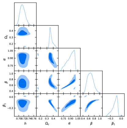
Figure 1: Contour plots for interacting model 1 showing the $1\sigma$ and $2\sigma$ regions. We considered the full joint analysis with Pantheon + BAO + CC + CMB.

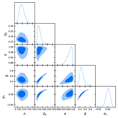
Figure 2: Contour plots for interaction model 2 with the $1\sigma$ and $2\sigma$ regions. We considered the full joint analysis with Pantheon + BAO + CC + CMB.

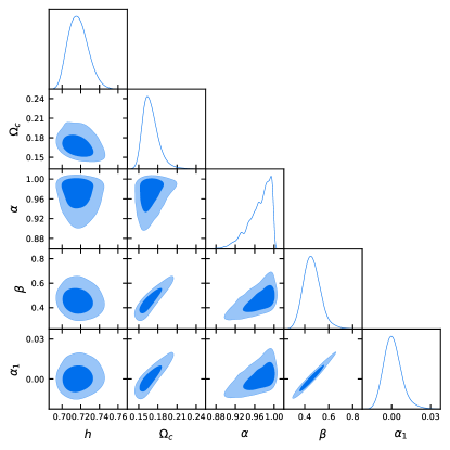
Figure 3: Contour plots for interaction model 3 with the $1\sigma$ and $2\sigma$ regions. We considered the full joint analysis with Pantheon + BAO + CC + CMB.

Table 2: Best fit parameters for the analysis with the Pantheon sample. The last two columns show the logarithm of the Bayes factor ($\ln B$) and the interpretation of the strength of the evidence. Note that $\ln B<-1$ favors the $\Lambda$CDM model.

Model	h	$\Omega_{c}$	$\alpha$	$\beta$	$\alpha_{1}$	$\beta_{1}$	$\ln E$	$\ln B$	Interpretation
$\Lambda$CDM	$0.735\pm 0.015$	$0.257\pm 0.022$	-	-	-	-	$-521.610\pm 0.013$	-	-
HRDE	$0.735\pm 0.015$	$0.182^{+0.072}_{-0.059}$	-	$0.502^{+0.065}_{-0.082}$	-	-	$-523.578\pm 0.019$	$-1.968\pm 0.023$	Weak
MHRDE	$0.735\pm 0.014$	$0.46^{+0.14}_{-0.20}$	$0.754^{+0.24}_{-0.079}$	$0.749^{+0.24}_{-0.090}$	-	-	$-522.490\pm 0.293$	$-0.880\pm 0.293$	Inconclusive
IMHRDE 1	$0.736\pm 0.014$	$0.58^{+0.14}_{-0.26}$	$0.63^{+0.31}_{-0.15}$	$0.813^{+0.18}_{-0.064}$	-	$0.17^{+0.71}_{-0.37}$	$-523.101\pm 0.054$	$-1.491\pm 0.056$	Weak
IMHRDE 2	$0.735\pm 0.014$	$0.58^{+0.23}_{-0.26}$	$0.64^{+0.33}_{-0.16}$	$0.70^{+0.28}_{-0.12}$	$-0.17^{+0.17}_{-0.21}$	-	$-523.635\pm 0.041$	$-2.025\pm 0.043$	Weak
IMHRDE 3	$0.735\pm 0.014$	$0.65^{+0.29}_{-0.17}$	$0.58^{+0.29}_{-0.24}$	$0.72^{+0.26}_{-0.10}$	$-0.17^{+0.16}_{-0.19}$	$-0.17^{+0.16}_{-0.19}$	$-523.883\pm 0.085$	$-2.273\pm 0.086$	Weak
IMHRDE 4	$0.736\pm 0.014$	$0.60^{+0.26}_{-0.23}$	$0.62^{+0.31}_{-0.19}$	$0.72^{+0.25}_{-0.11}$	$-0.20\pm{0.26}$	$0.16^{+0.71}_{-0.41}$	$-523.765\pm 0.068$	$-2.155\pm 0.069$	Weak

Table 3: Best fit parameters for the joint analysis with the dataset Pantheon + BAO + CC + CMB. The last two columns show the logarithm of the Bayes factor ($\ln B$) and the interpretation of the strength of the evidence. Note that $\ln B<-1$ favors the $\Lambda$CDM model.

Model	$h$	$\Omega_{c}$	$\alpha$	$\beta$	$\alpha_{1}$	$\beta_{1}$	$\ln E$	$\ln B$	Interpretation
$\Lambda$CDM	$0.6907\pm 0.0050$	$0.2453\pm 0.0063$	-	-	-	-	$-541.229\pm 0.010$	-	-
HRDE	$0.6951^{+0.0063}_{-0.0076}$	$0.1743\pm 0.0053$	-	$0.488\pm 0.014$	-	-	$-544.438\pm 0.074$	$-3.209\pm 0.075$	Moderate
MHRDE	$0.716^{+0.010}_{-0.012}$	$0.1660\pm 0.0061$	$0.974^{+0.024}_{-0.0088}$	$0.454\pm 0.016$	-	-	$-545.526\pm 0.040$	$-4.297\pm 0.041$	Moderate
IMHRDE 1	$0.7155^{+0.0088}_{-0.012}$	$0.365^{+0.016}_{-0.030}$	$0.895^{+0.10}_{-0.039}$	$0.668^{+0.092}_{-0.12}$	-	$-0.177^{+0.090}_{-0.042}$	$-547.346\pm 0.021$	$-6.117\pm 0.023$	Strong
IMHRDE 2	$0.7182^{+0.0083}_{-0.011}$	$0.1734^{+0.0092}_{-0.0241}$	$0.972^{+0.027}_{-0.0090}$	$0.476^{+0.058}_{-0.096}$	$0.001^{+0.012}_{-0.0099}$	-	$-549.714\pm 0.043$	$-8.485\pm 0.044$	Strong
IMHRDE 3	$0.7173^{+0.0091}_{-0.012}$	$0.1689^{+0.0082}_{-0.014}$	$0.970^{+0.030}_{-0.0099}$	$0.462^{+0.062}_{-0.077}$	$0.0009^{+0.0057}_{-0.0075}$	$0.0009^{+0.0057}_{-0.0075}$	$-550.249\pm 0.066$	$-8.796\pm 0.067$	Strong
IMHRDE 4	$0.7162^{+0.0088}_{-0.011}$	$0.831^{+0.15}_{-0.072}$	$0.49^{+0.11}_{-0.14}$	$0.842^{+0.14}_{-0.063}$	$-0.328^{+0.082}_{-0.12}$	$-0.69^{+0.12}_{-0.16}$	$-549.161\pm 0.043$	$-7.932\pm 0.044$	Strong

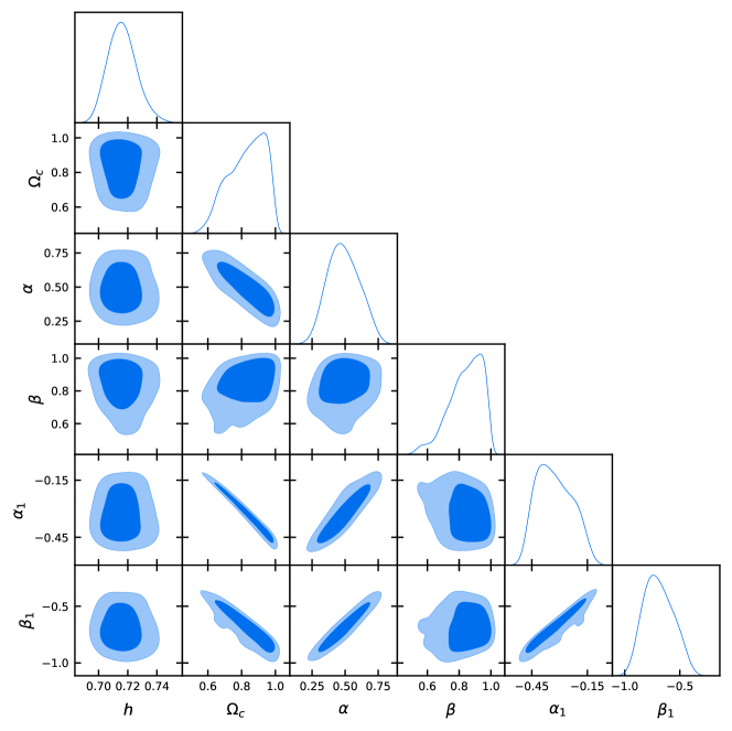
Figure 4: Contour plots for interaction model 4 with the $1\sigma$ and $2\sigma$ regions. We considered the full joint analysis with Pantheon + BAO + CC + CMB.

5 Final Remarks

In this work we have studied interacting modified holographic Ricci dark energy models, where linear interactions are considered. We have found analytical solutions to these scenarios (see Eq. (16)) and we have performed a bayesian model selection analysis. The bayesian comparison is performed with the combination of background data SNe + CC + BAO + CMB (see section 3) and the fiducial model is assumed to be $\Lambda$CDM. Our results indicate that there is strong evidence against the IMHRDE models studied, this conclusion is consistent with several studies where holographic dark energy models have been contrasted with background data Li:2009bn ; delCampo:2011jp ; Wang:2010kwa ; Fu:2011ab ; Feng:2016djj ; George:2019vko ; Akhlaghi:2018knk .

Acknowledgements. AC was partially support by Dirección de Investigación Universidad del Bío-Bío through grant no. GI-172309/C. CRB wants to thank the financial support of Dirección de Postgrado and Dirección de Investigación Universidad del Bío-Bío.

References

- (1) D. H. Weinberg, M. J. Mortonson, D. J. Eisenstein, C. Hirata, A. G. Riess and E. Rozo, Phys. Rept. 530, 87-255 (2013)
- (2) S. Weinberg, Rev. Mod. Phys. 61, 1-23 (1989)
- (3) S. Weinberg, [arXiv:astro-ph/0005265 [astro-ph]].
- (4) L. P. Chimento, A. S. Jakubi, D. Pavon and W. Zimdahl, Phys. Rev. D 67, 083513 (2003)
- (5) Z. K. Guo and Y. Z. Zhang, Phys. Rev. D 71, 023501 (2005)
- (6) D. Pavon and W. Zimdahl, Phys. Lett. B 628, 206-210 (2005) doi:10.1016/j.physletb.2005.08.134 [arXiv:gr-qc/0505020 [gr-qc]].
- (7) L. Verde, T. Treu and A. Riess, “Tensions between the Early and the Late Universe,” [arXiv:1907.10625 [astro-ph.CO]].
- (8) A. G. Riess et al., Astrophys. J. 826, no. 1, 56 (2016)
- (9) A. G. Riess et al., Astrophys. J. 730, 119 (2011) Erratum: [Astrophys. J. 732, 129 (2011)]
- (10) E. J. Copeland, M. Sami and S. Tsujikawa, Int. J. Mod. Phys. D 15, 1753-1936 (2006)
- (11) J. Yoo and Y. Watanabe, Int. J. Mod. Phys. D 21, 1230002 (2012)
- (12) S. Bahamonde, C. G. Böhmer, S. Carloni, E. J. Copeland, W. Fang and N. Tamanini, Phys. Rept. 775-777, 1-122 (2018)
- (13) S. Wang, Y. Wang and M. Li, Phys. Rept. 696, 1-57 (2017)
- (14) A. G. Cohen, D. B. Kaplan and A. E. Nelson, Phys. Rev. Lett. 82, 4971-4974 (1999)
- (15) M. Li, Phys. Lett. B 603, 1 (2004)
- (16) M. Li and Y. Wang, Phys. Lett. B 687, 243-247 (2010)
- (17) S. D. Hsu, Phys. Lett. B 594, 13-16 (2004)
- (18) C. Gao, F. Wu, X. Chen and Y. G. Shen, Phys. Rev. D 79, 043511 (2009)
- (19) R. G. Cai, B. Hu and Y. Zhang, Commun. Theor. Phys. 51, 954-960 (2009) doi:10.1088/0253-6102/51/5/39 [arXiv:0812.4504 [hep-th]].
- (20) L. Xu, W. Li and J. Lu, Mod. Phys. Lett. A 24, 1355-1360 (2009)
- (21) C. J. Feng, Phys. Lett. B 672, 94-97 (2009)
- (22) C. J. Feng, Phys. Lett. B 670, 231-234 (2008)
- (23) M. Li, X. D. Li, S. Wang and X. Zhang, JCAP 06, 036 (2009)
- (24) X. Zhang, Phys. Rev. D 79, 103509 (2009)
- (25) S. Lepe and F. Pena, Eur. Phys. J. C 69, 575-579 (2010)
- (26) K. Y. Kim, H. W. Lee and Y. S. Myung, Gen. Rel. Grav. 43, 1095-1101 (2011)
- (27) S. del Campo, J. Fabris, R. Herrera and W. Zimdahl, Phys. Rev. D 83, 123006 (2011)
- (28) S. del Campo, J. C. Fabris, R. Herrera and W. Zimdahl, Phys. Rev. D 87, no.12, 123002 (2013)
- (29) L. Granda and A. Oliveros, Phys. Lett. B 669, 275-277 (2008)
- (30) L. Granda and A. Oliveros, Phys. Lett. B 671, 199-202 (2009)
- (31) L. Granda and A. Oliveros, [arXiv:0901.0561 [hep-th]].
- (32) L. Granda, W. Cardona and A. Oliveros, [arXiv:0910.0778 [hep-th]].
- (33) Y. Wang and L. Xu, Phys. Rev. D 81, 083523 (2010)
- (34) T. K. Mathew, J. Suresh and D. Divakaran, Int. J. Mod. Phys. D 22, 1350056 (2013)
- (35) B. Hu and Y. Ling, Phys. Rev. D 73, 123510 (2006)
- (36) T. F. Fu, J. F. Zhang, J. Q. Chen and X. Zhang, Eur. Phys. J. C 72, 1932 (2012)
- (37) L. P. Chimento, M. I. Forte and M. G. Richarte, Mod. Phys. Lett. A 28, 1250235 (2013)
- (38) L. P. Chimento and M. G. Richarte, Phys. Rev. D 84, 123507 (2011)
- (39) L. P. Chimento and M. G. Richarte, Phys. Rev. D 85, 127301 (2012)
- (40) L. P. Chimento, M. I. Forte and M. G. Richarte, AIP Conf. Proc. 1471, 39 (2012)
- (41) L. P. Chimento, M. Forte and M. G. Richarte, Eur. Phys. J. C 73, no.1, 2285 (2013)
- (42) P. Pankunni and T. K. Mathew, Int. J. Mod. Phys. D 23, 1450024 (2014)
- (43) F. Arevalo, P. Cifuentes, S. Lepe and F. Peña, Astrophys. Space Sci. 352, 899-907 (2014)
- (44) L. P. Chimento and M. G. Richarte, Eur. Phys. J. C 73, no.4, 2352 (2013)
- (45) A. Oliveros and M. A. Acero, Astrophys. Space Sci. 357, no.1, 12 (2015)
- (46) S. Som and A. Sil, Astrophys. Space Sci. 352, 867-875 (2014)
- (47) N. Mahata and S. Chakraborty, Mod. Phys. Lett. A 30, no.27, 1550134 (2015)
- (48) S. Pan and S. Chakraborty, Int. J. Mod. Phys. D 23, no.11, 1450092 (2014)
- (49) F. Arevalo, P. Cifuentes and F. Pena, Astrophys. Space Sci. 361, no.1, 45 (2016)
- (50) S. Lepe and F. Peña, Eur. Phys. J. C 76, no.9, 507 (2016)
- (51) M. A. Zadeh, A. Sheykhi and H. Moradpour, Int. J. Mod. Phys. D 26, no.08, 1750080 (2017)
- (52) R. Herrera, W. Hipolito-Ricaldi and N. Videla, JCAP 08, 065 (2016)
- (53) L. Feng and X. Zhang, JCAP 08, 072 (2016)
- (54) P. George and T. K. Mathew, [arXiv:1906.08532 [gr-qc]].
- (55) I. Akhlaghi, M. Malekjani, S. Basilakos and H. Haghi, Mon. Not. Roy. Astron. Soc. 477, no.3, 3659-3671 (2018)
- (56) F. Arevalo, A. Cid and J. Moya, Eur. Phys. J. C 77, no.8, 565 (2017)
- (57) B. Santos, N. C. Devi and J. Alcaniz, Phys. Rev. D 95, no.12, 123514 (2017)
- (58) A. Heavens, Y. Fantaye, E. Sellentin, H. Eggers, Z. Hosenie, S. Kroon and A. Mootoovaloo, Phys. Rev. Lett. 119, no.10, 101301 (2017)
- (59) S. Santos da Costa, M. Benetti and J. Alcaniz, JCAP 03, 004 (2018)
- (60) U. Andrade, C. Bengaly, J. Alcaniz and B. Santos, Phys. Rev. D 97, no.8, 083518 (2018)
- (61) T. Ferreira, C. Pigozzo, S. Carneiro and J. Alcaniz, [arXiv:1712.05428 [astro-ph.CO]].
- (62) A. Cid, B. Santos, C. Pigozzo, T. Ferreira and J. Alcaniz, JCAP 03, 030 (2019)
- (63) M. Moresco et al., JCAP 1605, no. 05, 014 (2016)
- (64) D. M. Scolnic et al., Astrophys. J. 859, no. 2, 101 (2018)
- (65) F. Beutler et al., Mon. Not. Roy. Astron. Soc. 416, 3017 (2011)
- (66) A. J. Ross, L. Samushia, C. Howlett, W. J. Percival, A. Burden and M. Manera, Mon. Not. Roy. Astron. Soc. 449, no. 1, 835 (2015)
- (67) M. Ata et al., Mon. Not. Roy. Astron. Soc. 473, no. 4, 4773 (2018)
- (68) J. Hou et al., Mon. Not. Roy. Astron. Soc. 480, no. 2, 2521 (2018)
- (69) S. Alam et al. [BOSS Collaboration], Mon. Not. Roy. Astron. Soc. 470, no. 3, 2617 (2017)
- (70) H. du Mas des Bourboux et al., Astron. Astrophys. 608, A130 (2017)
- (71) P. A. R. Ade et al. [Planck Collaboration], Astron. Astrophys. 594, A14 (2016)
- (72) R. Jimenez and A. Loeb, Astrophys. J. 573, 37 (2002)
- (73) L. Verde, P. Protopapas and R. Jimenez, Phys. Dark Univ. 5-6, 307 (2014)
- (74) D. J. Eisenstein et al. [SDSS Collaboration], Astrophys. J. 633, 560 (2005)
- (75) D. J. Eisenstein and W. Hu, Astrophys. J. 496, 605 (1998)
- (76) J. Evslin, A. A. Sen and Ruchika, Phys. Rev. D 97, no. 10, 103511 (2018)
- (77) N. Aghanim et al. [Planck Collaboration], arXiv:1807.06209 [astro-ph.CO].
- (78) R. Trotta, Contemp. Phys. 49, 71 (2008)
- (79) F. Feroz and M. Hobson, Mon. Not. Roy. Astron. Soc. 384, 449 (2008)
- (80) F. Feroz, M. Hobson and M. Bridges, Mon. Not. Roy. Astron. Soc. 398, 1601-1614 (2009)
- (81) A. G. Riess et al., Astrophys. J. 861, no. 2, 126 (2018)
- (82) E. Komatsu et al. [WMAP Collaboration], Astrophys. J. Suppl. 192, 18 (2011)
- (83) G. Mangano, G. Miele, S. Pastor, T. Pinto, O. Pisanti and P. D. Serpico, Nucl. Phys. B 729, 221 (2005)