Benchmarking neural embeddings for link prediction in knowledge graphs under semantic and structural changes

Abstract

Recently, link prediction algorithms based on neural embeddings have gained tremendous popularity in the Semantic Web community, and are extensively used for knowledge graph completion. While algorithmic advances have strongly focused on efficient ways of learning embeddings, fewer attention has been drawn to the different ways their performance and robustness can be evaluated. In this work we propose an open-source evaluation pipeline, which benchmarks the accuracy of neural embeddings in situations where knowledge graphs may experience semantic and structural changes. We define relation-centric connectivity measures that allow us to connect the link prediction capacity to the structure of the knowledge graph. Such an evaluation pipeline is especially important to simulate the accuracy of embeddings for knowledge graphs that are expected to be frequently updated.

url]Code is available open source https://github.com/plumdeq/neuro-kglink

1 Introduction

Link prediction, in general, is a problem of finding the missing or unknown links among inter-connected entities. This assumes that entities and links can be represented as a graph, where entities are nodes and links (symmetric relationships) are edges (arcs if relationships are asymmetric). This prediction problem has been most probably defined for the first time in the social network analysis community [1], however, it has soon become an important problem in other domains, and in particular in large-scale knowledge-bases [2], where it is used to add missing data and discover new facts. When we are dealing with the link prediction problem for knowledge-bases, the semantic information contained within is usually encoded as a knowledge graph (KG) [3]. For the purpose of this manuscript, we treat a knowledge graph as a graph where links may have different types, and we conform to the closed-world assumption. This means that all the existing (asserted) links are considered positive, and all the links which are unknown, and obtained via knowledge graph completion, are considered negative (Figure 1).

Figure 1: A sample KG with three entities and two relation types. Positive links are drawn in bold, negative in dotted edge styles.

This separation into positive and negative links (examples) naturally allows us to treat the link prediction problem as a supervized classification problem with binary predictors. However, while this separation enables a wealthy body of available and well-studied machine learning algorithms to be used for link prediction, the main challenge is how to find the best representations for links. And this is the core subject of the recent research trend in learning suitable representations for knowledge graphs, largely dominated by the so-called neural embeddings (initially introduced for language modelling [4]). Neural embeddings are numeric representations of nodes, and/or relations of the knowledge graph, in some continuous and dense vector space. These embeddings are learned with neural networks by optimizing a specific objective function. Usually, the objective function models the constraints that neighboring nodes are embedded close to each other, and the nodes that are not directly connected, or separated via long paths in the graph, are embedded to stay far apart. A link in a knowledge graph is then represented as a combination of node and/or relation type embeddings [2, 5].

1.1 Benchmarking accuracy and robustness of neural embeddings

There are two major ways of measuring the accuracy of embeddings of entities in a knowledge graph for link prediction tasks, inspired by two different fields: information retrieval [6, 7, 8, 2, 9, 10, 11] and graph-based data mining [12, 13, 14, 15, 16, 17]. Information retrieval inspired approaches seem to favor node-centric evaluations, which measure how well the embeddings are able to reconstruct the immediate neighbourhood for each node in the graph; these evaluations are based on the mean rank measurement and its variants (mean average precision, top $k$ results, mean reciprocal rank). And graph-based data mining approaches tend to measure link-equality by recurring to the evaluation measurements such as, ROC AUC and F-measure. See [18] for more discussion on node- and link-equality measures.

Besides evaluating the accuracy, some works have focused their attention on issues that might hinder the appropriate evaluation of embeddings. For instance, there is the issue of imbalanced classes – many more negatives than positives – when the link prediction in graphs is treated as a classification problem [14]. In the bioinformatics community the problem of imbalanced classes can be circumvented by considering negative links that have a biological meaning, truncating thus many potential negative links that are highly improbable biologically [16]. Other works have demonstrated that if no care is applied while splitting the datasets, we might end up producing biased train and test examples, such that the implicit information from the test set may leak into the train set [19, 20]. Kadlec et al. [9] have mentioned that the fair optimization of hyperparameters for competing approaches should be considered, as some of the reported KG completion results are significantly lower than what they potentially could be. In the life sciences domain, the time-sliced graphs as generators for train and test examples have been proposed as a more realistic evaluation benchmark [18], as opposed to the randomly generated slices of graphs.

In addition to reference implementations accompanying scientific papers that propose novel embedding methodologies, there is a wealthy core of open-source initiatives that provide a one stop solution for efficient training of knowledge graph embeddings. For instance, pkg2vec [21] and PyKeen [22] implement many of the state-of-the-art KG embedding techniques, with the focus on reproducibility and efficiency. While the community has many options for the efficient KG embedding implementations, we believe that fewer attention has been drawn to evaluating neural embeddings when knowledge graphs may exhibit structural changes. In this work we aim to make this gap narrower. Our work is closest in spirit to Goyal et al. [23] – an evaluation benchmark for graph embeddings that tries to explain which intrinsic properties of graphs make certain embedding models perform better. Unlike us, the authors consider knowledge graphs with only one type of relation.

The rest of this manuscript is organized as follows: in the Methods section (Section 2) we define the notation, present knowledge graphs we used to evaluate our approach, and formalize the evaluation pipeline. Then, in the Section 3 we introduce connectivity descriptors that allow us to capture the structural change in knowledge graphs. Sections 4, 5 report our experiments and analysis. Finally, we conclude our manuscript in the Section 6.

1.2 Contributions of this work

In our work we define semantic similarity descriptors for knowledge graphs, and correlate the performance of neural embeddings to these descriptors. The big take away from this work is that it is possible to improve the accuracy of the embeddings by adding more instances of semantically related relations. For instance, we can improve overall accuracy of knowledge graph embeddings by increasing the number of semantically related relations. This means that if we have access to information that is partially redundant (triples for an inferred relation, or a semantically related relation) this may improve overall accuracy. Moreover, by using our benchmark, we can perform a more fine-tuned error analysis, by examining which specific type of links pose the most problem for overall link prediction. Finally, by examining the correlation of accuracy scores to the semantic similarity descriptors we can explain the performance of neural embeddings, and predict their performance by simulating modifications to the knowledge graphs.

2 Methods

2.1 Notation and terminology

Throughout this manuscript we employ the triple-oriented treatment of knowledge graphs. As such, a knowledge graph $KG$ is simply a set of triples $(e_{i},r_{i},e_{j})\in KG$, where $e_{i},e_{j}\in\textsc{entities}(KG)$ are some entities, and $r_{i}\in\textsc{relations}(KG)$ are its relation types, or simply relations. We assume that entities and relation types are disjoint sets, i.e., $\textsc{entities}(KG)\neq\textsc{relations}(KG)$. Let $Pos_{KG}$ denote all the existing triples in the $KG$, i.e., triples $(e_{i},r_{i},e_{j})\in KG$, and let $Neg_{KG}$ denote the non-existing triples $(\bar{e_{i}},\bar{r_{i}},\bar{e_{j}})\not\in KG$ via the knowledge graph completion ($\bar{e_{i}},\bar{e_{j}}\in\textsc{entities}(KG)$, $\bar{r_{i}}\in\textsc{relations}(KG)$). Similarly, $Pos_{r_{i}}$ and $Neg_{r_{i}}$ denote the existing and non-existing triples involving a relation $r_{i}$, respectively. Obviously, in every triple of $Pos_{r_{i}}$ or $Neg_{r_{i}}$ the relation type is fixed to $r_{i}$. For each relation type $r_{i}$, $\textsc{domain}(r_{i}),\textsc{range}(r_{i})\in\textsc{entities}(KG)$ indicate the entities that belong to the domain and range of a relation $r_{i}$. To describe the process of sampling some triples, we use the notation $\alpha X,\alpha\in[0,1]$, where $X$ is any set of triples. For instance, $(\alpha=0.8)Pos_{r_{i}}$ is a sampled set of triples involving $r_{i}$, and consisting of $80\%$ of triples from $Pos_{r_{i}}$. Occasionally, when we write $(e_{i},\_,e_{j})$ we refer to a set of triples where $e_{i},e_{j}$ are fixed, and the relation type $\_\in\textsc{relations}(KG)$ is free.

2.2 Knowledge graphs

We run our experiments on four different knowledge graphs: WN11 [19] (subset of original WordNet dataset [24] brought down to 11 types of relations, and without inverse relation assertions), FB15k-237 [19] (a subset of Freebase knowledge graph [25] where inverse relations have been removed), UMLS (subset of the Unified Medical Language System [26] semantic network) and BIO-KG (comprehensive biological knowledge graph [16]). WN11, FB15k-237 and UMLS have been downloaded (December 2017) from the ConvE [20] GitHub repository, and BIO-KG has been downloaded (September 2017) from the official link indicated in the supplementary material for [16]. Details on the derivation of subsets for Wordnet and Freebase knowledge graphs can be found in [19, 20].

2.3 Training and evaluating neural embeddings

Figure 2: Overview of the pipeline for training specialized and generalized neural embeddings for link prediction.

Our work builds upon the earlier proposed framework [16] to both learn and evaluate neural embeddings for the knowledge graphs, which we extend to make it more scalable. Throughout this manuscript we refer to the original framework as specialized embeddings approach. In a nutshell this approach learns and evaluates specialized embeddings for each relation type $r_{i}$ of entities of $KG$ as follows: a) we generate the retained graph where we delete some of the triples involving $r_{i}$, then b) we compute the embeddings of the entities on this resulting retained graph, finally, c) we assess the quality of these specialized embeddings on relation $r_{i}$ by training and testing binary predictors on positive and negative triples involving $r_{i}$. These three steps are detailed in Figure 2 in the specialized embeddings box. The arrows labelled with “a” in Figure 2 symbolize the generation of retained graphs for relations $r_{1}$ and $r_{2}$, those marked with “b” computation of the entity embeddings, and “c” represents the training and testing binary classifiers for each relation type.

The inconvenience of the specialized embeddings approach is that we need to compute entity embeddings for each relation type separately, which is a serious scalability issue when the number of relation types in the knowledge graph becomes big. To circumvent this issue, we propose to train generalized neural embeddings for all relation types once, as opposed to training specialized embeddings for a specific relation $r_{i}$ (Figure 2, generalized embeddings box). Specifically, we generate only one retained graph, where we delete a fraction of triples for each relation type $r_{i}$ (arrow marked with “a” on the bottom of Figure 2). This retained graph is then used as a corpus for the computation of entity embeddings (“b”), which are then assessed with binary predictors for each relation type $r_{i}$ as in the specialized case (arrows marked with “c” on the bottom of Figure 2). Evidently, this approach is more scalable and economic, since we only compute and keep one set of entity embeddings per knowledge graph.

In what follows we formalize the pipeline for link prediction with specialized and generalized neural embeddings, and we give a thorough description of steps “a”, “b” and “c” (Figure 2).

2.3.1 Generation of retained graphs (step a)

By treating the problem of evaluation of the quality of the embeddings in a set-theoretic approach, we can define the following datasets:

1. $Pos_{KG}-(1-\alpha)Pos_{r_{i}}$ a specialized retained graph on $r_{i}$ – training corpus for unsupervised learning of local to $r_{i}$ entity embeddings $\gamma_{r_{i}}(e_{i})$ (in Figure 3 this set is demarcated with bold contour in the upper left corner),

2. $Pos_{KG}-\bigcup_{r_{i}}(1-\alpha)Pos_{r_{i}}$ a generalized retained graph on all relations $r_{i}$ – training corpus for unsupervised learning of global entity embeddings $\gamma(e_{i})$,

3. $\forall r_{i},\alpha Pos_{r_{i}}\bigcup\alpha Neg_{r_{i}}$ – train examples for the binary classifier for $r_{i}$,

4. $\forall r_{i},(1-\alpha)Pos_{r_{i}}\bigcup(1-\alpha)Neg_{r_{i}}$ – test examples for the binary classifier for $r_{i}$.

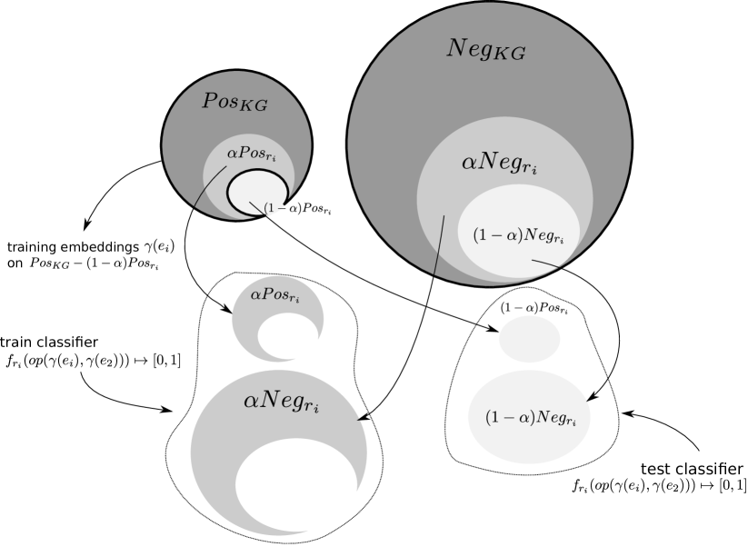
Figure 3: Schematic representation of the pipeline for the evaluation of the embeddings. $Neg_{KG}$ and its derivations (e.g., $\alpha Neg_{r_{i}}$) appear bigger visually to indicate that the elements are sampled from a much bigger set of all possible negative links.

2.3.2 Neural embedding model (step b)

In this work we employ a shallow unsupervised neural embedding model [17], which aims at learning entity embeddings in a dense $d$-dimensional vector space. The model is simple and fast, and it embeds the entities that appear in the positive triples close to each other, and places the entities that appear in negative triples farther appart. As in many neural embedding approaches, the weight matrix of the hidden layer of the neural network serves the role of the look-up matrix (the matrix of embeddings - latent vectors). The neural network is trained by minimizing, for each positive triple $x_{i}=(e_{i},\_,e_{j})$ in the specialized ($x_{i}\in Pos_{KG}-(1-\alpha)Pos_{r_{i}}$), or generalized graphs ($x_{i}\in Pos_{KG}-\bigcup_{r_{i}}(1-\alpha)Pos_{r_{i}}$), the following loss function

$$\sum_{(e_{i},\_,\bar{e_{j}})\in Neg_{KG}}L\left(\text{sim}(e_{i},e_{j}),\text{sim}(e_{i},\bar{e_{1}}),\ldots,\text{sim}(e_{i},\bar{e_{k}})\right).$$

Where, for each positive triple $x_{i}$, we embed entities $e_{i},e_{j}$ close to each other, such that $e_{i}$ stays as far as possible from the $k$ negative entities $\bar{e_{1}},\ldots,\bar{e_{k}}$. The similarity function sim is task-dependent and should operate on $d$-dimensional vector representations of the entities (e.g., standard Euclidean dot product). The loss function $L$ is a softmax, that compares the positive example ($e_{i},e_{j}$) to all the negative examples (($e_{i},x),x\in Neg_{KG}$).

2.3.3 Link prediction evaluation with binary classifiers (step c)

To quantify confidence in the trained embeddings, we perform the repeated random sub-sampling validation for each classifier $f_{r_{i}}$. That is, for each relation $r_{i}$ we generate $k$ times: retained graph $Pos_{KG}-(1-\alpha)Pos_{r_{i}}$ corpus for unsupervised learning of entity embeddings $\gamma_{r_{i}}(e_{i})$) and train $\alpha Pos_{r_{i}}\bigcup\alpha Neg_{r_{i}}$ and test $(1-\alpha)Pos_{r_{i}}\bigcup(1-\alpha)Neg_{r_{i}}$ splits of positive and negative examples. Link prediction is then treated as a binary classification task with a classifier $f_{r_{i}}:op(\gamma(e_{i}),\gamma(e_{j})))\mapsto[0,1]$, where $op$ is a binary operator that combines entity embeddings $\gamma(e_{i}),\gamma(e_{j})$ into one single representation of the link $(e_{i},r_{i},e_{j})$. The performance of the classifier is measured with the standard performance measurements (e.g., F-measure, ROC AUC).

2.4 Evaluation benchmark summary and implementation

The whole evaluation pipeline is summarized in Algorithm 1. In our experiments the specialized and generalized neural embeddings are trained with the StarSpace toolkit [10] in the train mode 1 (see StarSpace specification) with fixed hyperparameters: embedding size $d=50$, number of epochs 10, all other parameters set to default. Classification results are obtained with the scikit Python library [27], statistical analysis is performed with Pandas [28]. Our experiments were performed on a high performance cluster, with modern PCs controlling multiple NVIDIA GPUs (GTX1080 and GTX1080TI). To demonstrate the high-flexibility of our pipeline, we also consider knowledge graph embeddings provided with the state-of-the-art DistMult [7] and ComplEx [8] models. Both of these models for our experiments were implemented in PyTorch (v1.2).

Algorithm 1 Evaluation of specialized and generalized knowledge graph embeddings

1$KG,\alpha,J$

2for each sub-sample validation run

3for $j\in 1,\ldots,J$ do

4   generate retained graph on all $r_{i}$,

5   and compute generalized embeddings

6    $X$ $\leftarrow$ $Pos_{KG}-\bigcup_{r_{i}}(1-\alpha)Pos_{r_{i}}$

7    $\gamma(e_{i})$ $\leftarrow$ Embeddings($X$)

8

9    for $r_{i}\in\textsc{relations}(KG)$ do

10        generate retained graph on $r_{i}$,

11        and compute specialized embeddings

12         $X_{r_{i}}$ $\leftarrow$ $Pos_{KG}-(1-\alpha)Pos_{r_{i}}$

13         $\gamma_{r_{i}}(e_{i})$ $\leftarrow$ Embeddings($X_{r_{i}}$)

14

15        generation of train/test examples for $r_{i}$

16         $train_{r_{i}}$ $\leftarrow$ $\alpha Pos_{r_{i}}\bigcup\alpha Neg_{r_{i}}$

17         $test_{r_{i}}$ $\leftarrow$ $(1-\alpha)Pos_{r_{i}}\bigcup(1-\alpha)Neg_{r_{i}}$

18        evaluate quality of specialized embeddings

19         $F1^{j}_{r_{i}}$ $\leftarrow$ $f_{r_{i}}(train_{r_{i}},test_{r_{i}},\gamma_{r_{i}}(e_{i}))$

20    end for

21        evaluate quality of generalized embeddings

22    $F1^{j}$ $\leftarrow$ $f_{r_{i}}(train_{r_{i}},test_{r_{i}},\gamma(e_{i}))$

23end for

24

25average specialized embeddings evaluations

26for $r_{i}\in\textsc{relations}(KG)$ do

27    $\widetilde{F1}_{r_{i}}$ $\leftarrow$ $\sum_{j}F1^{j}_{r_{i}}$

28end for

29

30average generalized embeddings evaluations

31$\widetilde{F1}$ $\leftarrow$ $\sum_{j}F1^{j}$

3 Structure of knowledge graphs and their change

In this section we introduce a few descriptors that are necessary to capture the variability and change in the structure of knowledge graphs. In addition to standard descriptors that describe the structure of knowledge graphs syntactically (number of entities, relations and triples), we define descriptors that measure the positive to negative ratio for each relation, and the semantic similarity of relations in the knowledge graph. These descriptors will be then used to evaluate and explain the performance of neural embeddings.

The variation of syntactic structure of the four graphs is summarized in Table 1 under the label Global. By analyzing these global descriptors, $|\textsc{entities}|$, $|\textsc{relations}|$, $|Pos_{KG}|$, we see that we have one small knowledge graph (UMLS), two medium-sized graphs (WN11, FB15K-237) and one very large biological graph (BIO-KG). In what follows we define the descriptors that are used in the rest of the Table 1.

	Semantic		Pos/Neg ratio		Global
$G$	$\lVert S\rVert_{F}$	$\lVert S^{\prime}\rVert_{F}$	mean($\mu_{r_{i}}$) %	mean($z_{r_{i}}$) %	$|\textsc{entities}|$	$|\textsc{relations}|$	$|Pos_{KG}|$
WN11	0.81	<0.01	0.68	5e-4	40,943	11	93,003
FB15k-237	19.09	3.84	17.33	6e-4	14,541	237	310,116
BIO-KG	1.31	0	0.73	1e-4	346,225	9	1,619,239
UMLS	9.46	2.31	60	7e-1	137	46	6,527

Table 1: Statistics of descriptors that measure the variability in the structure of the four considered knowledge graphs. Global descriptors describe knowledge graphs syntactically in terms of number of entities, relations and triples. Descriptors that measure the positive to negative ratio (Pos/Neg ratio, see Equations 1, 2) are averaged for all relations, and show the percentage of positive to (semantic) negative examples. Finally, the semantic similarity of relations in the knowledge graphs (Semantic) is summarized with the Frobenius norm on the Jaccard similarity matrices (Equations 3, 4).

3.1 Positive to negative ratio descriptors

To measure the ratio of positive to negative examples in a knowledge graph, for a fixed relation $r_{i}$, we use the descriptors $\mu_{r_{i}}$ and $z_{r_{i}}$, defined as follows:

$$\mu_{r_{i}} =\frac{|Pos_{r_{i}}|}{|\textsc{domain}(r_{i})|\times|\textsc{range}(r_{i})|},$$ (1)

$$z_{r_{i}} =\frac{|Pos_{r_{i}}|}{|\textsc{entities}|\times(|\textsc{entities}|-1)}.$$ (2)

For an induced graph $G_{r_{i}}$ – consisting of all the triples involving relation $r_{i}$ of a knowledge graph – both descriptors measure how close is $G_{r_{i}}$ to being complete (fully connected). Intuitively, if a graph is only half complete (Figure 4, left), then we could potentially generate as many negatives as positives. However, if the graph is complete (all entities are connected, Figure 4, right), then there will be no negative links generated. In $\mu_{r_{i}}$ we restrict the space of negative examples by generating semantically plausible links, i.e., we only consider unconnected pairs from the domain and range of $r_{i}$. Analogously, $z_{r_{i}}$ relaxes this restrictions, i.e., the negatives can be generated from all possible pairs of entities in the knowledge graph. We hypothesize that the performance of a binary link predictor of type $r_{i}$ should be positively correlated with both $\mu_{r_{i}}$ and $z_{r_{i}}$, i.e., the more training examples of type $r_{i}$ there are (the more connected $G_{r_{i}}$ is) the better is the performance of the binary predictor for $r_{i}$.

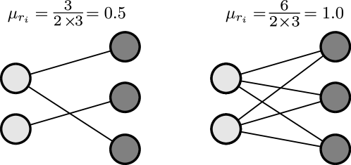
Figure 4: $\mu_{r_{i}}$ - ratio of positive to negative examples for the relation $r_{i}$. Effectively, it is maximized when the induced graph $G_{r_{i}}$ is closer to being complete (all entities are interconnected). Lighter nodes indicate domain and darker nodes indicate range of $r_{i}$.

Focusing on the positive to negative ratio descriptors, under the label Pos/Neg ratio in Table 1, we see that we have two dense graphs (UMLS and FB15k-237), and two very sparse graphs (WN11 and BIO-KG). When we restrict the negative sample generation to only plausible semantic examples ($\mu_{r_{i}}$), UMLS has on average 60% positive triples per relation, and FB15k-237 17.33%. On the other hand, the two sparse graphs, BIO-KG, and WN11, both have less than 1% positive triples. This suggests that for these sparse graphs, the binary prediction for any relation is extremely imbalanced, which may potentially hinder the performance of neural embedding models. If we consider negative sample generation without any semantic restriction ($z_{r_{i}}$), then all binary tasks are highly imbalanced.

3.2 Descriptors to measure semantic similarity of relations

We introduce two descriptors that capture the amount to which the relations in the knowledge graph are similar one to another. $S_{r_{1},r_{2}}$ measures the number of shared instances between the relations, and $S^{\prime}_{r_{1},r_{2}}$ measures the proportion of shared entities either in the domain or range of the two relations. Both are based on the Jaccard similarity index, where sets are defined as in Equations 3, 4. Notice that $S_{r_{1},r_{2}}$ can be seen as the degree of the role equivalence in the description logic sense; the higher it is the more two relations are semantically similar (contain the same pairs of entities). And the $S^{\prime}_{r_{1},r_{2}}$ is higher when the two relations interconnect the same entities. Note that in $S$ elements of sets are tuples $(e_{i},e_{j})$, and in $S^{\prime}$ elements are entities $e_{i}$.

$$S_{r_{1},r_{2}} =\frac{|Pos_{r_{1}}\bigcap Pos_{r_{2}}|}{|Pos_{r_{1}}\bigcup Pos_{r_{2}}|}$$ (3)

$$S^{\prime}_{r_{1},r_{2}} =\frac{|X(r_{1})\bigcap X(r_{2})|}{|X(r_{1})\bigcup X(r_{2})|},X(r_{i})=\textsc{domain}(r_{i})\cup\textsc{range}(r_{i})$$ (4)

When we consider semantic similarity among the relations in our four knowledge graphs, we see the similar pattern as for the descriptors that measure positive to negative ratio. In Figure 5 we demonstrate heatmaps of semantic similarity of relations for four graphs.

Figure 5: Heatmaps of semantic similarity among the relations in the four considered knowledge graphs. All matrices are symmetric and square, and have the size $|\textsc{relations}|\times|\textsc{relations}|$. $S_{ij}$ measures the semantic similarity as the Jaccard index on the shared instances (pairs of entities), and $S^{\prime}_{ij}$ measures the semantic similarity as the Jaccard index on the shared entities, in the domain or range of the two relations.

We can observe that UMLS and FB15k-237 have many similar relations ($S_{r_{1},r_{2}}\to 1$), very few of WN11 relations share instances, and the relations of BIO-KG do not share any instances at all ($\forall_{r_{1},r_{2}}S_{r_{1},r_{2}}=0$). If we consider the semantic similarity in terms of shared entities, we see that, although BIO-KG and WN11 have dissimilar relations ($S_{r_{1},r_{2}}\to 0$), they still can share information for the shared embeddings ($S^{\prime}_{r_{1},r_{2}}>0$). To see it consider two relations $r_{1},r_{2}$ that do not share instances ($S_{r_{1},r_{2}}\to 0$), but do share entities $e_{1},\ldots,e_{n}$ that they interconnect ($S^{\prime}_{r_{1},r_{2}}>0$). In this situation, the training examples for $r_{1}$ and $r_{2}$ may share information during the learning phase and improve the quality of embeddings for $e_{1},\ldots,e_{n}$. Using these two similarity matrices, we can define measures of semantic similarity among relations in the whole knowledge graph by taking the Frobenius norm ($\lVert S\rVert_{F}:=\sqrt{\sum_{ij}|S_{ij}|^{2}}$) of matrices $S$ and $S^{\prime}$ (Table 1, label Semantic).

Overall, the proposed connectivity descriptors capture well the semantic and structural variability of knowledge graphs, and will allow us to make more nuanced evaluation of neural embeddings.

4 Benchmarking specialized and generalized embeddings under structural change

The goal of our experiments is to empirically investigate if, and when, the generalized neural embeddings attain similar performance as the specialized embeddings, for the four considered datasets. To do so, we first generate the retained graphs, and the train and test datasets. The retained graphs are generated for each relation type $r_{i}$ in the case of specialized embeddings, and only once for the generalized embeddings. We always keep the 1:1 ratio for the positive and negative examples. When we sample the negatives for a relation $r_{i}$, we only consider the triples $(\bar{e_{i}},r_{i},\bar{e_{j}})$ where the entities come from the domain ($\bar{e_{i}}\in\textsc{domain}(r_{i})$) and the range ($\bar{e_{i}}\in\textsc{range}(r_{i})$) of $r_{i}$. Embeddings are computed from retained graphs, and then evaluated on train and test datasets. Note that we only provide results for generalized embeddings for FB15k-237, since the computation of specialized embeddings for 237 relations of FB15k-237 would take months (on our machine) to finish. The evaluation of embeddings for one relation type $r_{i}$ is performed with the logistic regression classifier $f_{r_{i}}(op(\gamma(e_{i}),\gamma(e_{j})))$, where $op$ is the vector concatenation operator. To test the robustness of embeddings we perform evaluations with limited information, i.e., the size of the retained graphs controlled by $\alpha\in\{0.2,0.5,0.8\}$, and we analyze the amount of missed embeddings in all experiments. All of our results are presented as averages of 10 repeated random sub-sampling validations. We thus report mean F-measure scores and their standard deviations.

4.1 Comparing accuracy

In Figure 6 we present distributions of averaged F1 scores, which measure the accuracy of embeddings, and ratios ($[0,1])$ of missed examples at training and testing of the binary classifiers $f_{r_{i}}$. As such, the overall performance of specialized or generalized embeddings on one knowledge graph is characterized by these three distributions over all relations in the given knowledge graph. The performance of embeddings is compared with varying amount of information present at the time of training of neural embeddings (parameter $\alpha$). All distributions in Figure 6 are estimated and normalized with kernel density interpolation from actual histograms.

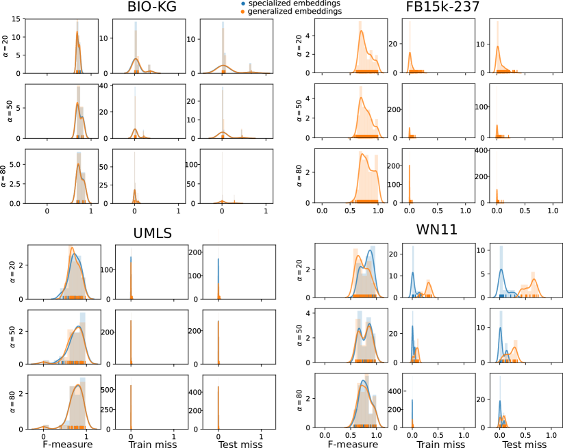
Figure 6: Distributions of F1 scores, ratio of missing entities at trainging, and at testing, for specialized and generalized embeddings, for four graphs.

In the three knowledge graphs: BIO-KG, UMLS and WN11, distributions converge as we increase the amount of available information (e.g., $\alpha\to 1$), which supports of the hypothesis of this manuscript, that the generalized embeddings may yield the similar (if not the same) performance as specialized embeddings. When we consider BIO-KG, the F1 and missing examples distributions for specialized and generalized neural embeddings converge almost to identical distributions, even when the overall amount of information is low (e.g., only 20 % of available triples). This may be explained by a relatively big size of available positive examples per relation type $|Pos_{r_{i}}|$ (hundreds of thousands of available triples per relation). Though, $\text{mean}(z_{r_{i}})$ and $\text{mean}(\mu_{r_{i}})$ (Table 1) are very similar for BIO-KG and WN11, differences between specialized and generalized embeddings for WN11 are much more characterized, than in the case of BIO-KG. In particular, neural embeddings for WN11 are very sensitive to $\alpha$, the less information there is the more is the intra-discrepancy in specialized and generalized distributions for the same scores (F1 and the ratio of missed examples). The amount of missed examples is very high for both specialized and generalized cases, for smaller values of $\alpha<0.8$, and distributions converge when $\alpha=0.8$. The most regular behavior is demonstrated by neural embeddings trained on UMLS corpora, where missing examples rates are all almost zero, even when $\alpha=0.2$. Shapes of the F1 distributions are very similar for all values of $\alpha$, intra-discrepancies are very low. These observations allow us to hypothesize that similar trends might exist for the FB15k-237 knowledge graph, since UMLS and FB15k-237 have similar distributions of $\mu_{r_{i}}$ and $z_{r_{i}}$.

To summarize, as we increase the amount of available information during the computation of neural embeddings ($\alpha\to 1$) intra-discrepancies between specialized and the generalized embeddings become negligible. And this is good news, since training generalized embeddings is $|\textsc{relations}(KG)|$-times faster than training specialized embeddings for each relation $r_{i}$, with the strong evidence that if we have enough information we can achieve the same performance.

4.2 Comparing average performance

We recall that each distribution’s sampled point is obtained by averaging results of $k$ repeated experiments for one relation $r_{i}$. To directly compare distributions, we compare their means and standard deviations, and, as such, we are comparing the average performance of $|\textsc{relations}(KG)|$ binary classifiers for specialized and generalized neural embeddings, with the varying parameter $\alpha$. Figure 7 depicts the average performance of all binary classifiers and its standard deviation for the four knowledge graphs.

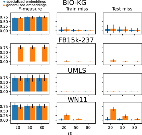
Figure 7: Averaged F1 scores, ratio of missing entities at trainging, and at testing, for specialized and generalized embeddings, for four graphs.

As expected, the performance of specialized embeddings is better than the performance of generalized embeddings, however differences are very slim. BIO-KG and UMLS demonstrate that, as we increase $\alpha$, the average F1 score increases in both cases, however, so does the standard deviation as well. WN11, on the other hand, demonstrates a counter-intuitive trend where the best performance of specialized embeddings occurs when less information is available. And, for specialized embeddings, the F1 score decreases slightly when we include more information during the computation of neural embeddings. This maybe explained by an increased amount of missing examples, both during training and testing of the binary classifier. Due to a very sparse connectivity of the induced graphs $G_{r_{i}}$ of WN11, when we only consider $20\%$ of available triples – we exclude 80 % of available links – many entities are likely to become disconnected. This means that no embeddings are learned for them, and, as a result, the binary classifier is both trained and tested on fewer examples.

5 DistMult vs. ComplEx

In this experiment, our goal is to compare two of the most popular knowledge graph embedding models, DistMult [7] and ComplEx [8], by using our relation-centric ablation benchmark. In particular, our mission is to explain which intrinsic properties of graphs directly impact the accuracy of neural models. In contrast to our previous experiment, we perform random ablations on each relation type $\alpha_{r}\sim N(0,1),\forall r\in\textsc{relations}(KG)$. For each knowledge graph we train 10 DistMult and 10 ComplEx models. We fix the embedding dimension to 200, and we use Adam optimizer. Each time models are trained for 50 epochs. The accuracy is assessed with mean rank and mean reciprocal rank metrics. In Table 2 we report mean (with standard deviation) MR and MRR performance of two models on four datasets, as well as averaged performance of models for all graphs. Overall, ComplEx is slightly better than DistMult ($0.76(0.2)$ vs. $0.75(0.26)$, mean(SD)) however their performances stay within the confidence intervals for all graphs. If we look at the performance of models for specific graphs, the differences are more apparent. In Figure 8 we present point estimates and confidence intervals of the MRR metric for a specific graph, with horizontal lines accentuating the difference in accuracy for the two models. ComplEx is better at UMLS and WN11. DistMult on the other two.

		MRR (mean (SD))	MR (mean (SD))
model	$G$
ComplEx	BIO-KG	0.67 (0.06)	30,810.75 (6330.92)
	FB15k-237	0.92 (0.02)	63.56 (20.61)
	WN11	0.5 (0.15)	6,033.56 (2360.53)
	UMLS	0.89 (0.02)	2.87 (0.36)
		0.76 (0.2)	6144.39 (10,846.1)
DistMult	BIO-KG	0.92 (0.04)	189.26 (42.09)
	FB15k-237	0.95 (0.01)	67.96 (14.48)
	WN11	0.38 (0.21)	8,347.39 (4016.02)
	UMLS	0.83 (0.03)	4.27 (0.78)
		0.75 (0.26)	2,432.64 (4321.82)

Table 2: Average performance of DistMult and ComplEx on four knowledge graphs. MRR and MR are reported as means of 10 runs (standard deviation in parenthesis). Additionally, we report average performance per model for all knowledge graphs (with standard deviation).

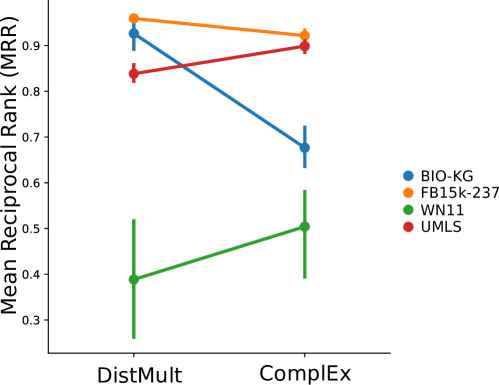
Figure 8: Point estimate of performances for the two models with confidence intervals. Horizontal lines accentuate the differences for the same knowledge graph.

To explain such a disparity in performance we analyze correlations of model’s performance to intrinsic properties of (test) graphs. Figure 9 summarizes Spearman correlations, and the Figure 10 shows regression plots to emphasize correlations.

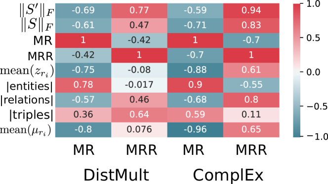
Figure 9: Spearman correlation of accuracy performance to structural descriptors of knowledge graphs.

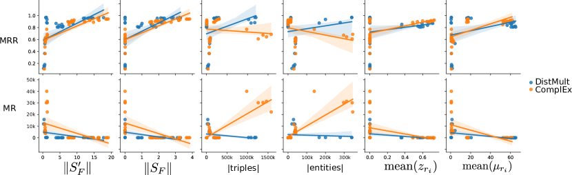
Figure 10: Regression plots detailing the linear correlation of the performance of a model to structural descriptors of knowledge graphs.

In the following we use the abbreviation corr to refer to the Spearman correlation (since distributions are potentially not normal) of the MRR metric to intrinsic properties of graphs (Figure 9). We see that ComplEx depends on properties that emphasize semantic similarity among the relations (corr to $\lVert S^{\prime}\rVert_{F}\text{ at }0.94$ and to $\lVert S\rVert_{F}\text{ at }0.83$), it performs better whenever the graph has semantically related relations (be it dense or sparse), and it depends less on the number of triples (samples, corr 0.11), suggesting that this model better learns semantic relationships within the graph. On the other hand, DistMult leverages less the role equivalence similarity (corr to $\lVert S\rVert_{F}=0.47$), concentrates more on similar entities (corr to $\lVert S^{\prime}\rVert_{F}=0.77$), and is highly sensitive to the number of triples (corr to $\sum_{r_{i}}|Pos|_{r_{i}}$ 0.64). This may explain why ComplEx outperforms DistMult at a small and extremely dense UMLS graph, and at a relatively big and sparse WN11 graph. DistMult, on the other hand, better leverages the abundant presence of triples in the big and sparse BIO-KG graph, and in the dense FB15k-237 graph. By looking at the regression plots (Figure 10), we can see that both models have high variability (small confidence) for the graphs that exhibit low semantic similarity among the relations, and contain very few samples at their disposal. Overall, the ComplEx model is better at extracting semantic relationships, while DistMult is better at leveraging big sample sizes.

6 Conclusions

The lessons learned from our experiments lead us to conclude that neural embeddings’ performance depends on the degree of how tight the relations within the knowledge graph interconnect entities. The presence of multiple relations – edges – that make the overall spider web of entities more entangled, affect the accuracy. Therefore, to increase the accuracy of neural embeddings in knowledge bases we would identify two main ingredients: a) increase the sample size, b) add similar relations. Obviously, by introducing novel relation types we increase the overall sample size. The addition of semantically similar relations can be achieved by using logical reasoners, or by recurring to external data sources. For instance, language models could be used to augment knowledge bases [29].

Herein, we proposed an open-source evaluation benchmark for knowledge graph embeddings that better captures structural variability and its change in real world knowledge graphs.

References

-
[1]
D. Liben-Nowell, J. Kleinberg,
The link
prediction problem for social networks, in: Proceedings of the twelfth
international conference on Information and knowledge management - CIKM
’03, ACM Press, New York, New York, USA, 2003, p. 556.
doi:10.1145/956863.956972.
URL http://portal.acm.org/citation.cfm?doid=956863.956972 -
[2]
M. Nickel, K. Murphy, V. Tresp, E. Gabrilovich,
A review of relational
machine learning for knowledge graphs, Proc. IEEE 104 (1) (2016) 11–33.
doi:10.1109/JPROC.2015.2483592.
URL http://ieeexplore.ieee.org/document/7358050/ - [3] S. Sri Nurdiati, C. Hoede, 25 years development of knowledge graph theory: the results and the challenge, no. 2/1876 in Memorandum, Discrete Mathematics and Mathematical Programming (DMMP), 2008.
-
[4]
T. Mikolov, I. Sutskever, K. Chen, G. Corrado, J. Dean,
Distributed representations of words
and phrases and their compositionality, arXiv.
URL https://arxiv.org/abs/1310.4546 -
[5]
P. Goyal, E. Ferrara,
Graph
embedding techniques, applications, and performance: A survey,
Knowledge-Based Systems 151 (2018) 78 – 94.
doi:https://doi.org/10.1016/j.knosys.2018.03.022.
URL http://www.sciencedirect.com/science/article/pii/S0950705118301540 - [6] A. Bordes, N. Usunier, A. Garcia-Duran, J. Weston, O. Yakhnenko, Translating embeddings for modeling multi-relational data, in: Proc. NIPS 2013, 2013.
- [7] B. Yang, S. W.-t. Yih, X. He, J. Gao, L. Deng, Embedding entities and relations for learning and inference in knowledge bases, in: Proc. of ICLR, 2015.
- [8] T. Trouillon, J. Welbl, S. Riedel, E. Gaussier, G. Bouchard, Complex embeddings for simple link prediction, in: Proc. of ICML, 2016, pp. 2071–2080.
-
[9]
R. Kadlec, O. Bajgar, J. Kleindienst,
Knowledge base completion: Baselines
strike back, arXiv:1705.10744 [cs].
URL http://arxiv.org/abs/1705.10744 -
[10]
L. Wu, A. Fisch, S. Chopra, K. Adams, A. Bordes, J. Weston,
Starspace: Embed all the things!,
arXiv.
URL https://arxiv.org/abs/1709.03856 -
[11]
M. Nickel, D. Kiela, Poincaré
embeddings for learning hierarchical representations, arXiv:1705.08039
[cs, stat].
URL http://arxiv.org/abs/1705.08039 -
[12]
B. Perozzi, R. Al-Rfou, S. Skiena,
Deepwalk: Online
learning of social representations, in: Proceedings of the 20th ACM SIGKDD
international conference on Knowledge discovery and data mining - KDD ’14,
ACM Press, New York, New York, USA, 2014, pp. 701–710.
doi:10.1145/2623330.2623732.
URL http://dl.acm.org/citation.cfm?doid=2623330.2623732 -
[13]
A. Grover, J. Leskovec,
node2vec: Scalable feature
learning for networks., KDD 2016 (2016) 855–864.
doi:10.1145/2939672.2939754.
URL http://dx.doi.org/10.1145/2939672.2939754 -
[14]
D. Garcia-Gasulla, E. Ayguadé, J. Labarta, U. Cortés,
Limitations and alternatives for the
evaluation of large-scale link prediction, arXiv.
URL https://arxiv.org/abs/1611.00547 -
[15]
B. P. Chamberlain, J. Clough, M. P. Deisenroth,
Neural embeddings of graphs in
hyperbolic space, arXiv:1705.10359 [cs, stat].
URL http://arxiv.org/abs/1705.10359 -
[16]
M. Alshahrani, M. A. Khan, O. Maddouri, A. R. Kinjo, N. Queralt-Rosinach,
R. Hoehndorf,
Neuro-symbolic
representation learning on biological knowledge graphs., Bioinformatics
33 (17) (2017) 2723–2730.
doi:10.1093/bioinformatics/btx275.
URL http://dx.doi.org/10.1093/bioinformatics/btx275 -
[17]
A. Agibetov, M. Samwald, Global and
local evaluation of link prediction tasks with neural embeddings, arXiv.
URL https://arxiv.org/abs/1807.10511 -
[18]
G. Crichton, Y. Guo, S. Pyysalo, A. Korhonen,
Neural networks for link
prediction in realistic biomedical graphs: a multi-dimensional evaluation of
graph embedding-based approaches., BMC Bioinformatics 19 (1) (2018) 176.
doi:10.1186/s12859-018-2163-9.
URL http://dx.doi.org/10.1186/s12859-018-2163-9 -
[19]
K. Toutanova, V. Lin, W.-t. Yih, H. Poon, C. Quirk,
Compositional learning of
embeddings for relation paths in knowledge base and text, in: Proceedings of
the 54th Annual Meeting of the Association for Computational Linguistics
(Volume 1: Long Papers), Association for Computational Linguistics,
Stroudsburg, PA, USA, 2016, pp. 1434–1444.
doi:10.18653/v1/P16-1136.
URL http://aclweb.org/anthology/P16-1136 -
[20]
T. Dettmers, P. Minervini, P. Stenetorp, S. Riedel,
Convolutional 2D knowledge graph
embeddings.
URL https://arxiv.org/abs/1707.01476 - [21] S. Y. Yu, S. Rokka Chhetri, A. Canedo, P. Goyal, M. A. A. Faruque, Pykg2vec: A python library for knowledge graph embedding, arXiv preprint arXiv:1906.04239.
- [22] M. Ali, C. T. Hoyt, D. Domingo-Fernández, J. Lehmann, Predicting missing links using pykeen, in: Proceedings of the ISWC 2019 Satellite Tracks (Posters & Demonstrations, Industry, and Outrageous Ideas), Vol. 2456 of CEUR Workshop Proceedings, CEUR-WS.org, 2019, pp. 245–248.
- [23] P. Goyal, D. Huang, A. Goswami, S. R. Chhetri, A. Canedo, E. Ferrara, Benchmarks for graph embedding evaluation, arXiv abs/1908.06543.
-
[24]
G. A. Miller,
WordNet: a
lexical database for english, Commun ACM 38 (11) (1995) 39–41.
doi:10.1145/219717.219748.
URL http://portal.acm.org/citation.cfm?doid=219717.219748 -
[25]
K. Bollacker, C. Evans, P. Paritosh, T. Sturge, J. Taylor,
Freebase: A
collaboratively created graph database for structuring human knowledge, in:
Proceedings of the 2008 ACM SIGMOD international conference on Management of
data - SIGMOD ’08, ACM Press, New York, New York, USA, 2008, p. 1247.
doi:10.1145/1376616.1376746.
URL http://portal.acm.org/citation.cfm?doid=1376616.1376746 - [26] O. Bodenreider, The unified medical language system (UMLS): integrating biomedical terminology., Nucleic Acids Res 32 (Database issue) (2004) D267–70. doi:10.1093/nar/gkh061.
-
[27]
F. Pedregosa, G. Varoquaux, A. Gramfort, V. Michel, B. Thirion, O. Grisel,
M. Blondel, P. Prettenhofer, R. Weiss, V. Dubourg, J. Vanderplas, A. Passos,
D. Cournapeau, M. Brucher, M. Perrot, E. Duchesnay,
Scikit-learn:
Machine learning in python, Journal of Machine Learning Research.
URL http://jmlr.csail.mit.edu/papers/v12/pedregosa11a.html - [28] W. McKinney, Data structures for statistical computing in python, in: S. van der Walt, J. Millman (Eds.), Proceedings of the 9th Python in Science Conference, 2010, pp. 51 – 56.
- [29] F. Petroni, T. Rocktäschel, S. Riedel, P. S. H. Lewis, A. Bakhtin, Y. Wu, A. H. Miller, Language models as knowledge bases?, in: Proc. EMNLP-IJCNLP Conference, Association for Computational Linguistics, 2019, pp. 2463–2473.