Stochastic interpolation of sparsely sampled time series via multi-point fractional Brownian bridges

Abstract

We propose and test a method to interpolate sparsely sampled signals by a stochastic process with a broad range of spatial and/or temporal scales. To this end, we extend the notion of a fractional Brownian bridge, defined as fractional Brownian motion with a given scaling (Hurst) exponent $H$ and with prescribed start and end points, to a bridge process with an arbitrary number of intermediate and non-equidistant points. Determining the optimal value of the Hurst exponent, $H_{opt}$, appropriate to interpolate the sparse signal, is a very important step of our method. We demonstrate the validity of our method on a signal from fluid turbulence in a high Reynolds number flow and discuss the implications of the non-self-similar character of the signal. The method introduced here could be instrumental in several physical problems, including astrophysics, particle tracking, specific tailoring of surrogate data, as well as in domains of natural and social sciences.

Many non-equilibrium phenomena in physics involve random fluctuations with a wide range of spatial and/or temporal scales [1, 2]. The theory of stochastic processes provides a conceptual framework to describe such phenomena [3, 4]. The most emblematic example is provided by Brownian motion, which results from random uncorrelated collisions acting on a particle, and can be described by a Wiener process [5]. Nonetheless, several complex systems in nature [6, 7, 8, 9, 10, 11] also involve long- or short-range correlations which can be described in terms of fractional Brownian motion [12, 13]. Furthermore, the description of a broad range of problems in physics or in the general field of complex systems requires the fractional Brownian motion (fBm) process to be constrained, by passing through a certain number of prescribed points. Typical examples include the tracking of animal movement [14], information-based financial models [15], the number of neutrons involved in reactor diffusion [16, 17], or cosmic ray propagation in astrophysical turbulence [18].

Current stochastic interpolation methods, e.g., kriging [19, 20], which is used for data reconstruction/spatial enhancement of particle image velocimetry [21], interpolations of buoy location in the tropical pacific [22], and interpolation of rainfall data from rain gages and radars [23, 24], or other various types of polynomial interpolation act often to smooth the underlying data [25]. A more promising method to interpolate sparse data sets has been introduced in the field of surface hydrology [26, 27], using the Lévy-Ciesielski construction [12, 28]. This construction, however, is exact only in the very special case when the random processes are describable by ordinary Brownian motion [29, 30].

Providing a more faithful representation of the data requires the development of exact stochastic interpolations on the basis of fBm while at the same time giving an estimate for the optimal Hurst exponent which characterizes the roughness of the sparsely sampled data.

Here, we stress the important example of cosmic ray propagation in turbulent magnetic fields [31, 32]. In order to overcome the overwhelming problem of resolving the wide range of scales involved in these extremely high Reynolds number astrophysical flows, several methods for generating synthetic turbulent fields were developed in the last decades [33, 34, 35, 36]. Such methods are frequently implemented and used in major cosmic ray propagation codes (see e.g. [18]). To capture large anisotropies due to the geometry of galaxies (spiral arms, outflow regions, bow shocks), synthetic turbulent fields must be embedded in large-scale magnetohydrodynamic (MHD) simulations of the turbulent interstellar or intergalactic plasma. Therefore, in this problem we face two challenges: i.) fBm, which is used to emulate turbulent flow properties, must be constrained to match the values on the numerical grid of the MHD simulation and ii.) scaling properties, represented by the Hurst exponent of fluctuations of the coarse-grained MHD simulation must be determined from sparse grid data, in order to allow for an “optimal stochastic interpolation” of sparsely-sampled data.

In the following, we will restrict ourselves to temporal processes, or more generally to processes depending on only one variable. The fBm $X(t)$ is a nonstationary centered Gaussian process, and thus entirely characterized by its covariance

$$\langle X(t)X(t^{\prime})\rangle=\frac{1}{2}\left(|t|^{2H}+|t^{\prime}|^{2H}-|t-t^{\prime}|^{2H}\right)\;.$$ (1)

which implies that $\langle(X(t)-X(t^{\prime}))^{2}\rangle=|t-t^{\prime}|^{2H}$, where $H$ denotes the Hurst exponent. We first present a method to construct a fBm $X(t)$, which takes specific values $X_{i}$ at times $t_{i}$, and subsequently discuss its application as an optimal stochastic interpolation of a sparsely-sampled real time signal. Accordingly, we start with the well-known notion of a fractional Brownian bridge [37, 38, 39], which is defined as fBm starting from zero at $t=0$, ending at $X_{1}$ at $t=t_{1}$, and possessing the same statistical (including scaling (1)) properties as $X(t)$. Such a fractional Brownian bridge (fBb) can be constructed from $X(t)$ according to

$$X^{B}(t)=X(t)-(X(t_{1})-X_{1})\frac{\langle X(t)X(t_{1})\rangle}{\langle X(t_{1})^{2}\rangle}\;.$$ (2)

It is possible to generalize this ordinary fBb to an arbitrary number of prescribed intermediate grid points in the following manner: First, we consider the $n$-times conditional moments

$$\langle X(t)|\{X_{i},t_{i}\}\rangle= \frac{\langle X(t)\prod_{i=1}^{n}\delta(X(t_{i})-X_{i})\rangle}{\prod_{i=1}^{n}\langle\delta(X(t_{i})-X_{i})\rangle}\;,$$ (3)

$$\langle X(t)X(t^{\prime})|\{X_{i},t_{i}\}\rangle= \frac{\langle X(t)X(t^{\prime})\prod_{i=1}^{n}\delta(X(t_{i})-X_{i})\rangle}{\prod_{i=1}^{n}\langle\delta(X(t_{i})-X_{i})\rangle}\;.$$ (4)

We then demand that our bridge process $X^{B}(t)$ is conditional on $X_{i}$ at $t_{i}$ for $i=1,\ldots,n$, which is equivalent to the process possessing the conditional moments (3-4). For a Gaussian process with zero mean and covariance $\langle X(t)X(t^{\prime})\rangle$, the conditional moments read

$$\langle X(t)|\{X_{i},t_{i}\}\rangle=\left\langle X(t)X(t_{i})\right\rangle\sigma_{ij}^{-1}X_{j}\;,$$ (5)

and

$$\langle X(t)X(t^{\prime})|\{X_{i},t_{i}\}\rangle=\left\langle X(t)X(t^{\prime})\right\rangle$$ (6)

$$~{}~{}-\left\langle X(t)X(t_{i})\right\rangle\left[\sigma_{ij}^{-1}-\sigma_{ik}^{-1}X_{k}X_{l}\sigma_{jl}^{-1}\right]\left\langle X(t^{\prime})X(t_{j})\right\rangle\;,$$

where we implied summation over equal indices and where $\sigma_{ij}=\langle X(t_{i})X(t_{j})\rangle$ denotes the covariance matrix. As shown in [40], the multi-point fractional Brownian bridge

$$X^{B}(t)=X(t)-(X(t_{i})-X_{i})\sigma_{ij}^{-1}\left\langle X(t)X(t_{j})\right\rangle\;,$$ (7)

possesses one- and two-point moments which are identical to (5-6) and we thus conclude that $X^{B}(t)$ is the stochastic process $X(t)$ conditioned on points $X_{i}$ at times $t_{i}$. We indeed obtain $X^{B}(t_{k})=X(t_{k})-(X(t_{i})-X_{i})\sigma_{ij}^{-1}\sigma_{jk}=X(t_{k})-(X(t_{i})-X_{i})\delta_{ik}=X_{k}$. Fig. 1(a) depicts the multi-point fBb (7) for three different Hurst exponents with $16$ equidistant fixed points (black). Here, fBm realizations $X(t)$ were generated by the Davies-Harte method [53], which is an exact numerical implementation of fBm (by contrast to other methods, e.g., Fourier representations; see also [40] for further specifications).

Figure 1: (a) Multi-point fractional Brownian bridge (7) for different Hurst exponents $H$ but identical grid points (black). The $16$ equidistant grid points $(t_{i},X_{i})$ were drawn randomly from the interval $X_{i}\in[-0.5,0.5]$. The full temporal resolution comprises $4096$ points and the inset zooms into the vicinity of one of the prescribed points. (b) Second order structure function $S_{2}(\tau)=\langle(X^{B}(t+\tau)-X^{B}(t))^{2}\rangle$ calculated from $100$ realizations of the multi-point fractional Brownian bridge (7) for $N=32768$ total grid points and $\tilde{N}=32$ prescribed grid points. Dashed lines correspond to the explicit formula (8), whereas thin grey lines correspond to the ordinary scaling of fBm $|\tau|^{2H}$ and extend up to the grid length of the coarse grid $\textrm{d}\tilde{t}=1/32$. The prescribed grid points were drawn as fBm with $\tilde{H}=0.5$. Accordingly, the fBb with $H=0.5$ (orange curve) is the optimal bridge that belongs to the prescribed points. (c) Cost curve $H_{emp}(H)-H$ for three under-sampled time series $\tilde{N}=128$ (fBm with $\tilde{H}=0.33,0.5,0.66$ for samples 1-3). Each time series is embedded into bridges (7) with varying Hurst exponents $H$ and resolution $N=4096$. Therefore, the fit for $H_{emp}$ relies on the left part of (b).

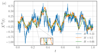
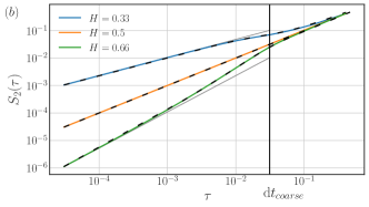
In order to check that the simulated bridge processes possess the desired properties (1) and (5-6), we have carried out numerical calculations of the second order structure functions $S_{2}(\tau)=\left\langle(X^{B}(t+\tau)-X^{B}(t))^{2}\right\rangle$ for three different Hurst exponents ($H=0.33,0.5,0.66$) with a total number of $N=32768$ total grid points. From these we prescribed $\tilde{N}=32$ equidistant points generated from fBm (1) with a Hurst exponent $\tilde{H}=0.5$. The results are shown in Fig. 1(b) and are in agreement with the prediction $S_{2}(\tau)=|\tau|^{2H}$ (dashed black lines) for small $\tau$. For such a case, where the prescribed points also follow fBm with Hurst exponent $\tilde{H}$, we can obtain an explicit formula for $S_{2}(\tau)$ from Eq. (7), namely

$$S_{2}(\tau)=|\tau|^{2H}$$ (8)

$$-\langle\delta_{\tau}X(t)X(t_{i})\rangle\left[\sigma_{ij}^{-1}-\sigma_{ik}^{-1}\tilde{\sigma}_{kl}\sigma_{lj}^{-1}\right]\langle\delta_{\tau}X(t)X(t_{j})\rangle\;,$$

where $\delta_{\tau}X(t)=X(t+\tau)-X(t)$ and where $\tilde{\sigma}_{ij}=\langle X_{i}X_{j}\rangle$ denotes the covariance matrix of the prescribed points with $\tilde{H}$. Consequently, $H=\tilde{H}$ implies $\sigma=\tilde{\sigma}$, which yields $S_{2}(\tau)=|\tau|^{2H}$. Hence, Eq. (8) entails that strict self-similarity of the multi-point fBb is only guaranteed if the bridge fBm process $X(t)$ characterized by $H$ matches the Hurst exponent $\tilde{H}$ of the prescribed points $X_{i}$. Other bridge multi-point fBbs with $H\neq\tilde{H}$ correspond to multifractional Brownian motion with a time-dependent Hurst exponent, as shown in Fig. 1(b) (we also refer to [54, 55] for further references). In other words, given a certain time series $\{X_{i},t_{i}\}$ that possesses a self-similar part governed by $\tilde{H}$, the bridge with $H=\tilde{H}$ can be considered as the optimal stochastic interpolation of this time series.

Therefore, as already highlighted in the introduction, we are now in the position to describe an optimization procedure that allows estimating Hurst exponents from sparsely sampled time series. The basic idea is to embed a given time series $\{X_{i},t_{i}\}$ into fBbs (7) with varying Hurst exponents $H$. For each of these bridges we determine the empirical Hurst exponent $H_{emp}$ as a function of $H$ by fitting the second order structure function up to the smallest time scale of the time series $\textrm{d}\tilde{t}$, (i.e., fitting only the left part up to $\textrm{d}t_{coarse}$ in Fig. 1(b)). This procedure ensures that we only measure deviations from the scaling $|\tau|^{2H}$ in the interpolated region (grey lines in Fig. 1(b)) and are not directly contaminated by correlations contained in $\{X_{i},t_{i}\}$.

Figure 2: (a) Turbulent velocity field measurements (blue) in a von Kármán experiment using normal Helium. The number of points $N=16384$ corresponds roughly to one integral length scale $L$. The corresponding fBb (orange) was constructed from $\tilde{N}=64$ points of the signal (black) and possesses a resolution of $1024$ points. The smallest scale of the bridge process therefore corresponds approximately to the Taylor scale of the flow which ensures that the fBb and the velocity field $u(x)$ possess comparable inertial ranges. Small-scale turbulent fluctuations in the velocity field (blue) cannot be reproduced by the fBb due to its restricting Gaussian properties. The Hurst exponent for the fBb $H=0.376$ was determined from randomized samples of the original turbulent signal such as the one depicted in (b). Due to the self-similarity of these samples, an optimization procedure similar to the one depicted in Fig. 1(c) could be applied. The bridge (orange) is in much better agreement with the self-similar signal (blue) in (b) than with the original signal (blue) in (a).

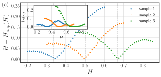
We have tested our optimization for three different samples of fBm with Hurst exponents $\tilde{H}=0.33,0.5,0.66$ and $\tilde{N}=128$ grid points. Each of the samples was embedded in fBbs with varying Hurst exponents $H$ and $N=4096$ grid points. Fig. 1(c) depicts the minimization of $H_{emp}(H)$ for the three samples. It can be clearly seen that optimal Hurst exponents $H_{opt}$ are recovered with high accuracy, although slight variations ($\Delta H_{opt}\approx 0.015$ from 20 different samples of the same $\tilde{H}$) between different samples can be observed [40]. This effect can be attributed to finite sample sizes, and the corresponding deviations remain rather small, which is quite appealing given the fact that common methods (rescaled range analysis [56] or wavelets [57]) yield erroneous results for such sparsely sampled time series. The proposed method can thus roughly be considered as the extrapolation of self-similar properties of a given time series to finer scales.

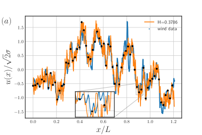
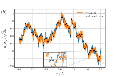
In the examples discussed so far, we have systematically chosen the synthetic signal $X_{i}$, as well as the process $X(t)$ used in Eqs. (1,7), to be normalized in the same manner. In order to apply our optimization to real signals, we examine a turbulent velocity time series obtained from hot wire anemometry in the superfluid high Reynolds von Kármán experiment (SHREK) at CEA-Grenoble [58]. The particular experimental setup is a von Kármán cell with two-counter rotating disks (-0.12 Hz on top, +0.18 Hz on bottom) in normal Helium (see [59] for further specifications). The temporal resolution is 50kHz and the attained Taylor-Reynolds number was $\textrm{Re}_{\lambda}=2737$. We applied Taylor’s hypothesis of frozen turbulence [60] to relate single-point velocity measurement at time $t$ to scales $x=\langle u\rangle t$, where $\langle u\rangle$ is the mean velocity. Furthermore, a key prerequisite for the above mentioned optimization procedure is the standardization of the signal by $\lim_{r\rightarrow L}\sqrt{\left\langle(u(x+r)-u(x))^{2}\right\rangle}=\sqrt{2\left\langle u(x))^{2}\right\rangle}=\sqrt{2}\sigma$. This standardization ensures the correct large-scale limit of the second-order structure function in Fig. 1(b), which was necessarily fulfilled by the synthetic samples of fBm (1) in the previous study. The blue curve in Fig. 2(a) depicts an extract of the velocity field $u(x)$ standardized by $\sigma$ of the total signal for around one integral length scale $L$.

By contrast to the above optimization procedure for data from synthetic samples, the present analysis is complicated by: i.) the existence of different scaling regimes in the flow, namely a dissipative and integral range of scales, and ii.) non-self similar (intermittent) features in the signal. Turning to point i.), we chose sample sizes of length $L$ and determined the subset of points in order to guarantee that their grid length lies within the inertial range of scales (here we choose $\approx 100\eta$). As far as point ii.) is concerned, intermittent features manifest themselves in form of strongly varying $H_{opt}$ for different samples [40]. An example of such an intermittent fluctuation is well visible in the signal shown in Fig. 2(a), at $x\approx 0.8L$. In this region our interpolation procedure does not work very well and the bridge process (7) has to be generalized to a non-Gaussian process. In this letter, however, we are solely interested in the self-similar part of the signal and thus perform a randomization of Fourier phases of the turbulent signal. A snapshot of the resulting randomized signal is depicted in Fig. 2(b). Strikingly, and contrary to Fig. 2(a), our interpolation procedure leads to much better results than for the original signal. The randomization procedure has effectively suppressed intermittency, and made the signal essentially Gaussian. We fed several samples of this randomized signal into our optimization routine which reduced fluctuations of the Hurst exponent to an extend comparable to the ones observed in synthetic signals [40]. Moreover, we obtain a Hurst exponent of the randomized signal $H_{opt}=0.3786\pm 0.0251$ (evaluated from the optimization of 100 snapshots [40]). To put this result into context, we consider the log-normal model of turbulence [49, 50] which suggests scaling exponents $\zeta_{n}=n/3-\mu n(n-3)/18$ for the scaling of structure functions $\langle(u(x+r)-u(x))^{n}\rangle\sim|r|^{\zeta_{n}}$ where $\mu$ denotes the intermittency coefficient. Hence, the self-similar part in the K62 model is given by $H_{K62}=(2+\mu)/6$ and can be compared to our analysis. The above mentioned value from the optimization procedure of the randomized signal $H_{opt}=0.3786\pm 0.0251$ thus suggests that $\mu=0.2716\pm 0.1506$. Latter value for the intermittency coefficient is comparable to $\mu=0.2913\pm 0.0853$ acquired from an analysis of the entire turbulent signal [40]. It is thus important to stress here, that the combination of both the Fourier phase randomization and the optimization procedure via the multi-point fBbs is capable of reproducing the monofractal/self-similar part of the turbulent signal, which is also strongly supported by Fig. 2(b).

To conclude, we have presented a generalization of a fractional Brownian bridge to a stochastic process with an arbitrary number of prescribed points. Furthermore, we devised an optimization method which allowed us to estimate the Hurst exponent of a sparsely sampled time series. Our method has proven reliable even in the presence of strong anomalous fluctuations, i.e., non-self-similar features, at small scales. In order to address such features, which are visibly not captured by the multi-point fBb in Fig. 2(a), it will be a task for the future to construct multi-point bridge processes with multiscaling properties (i.e., which are non-self-similar and potentially possess a dissipative scale [61, 62, 63, 64, 65]). A generalization of the bridge process (7) to an arbitrary number of dimensions is straight-forward and might be of potential interest for the construction of various synthetic fields in several physical contexts. In turbulence, the full spatio-temporal (though non-intermittent) Eulerian velocity field $\mathbf{u}(\mathbf{x},t)$ can possibly be reconstructed from a set of Lagrangian trajectories $\mathbf{X}(\mathbf{y},t)$ where $\mathbf{\dot{X}}(\mathbf{y},t)=\mathbf{u}(\mathbf{X}(\mathbf{y},t),t)$. Such applications could be of considerable interest for particle tracking measurements, which sometimes require a certain knowledge of the flow field in the vicinity of tracer particles [66]. Furthermore, the optimization procedure may help to shed light into the ongoing discussion about the inertial range power spectrum in the solar wind [67, 9]. To this end, the ideas proposed in this work should be extended to take into account the existence of several ranges of scales, involving different power law behaviors [40]. Last, we mention possible extensions of our method which might apply or even improve concepts borrowed from machine learning [68, 69, 70, 71]. Moreover, the prior assignment of hot- and cold-spot clusters by a simple $k$-means algorithm might be suitable to model land price fields by multi-point fractional Brownian scalar fields in the widely different domain of urban decision making [72].

We are grateful to the SHREK collaboration [58, 59] for providing us with their hot wire anemometry measurements. J.F. acknowledges funding from the Humboldt Foundation within a Feodor-Lynen fellowship and also benefited from financial support of the Project IDEXLYON of the University of Lyon in the framework of the French program “Programme Investissements d’Avenir” (ANR-16-IDEX-0005). S.G.’s visit to Lyon was financially supported by the German Academic Exchange Service through a PROMOS scholarship.

References

- Haken [1983] H. Haken, Synergetics, An Introduction (Springer, Berlin, Heidelberg, 1983).
- Prigogine [1987] I. Prigogine, Eur. J. Oper. Res. 30, 97 (1987).
- Wax [1954] N. Wax, Noise and stochastic processes (Dover Publications, 1954).
- Friedrich et al. [2011] R. Friedrich, J. Peinke, M. Sahimi, and R. M. Tabar, Phys. Rep. 506, 87 (2011).
- Einstein [1905] A. Einstein, Ann. Phys. 17, 549 (1905).
- Kolmogorov [1941] A. N. Kolmogorov, Dokl. Akad. Nauk Sssr 30, 301 (1941).
- Onsager [1949] L. Onsager, Nuovo Cim. 6, 279 (1949).
- v. Weizsäcker [1948] C. F. v. Weizsäcker, Zeitschrift für Phys. 124, 614 (1948).
- Goldstein et al. [1995] M. L. Goldstein, D. A. Roberts, and W. Matthaeus, Annu. Rev. Astron. Astrophys. 33, 283 (1995).
- Makarava et al. [2014] N. Makarava, S. Menz, M. Theves, W. Huisinga, C. Beta, and M. Holschneider, Phys. Rev. E 90, 042703 (2014).
- Peng et al. [1993] C.-K. Peng, J. Mietus, J. M. Hausdorff, S. Havlin, H. E. Stanley, and A. L. Goldberger, Phys. Rev. Lett. 70, 1343 (1993).
- Lévy and Loeve [1965] P. Lévy and M. Loeve, Processus stochastiques et mouvement brownien (Gauthier-Villars Paris, 1965).
- Mandelbrot and Ness [1968] B. B. Mandelbrot and J. W. V. Ness, SIAM Review 10, 422 (1968).
- Kranstauber et al. [2012] B. Kranstauber, R. Kays, S. D. LaPoint, M. Wikelski, and K. Safi, J. Anim. Ecol. 81, 738 (2012).
- Brody et al. [2008] D. C. Brody, L. P. Hughston, and A. Macrina, Int. J. Theor. Appl. Finance 11, 107 (2008).
- de Mulatier et al. [2015] C. de Mulatier, E. Dumonteil, A. Rosso, and A. Zoia, J. Stat. Mech: Theory Exp. 2015, P08021 (2015).
- Mazzolo [2017a] A. Mazzolo, J. Stat. Mech: Theory Exp. 2017, 023203 (2017a).
- Batista et al. [2016] R. A. Batista, A. Dundovic, M. Erdmann, K.-H. Kampert, D. Kuempel, G. Müller, G. Sigl, A. van Vliet, D. Walz, and T. Winchen, J. Cosmol. Astropart. Phys. 2016, 038 (2016).
- Cressie [1990] N. Cressie, Mathematical geology 22, 239 (1990).
- Delhomme [1978] J. Delhomme, Advances in Water Resources 1, 251 (1978).
- Gunes and Rist [2008] H. Gunes and U. Rist, Phys. Fluids 20, 104109 (2008).
- Hansen and Herman [1989] D. V. Hansen and A. Herman, Journal of Atmospheric and Oceanic Technology 6, 599 (1989).
- Seo et al. [1990a] D.-J. Seo, W. F. Krajewski, A. Azimi-Zonooz, and D. S. Bowles, Water. Resour. Res. 26, 915 (1990a).
- Seo et al. [1990b] D.-J. Seo, W. F. Krajewski, and D. S. Bowles, Water. Resour. Res. 26, 469 (1990b).
- Griffa et al. [2004] A. Griffa, L. I. Piterbarg, and T. Özgökmen, J. Mar. Res. 62, 1 (2004).
- Molz and Boman [1993] F. J. Molz and G. K. Boman, Water. Resour. Res. 29, 3769 (1993).
- Molz et al. [1997] F. Molz, H. Liu, and J. Szulga, Water. Resour. Res. 33, 2273 (1997).
- Ciesielski [1961] Z. Ciesielski, Trans. Amer. Math. Soc. , 403 (1961).
- Saupe [1988] D. Saupe, in The science of fractal images (Springer, 1988) pp. 71–136.
- Voss [1988] R. F. Voss, The Science of Fractal Images , 21 (1988).
- Schlickeiser [2015] R. Schlickeiser, Phys. Plasmas 22, 091502 (2015).
- Zweibel [2013] E. G. Zweibel, Phys. Plasmas 20, 055501 (2013).
- Giacalone and Jokipii [1999] J. Giacalone and J. R. Jokipii, ApJ 520, 204 (1999).
- Zimbardo et al. [2015] G. Zimbardo, E. Amato, A. Bovet, F. Effenberger, A. Fasoli, H. Fichtner, I. Furno, K. Gustafson, P. Ricci, and S. Perri, J. Plasma Phys. 81, 495810601 (2015).
- Snodin et al. [2016] A. P. Snodin, A. Shukurov, G. R. Sarson, P. J. Bushby, and L. F. S. Rodrigues, MNRAS 457, 3975 (2016).
- Reichherzer et al. [2019] P. Reichherzer, J. Becker Tjus, E. G. Zweibel, L. Merten, and M. J. Pueschel, arXiv e-prints , arXiv:1910.07528 (2019).
- Delorme and Wiese [2016] M. Delorme and K. J. Wiese, Phys. Rev. E 94, 052105 (2016).
- Sottinen and Yazigi [2014] T. Sottinen and A. Yazigi, Stochastic Processes Appl. 124, 3084 (2014).
- Walter and Wiese [2020] B. Walter and K. J. Wiese, Phys. Rev. E 101 (2020).
- [40] See Supplemental Material, which includes Refs. [41-52], for further discussion and proofs.
- Lim and Muniandy [2002] S. C. Lim and S. V. Muniandy, Phys. Rev. E 66, 021114 (2002).
- Grebenkov et al. [2015] D. S. Grebenkov, D. Belyaev, and P. W. Jones, Journal of Physics A: Mathematical and Theoretical 49, 043001 (2015).
- Beran [1994] J. Beran, Statistics for long-memory processes, Vol. 61 (CRC press, 1994).
- Flandrin [1989] P. Flandrin, IEEE Transactions on information theory 35, 197 (1989).
- [45] https://pypi.org/project/fbm/.
- Risken [1996] H. Risken, The Fokker-Planck Equation (Springer, Berlin, 1996).
- Mazzolo [2017b] A. Mazzolo, J. Math. Phys. 58, 093302 (2017b).
- Stevens [1995] C. F. Stevens, The six core theories of modern physics (MIT Press, 1995).
- Kolmogorov [1962] A. N. Kolmogorov, J. Fluid Mech. 13, 82 (1962).
- Oboukhov [1962] A. M. Oboukhov, J. Fluid Mech. 67, 77 (1962).
- Friedrich and Peinke [1997] R. Friedrich and J. Peinke, Phys. Rev. Lett. 78, 863 (1997).
- Yakhot [2006] V. Yakhot, Phys. D 215, 166 (2006).
- Davies and Harte [1987] R. B. Davies and D. S. Harte, Biometrika 74, 95 (1987).
- Peltier and Véhel [1995] R.-F. Peltier and J. L. Véhel, INRIA, Project 2645 (1995).
- Benassi et al. [1997] A. Benassi, D. Roux, and S. Jaffard, Rev. Mat. Iberoam. 13, 19 (1997).
- Caccia et al. [1997] D. C. Caccia, D. Percival, M. J. Cannon, G. Raymond, and J. B. Bassingthwaighte, Physica A 246, 609 (1997).
- Simonsen et al. [1998] I. Simonsen, A. Hansen, and O. M. Nes, Phys. Rev. E 58, 2779 (1998).
- Rousset et al. [2014] B. Rousset, P. Bonnay, P. Diribarne, A. Girard, J.-M. Poncet, E. Herbert, J. Salort, C. Baudet, B. Castaing, L. Chevillard, et al., Rev. Sci. Instrum. 85, 103908 (2014).
- Kharche et al. [2018] S. Kharche, M. Bon-Mardion, J.-P. Moro, J. Peinke, B. Rousset, and A. Girard, in iTi Conference on Turbulence (Springer, 2018) pp. 179–184.
- Monin and Yaglom [2007] A. S. Monin and A. M. Yaglom, Statistical Fluid Mechanics: Mechanics of Turbulence (Courier Dover Publications, 2007).
- Chevillard et al. [2019] L. Chevillard, C. Garban, R. Rhodes, and V. Vargas, in Annales Henri Poincaré, Vol. 20 (Springer, 2019) pp. 3693–3741.
- Viggiano et al. [2020] B. Viggiano, J. Friedrich, R. Volk, M. Bourgoin, R. B. Cal, and L. Chevillard, J. Fluid Mech. 900 (2020).
- Rosales and Meneveau [2008] C. Rosales and C. Meneveau, Phys. Rev. E 78, 016313 (2008).
- Juneja et al. [1994] A. Juneja, D. Lathrop, K. Sreenivasan, and G. Stolovitzky, Phys. Rev. E 49, 5179 (1994).
- Malara et al. [2016] F. Malara, F. Di Mare, G. Nigro, and L. Sorriso-Valvo, Phys. Rev. E 94, 053109 (2016).
- Machicoane et al. [2019] N. Machicoane, P. D. Huck, A. Clark, A. Aliseda, R. Volk, and M. Bourgoin, in Flowing Matter (Springer, 2019) pp. 177–209.
- Boldyrev [2005] S. Boldyrev, Astrophys. J. Lett. 626, L37 (2005).
- Brenner et al. [2019] M. Brenner, J. Eldredge, and J. Freund, Phys. Rev. Fluids 4, 100501 (2019).
- Jia and Ma [2017] Y. Jia and J. Ma, Geophysics 82, V163 (2017).
- Appelhans et al. [2015] T. Appelhans, E. Mwangomo, D. R. Hardy, A. Hemp, and T. Nauss, Spatial Statistics 14, 91 (2015).
- Rasmussen [2003] C. E. Rasmussen, in Summer School on Machine Learning (Springer, 2003) pp. 63–71.
- Lengyel and Friedrich [2020] J. Lengyel and J. Friedrich, “Multiscale urban modeling,” in Neue Dimensionen der Mobilität: Technische und betriebswirtschaftliche Aspekte, edited by H. Proff (Springer Fachmedien Wiesbaden, Wiesbaden, 2020) pp. 387–408.