Stochastic and Robust MPC for Bipedal Locomotion: A Comparative Study on Robustness and Performance

Abstract

Linear Model Predictive Control (MPC) has been successfully used for generating feasible walking motions for humanoid robots. However, the effect of uncertainties on constraints satisfaction has only been studied using Robust MPC (RMPC) approaches, which account for the worst-case realization of bounded disturbances at each time instant. In this letter, we propose for the first time to use linear stochastic MPC (SMPC) to account for uncertainties in bipedal walking. We show that SMPC offers more flexibility to the user (or a high level decision maker) by tolerating small (user-defined) probabilities of constraint violation. Therefore, SMPC can be tuned to achieve a constraint satisfaction probability that is arbitrarily close to 100%, but without sacrificing performance as much as tube-based RMPC. We compare SMPC against RMPC in terms of robustness (constraint satisfaction) and performance (optimality). Our results highlight the benefits of SMPC and its interest for the robotics community as a powerful mathematical tool for dealing with uncertainties.

I Introduction

Control of humanoid robots is challenging due to limiting constraints on contact forces, and nonlinear switching dynamics. Furthermore, guaranteeing safety for humanoids is critical, as collision with the environment or falling down can cause severe damage to the robot and its surroundings. Linear MPC [1][2] is a powerful tool for designing real-time feedback controllers subject to state and input constraints, which makes it a prime candidate for generating a wide range of feasible reference walking motions for humanoid robots [3, 4, 5]. However, the theoretical guarantees associated with MPC (e.g., constraint satisfaction guarantees) can easily be lost due to external disturbances or the discrepancy between the nonlinear dynamics of the robot and the linearized model used in control.

Recently, [6, 7] studied how to account for the bounded error in constraint satisfaction due to the approximation of the nonlinear center of mass (CoM) dynamics, and [8] investigated nonlinear constraints due to step timing adaptation. However, $1)$ they do not account for the closed-loop tracking errors due to disturbances, $2)$ there are no robustness guarantees of constraints satisfaction in the presence of different disturbances, which is critical for generating safe walking motions.

Linear Robust MPC (RMPC) schemes have been extensively studied in the control literature [9, 10, 11]. Recently, [12] used the well-known tube-based RMPC approach originally developed in [11] for generating robust walking motions for humanoid robots, taking into account the effects of additive compact polytopic uncertainties on the dynamics. Using a state feedback control policy and a pre-stabilizing choice of static dead-beat gains, they showed that constraints are guaranteed to be satisfied for all disturbance realizations inside the disturbance set. A drawback of RMPC is that the constraints are designed to accommodate for the worst-case disturbance, which is quite conservative and sacrifices performance (optimality) to guarantee hard constraints satisfaction.

In order to relax the conservativeness of RMPC, SMPC [13, 14, 15, 16] exploits the underlying probability distribution of the disturbance realizations. Furthermore, SMPC offers a flexible framework by accounting for chance constraints, where constraints are expected to be satisfied within a desired probability level. Depending on how critical the task is, the user can tune the desired probability level between the two extremes of almost hard constraint satisfaction (as in RMPC) and complete negligence of disturbances (as in nominal MPC). This flexibility becomes very practical, since a humanoid robot needs to move in dynamic environments where some of the constraints can be more critical than others. For example, moving through a narrow doorway or walking in a crowd [17], the robot needs to reduce the sway motion of its CoM to reduce the probability of collision. However, for walking on challenging terrains with partial footholds [18], the robot has to bring the foot center of pressure (CoP) as close as possible to the center of the contact area. Many other tasks can be considered somewhere between those situations. To this end, SMPC can be a powerful and systematic tool for dealing with constraint satisfaction in different environments and tasks. Moreover, small errors are typically more likely to occur in practice. It might therefore be more appropriate to explicitly consider the distribution of disturbances instead of treating all of them equally as in RMPC, which often lead to a conservative behavior.

In this letter, we revisit the problem of generating reference walking motions for humanoid robots using a linear inverted pendulum model (LIPM) subject to additive uncertainties on the model. Our contributions are the following:

• We introduce linear SMPC to generate stable walking, taking into account stochastic model uncertainty subject to individual chance constraints.

• We analyze the robustness of SMPC to worst-case disturbances, drawing an interesting connection between robust and stochastic MPC, and highlighting their fundamental difference.

• We compare SMPC, RMPC, and nominal MPC in terms of robustness (constraints satisfaction) and performance. Our tests focus on stochastic bounded disturbances (generated with a truncated Gaussian distribution), which are a good approximation of real disturbances, such as joint torque tracking errors [19]. We empirically show that SMPC can achieve hard constraint satisfaction, while being significantly less conservative than RMPC.

II Background

II-A Notation

• $x_{t}$ represents the value of $x$ at time $t$, while $x_{t+i|t}$ denotes the value of $x$ at the future time $t+i$ predicted at time $t$

• $\mathcal{A}\oplus\mathcal{B}=\{a+b\,|\,a\in\mathcal{A},\,b\in\mathcal{B}\}$ refers to the Minkowski set sum

• $\mathcal{A}\ominus\mathcal{B}=\{a\in\mathcal{A}\,|\,a+b\in\mathcal{A},\,\forall b\in\mathcal{B}\}$ refers to the Pontryagin set difference

• a random variable $x$ following a distribution $\mathcal{Q}$ is denoted as $x\sim\mathcal{Q}$, and $\mathbb{E}[x]$ is the expected value of $x$

II-B Linear model of walking robots

The dynamics of the CoM of a walking robot, under the assumption of rigid contacts with a flat ground, can be modelled as follows [20]:

$$p^{x,y}=c^{x,y}-\frac{m_{tot}\,c^{z}\,\ddot{c}^{x,y}+S\dot{L}^{x,y}}{m_{tot}(\ddot{c}^{z}+g^{z})},$$ (1)

where $c\in\mathbb{R}$ denotes the CoM position in the lateral directions of motion ^x,y. The total mass of the robot is denoted by $m_{tot}$, the matrix $S=\begin{bmatrix}0&-1\\ 1&0\end{bmatrix}$ is a rotation matrix, with the center of pressure (CoP) $p\in\mathbb{R}$ being constrained inside the convex hull of the contact points $\mathcal{U}$

$$p^{x,y}\in\mathcal{U}.$$ (2)

Under the assumption of constant CoM height $c^{z}$ and constant angular momentum $L$, the dynamics (1) can be simplified to the well-known Linear Inverted Pendulum Model (LIPM), resulting in the following linear relationship between the CoM and the CoP

$$\ddot{c}^{x,y}=\omega_{n}^{2}(c^{x,y}-p^{x,y}),$$ (3)

where $\omega_{n}=\sqrt{\frac{g^{z}}{c^{z}}}$ represents the system’s natural frequency, and $g^{z}$ being the norm of the gravity vector along $z$. From now on, we will drop ^x,y superscripts for convenience.

II-C Nominal linear MPC for bipedal locomotion

Consider the discrete-LTI dynamics (3) subject to state and control constraints:

$$x_{t+i+1}=Ax_{t+i}+Bu_{t+i},$$ (4a)

$$x_{t+i+1}\in\mathcal{X},\qquad u_{t+i}\in\mathcal{U},$$ (5a)

where the state $x=\begin{bmatrix}c&\dot{c}\end{bmatrix}^{\top}\in\mathbb{R}^{n}$, with $n=2$, and the control input $u=p\in\mathbb{R}^{m}$, with $m=1$. $\mathcal{X}$ represents the set of linear kinematic constraints of the robot, like self collision, maximum stride length, etc. MPC deals with solving the following optimal control problem (OCP) at every sampling time $t$:

$$\min_{\mathbf{u}}\quad J_{N}(x_{t},\mathbf{u})$$ (6a)

$$\operatorname*{\mathbf{s.t.}\,}$$

$$\quad\quad x_{t+i+1|t}=Ax_{t+i|t}+Bu_{t+i|t},$$ (7a)

$$\quad\quad x_{t+i+1|t}\in\mathcal{X},$$ (8a)

$$\quad\quad u_{t+i|t}\in\mathcal{U},$$ (9a)

$$\quad\quad x_{t|t}=x_{t},$$ (10a)

$$\quad\quad i=0,...,N-1.$$ (11a)

$\mathbf{u}=\{u_{t|t},u_{t+1|t},...,u_{t+N-1|t}\}$ denotes the control sequence along the prediction horizon $N$ and $\mathbf{u}^{\ast}(x_{t})$ is the minimizer of (6a) given the current initial condition $x_{t}$. The above MPC scheme applies only the first control action $u^{\ast}_{t|t}(x_{t})$ of the optimal open-loop control sequence. We avoided using terminal constraints (e.g capturability [21]) in our comparison, since to the best of our knowledge there is no systematic way for handling terminal constraints in SMPC as in nominal MPC and RMPC. One of the options for generating viable reference walking trajectories using the above MPC scheme without terminal constraints is to minimize one of the CoM derivatives, adding it to the cost function $J_{N}$ [3][4][20]. With a sufficiently long $N$ a valid choice of the cost function in (6a) can be

$$J_{N}(x_{t},\mathbf{u}) =\sum^{N-1}_{i=0}\alpha(\dot{c}^{d}_{t}-\dot{c}_{t+i|t})^{2}+\beta(c^{d}_{t}-c_{t+i|t})^{2}$$

$$+\gamma(p^{d}_{t}-p_{t+i|t})^{2}.$$

$c^{d}_{t}$, and $\dot{c}^{d}_{t}$ represent desired walking direction and velocity of the robot respectively. $p^{d}_{t}$ denotes the desired CoP tracking position, which is usually chosen to be at the center of $\mathcal{U}$ for robustness. $\alpha,\beta$ and $\gamma$ are user-defined weights.

III Tube-based Robust MPC (RMPC)

Two Tube-based linear RMPC versions were first introduced in [9] and [10]. We follow the approach of [9] as it has been more commonly used in the control community, and recently in [12] for bipedal locomotion. Note however that our qualitative results and comparison with SMPC would still hold for [10].

III-A Robust OCP formulation and control objective

Consider the following discrete-LTI prediction model subject to additive stochastic disturbance $w_{t}$:

$$x_{t+i+1|t}=Ax_{t+i|t}+Bu_{t+i|t}+w_{t+i},$$ (13a)

$$x_{t+i+1|t}\in\mathcal{X},$$ (14a)

$$u_{t+i|t}\in\mathcal{U}.$$ (15a)

Assumption 1.

(Bounded disturbance) $w_{t+i}\in\mathcal{W}$ for $i=0,1,2,...$ is a disturbance realization, with $\mathcal{W}$ denoting a polytopic compact (closed and bounded) disturbance set containing the origin in its interior.

Consider the nominal state $s_{t}$ evolving as

$$s_{t+i+1|t}=As_{t+i|t}+Bv_{t+i|t},$$ (16)

under the control action $v_{t+i|t}$. The main control objective of Tube-based RMPC is to bound the evolution of the closed-loop state error $e_{t}=x_{t}-s_{t}$ using an auxiliary state feedback control law

$$u_{t+i|t}=v_{t+i|t}(x_{t})+K(x_{t+i|t}-s_{t+i|t}),$$ (17)

where $K\in\mathbb{R}^{m\times n}$ is a fixed pre-stabilizing feedback gain for (13a), and $v_{t+i|t}(s_{t})$ is the decision variable of the MPC program. By subtracting (16) from (13a), and applying the control law in (17), the error dynamics is

$$e_{t+i+1}=A_{K}e_{t+i}+w_{t+i},$$ (18)

with $A_{K}\overset{\Delta}{=}A+BK$ being Schur (eigenvalues inside unit circle). The propagation of the closed-loop error dynamics (18) converges to the bounded set

$$\Omega=\bigoplus^{\infty}_{t=0}A_{K}^{t}\mathcal{W}.$$ (19)

Hence the limit set of all disturbed state trajectories $x_{t}$ lie within a neighborhood of the nominal trajectory $s_{t}$ known as a tube of trajectories. It is clear that if $\mathcal{W}=\{0\}\rightarrow\Omega=\{0\}$, and the tube of trajectories collapses to a single trajectory, which is the solution of (16). In set theory, $\Omega$ is called the minimal Robust Positive Invariant (mRPI) set, or Infinite Reachable Set. We recall some standard properties of disturbance invariant sets that will be used to design tightened constraint sets in the next subsection.

Property 1.

Positive Invariance
A set $\mathcal{Z}$ is said to be a robust positively invariant (RPI) set [22] for the system (13a) iff

$$A_{K}\mathcal{Z}\oplus\mathcal{W}\subseteq\mathcal{Z},$$ (20)

i.e. if $e_{0}\in\mathcal{Z}\Rightarrow e_{t}\in\mathcal{Z}\,\,\,\forall t\geq 0$. In simple words, once the error is driven to $\mathcal{Z}$ it will remain inside $\mathcal{Z}$ for all future time steps if subject to the bounded disturbance $w_{t+i}\in\mathcal{W}$.

Property 2.

Minimal Robust Positive Invariance (mRPI)
The mRPI set $\Omega$ (19) of (13a) is the RPI set in $\mathbb{R}^{n}$ that is contained in every closed RPI set of (13a).

An outer-approximation of the mRPI set $\Omega$ can be computed using the approach of [23]. The size of $\Omega$ depends on the system’s eigenvalues, the choice of $K$, and $\mathcal{W}$.

III-B State and control back-off design

Using the mRPI set $\Omega$, and the stabilizing feedback gains $K$, the state and control constraint sets are tightened as

$$s_{t+i+1|t}\in\mathcal{X}\ominus\Omega,$$ (21a)

$$v_{t+i|t}\in\mathcal{U}\ominus K\Omega.$$ (22a)

The new tightened state and control constraint sets are often called backed-off constraints. Satisfying the backed-off constraints (21a)-(22a) using the control law (17), ensures the satisfaction of (14a)-(15a).

Remark 1.

Following the choice of dead-beat pre-stabilizing feedback gains $K$ proposed in [12], we get $K\Omega=K\mathcal{W}$, which allows us to compute $K\Omega$ exactly (whereas usually this needs to be approximated using numerical techniques). The dead-beat gains are also a practical choice, since they lead to the smallest control back-off $K\Omega$ [12].

III-C Tube-based RMPC algorithm

The tube-based RMPC scheme solves the OCP in (13a) by splitting it into two layers;

1. MPC layer: computes feasible feedfoward reference control actions $\mathbf{v}^{\ast}(s_{t})$ every MPC sampling time $t$ subject to the backed-off state and control constraints as follows

   $$\min_{\mathbf{v}}\quad J_{N}(s_{t},\mathbf{v})=(\ref{eq:cost_function})$$ (23a)

   $$\operatorname*{\mathbf{s.t.}\,}$$

   $$\quad s_{t+i+1|t}=As_{t+i|t}+Bv_{t+i|t},$$ (24a)

   $$\quad s_{t+i+1|t}\in\mathcal{X}\ominus\Omega,$$ (25a)

   $$\quad v_{t+i|t}\in\mathcal{U}\ominus K\Omega,$$ (26a)

   $$\quad s_{t|t}=x_{t},$$ (27a)

   $$\quad i=0,1,...,N-1.$$ (28a)

2. State feedback control layer: employs the auxiliary state feedback control law (17) that regulates the feedforward term $v_{t|t}^{\ast}(s_{t})$ such that the closed-loop error $e_{t}$ is bounded inside $\Omega$, which guarantees hard constraint satisfaction of (14a) - (15a).

Remark 2.

The above tube-based RMPC algorithm is often called closed-loop (CL) MPC, since the initial state $s_{t|t}=x_{t}$ is the measured state $x_{t}$ of the system [1][11][12]. However, due to disturbances, CL-MPC is not guaranteed to be recursively feasible (i.e. if the OCP problem is feasible at $t=0$, it will remain feasible for all future time steps). One way to deal with recursive feasibility is to use $s_{t|t}=x_{t|t}$ whenever the OCP problem (23a) is feasible, which is known as Mode 1. In case of infeasibility, we switch to a backup control strategy (Mode 2), where we use $s_{t|t}=s_{t+1|t-1}$, namely the current state from the previously optimized feasible trajectory [24]. In this case, recursive feasibility is guaranteed, and the resulting RMPC is not a purely state-feedback, but a feedback controller comprising an extended state based on feasibility i.e. $u_{t+i|t}=v_{t+i|t}(x_{t},s_{t+1|t-1})+K(x_{t+i|t}-s_{t+i|t}$).

IV Stochastic MPC With State And Control Chance Constraints (SMPC)

The main objectives of SMPC are to deal with computationally tractable stochastic uncertainty propagation for cost function evaluation, and to account for chance constraints, where constraints are expected to be satisfied within a desired probability level. With an abuse of notation, we will use some of the notations defined in Section III in a stochastic setting.

IV-A Stochastic (OCP) formulation and control objectives

Consider the following discrete-LTI prediction model subject to additive stochastic disturbance $w_{t}$:

$$x_{t+i+1|t}=Ax_{t+i|t}+Bu_{t+i|t}+w_{t+i},$$ (29a)

$$\text{Pr}[H_{j}x_{t+i+1|t}\leq h_{j}]\geq 1-\beta_{x_{j}},\,\,\,j=1,2,...,n_{x}$$ (30a)

$$\quad\text{Pr}[G_{j}u_{t+i|t}\leq g_{j}]\geq 1-\beta_{u_{j}},\,\,\,j=1,2,...,n_{u}$$ (31a)

Assumption 2.

(Stochastic disturbance) $w_{t+i}\sim\mathcal{N}(0,\Sigma_{w})$ for $i=0,1,2,...$ is a disturbance realization of identically independent distributed (i.i.d.), zero mean random variables with normal distribution $\mathcal{N}$. The disturbance covariance $\Sigma_{w}\in\mathbb{R}^{n\times n}=\text{diag}(\sigma^{2}_{w})$ is a diagonal matrix, with $\sigma_{w}\in\mathbb{R}^{n}$.

Eq.  (30a)/(31a) denote individual point-wise (i.e. independent at each point in time) linear state/control chance constraints with a maximum probability of constraint violation $\beta_{x_{j}}$/$\beta_{u_{j}}$. Since the disturbed state $x_{t}$ in (29a) is now a stochastic variable, it is common to split its dynamics $x_{t+i|t}=s_{t+i|t}+\,e_{t+i|t}$ into two terms: a deterministic term $s_{t+i|t}=\mathbb{E}[x_{t+i|t}]$; and a zero-mean stochastic error term $e_{t+i|t}\sim\mathcal{N}(0,\Sigma_{x_{t+i|t}})$, which evolve as

$$s_{t+i+1|t} =As_{t+i|t}+Bv_{t+i|t},\quad s_{t|t}={x}_{t}$$ (32a)

$$e_{t+i+1|t} =A_{K}e_{t+i|t}+w_{t+i},\quad\,\,e_{t|t}=0.$$ (33a)

Notice that in contrast to the closed-loop error evolution in RMPC (18), the propagation of the predicted error $e_{t+i|t}$ in SMPC is independent of $x_{t+i|t}$ due to the assumption of zero initial error, which enables a closed-loop approach. The evolution of the state covariance

$$\Sigma_{x_{t+i+1|t}}=A_{K}\Sigma_{x_{t+i|t}}A_{K}^{\top}+\Sigma_{w},\quad\Sigma_{x_{t|t}}=0$$ (34)

is independent of the control. In the same spirit as [16][14], the control objective is to bound the stochastic predicted error by employing the following control law:

$$u_{t+i|t}=v_{t+i|t}(x_{t})+K(x_{t+i|t}-s_{t+i|t}).$$ (35)

$K\in\mathbb{R}^{m\times n}$ is a fixed stabilizing dead-beat feedback gains (see remark 1) for (29a), and $v_{t+i|t}$ is the decision variable of the MPC program. In what follows, we present a deterministic reformulation of the individual chance constraints (30a) - (31a) that will be used in the SMPC algorithm.

IV-B Chance constraints back-off design

Using the knowledge of the statistics of $x_{t+i|t}$ in (32a) - (33a), individual state chance constraints can be rewritten as:

$$\text{Pr}[H_{j}s_{t+i+1|t}\leq h_{j}-H_{j}e_{t+i+1|t}]\geq 1-\beta_{j_{x}}.$$ (36)

We seek the least conservative deterministic upper bound $\eta_{x_{j,t+i+1|t}}$ such that by imposing

$$H_{j}s_{t+i+1|t}\leq h_{j}-\eta_{x_{j,t+i+1|t}},$$

we can guarantee that (36) be satisfied. The smallest bound $\eta_{x_{j,t+i+1|t}}$ can then be obtained by solving $n_{x}N$ linear independent chance-constrained optimization problems offline:

$$\eta_{x_{j,t+i+1|t}}= \min_{\eta_{x}}\quad\eta_{x}$$

$$\operatorname*{\mathbf{s.t.}\,}\quad\text{Pr}[H_{j}e_{t+i+1|t}\leq\eta_{x}]\geq 1-\beta_{x_{j}}.$$

Using the disturbance assumption (2), one can solve such programs easily since there exist a numerical approximation of the cumulative density function (CDF) $\phi(\eta_{x_{j,t+i+1|t}})\geq 1-\beta_{x_{j}}$ for normal distribution. Hence, $\eta_{x_{j,t+i+1|t}}$ can be computed using the inverse of the CDF $\phi^{-1}(1-\beta_{x_{j}})$ of the random variable $H_{j}e_{t+i+1|t}$. Contrary to RMPC, the state back-offs grow contractively along the horizon, taking into account the predicted evolution of the error covariance. Similarly, we reformulate the individual control chance constraints in (31a) using (32a)-(33a), and the control law (35):

$$\text{Pr}[G_{j}v_{t+i|t}\leq g_{j}-G_{j}Ke_{t+i|t}]\geq 1-\beta_{u_{j}}.$$ (38)

The individual control constraints back-off magnitudes $\eta_{u_{j,t+i|t}}$ can be computed along the horizon using the inverse CDF $\phi^{-1}(1-\beta_{u_{j}})$ of the random variable $G_{j}Ke_{t+i|t}$.

IV-C SMPC with chance constraints algorithm

The SMPC scheme with individual chance constraints computes feasible reference control actions $\mathbf{v}^{\ast}(x_{t})$ at every MPC sampling time $t$ subject to individual state and control backed-off constraints as follows

$$\min_{\mathbf{v}}\quad\mathbb{E}[J_{N}(x_{t},\mathbf{v})]=(\ref{eq:cost_function})$$ (39a)

$$\operatorname*{\mathbf{s.t.}\,}$$

$$\,\,s_{t+i+1|t}=As_{t+i|t}+Bv_{t+i|t},$$ (40a)

$$\,\,H_{j}s_{t+i+1|t}\leq h_{j}-\eta_{x_{t+i+1|t}},\,j=0,1,...,n_{x}$$ (41a)

$$\,\,G_{j}v_{t+i|t}\leq g_{j}-\eta_{u_{t+i|t}},\quad\quad j=0,1,...,n_{u}$$ (42a)

$$\,\,s_{t|t}=x_{t},$$ (43a)

$$\,\,i=0,1,...,N-1.$$ (44a)

Note that since the above SMPC algorithm works purely with state-feedback ($s_{t|t}=x_{t}$), The linear feedback term in  (35) is only used to predict the variance of the future error $e_{t}$.

Remark 3.

The above CL-SMPC algorithm is not guaranteed to be recursively feasible due to the fact that the disturbance realization $w_{t+i}\sim\mathcal{N}(0,\Sigma_{w})$ is unbounded. To tackle this practically, disturbance realizations $w_{t+i}$ are assumed to have a bounded support $\mathcal{W}$ [25]. There have been recent efforts on recursive feasibility for SMPC using different ingredients of cost functions, constraint tightening and terminal constraints as in [16] [26]. However, recursive feasibility guarantees for SMPC is out of this paper’s scope.

V Worst-case Robustness of SMPC

SMPC ensures constraint satisfaction with a certain probability, while RMPC ensures it under bounded disturbances. When comparing the two approaches, one could think that SMPC is equivalent to bounding stochastic disturbances inside a confidence set and then applying RMPC. This section clarifies that this is not the case. In particular, we answer the following question: when using SMPC, what are the bounded disturbance sets under which we can still guarantee constraint satisfaction? Considering a single inequality constraint and hyper-rectangle disturbance sets, we show how to compute the size of such sets, and that they shrink along the control horizon. Since the disturbance set is instead fixed in RMPC, we conclude that the two approaches are fundamentally different.

Consider an individual chance constraint $\text{Pr}[q^{\top}x_{t+i+1|t}\leq g]\geq 1-\beta$, where $q\in\mathbb{R}^{n}$, $g\in\mathbb{R}$. Given the corresponding back-off magnitude $\eta_{t+i+1|t}$ (IV-B), we seek the maximum hyper-rectangle disturbance set $\mathbb{W}_{t+i}\subset\mathbb{R}^{n}=\{w\mathrel{\mathop{\mathchar 58\relax}}\,|w|\leq w_{t+i}^{max}\}$ such that the constraint $q^{\top}x_{t+i+1|t}\leq g$ is satisfied for any $w\in\mathbb{W}_{t+i}$:

$$\eta_{t+i+1|t}= \max_{e}\,q^{\top}e$$

$$\operatorname*{\mathbf{s.t.}\,}\quad e\in\bigoplus^{i}_{j=0}A_{K}^{j}\mathbb{W}_{t+i}.$$

This problem has a simple solution

$$\eta_{t+i+1|t}=\left(\sum^{i}_{j=0}\left|b_{j}\right|^{\top}\right)w^{\text{max}}_{t+i},$$ (46)

where $b_{j}^{\top}\triangleq q^{\top}A_{K}^{j}$ and $|.|$ is the element-wise absolute norm. From the SMPC derivation we know that $\eta_{t+i+1|t}$ is computed via the inverse CDF of $q^{\top}e_{t+i+1|t}$, which returns a value proportional to its standard deviation $\sigma_{t+i+1|t}$. Therefore we can write

$$\eta_{t+i+1|t}=\kappa(\beta)\underbrace{\sqrt{\sum^{i}_{j=0}b_{j}^{\top}\Sigma_{w}b_{j}}}_{\sigma_{t+i+1|t}},$$ (47)

where $\kappa(\beta)$ is a coefficient that depends nonlinearly on $\beta$. By substituting (46) in (47) and exploiting the fact that $\Sigma_{w}=\text{diag}(\sigma_{w}^{2})$ $\in\mathbb{R}^{n\times n}$, we infer

$$\kappa^{2}(\beta)\sum^{i}_{j=0}b_{j}^{\top}\,\text{diag}(b_{j})\,\sigma^{2}_{w}=(\sum^{i}_{j=0}|b_{j}|^{\top}w^{\text{max}}_{t+i})^{2}.$$ (48)

Solving for $w^{\text{max}}_{t+i}$ has infinitely many solutions. However, we can get a unique solution by imposing a ratio $\zeta_{t+i}\in\mathbb{R}$ between $w^{\text{max}}_{t+i}$ and $\sigma_{w}$ as follows:

$$w^{\text{max}}_{t+i}=\zeta_{t+i}\,\sigma_{w}.$$ (49)

Substituting back in (48) and solving for $\zeta_{t+i}$ we get:

$$\zeta_{t+i}=\kappa(\beta)\sqrt{\alpha_{i}},\qquad\alpha_{i}\triangleq\frac{\sum_{j=0}^{i}b_{j}^{\top}\,\text{diag}(b_{j})\,\sigma^{2}_{w}}{(\sum_{j=0}^{i}|b_{j}|^{\top}\sigma_{w})^{2}}.$$ (50)

The series $\alpha_{i}$ is bounded $0<\alpha_{i}\leq 1,\quad\forall i\geq 0$, since the sum of squares (numerator) is less than or equal to the square of the sum of positive numbers (denominator). In Appendix -A, we prove that $\alpha_{i}$ is monotonically decreasing (i.e. $\alpha_{i+1}<\alpha_{i}$) for the case of 1D systems ($n=1$). We confirmed this result numerically for the multi-variate case by randomly generating schur stable closed-loop matrices $A+BK$ subject to the same covariance of the disturbance $\Sigma_{w}$ for fairness. Since $\alpha_{i}$ is bounded and monotonically decreasing, then it is convergent. This implies that, as $i$ grows, $\zeta_{t+i}$ decreases, and so does the disturbance set $\mathbb{W}_{t+i}$ until it converges in the limit. We conclude that, when using SMPC, the disturbance sets for which we have guaranteed constraint satisfaction shrink along the control horizon.

VI Simulation Results

TABLE I: Modelling and simulation parameters.

CoM height ($h$)	$0.88$ ($m$)
gravity acceleration ($g^{z}$)	$9.81$ ($m/s^{2}$)
foot support polygon along $x$ direction ($\mathcal{U}^{x}$)	$\begin{bmatrix}-0.05,&0.10\end{bmatrix}$ ($m$)
foot support polygon along $y$ direction ($\mathcal{U}^{y}$)	$\begin{bmatrix}-0.05,&0.05\end{bmatrix}$ ($m$)
bounded disturbance on CoM position ($\mathcal{W}_{c}$)	$\begin{bmatrix}-0.0016,&0.0016\end{bmatrix}$ ($m$)
bounded disturbance on CoM velocity ($\mathcal{W}_{\dot{c}}$)	$\begin{bmatrix}-0.016,&0.016\end{bmatrix}$ ($m/s$)
disturbance std-dev of CoM position ($\sigma_{c}$)	$0.0008$ ($m$)
disturbance std-dev of CoM velocity ($\sigma_{\dot{c}}$)	$0.008$ ($m/s$)
MPC sampling time ($\Delta{t}$)	$0.1$ ($s$)
whole-body tracking controller sampling time	$0.002$ ($s$)
MPC receding horizon ($N$)	$16$

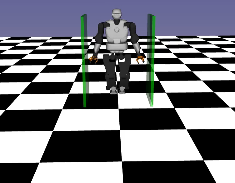
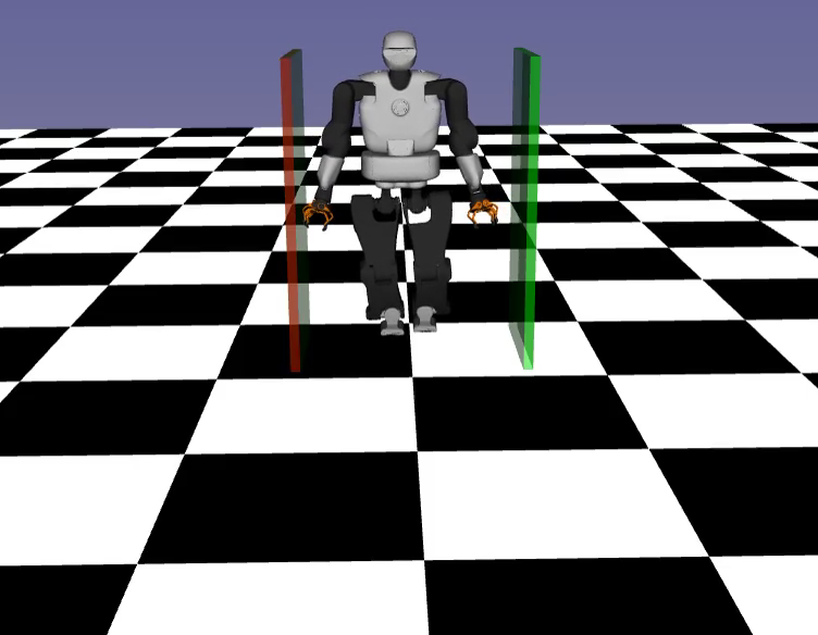
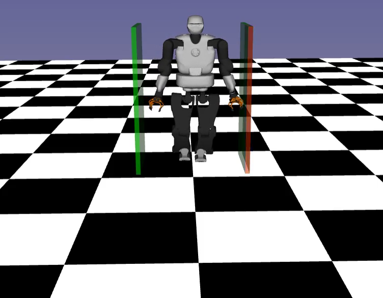
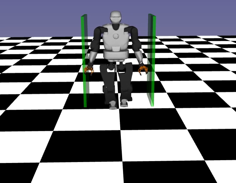
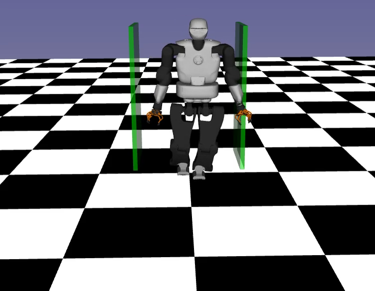
In this section, we present simulation results of the generated walking motions of a Talos robot [27] subject to additive persistent disturbances on the lateral CoM dynamics. We compare the motions generated using SMPC subject to state and control chance constraints against nominal MPC and tube-based RMPC. The lateral CoM position is constrained inside a box $-0.04\leq c^{y}\leq 0.04$ to avoid collision of the external parts of the robot with walls as it navigates through a narrow hallway with fixed contact locations as shown in Fig. 5. The CoM trajectories generated using MPC are tracked with a Task-Space Inverse Dynamics (TSID) controller using a hard contact model for generating the control commands [19]. We use the Pinocchio library  [28] for the computation of rigid-body dynamics. We show an empirical study comparing robustness w.r.t. performance of SMPC against tube-based RMPC and nominal MPC when subject to the same disturbance realizations. The robot model and simulation parameters are defined in Table I.

VI-A Hard constraints satisfaction in tube-based RMPC

First, we compute offline the state and control back-off magnitudes to tighten the constraint sets for RMPC.

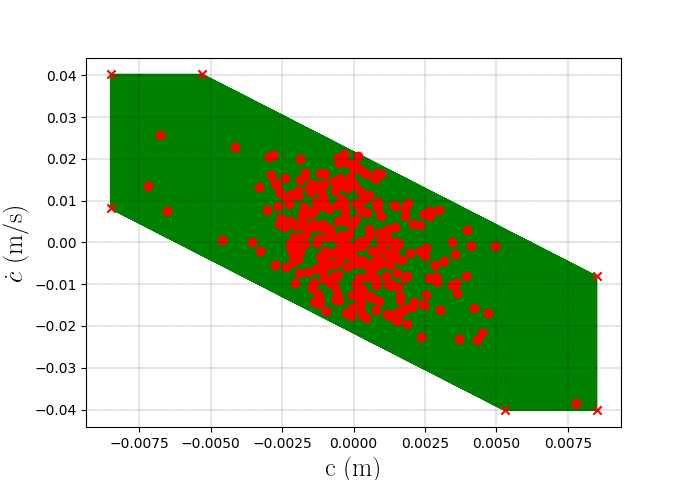
The state constraints back-off magnitude is computed using an outer $\epsilon$ approximation of the mRPI set $\Omega$ using the procedure in [23], with an accuracy of $\epsilon=10^{-6}$. In Fig. 1, we test the positive invariance property (1) of $\Omega$, by simulating $6$ initial conditions starting at the set vertices for $50$ time steps, and applying randomly sampled disturbance realizations from the disturbance set $\mathcal{W}$. As shown, the evolution of each initial condition (red dots), is kept inside $\Omega$ (the tube section) when subject to disturbance realizations $w_{t+i}\in\mathcal{W}=\begin{bmatrix}\mathcal{W}_{c}&\mathcal{W}_{\dot{c}}\end{bmatrix}^{\top}$. Using the same choice of pre-stabilizing dead-beat gains $K=\begin{bmatrix}3.386&0.968\end{bmatrix}$ as in [12], the robust control back-off magnitude $K\Omega$ is computed exactly without resorting to numerical approximation $K\Omega=K\mathcal{W}=\begin{bmatrix}-0.0225,&0.0225\end{bmatrix}$.

Figure 1: Simulation of $6$ initial conditions (red crosses) at the vertices of the outer-$\epsilon$ approximation of the mRPI set $\Omega$ for $50$ time steps subject to $w_{t+i}\in\mathcal{W}$.

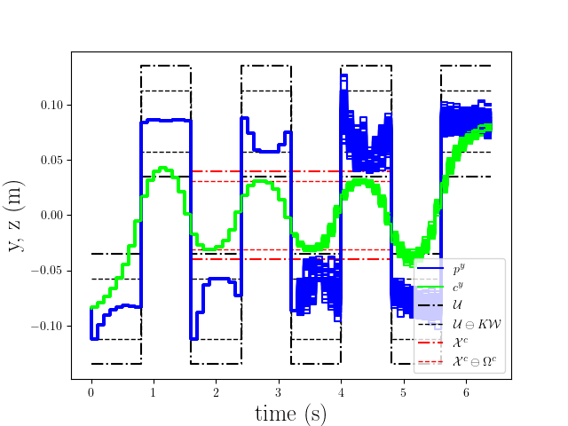
In Fig. 2, we plot the CoM position and CoP of $200$ trajectories obtained using tube-based RMPC. The robot takes the first two steps in place before entering the hallway. In the third and fourth steps, no disturbances were applied showing that the CoM position $c$ trajectories back off conservatively from the constraint bounds with the magnitude of the mRPI set on the CoM position $\Omega_{c}$. Finally, we randomly apply sampled Gaussian disturbance realizations $w_{t+i}\sim\mathcal{N}(0,\Sigma_{w})$ with finite support $\mathcal{W}$, where $\Sigma_{w}=\left[\begin{smallmatrix}\sigma^{2}_{c}&0\\ 0&\sigma^{2}_{\dot{c}}\end{smallmatrix}\right]$, for the rest of the motion, showing that both state and control constraints are satisfied as expected. Note that when the worst-case disturbance is persistently applied on one direction, the state constraint is saturated in that direction as expected. This shows that tube-based RMPC anticipates for a persistent worst-case disturbance to guarantee a hard constraint satisfaction, which is quite conservative and sub-optimal when the nature of the disturbances is stochastic as in this scenario.

VI-B Chance-constraints satisfaction in SMPC

This subsection presents the results of SMPC. Contrary to RMPC, the state and control back-off magnitudes ($\eta_{x_{t+i+1|t}}$, $\eta_{u_{t+i}}$) vary along the horizon, and are computed based on the propagation of the predicted state covariance (34), pre-stabilizing feedback gain $K$, disturbance covariance $\Sigma_{w}$, and the desired probability level of individual state and control constraint violation $\beta_{x_{j}}$ and $\beta_{u_{j}}$ respectively. We set $\beta_{x_{j}}=5\%$ , and $\beta_{u_{j}}=50\%$, which corresponds to satisfying the nominal CoP constraints.

Figure 2: 200 simulations of tube-based RMPC with $w_{t+i}\in\mathcal{W}$.

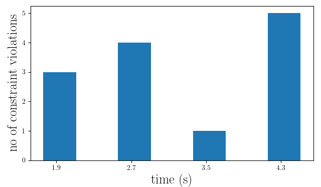
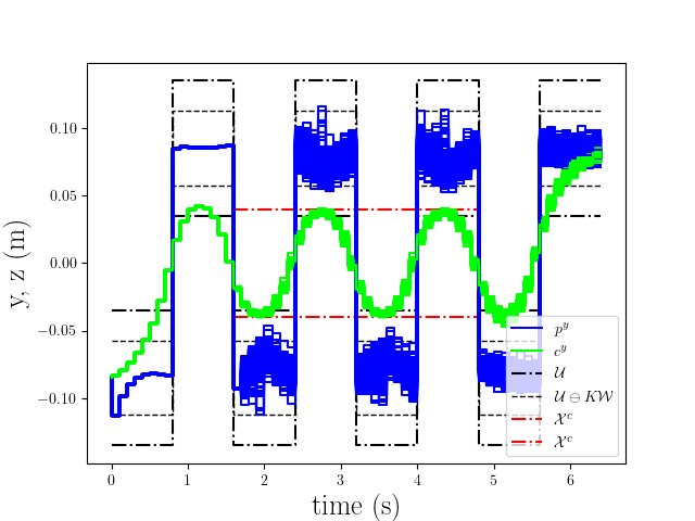
Using the same choice of stabilizing feedback gains $K$ as in RMPC, we simulate $200$ trajectories using SMPC in Fig. 3(b). In the first two steps, the robot steps in place and the CoM constraints are not active. For the rest of the motion, we randomly apply sampled Gaussian disturbance realizations $w_{t+i}\sim\mathcal{N}(0,\Sigma_{w})$ with finite support $\mathcal{W}$. In Fig. 3(a), we show the empirical number of CoM position constraint violations out of the $200$ simulated trajectories. The maximum number of constraint violations is obtained at time instance $4.3$s is $5(\leq 10$), which respects the designed probability level of CoM constraint violations $\beta_{x_{j}}=5\%$ as expected.

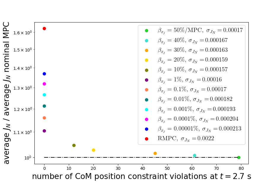
To test robustness of constraint satisfaction and optimality of SMPC, we ran an empirical study of the same eight step walking motion ($200$ trajectories) comparing SMPC with varying $\beta_{x_{j}}\in\begin{bmatrix}$0.00001\%$,&50\%\end{bmatrix}$ and fixed $\beta_{u_{j}}=50\%$ against tube-based RMPC and nominal MPC in Fig. 4. We plot the empirical number of CoM position constraint violations at $t=2.7$s, against the averaged cost performance (of $200$ trajectories) ratio between different MPC schemes and nominal MPC. As before, disturbance realizations are sampled from $\mathcal{N}(0,\Sigma_{w})$ with finite support $\mathcal{W}$. As expected, the higher the probability level of constraint satisfaction in SMPC, the lower the amount of constraint violations (higher robustness). The highest number of constraint violations is obtained at $\beta_{x_{j}}=50\%$, which is equivalent to nominal MPC. Zero constraint violations were obtained when $\beta_{x_{j}}\leq 1\%$, as for RMPC. An advantage of SMPC with $\beta_{x_{j}}\leq 1\%$ over RMPC, is the lower average cost. This gives the user the flexibility to design the controller for different task constraints, by tuning the probability level of constraint satisfaction without sacrificing performance as in tube-based RMPC or sacrificing robustness as in nominal MPC.

VII Discussion and Conclusions

This paper compared the use of SMPC with RMPC to account for uncertainties in bipedal locomotion. Many SMPC and RMPC algorithms exist. We decided to focus on two particular instances of tube-based approaches, which have the same online computational complexity as nominal MPC. Indeed, all the extra computation takes place offline, and consists in the design of tightened constraints (back-offs) based on a fixed pre-stabilizing feedback gain $K$.

(a) CoM position constraint violations.

(b) CoP and CoM lateral motion with $\beta_{x_{j}}=\,5\%$, $\beta_{u_{j}}=\,50\%$.

Figure 3: $200$ SMPC simulations with $w_{t+i}\sim\mathcal{N}(0,\Sigma_{w})\in\mathcal{W}$.

Our comparison focused on the trade off between robustness and optimality. Our tests show that, while SMPC does not provide hard guarantees on constraint satisfaction, in practice we did not observe any constraint violation with sufficiently low $\beta_{x}(\leq 1\%)$. This comes with the advantage of less conservative control, i.e. it results in better performance as measured by the cost function. This is reasonable because RMPC behaves conservatively, expecting a persistent worst-case disturbance, which in practice is extremely unlikely to happen. SMPC instead reasons about the probability of disturbances. In Section (V) we showed that we can compute the maximum disturbance sets to which SMPC ensures robustness. We showed that these sets shrink contractively as time grows. Loosely speaking, SMPC can be thought as a special kind of RMPC that considers shrinking disturbance sets along the horizon.

Our empirical results are specific to the choice of dead-beat feedback gains used in both algorithms. These gains were computed in [12] by minimizing the back-off magnitude on the CoP constraints. This is sensible because the CoP is usually more constrained than the CoM in bipedal locomotion. Other feedback gains could be used, such as LQR gains, resulting in back-off magnitudes that are a trade-off between state and control constraints.

Figure 4: SMPC with varying $\beta_{x_{j}}$ vs RMPC of $200$ simulations with $w_{t+i}\sim\mathcal{N}(0,\Sigma_{w})\in\mathcal{W}$. The dotted line denotes the optimal ratio of one (nominal MPC)

While changing the gains would affect our quantitative results, it would not affect the qualitative differences between SMPC and RMPC that we highlighted in the paper.

In conclusion, SMPC offers an opportunity for the control of walking robots that affords trading-off robustness to uncertainty and performance. For Future work, we intend to investigate nonlinear versions of RMPC and SMPC [29],[30] to enable the use of more complex models of locomotion.

Figure 5: TALOS robot walking through a narrow hallway using nominal MPC subject to additive disturbances on the lateral CoM dynamics. The Red color corresponds to the robot colliding with the wall.

-A Proof that $\alpha_{i}$ is monotonically decreasing (1D case):

We would like to show that $\alpha_{i+1}<\alpha_{i}\,,\,\,\forall i\geq 0$. Given

$$\alpha_{i}=\frac{\sum_{j=0}^{i}b^{2}_{j}\,\sigma^{2}_{w}}{(\sum_{j=0}^{i}|b_{j}|\sigma_{w})^{2}}\quad\alpha_{i+1}=\frac{\sum_{j=0}^{i+1}b^{2}_{j}\,\sigma^{2}_{w}}{(\sum_{j=0}^{i+1}|b_{j}|\sigma_{w})^{2}},$$ (51)

where $b_{j}=q^{\top}A_{K}^{j}$ can be written as $qa^{j}$, with $a\triangleq A_{K}$, $|a|<1$. After simplifying $\sigma_{w}$ we get:

(52)

By substituting the analytical expressions of the following series in (52)

$$\small\small\sum_{j=0}^{i}|b_{j}|=|q|\sum_{j=0}^{i}|a|^{j}=|q|\left(\frac{1-|a|^{i+1}}{1-|a|}\right),$$ (53a)

$$\sum_{j=0}^{i}b^{2}_{j}=q^{2}\sum_{j=0}^{i}a^{2j}=q^{2}\left(\frac{1-a^{2(i+1)}}{1-a^{2}}\right).$$ (54a)

and cross multiplication, we get

$$\small|q|^{3}\left(\frac{1-|a|^{i+1}}{1-|a|}\right)^{2}|a|^{i+1}\leq$$

$$q^{2}\left(\frac{1-a^{2(i+1)}}{1-a^{2}}\right)\left(|qa^{i+1}|+2|q|\left(\frac{1-|a|^{i+1}}{1-|a|}\right)\right).$$ (55)

By multiplying both sides of (-A) by $\frac{(1-|a|)^{2}}{|q|^{3}}$, we have

$$\small|a|^{i+1}(1-|a|^{i+1})^{2}\leq\frac{1-a^{2(i+1)}}{1+a}\left(|a|^{i+1}(1-|a|)+2(1-|a|^{i+1})\right)$$

$$\Rightarrow(1+|a|)(|a|^{i+1}-a^{2i+2})\leq(1+|a|^{i+1})(-|a|^{i+1}-|a|^{i+2}+2)$$

$$\Rightarrow|a|^{i+1}+|a|^{i+2}-|a|^{2i+3}\leq 2+|a|^{i+1}-|a|^{i+2}-|a|^{2i+3}$$

$$\Rightarrow 2-2|a|^{i+2}\geq 0,$$ (56)

which always holds because $|a|<1$. This concludes the proof. ∎

References

- [1] D. Mayne, J. Rawlings, C. Rao, and P. Scokaert, “Constrained model predictive control: Stability and optimality,” Automatica, vol. 36, no. 6, pp. 789 – 814, 2000.
- [2] J. Rawlings, D. Mayne, and M. Diehl, Model Predictive Control: Theory, Computation, and Design, 01 2017.
- [3] P. Wieber, “Trajectory free linear model predictive control for stable walking in the presence of strong perturbations,” pp. 137–142, 2006.
- [4] A. Herdt, H. Diedam, P.-B. Wieber, D. Dimitrov, K. Mombaur, and M. Diehl, “Online walking motion generation with automatic foot step placement,” Advanced Robotics, vol. 24, pp. 719–737, 04 2010.
- [5] A. Sherikov, D. Dimitrov, and P.-B. Wieber, “Whole body motion controller with long-term balance constraints,” in 2014 IEEE-RAS International Conference on Humanoid Robots. IEEE, 2014, pp. 444–450.
- [6] C. Brasseur, A. Sherikov, C. Collette, D. Dimitrov, and P.-B. Wieber, “A robust linear mpc approach to online generation of 3d biped walking motion,” in 2015 IEEE-RAS 15th International Conference on Humanoid Robots (Humanoids). IEEE, 2015, pp. 595–601.
- [7] H. Dai and R. Tedrake, “Planning robust walking motion on uneven terrain via convex optimization,” in 2016 IEEE-RAS 16th International Conference on Humanoid Robots (Humanoids). IEEE, 2016, pp. 579–586.
- [8] N. Bohórquez and P.-B. Wieber, “Adaptive step duration in biped walking: a robust approach to nonlinear constraints,” in 2017 IEEE-RAS 17th International Conference on Humanoid Robotics (Humanoids). IEEE, 2017, pp. 724–729.
- [9] D. Q. Mayne and W. Langson, “Robustifying model predictive control of constrained linear systems,” Electronics Letters, vol. 37, no. 23, pp. 1422–1423, 2001.
- [10] L. Chisci, J. Rossiter, and G. Zappa, “Systems with persistent disturbances: predictive control with restricted constraints,” Automatica, vol. 37, no. 7, pp. 1019 – 1028, 2001.
- [11] D. Mayne, M. Seron, and S. Raković, “Robust model predictive control of constrained linear systems with bounded disturbances,” Automatica, vol. 41, no. 2, pp. 219 – 224, 2005.
- [12] N. A. Villa and P. Wieber, “Model predictive control of biped walking with bounded uncertainties,” in 2017 IEEE-RAS 17th International Conference on Humanoid Robotics (Humanoids), 2017, pp. 836–841.
- [13] M. Cannon, “Model predictive control,” University of Oxford, Hilary Term, 2016.
- [14] T. A. N. Heirung, J. A. Paulson, J. O’Leary, and A. Mesbah, “Stochastic model predictive control — how does it work?” Computers & Chemical Engineering, vol. 114, pp. 158 – 170, 2018, fOCAPO/CPC 2017.
- [15] M. Farina, L. Giulioni, and R. Scattolini, “Stochastic linear model predictive control with chance constraints – a review,” Journal of Process Control, vol. 44, pp. 53 – 67, 2016.
- [16] M. Lorenzen, F. Dabbene, R. Tempo, and F. Allgöwer, “Constraint-tightening and stability in stochastic model predictive control,” IEEE Transactions on Automatic Control, vol. 62, no. 7, pp. 3165–3177, July 2017.
- [17] M. Ciocca, P.-B. Wieber, and T. Fraichard, “Effect of planning period on mpc-based navigation for a biped robot in a crowd,” 2019.
- [18] G. Wiedebach, S. Bertrand, T. Wu, L. Fiorio, S. McCrory, R. Griffin, F. Nori, and J. Pratt, “Walking on partial footholds including line contacts with the humanoid robot atlas,” in 2016 IEEE-RAS 16th International Conference on Humanoid Robots (Humanoids). IEEE, 2016, pp. 1312–1319.
- [19] A. Del Prete and N. Mansard, “Robustness to joint-torque-tracking errors in task-space inverse dynamics,” IEEE transactions on Robotics, vol. 32, no. 5, pp. 1091–1105, 2016.
- [20] P.-B. Wieber, R. Tedrake, and S. Kuindersma, Modeling and Control of Legged Robots, 2016, pp. 1203–1234.
- [21] T. Koolen, T. De Boer, J. Rebula, A. Goswami, and J. Pratt, “Capturability-based analysis and control of legged locomotion, part 1: Theory and application to three simple gait models,” The international journal of robotics research, vol. 31, no. 9, pp. 1094–1113, 2012.
- [22] F. Blanchini and S. Miani, Set-theoretic methods in control. Springer, 2008.
- [23] S. V. Rakovic, E. C. Kerrigan, K. I. Kouramas, and D. Q. Mayne, “Invariant approximations of the minimal robust positively invariant set,” IEEE Transactions on Automatic Control, vol. 50, no. 3, pp. 406–410, March 2005.
- [24] L. Hewing and M. N. Zeilinger, “Stochastic model predictive control for linear systems using probabilistic reachable sets,” in 2018 IEEE Conference on Decision and Control (CDC). IEEE, 2018, pp. 5182–5188.
- [25] D. Mayne, “Robust and stochastic mpc: Are we going in the right direction?” IFAC-PapersOnLine, vol. 48, no. 23, pp. 1 – 8, 2015, 5th IFAC Conference on Nonlinear Model Predictive Control NMPC 2015.
- [26] J. Paulson, T. Santos, and A. Mesbah, “Mixed stochastic-deterministic tube mpc for offset-free tracking in the presence of plant-model mismatch,” Journal of Process Control, vol. 83, pp. 102 – 120, 2019.
- [27] O. Stasse, T. Flayols, R. Budhiraja, K. Giraud-Esclasse, J. Carpentier, J. Mirabel, A. Del Prete, P. Soueres, N. Mansard, F. Lamiraux, J.-P. Laumond, L. Marchionni, H. Tome, and F. Ferro, “TALOS: A new humanoid research platform targeted for industrial applications,” in IEEE-RAS International Conference on Humanoid Robots, vol. Part F1341, 2017.
- [28] J. Carpentier, G. Saurel, G. Buondonno, J. Mirabel, F. Lamiraux, O. Stasse, and N. Mansard, “The pinocchio c++ library – a fast and flexible implementation of rigid body dynamics algorithms and their analytical derivatives,” in IEEE International Symposium on System Integrations (SII), 2019.
- [29] J. Köehler, M. A. Müller, and F. Allgöwer, “A nonlinear model predictive control framework using reference generic terminal ingredients,” IEEE Transactions on Automatic Control, pp. 1–1, 2019.
- [30] T. L. M. Santos, A. D. Bonzanini, T. A. N. Heirung, and A. Mesbah, “A constraint-tightening approach to nonlinear model predictive control with chance constraints for stochastic systems,” in 2019 American Control Conference (ACC), 2019, pp. 1641–1647.