Fireshape: a shape optimization toolbox for Firedrake

Abstract

We introduce Fireshape, an open-source and automated shape optimization toolbox for the finite element software Firedrake. Fireshape is based on the moving mesh method and allows users with minimal shape optimization knowledge to tackle with ease challenging shape optimization problems constrained to partial differential equations (PDEs).

1 Introduction

One of the ultimate goals of structural optimization is the development of fully automated software that allows users to tackle challenging structural optimization problems in the automotive, naval, and aerospace industries without requiring deep knowledge of structural optimization theory. The scientific community is working actively in this direction, and recent years have seen the publication of educational material that simplifies the understanding of structural optimization algorithms and guides the development of related optimization software. These resources are based on different models, such as moving mesh methods AlPa06 ; DaFrOm18 ; CoLePrFrLa19 ; Al07 , level-sets La18 ; AlJoTo02 ; BeWaBe19 , phase fields GaHeHiKa15 ; DoPoRuSi20 ; BlGaFaHaSt14 , and SIMP Si01 ; polytop12 ; Be89 ; BeSi04 , and are implemented in various software environments such as Matlab Si01 ; polytop12 , FreeFem++ AlPa06 ; DaFrOm18 ; AlJoTo02 , OpenFOAM CFD CoLePrFrLa19 , FEMLAB LiKoHu05 , and FEniCS La18 ; DoFuJoSc19 , to mention just a few.

In this work, we introduce Fireshape: an automated shape optimization library based on the moving mesh approach that requires very limited input from the user. Shape optimization refers to the optimization of domain boundaries and plays an important role in structural design. For instance, shape optimization plays a crucial role in the design of airfoils HeJiMaYiMa19 ; WaDoJi18 ; ScIlScGa13 and boat hulls LoPaQuRo12 ; MaVuCu16 ; AbSu17 . Shape optimization is also a useful refinement step to be employed after topology optimization (BeSi04, , Ch. 1.4). Indeed, topology optimization allows more flexibility in geometric changes and it is a powerful tool to explore a large design space. However, topology optimization may return slightly blurred (grey-scale) and/or staircase designs BeSi04 . By adding a final shape optimization step, it is possible to post-process results computed with topology optimization and devise optimal designs with sharp boundaries and interfaces, when this is necessary.

Fireshape is based on the moving mesh shape optimization approach (Al07, , Ch. 6). In this approach, geometries are parametrized with meshes that can be arbitrarily precise and possibly curvilinear. The mesh nodes and faces are then optimized (or “moved”) to minimize a chosen target function. Fireshape has been developed on the moving mesh approach because the latter has a very neat interpretation in terms of geometric transformations and is inherently compatible with standard finite element software, as it relies on the canonical construction of finite elements via pullbacks PaWeFa18 . The main drawback of the moving mesh approach is that it does not allow topological changes in a straightforward and consistent fashion. However, Fireshape has been developed to facilitate shape optimization, and topology optimization is beyond its scope.

Fireshape couples the finite element library Firedrake Firedrake1 ; Firedrake2 ; Firedrake3 ; Firedrake4 ; Firedrake5 with the Rapid Optimization Library (ROL) ROL . Fireshape allows decoupled discretization of geometries and state constraints and it includes all necessary routines to perform shape optimization (geometry updates, regularization terms, geometric constraints, etc.). To solve a shape optimization problem in Fireshape, users must describe the objective function and the eventual constraints using the Unified Form Language (UFL) AlLoOlRoWe14 , a language embedded in Python to describe variational forms and their finite element discretizations that is very similar to standard mathematical notation. Once objective functions and constraints have been implemented with UFL, users need only to provide a mesh that describes the initial design and, finally, select their favorite optimization algorithm from the optimization library ROL, which contains algorithms for unconstrained, bound constrained, and (in-)equality constrained optimisation problems. In particular, users do not need to spend time deriving shape derivative formulas and adjoint equations by hand, nor worry about their discretization, because Fireshape automates these tasks.

Typically the computational bottleneck of PDE constrained optimization code lies in the solution of the state and the adjoint equation. While Fireshape and Firedrake are both written in Python, to assemble the state and adjoint equations the Firedrake library automatically generates optimized kernels in the C programming language. The generated systems of equations are then passed to the PETSc library (also written in C) and can be solved using any of the many linear solvers and preconditioners accessible from PETSc petsc1 ; petsc2 ; petsc3 ; petsc4 ; petsc5 ; petsc6 . This combination of Python for user facing code and C for performance critical parts is well established in scientific computing as it provides highly performant code that is straightforward to develop and use. Finally, we mention that Fireshape, just as Firedrake, PETSc and ROL, supports MPI parallelization and hence can be used to solve even large scale three dimensional shape optimization problems. In particular, Firedrake has been used to solve systems with several billion degrees of freedom on supercomputers with tens of thousands of cores (see e.g. mitchell_high_2016 ; farrell2019augmented ), and we emphasize that any PDE solver written in Firedrake can be used for shape optimization problems with Fireshape.

Fireshape is an open-source software licensed under the GNU Lesser General Public License v3.0. Fireshape can be downloaded at

https://github.com/Fireshape/Fireshape .

Its documentation contains several tutorials and is available at

https://fireshape.readthedocs.io/en/latest/ .

To illustrate Fireshape’s capabilities and ease of use, in Section 2 we provide a tutorial and solve a three-dimensional shape optimization problem constrained by the nonlinear Navier-Stokes equations. The shape optimization knowledge required to understand this tutorial is minimal. In Section 3, we provide another tutorial based on a shape optimization problem constrained to the linear elasticity equation. In Section 4, we describe in detail the rich mathematical theory that underpins Fireshape. In Section 5, we describe Fireshape’s main classes and Fireshape’s extended functionality. Finally, in Section 6, we provide concluding remarks.

2 Example: Shape optimization of a pipe

For this hands-on introduction to Fireshape, we first consider a viscous fluid flowing through a pipe $\rm{\Omega}$ (see Figure 1) and aim to minimize the kinetic energy dissipation into heat by optimizing the design of $\rm{\Omega}$. This is a standard test case ZhLi08 ; ViMa17 ; FeAlDaJo20 ; DiDiFuSiLa18 ; DaFaMiAl17 . To begin with, we need to describe this optimization problem with a mathematical model.

Figure 1: Viscous fluid flows through a pipe $\rm{\Omega}$ from the left to the right. A poor pipe design can lead to an excessive amount of kinetic energy being dissipated into heat.

We assume that the fluid velocity ${\mathbf{u}}$ and the fluid pressure $\rm p$ satisfy the incompressible Navier-Stokes equations (ElSiWa14, , Eqn. 8.1), which read

$$-2\nu\nabla\cdot\varepsilon{\mathbf{u}}+({\mathbf{u}}\cdot\nabla){\mathbf{u}}+\nabla\rm{p} =0 \text{in }\rm{\Omega}\,,$$ (1a)

$$\operatorname{div}{\mathbf{u}} =0 \text{in }\rm{\Omega}\,,$$ (1b)

$${\mathbf{u}} ={\mathbf{g}} \text{on }\partial\rm{\Omega}\setminus\rm{\Gamma}\,,$$ (1c)

$$\rm{p}{\mathbf{n}}-2\nu\varepsilon{\mathbf{u}}\,{\mathbf{n}} =0 \text{on }\rm{\Gamma}\,,$$ (1d)

where $\nu$ denotes the fluid viscosity, $\varepsilon{\mathbf{u}}=\varepsilon({\mathbf{u}})=\frac{1}{2}(\nabla{\mathbf{u}}+\nabla{\mathbf{u}}^{\top})$, $\nabla{\mathbf{u}}$ is the derivative (Jacobian matrix) of ${\mathbf{u}}$ and $\nabla{\mathbf{u}}^{\top}$ is the derivative transposed, $\rm{\Gamma}$ denotes the outlet, and the function ${\mathbf{g}}$ is a Poiseuille flow velocity (ElSiWa14, , p. 122) at the inlet and zero on the pipe walls. In our numerical experiment, the inlet is a disc of radius 0.5 in the xy-plane, and ${\mathbf{g}}(x,y,z)=(0,0,1-4(x^{2}+y^{2}))^{\top}$ on the inlet.

To model the kinetic energy dissipation, we consider the diffusion term in (1a) and introduce the function

$$\rm{J}(\rm{\Omega})=\int_{\rm{\Omega}}\nu\,\varepsilon{\mathbf{u}}:\varepsilon{\mathbf{u}}\,\mathrm{d}{\boldsymbol{x}}\,,$$ (2)

where the colon symbol $:$ denotes the Frobenius inner product, that is, $\varepsilon{\mathbf{u}}:\varepsilon{\mathbf{u}}=\rm{trace}((\varepsilon{\mathbf{u}})^{\top}\varepsilon{\mathbf{u}})$.

Now, we can formulate the shape optimizations problem we are considering. This reads:

$$\text{Find }{\rm\Omega}^{*}\text{ such that }\rm{J}(\rm{\Omega}^{*})=\inf\rm{J}(\rm{\Omega})\text{ subject to \eqref{eq:NavierStokes}.}$$ (3)

To make this test case more interesting, we further impose a volume equality constraint on $\rm{\Omega}$. Otherwise, without this volume constraint, the solution to this problem would be a pipe with arbitrarily large diameter.

In the next subsections, we explain step by step how to solve this shape optimization problem in Fireshape. To this end, we need to create: a mesh that approximates the initial guess $\rm\Omega$ (Section 2.1), an object that describes the PDE-constraint (1) (Section 2.2), an object that describes the objective function (2) (Section 2.3), and, finally, a “main file” to set up and solve the optimization problem (3) with the additional volume constraint (Section 2.4).

2.1 Step 1: Provide an initial guess

The first step is to provide a mesh that describes an initial guess of $\rm\Omega$. For this tutorial, we create this mesh using the software Gmsh GeRe09 . The initial guess employed is sketched in Figure 1. The only mesh detail necessary to understand this tutorial is that, in Listing 1, the number 10 corresponds to the inlet, wheres the boundary flags 12 and 13 refer to the pipe’s boundary. For the remaining geometric details, we refer to the code archived on Zenodo zenodo-firedrake-and-driver .

2.2 Step 2: Implement the PDE-constraint

The second step is to implement a finite element solver of the Navier-Stokes equations (1). To derive the weak formulation of (1a), we multiply Equation (1a) with a test (velocity) function ${\mathbf{v}}$ that vanishes on $\partial\rm{\Omega}\setminus\rm{\Gamma}$, and Equation (1b) with a test (pressure) function $\rm{q}$. Then, we integrate over $\rm\Omega$, integrate by parts (ElSiWa14, , Eq. 3.18), and impose the boundary condition (1d). The resulting weak formulation of equations (1) reads:

$$\text{Find }{\mathbf{u}}\text{ such that }{\mathbf{u}}={\mathbf{g}}\text{ on }\partial\rm\Omega\setminus\Gamma\text{ and}$$

$$\int_{\rm{\Omega}}2\nu\varepsilon{\mathbf{u}}:\varepsilon{\mathbf{v}}-\rm{p}\operatorname{div}({\mathbf{v}})+{\mathbf{v}}\cdot(\nabla{\mathbf{u}}){\mathbf{u}}+\rm{q}\operatorname{div}({\mathbf{u}})\,\mathrm{d}{\boldsymbol{x}}=0$$

$$\text{for any pair }({\mathbf{v}},\rm{q})\,.$$ (4)

List of mylistings 1 Incompressible Navier-Stokes solver based on Taylor-Hood finite elements.

To implement the finite element discretization of (2.2), we create a class NavierStokesSolver that inherits from the Fireshape’s class PdeConstraint, see Listing 1. To discretize (2.2), we employ P2-P1 Taylor-Hood finite elements, that is, we discretize the trial and test velocity functions ${\mathbf{u}}$ and ${\mathbf{v}}$ with piecewise quadratic Lagrangian finite elements, and the trial and test pressure functions $\rm{p}$ and $\rm{q}$ with piecewise affine Lagrangian finite elements. It is well known that this is a stable discretization of the incompressible Navier-Stokes equations (ElSiWa14, , pp 136-137).

To address the nonlinearity in (2.2), we use PETSc’s Scalable Nonlinear Equations Solvers (SNES) petsc1 ; petsc2 ; petsc3 ; petsc4 ; petsc5 ; petsc6 . In each iteration, SNES linearizes Equation (2.2) and solves the resulting system with a direct solver. In general, it is possible that the SNES solver fails to converge sufficiently quickly (in our code, we allow at most 100 SNES iterations). For instance, this happens if the finite element mesh self-intersects, or if the initial guess used to solve (2.2) is not sufficiently good. Most often, these situations happen when the optimization algorithm takes an optimization step that is too large. In these cases, we can address SNES’ failure to solve (2.2) by reducing the optimization step. In practice, we deal with these situations with Python’s try: ... except: ... block. If the SNES solver fails with a ConvergenceError, we catch this error and set the boolean flag self.failed_to_solve to True. This flag is used to adjust the output of the objective function $\rm{J}$, see Section 2.3.

2.3 Step 3: Implement the objective function

The third step is to implement a code to evaluate the objective function $\rm{J}$ defined in Equation (2). For this, we create a class EnergyDissipation that inherits from Fireshape’s class ShapeObjective, see Listing 2. Of course, evaluating $\rm{J}$ requires access to the fluid velocity ${\mathbf{u}}$. This access is implemented by assigning the variable self.pde_solver. This variable gives access also to the variable NavierStokesSolver.failed_to_solve, which can be used to control the output of $\rm{J}$ when the Navier-Stokes’ solver fails to converge. Here, we decide that the value of $\rm{J}$ is NaN (“not a number”) if the Navier-Stokes’ solver fails to converge.

List of mylistings 2 Objective function $\rm J$ (2), which quantifies the kinetic energy dissipation of the fluid. Note that $\rm J$ returns NaN (“not a number”) if the solver of the PDE-constraint (2.2) fails to converge.

2.4 Final step: Set up and solve the problem

At this stage, we have all the necessary ingredients to tackle the shape optimization problem (3). The final step is to create a “main file” that loads the initial mesh, sets-up the optimization problem, and solves it with an optimization algorithm. The rest of this section contains a line-by-line description of the “main file”, which is listed in Listing 3.

List of mylistings 3 Minimize the kinetic energy dissipation of a fluid using Fireshape.

• In lines 1-6, we import all necessary Python libraries and modules.

• In lines 8-13, we load the mesh of the initial design and we specify to discretize perturbations of the domain $\rm\Omega$ using quadratic B-splines with support in a box that does not include the inlet and the outlet. In this example, we also impose some boundary regularity on B-splines and limit perturbations to be only in direction of the $y$-axis. Sections 5.1 and 5.2 provide more details about the Fireshape classes ControlSpace and InnerProduct.

• In lines 15-16, we initiate the Navier-Stokes finite element solver.

• In lines 18-19, we tell Fireshape to store the finite element solution to Navier-Stokes’ equations in the folder solution every time the domain $\rm\Omega$ is updated. We can visualize the evolution of ${\mathbf{u}}$ along the optimization process by opening the file u.pvd with Paraview ahrens2005paraview .

• In lines 21-22, we initiate the objective function $\rm J$ and the associated reduced functional, which is used by Fireshape to define the appropriate Lagrange functionals to shape differentiate $\rm J$. We refer to Section 4.2 for more details about shape differentiation using Lagrangians. We stress that Fireshape does not require users to derive (and implement) shape derivative formulas by hand. The whole shape differentiation process is automated using pyadjoint HaMiPaWe19 ; DoMiFu20 , see Remark 1.

• In lines 24-25, we add an additional regularization term to $\rm J$ to promote mesh quality of domain updates. This regularization term controls the pointwise maximum singular value of the geometric transformation used to update $\rm\Omega$ wechsungthesis . See Section 4.2, Figure 9, and Remark 3 for more information about the role of geometric transformations in Fireshape.

• In lines 27-30, we set up an equality constraint to ensure that the volume of the initial and the optimized domains are equal.

• In lines 32-43, we select an optimization algorithm from the optimization library ROL. More specifically, we use an augmented Lagrangian approach (NoWr06, , Ch. 17.3) with limited-memory BFGS Hessian updates (NoWr06, , Ch. 6.1) to deal with the volume equality constraint, and a Trust-Region algorithm (NoWr06, , Ch. 4.1) to solve the intermediate models generated by the augmented Lagrangian algorithm.

• In lines 44-47, finally, we gather all information and solve the problem.

Remark 1

A reader may wonder why Fireshape does not require information about shape derivative formulas and adjoint equations to solve a PDE-constrained shape optimization problem. This is possible because Fireshape employs UFL’s and pyadjoint’s automated shape differentiation and adjoint derivation capabilities HaMiPaWe19 ; DoMiFu20 . In particular, UFL combines the automated construction of finite element pullbacks with symbolic differentiation to automate the evaluation of directional shape derivatives along vector fields discretized by finite elements HaMiPaWe19 . This process mimics the analytical differentiation of shape functions and is equivalent to the “optimize-then-discretize” paradigm, i.e. it yields exact (up to floating point accuracy) derivatives.

2.5 Results

Running the code contained in Listing 3 optimizes the pipe design when the fluid viscosity $\nu$ is 0.1, which corresponds to Reynold-number $\operatorname{Re}=1./\nu=10$. Of course, the resulting shape depends on the fluid viscosity. A natural question is how the optimized shape depends on this parameter. To answer this question, we can simply run Listing 3 for different Reynold-numbers (by modifying line 13 with the desired value) and inspect the results. Here we perform this comparison for $\operatorname{Re}\in\{1,250,500,750,1000\}$.

In Figure 2, we show the initial design and plot the magnitude of the fluid velocity on a cross section of the pipe for different Reynold-numbers.

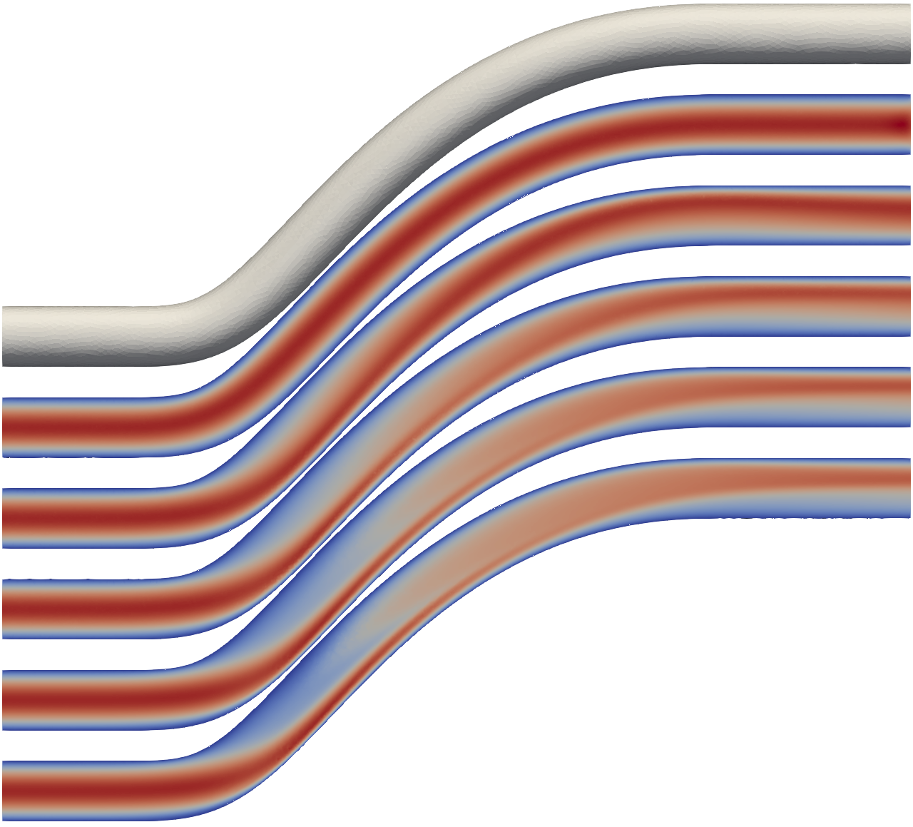
Figure 2: Initial design of the pipe and velocity solutions for $\operatorname{Re}=1,250,500,750,1000$ (from top to bottom) inside the pipe. Red corresponds to high velocity, blue corresponds to low velocity.

In Figure 3, we show the resulting optimized shapes, and in Figure 4 the corresponding magnitudes of the fluid velocity. Qualitatively, we observe that, as the Reynolds-number increase, we obtain increasingly S-shaped designs that avoid high curvature at the two fixed ends. Finally, we remark that the objective is reduced by approximately $6.9\%$, $9.5\%$, $10.8\%$, $11.7\%$ and $12.1\%$ in at most 10 augmented Lagrangian steps, respectively. Each numerical experiment was run in parallel on a server with 36 cores.

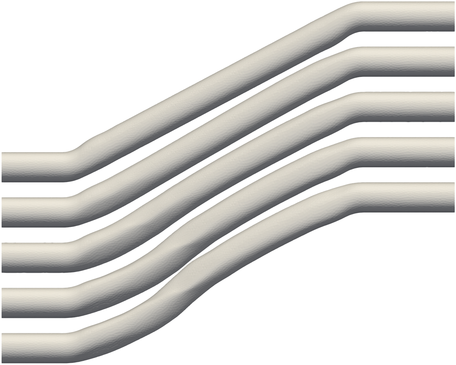
Figure 3: Optimized shapes for $\operatorname{Re}=1,250,500,750,1000$ (from top to bottom).

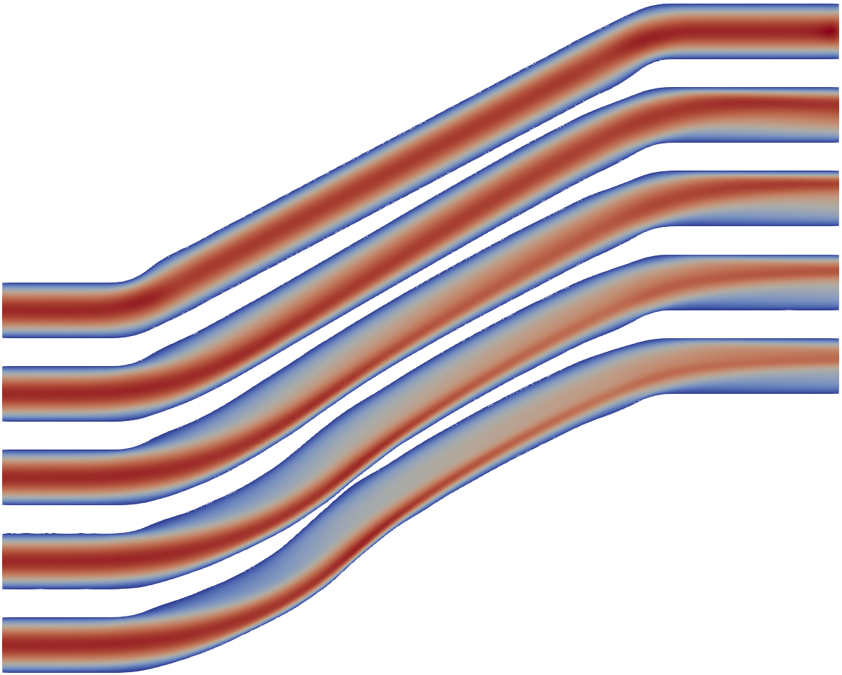
Figure 4: Velocity field for optimized shapes for $\operatorname{Re}=1,250,500,750,1000$ (from top to bottom). Red corresponds to high velocity, blue corresponds to low velocity.

3 Example: Shape optimization of a cantilever

In this second tutorial, we consider another shape optimization classic AlPa06 ; Al07 : the minimization of the compliance of a cantilever $\rm{\Omega}$ (see Figure 5) subject to a dead surface load ${\mathbf{g}}$. To make this example reproducible on a basic laptop we consider a two dimensional version of this problem. Adapting the code presented in this section to simulate a three dimensional cantilever is straightforward.

Figure 5: A cantilever is attached to a wall on the left ($\Gamma_{1}$) and pulled downwards on the right ($\Gamma_{2}$) by a dead surface load. A poor cantilever design may fail to offer sufficient support.

We model the cantilever elastic response using the linear elasticity equations (Br07, , Ch. VI, Sect. 3). More precisely, we consider the displacement formulation: the displacement field ${\mathbf{u}}$ satisfies the variational problem

$$\int_{\rm\Omega}\sigma({\mathbf{u}}):\epsilon({\mathbf{v}})\,\mathrm{d}{\boldsymbol{x}}=\int_{\Gamma_{2}}{\mathbf{g}}\cdot{\mathbf{v}}\,\mathrm{d}S\quad\text{ for every }{\mathbf{v}}\,,$$ (5)

where $\sigma({\mathbf{u}})=\lambda\operatorname{div}({\mathbf{u}})\rm{I}+2\mu\varepsilon({\mathbf{u}})$, $\lambda$ and $\mu$ are the Lamé constants, $\rm{I}$ is the identity matrix, $\varepsilon({\mathbf{u}})=\frac{1}{2}(\nabla{\mathbf{u}}+\nabla{\mathbf{u}}^{\top})$, $\nabla{\mathbf{u}}$ is the derivative (Jacobian matrix) of ${\mathbf{u}}$ and $\nabla{\mathbf{u}}^{\top}$ is the derivative transposed, the colon symbol $:$ denotes the Frobenius inner product, that is $\sigma(u):\varepsilon({\mathbf{v}})=trace(\sigma({\mathbf{u}})^{\top}\varepsilon({\mathbf{v}}))$, and $\Gamma_{2}$ denotes the part of the boundary that is subject to the surface load ${\mathbf{g}}$. Additionally, although not explicitly indicated in (5), the displacement ${\mathbf{u}}$ vanishes on $\Gamma_{1}$, which is the part of the boundary $\partial\rm\Omega$ that corresponds to the wall, see Figure 5.

To model the compliance of the structure $\rm\Omega$, we consider the functional

$$\rm{J}(\rm{\Omega})=\int_{\rm{\Omega}}\sigma({\mathbf{u}}):\varepsilon({\mathbf{u}})\,\mathrm{d}{\boldsymbol{x}}\,,$$ (6)

where ${\mathbf{u}}$ is the displacement and satisfies (5).

As typical for this shape optimization test case, we also impose a volume equality constraint on $\rm\Omega$ to prescribe the amount of material used to fabricate the cantilever.

Similarly to Section 2, in the following subsections we explain how to solve this shape optimization test case in Fireshape.

3.1 Step 1: Provide an initial guess

To create the mesh of the initial guess, we use again the software Gmsh GeRe09 . The initial guess employed is sketched in Figure 5. The only mesh detail necessary to understand this tutorial is that, in Listing 4, the number 1 corresponds to $\Gamma_{1}$, whereas the boundary flag 2 refers to $\Gamma_{2}$. For the remaining geometric details, we refer to the code archived on Zenodo zenodo-firedrake-and-driver .

3.2 Step 2: Implement the PDE-constraint

In this example, the PDE constraint (5) is already in weak form. To implement its finite element discretization, we create a class LinearElasticitySolver that inherits from Fireshape’s class PdeConstraint, see Listing 4. To discretize (5), we employ the standard piecewise affine Lagrangian finite elements (Br07, , Ch. II, Sect. 5). To solve the resulting linear system, we employ a direct solver. This is sufficiently fast for the current 2D example. For readers interested in creating a three dimensional version of this example, we suggest replacing the direct solver with a Krylov method preconditioned by one of the algebraic multigrid methods that can be accessed via PETSc.

List of mylistings 4 Linear elasticity solver.

3.3 Step 3: Implement the objective function

We implement the objective function $\rm{J}$ defined in Equation (6) in a class Compliance that inherits from Fireshape’s class ShapeObjective, see Listing 5. This functional accesses the displacement field ${\mathbf{u}}$ via the variable self.pde_solver.

To verify that the domain used to compute ${\mathbf{u}}$ is feasible, that is, that the mesh is not tangled, we create a piecewise constant function detDT and interpolate the determinant of the derivative of the transformation ${\mathbf{T}}$ used to generated the updated domains (see Section 4.2 and 4.3 for more details about the role of the transformation ${\mathbf{T}}$ in Fireshape). If the minimum of detDT is a small number, this indicates that the mesh has poor quality (see also Remark 3), and this negatively affects the accuracy of the finite element method. In this case, we decide that the value of $\rm{J}$ is NaN (“not a number”) to ensure that only trustworthy simulations are used .

List of mylistings 5 Objective function $\rm J$ (6), which quantifies the compliance of the structure. Note that $\rm J$ returns NaN (“not a number”) if the mesh has poor quality.

3.4 Final step: Set up and solve the problem

Finally, to shape optimize the initial desing we create a “main file” that loads the initial mesh, sets-up the optimization problem, and solves it with an optimization algorithm. The rest of this section contains a line-by-line description of the “main file”, which is listed in Listing 6.

List of mylistings 6 Minimize the kinetic energy dissipation of a fluid using Fireshape.

• In lines 1-6, we import all necessary Python libraries and modules.

• In lines 8-11, we load the mesh of the initial design and we specify to discretize perturbations of the domain $\rm\Omega$ using piecewise affine Lagrangian finite elements. We also employ a metric inspired by the linear elasticity equations and specify that the boundaries $\Gamma_{1}$ and $\Gamma_{2}$ cannot be modified. Sections 5.1 and 5.2 provide more details about the Fireshape classes ControlSpace and InnerProduct.

• In line 13, we initiate the linear elasticity solver.

• In lines 15-16, we tell Fireshape to store the finite element approximation of the displacement field ${\mathbf{u}}$ in the folder solution every time the domain $\rm\Omega$ is updated. We can visualize the evolution of ${\mathbf{u}}$ along the optimization process by opening the file u.pvd with Paraview ahrens2005paraview .

• In lines 18-19, we initiate the objective function $\rm J$ and the associated reduced functional, which is used by Fireshape to define the appropriate Lagrange functionals to shape differentiate $\rm J$. We refer to Section 4.2 for more details about shape differentiation using Lagrangians. Note that, as mentioned in Remark 1, Fireshape does not require users to derive (and implement) shape derivative formulas by hand. The whole shape differentiation process is automated using pyadjoint HaMiPaWe19 ; DoMiFu20 .

• In lines 21-22, we add an additional regularization term to $\rm J$ to promote mesh quality of domain updates. This regularization term controls the pointwise maximum singular value of the geometric transformation used to update $\rm\Omega$ wechsungthesis . See Section 4.2, Figure 9, and Remark 3 for more information about the role of geometric transformations in Fireshape.

• In lines 24-27, we set up an equality constraint to ensure that the volume of the initial and the optimized domains are equal.

• In lines 29-39, we select an optimization algorithm from the optimization library ROL. More specifically, we use an augmented Lagrangian approach (NoWr06, , Ch. 17.3) with limited-memory BFGS Hessian updates (NoWr06, , Ch. 6.1) to deal with the volume equality constraint, and a Trust-Region algorithm (NoWr06, , Ch. 4.1) to solve the intermediate models generated by the augmented Lagrangian algorithm.

• In lines 44-47, finally, we gather all information and solve the problem.

3.5 Results

Figure 6 shows the initial design (top) and the design optimized using Listing 6 (middle). At first look, the result looks reasonable. However, after an inspection of ROL’s output, it becomes apparent that the optimization algorithm stops after 8 (augmented Lagrangian outer) steps because the optimization step lenght becomes too small. This is due to a triangle on the top left corner of the cantilever that becomes almost flat (see Figure 7, left). This deterioration of the mesh quality is detected by the implementation of the objective function (Listing 5, line 21), which forces the trust-region optimization algorithm to reduce the trust-region radius. After 8 iterations, this leads to an optimization step lenght that is smaller than $10^{-4}$, and the optimization algorithm terminates. This is a positive result: the algorithm detects that something is wrong and stops the simulation. It is the task of the user to understand what originates the problem and provide a remedy. After a look at the iterates on Paraview, it becomes apparent that optimization algorithms tries to move a node above the boundary $\Gamma_{1}$, which is fixed, and this leads to the generation of an elongated triangle. A difficulty with this part of the design was already experienced in AlPa06 , where the authors suggest to “arbitrarily set the shape gradient to zero near the corners of the shape”. Here, we present an alternative solution.

Figure 6: Top: Initial cantilever design. The absolute value of the displacement field ${\mathbf{u}}$ is colored from blue (minimum) to red (maximum). Middle: Cantilever designed optimized using Listing 6. Bottom: Cantilever designed optimized by increasing the regularization of $\rm J$ in line 21 of Listing 6.

Figure 7: Left: Mesh detail of upper left corner of the cantilever design optimized with Listing 6. The leftmost triangle has almost collapsed to a line. Right: Same mesh detail when the regularization of $\rm J$ in line 21 of Listing 6 is increased. The elongated triangle is no longer present.

As mentioned in the previous paragraph, the issue is that the shape updates lead to the creation of an elongated triangle. To overcome this problem, we can simply increase from 10 to 100 the coefficient of the regularization term in line 21 Listing 6. The increased regularization sufficiently penalizes this unwanted behavior, and the algorithm can further optimize the design (see Figure 8).

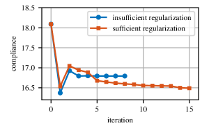
Figure 8: Convergence history of the compliance. When the regularization of $\rm J$ in line 21 of Listing 6 is insufficient, the algorithm stops after eight iterations because a triangle becomes very elongated. However, if sufficient regularization is provided, the algorithm does not experience this issue and further optimizes the design. Finally, we point out that the small value of the compliance after the first iteration is obtained by excessively violating the volume equality constraint. This is subsequently corrected by the augmented Lagrangian algorithm.

4 Shape optimization via diffeomorphisms

In this section, we describe the theory that underpins Fireshape. We begin with a brief introduction to PDE-constrained optimization to set the notation and mention the main idea behind optimization algorithms (Subsection 4.1). Then, we continue with an introduction to shape calculus (Subsection 4.2). Finally, we conclude with a discussion about the link between shape optimization and parametric finite elements (Subsection 4.3).

4.1 Optimization with PDE-constraints

The basic ingredients to formulate a PDE-constrained optimization problem are: a control variable ${\mathbf{q}}$ that lives in a control space ${\mathbf{Q}}$, a state variable ${\mathbf{u}}$ that lives in a state space ${\mathbf{U}}$ and that solves a (possibly nonlinear) state equation ${\mathbf{A}}({\mathbf{q}},{\mathbf{u}})=\mathbf{0}$, and a real function ${\rm J}:{\mathbf{Q}}\times{\mathbf{U}}\to\mathbb{R}$ to be minimized.

Example: Equation (3) is a PDE-constrained optimization problem. The control variable ${\mathbf{q}}$ corresponds to the domain $\rm\Omega$, the state variable ${\mathbf{u}}$ represents the pair velocity-pressure $({\mathbf{u}},\rm p)$, the nonlinear constraint ${\mathbf{A}}$ represents the Navier-Stokes equations (1), and $\rm J$ denotes the objective function (2). The state space ${\mathbf{U}}$ corresponds to the space of pairs $({\mathbf{a}},\rm b)$ with weakly differentiable velocities ${\mathbf{a}}$ that satisfy ${\mathbf{a}}={\mathbf{g}}$ on $\partial\rm\Omega\setminus\Gamma$ and square integrable pressures $\rm b$ (ElSiWa14, , Ch. 8.2). The control space ${\mathbf{Q}}$ is specified in Section 4.2; see Equation (7).

Most numerical methods for PDE-constrained optimization attempt to construct a sequence of controls $\{{\mathbf{q}}^{(k)}\}_{k\in\mathbb{N}}$ and corresponding states $\{{\mathbf{u}}^{(k)}\}_{k\in\mathbb{N}}$ such that

$$\lim_{k\to\infty}{\rm J}({\mathbf{q}}^{(k)},{\mathbf{u}}^{(k)})=\inf_{{\mathbf{q}},{\mathbf{u}}} \{{\rm J}({\mathbf{q}},{\mathbf{u}}):{\mathbf{A}}({\mathbf{q}},{\mathbf{u}})=\mathbf{0}\}\,.$$

Often, the sequence $\{{\mathbf{q}}^{(k)}\}_{k\in\mathbb{N}}$ is constructed using derivatives of the function ${\rm J}$ and of the constraint ${\mathbf{A}}$. Common approaches are steepest descent algorithms and Newton methods (in their quasi, Krylov, or semi-smooth versions) HiPiUlUl09 ; Ke03 . These algorithms ensure that the sequence $\{{\rm J}({\mathbf{q}}^{(k)},{\mathbf{u}}^{(k)})\}_{k\in\mathbb{N}}$ decreases. In special cases, it is even possible to show that the sequence $\{{\mathbf{q}}^{(k)}\}_{k\in\mathbb{N}}$ converges HiPiUlUl09 . Although it may be difficult to ensure these assumptions are met in industrial applications, these optimization algorithms are still powerful tools to improve state-of-the-art designs and are widely used to perform shape optimization.

4.2 Shape optimization and shape calculus

Shape optimization with PDE constraints is a particular branch of PDE-constrained optimization where the control space ${\mathbf{Q}}$ is a set of domain shapes. The space of shapes is notoriously difficult to characterize uniquely. For instance, one could describe shapes through their boundary regularity, or as level-sets, or as local epigraphs (DeZo11, , ch. 2). The choice of the shapes’ space characterization plays an important role in the concrete implementation of a shape optimization algorithm, and it can also affect formulas that result by differentiating ${\rm J}$ with respect to perturbations of the shape ${\mathbf{q}}$. To be more precise, different methods generally lead to the same first order shape derivative formula, but differ on shape derivatives of higher order (DeZo11, , ch. 9)

In this work, we model the control space ${\mathbf{Q}}$ as the images of bi-Lipschitz geometric transformations ${\mathbf{T}}$ applied to an initial set $\rm{\Omega}\subset\mathbb{R}^{d}$ (DeZo11, , ch. 3), that is,

$${\mathbf{Q}}\coloneqq\{{\mathbf{q}}={\mathbf{T}}(\rm{\Omega}):{\mathbf{T}}:\mathbb{R}^{d}\to\mathbb{R}^{d}\text{ is bi-Lipschitz}\}\,,$$ (7)

see Figure 9. We choose this model of ${\mathbf{Q}}$ because it provides an explicit description of the domain boundaries via $\partial({\mathbf{T}}(\rm{\Omega}))={\mathbf{T}}(\partial\rm{\Omega})$, and because it is compatible with higher-order finite elements PaWeFa18 , as explained in detail in the Section 4.3. Henceforth, we use the term differomorphism to indicate that a geometric transformation ${\mathbf{T}}$ is bi-Lipschitz.

Figure 9: To construct the control space ${\mathbf{Q}}$, we select an initial set $\rm{\Omega}$ and a set of diffeomorphisms $\{{\mathbf{T}}\}$ (black arrows), and collect every image ${\mathbf{T}}(\rm{\Omega})$.

In this setting, the shape derivative of ${\rm J}$ corresponds to the classical Gâteaux derivative in the Sobolev space $W^{1,\infty}(\mathbb{R}^{d},\mathbb{R}^{d})$ (HiPiUlUl09, , Def. 1.29). To see this, let us momentarily remove the PDE-constraint, and only consider a shape functional of the form $\rm{\Omega}\mapsto{\rm J}(\rm{\Omega})$. The shape derivative of ${\rm J}$ at $\rm{\Omega}$ is the linear and continuous operator $\rm{dJ}(\Omega, \cdot):W^{1,\infty}(\mathbb{R}^{d},\mathbb{R}^{d})\to\mathbb{R}$ defined by

$$\rm{dJ}(\Omega,{\mathbf{V}})\coloneqq\lim_{t\searrow 0}\frac{{\rm J}(\Omega_{t})-{\rm J}(\Omega)}{t}\,,$$ (8)

where $\rm{\Omega_{t}}$ is the set $\rm{\Omega_{t}}=\{{\mathbf{x}}+\rm{t}{\mathbf{V}}({\mathbf{x}}):{\mathbf{x}}\in\rm{\Omega}\}$ (Al07, , Def. 6.15). By replacing $\rm\Omega$ with ${\mathbf{q}}={\mathbf{I}}(\rm\Omega)$, where ${\mathbf{I}}$ denotes the identity transformation defined by ${\mathbf{I}}({\mathbf{x}})={\mathbf{x}}$ for any ${\mathbf{x}}\in\mathbb{R}^{d}$, Equation (8) can be equivalently rewritten as

$$\rm{dJ}({\mathbf{q}},{\mathbf{V}})\coloneqq\lim_{t\searrow 0}\frac{{\rm J}({\mathbf{q}}+t{\mathbf{V}})-{\rm J}({\mathbf{q}})}{t}\,.$$

We highlight that this interpretation immediately generalizes to any ${\mathbf{q}}$ in ${\mathbf{Q}}$ and can be used to define higher order shape derivatives.

The same definition (8) of shape derivative holds in the presence of PDE-constraints: the shape derivative at ${\mathbf{q}}$ of the function ${\rm J}:{\mathbf{Q}}\times{\mathbf{U}}\to\mathbb{R}$ subject to ${\mathbf{A}}({\mathbf{q}},{\mathbf{u}})=\mathbf{0}$ is the linear and continuous operator defined by

$$\rm{dJ}({\mathbf{q}},{\mathbf{u}},{\mathbf{V}})\coloneqq\lim_{t\searrow 0}\frac{{\rm J}({\mathbf{q}}+t{\mathbf{V}},{\mathbf{u}}_{t})-{\rm J}({\mathbf{q}},{\mathbf{u}})}{t}\,,$$ (9)

where ${\mathbf{u}}_{\rm t}$ is the solution to ${\mathbf{A}}({\mathbf{q}}+\rm{t}{\mathbf{V}},{\mathbf{u}}_{\rm t})=\mathbf{0}$. Computing shape derivative formulas using (9) may present the difficulty of computing the shape derivative of ${\mathbf{u}}$, which intuitively arises by the “chain rule” formula. The shape derivative of ${\mathbf{u}}$, which is sometimes called “material derivative” of ${\mathbf{u}}$, can be eliminated with the help of adjoint equations (HiPiUlUl09, , Sec. 1.6.2). This process can be automated by introducing the Lagrange functional (HiPiUlUl09, , Sec. 1.6.3)

$${\cal L}({\mathbf{q}},{\mathbf{u}},{\mathbf{p}})\coloneqq{\rm J}({\mathbf{q}},{\mathbf{u}})+\langle{\mathbf{A}}({\mathbf{q}},{\mathbf{u}}),{\mathbf{p}}\rangle\,.$$ (10)

The term $\langle{\mathbf{A}}({\mathbf{q}},{\mathbf{u}}),{\mathbf{p}}\rangle$ stems from testing the equation ${\mathbf{A}}({\mathbf{q}},{\mathbf{u}})=\mathbf{0}$ with a test function ${\mathbf{p}}$ in the same way it is usually done when writing a PDE in its weak form.

Example: If ${\mathbf{A}}$ denotes the Navier-Stokes equations (1), then $\langle{\mathbf{A}}({\mathbf{q}},{\mathbf{u}}),{\mathbf{p}}\rangle$ corresponds to the weak formulation (2.2).

The advantage of introducing the Lagrangian (10) is that, by choosing ${\mathbf{p}}$ as the solution to the adjoint equation

$$\langle\partial_{\mathbf{u}}{\mathbf{A}}({\mathbf{q}},{\mathbf{u}}),{\mathbf{p}}\rangle=-\partial_{\mathbf{u}}{\rm J}({\mathbf{q}},{\mathbf{u}})\quad\text{for all }{\mathbf{u}} \text{ in }{\mathbf{U}}\,,$$

where $\partial_{\mathbf{u}}$ denotes the partial differentiation with respect to the variable ${\mathbf{u}}$, the shape derivative of ${\rm J}$ can be computed as

$$\rm{dJ}({\mathbf{q}},{\mathbf{u}},{\mathbf{V}})=\partial_{\mathbf{q}}{\cal L}({\mathbf{q}},{\mathbf{u}},{\mathbf{p}},{\mathbf{V}})\,,$$

where $\partial_{\mathbf{q}}$ denotes partial differentiation with respect to the variable ${\mathbf{q}}$. This is advantageous because partial differentiation does not require computing the shape derivative of ${\mathbf{u}}$.

The Lagrangian approach to compute derivatives of PDE-constrained functionals is well established ItKu08 , and its steps can be replicated by symbolic computation software. Probably, the biggest success in this direction is the pyadjoint project FaHaFuRo13 ; MiFuDo19 , which derives “the adjoint and tangent-linear equations and solves them using the existing solver methods in FEniCS/Firedrake” MiFuDo19 . Thanks to the shape differentiation capabilities of UFL introduced in HaMiPaWe19 , pyadjoint is also capable of shape differentiating PDE-constrained functionals DoMiFu20 .

Remark 2

Optimization algorithms are usually based on steepest descent directions to update the control variable ${\mathbf{q}}$. A steepest descent direction is a direction ${\mathbf{V}}^{*}$ that minimizes the derivative $\rm{dJ}$. Since $\rm{dJ}$ is linear, it is necessary to introduce a norm $\|\cdot\|$ on the space of possible perturbations $\{{\mathbf{V}}\}$ (the tangent space of ${\mathbf{Q}}$ at ${\mathbf{q}}$), and to restrict the search of a steepest descent direction to directions ${\mathbf{V}}$ of length $\|{\mathbf{V}}\|=1$. A natural choice would be to select the $W^{1,\infty}$-norm, with respect to which a minimizer has been shown to exist for most functionals (PaWeFa18, , Prop. 3.1). However, in practice it is more convenient to employ a norm that is induced by an inner product, so that the steepest descent direction corresponds to the Riesz representative of $\rm{dJ}$ with respect to the inner product (HiPiUlUl09, , p. 98).

4.3 Geometric transformations, moving meshes, and parametric finite elements

To solve a PDE-constrained optimization problem iteratively, it is necessary to employ a numerical method that is capable of solving the constraint ${\mathbf{A}}({\mathbf{q}},{\mathbf{u}})=\mathbf{0}$ for any feasible control ${\mathbf{q}}$. In shape optimization, this translates into the requirement of a numerical scheme that can solve a PDE on a domain that changes at each iteration of the optimization algorithm. There are several competing approaches to construct a numerical scheme with this feature, such as the level-set method AlJoTo02 or the phase field approach BlGaFaHaSt14 , among others.

In Fireshape, we employ the approach sometimes know as “moving mesh” method PaWeFa18 ; Al07 . In its simplest version (see Figure 10), this method replaces (or approximates) the initial domain $\rm{\Omega}$ with a polygonal mesh $\rm{\Omega_{h}}$. On this mesh, the state and adjoint equations are solved with a standard finite element method, whose construction on polygonal meshes is immediate. For instance, depending on the nature of the state constraint, one may solve the state and adjoint equations using linear Lagrangian or P2-P1 Taylor-Hood finite elements (see Section 2.2). With the state and adjoint solutions at hand, one employs shape derivatives (see Remark 2 and Section 5.2) to update the coordinates of mesh nodes while retaining the mesh connectivity of $\rm\Omega_{h}$. This leads to a new mesh that represents an improved design. This update process is repeated until some prescribed convergence criteria are met.

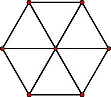
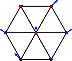
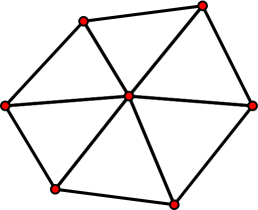
Figure 10: Simplest approach to PDE-constrained shape optimization. An initial mesh (left) is used to compute state and adjoint variables. This information, together with shape derivatives, is used to devise an update of the nodes’ coordinates (center). A new and improved initial guess is obtained by updating the nodes’ coordinates and retaining the initial mesh connectivity (right). This process is repeated until convergence.

The moving mesh method we just described is a simple and yet powerful method. However, in its current formulation, it requires polyhedral meshes, which limits the search space ${\mathbf{Q}}$ to polyhedra. In the remaining part of this section, we describe an equivalent interpretation of the moving mesh method that generalizes to curved domains. Additionally, this alternative interpretation allows approximating state and adjoint variables with arbitrarily high-order finite elements without suffering from reduction of convergence order due to poor approximation of domain boundaries (Ci02, , Ch. 4.4).

We begin by recalling the standard construction of parametric finite elements. For more details, we refer to (Ci02, , Sect. 2.3 and 4.3). To construct a parametric finite element space, one begins by partitioning the domain $\rm{\Omega}$ into simpler geometric elements $\{K_{i}\}$ (usually triangles or tetrahedra, as depicted in the first row of Figure 11). Then, one introduces a reference element $\hat{K}$ and a collection of diffeomorphisms ${\mathbf{F}}_{i}$ that map the reference element $\hat{K}$ to the various $K_{i}$s, that is, ${\mathbf{F}}_{i}(\hat{K})=K_{i}$ for every value of the index $i$ (as depicted in the second row of Figure 11). Finally, one considers a set of local reference basis functions $\{\hat{b}_{j}\}$ defined on the reference element $\hat{K}$, and defines local basis functions $\{b_{j}^{i}\}$ on each $K_{i}$ via the pullback $b_{j}^{i}({\mathbf{x}})\coloneqq\hat{b}_{j}({\mathbf{F}}_{i}^{-1}({\mathbf{x}}))$ for every ${\mathbf{x}}$ in $K_{i}$. These local basis functions are used to construct global basis functions that span the finite element space. An important property of this construction is that the diffeomorphisms ${\mathbf{F}}_{i}$ can be expressed in terms of local linear Lagrangian basis functions $\{\hat{\beta}_{m}\}$, that is, there are some coefficient vectors $\{\boldsymbol{\mu}_{m}^{i}\}$ such that

$${\mathbf{F}}_{i}({\mathbf{x}})=\sum_{m}\boldsymbol{\mu}_{m}^{i}\hat{\beta}_{m}({\mathbf{x}})\quad\text{for every} {\mathbf{x}}\text{ in }\hat{K}\,.$$ (11)

Finite elements constructed following this procedure are usually called parametric, because they rely on the parametrization $\{{\mathbf{F}}_{i}\}$. Note that the most common finite elements families, such as Lagrangian, Raviart–Thomas, or Nedelec finite elements, are indeed parametric.

Figure 11: To construct finite element basis functions, one usually begins by triangulating a domain $\rm{Omega}$ (first row) and then introducing diffeomorphisms ${\mathbf{F}}_{i}$ that map the reference element $\hat{K}$ to the various $K_{i}$ in the triangulation (second row).

Keeping this knowledge about parametric finite elements in mind, we can revisit the mesh method (see Figure 10). There, the main idea was to update only nodes’ coordinates and keep the mesh connectivity unchanged, so that constructing finite elements on the new mesh is straightforward. In PaWeFa18 , it has been shown that the new finite element space can also be obtained by modifying the parametric construction of finite elements on the original domain $\rm{\Omega}$. In the next paragraphs, we give an extended explanation (with adapted notation) of the demonstration given in PaWeFa18 .

Let ${\mathbf{T}}$ denote the transformation employed to modify the mesh $\rm\Omega_{h}$ on the left in Figure 10 into the new and perturbed mesh ${\mathbf{T}}(\rm\Omega_{h})$ on the right in Figure 10. Additionally, let $\{{\mathbf{T}}({\mathbf{K}}_{i})\}$ denote the simple geometric elements that constitute the latter. Using the parametric approach, we can construct finite elements on the new mesh by introducing a collection of diffeomorphisms $\tilde{\mathbf{F}}_{i}$ that map the reference element $\hat{K}$ to the various ${\mathbf{T}}(K_{i})$s, that is, $\tilde{\mathbf{F}}_{i}(\hat{K})={\mathbf{T}}(K_{i})$ for every value of the index $i$; see Figure 12.

Figure 12: The standard construction of finite elements on the perturbed mesh $\{{\mathbf{T}}(K_{i})\}$ employs diffeomorphisms $\tilde{\mathbf{F}}_{i}$ that map the reference element $\hat{K}$ to the various perturbed elements ${\mathbf{T}}(K_{i})$.

The behavior of the transformation ${\mathbf{T}}$ in Figure 10 is prescribed only the mesh nodes. Since its behavior on the interior of the mesh triangles can be chosen arbitrarily, we can decide that ${\mathbf{T}}$ is piecewise affine on each triangle. This convenient choice implies that ${\mathbf{T}}$ can be written as a linear combination of piecewise affine Lagrangian finite elements defined on the first mesh, that is, ${\mathbf{T}}({\mathbf{x}})=\sum_{\ell}\boldsymbol{\nu}_{\ell}B_{\ell}({\mathbf{x}})$ for every ${\mathbf{x}}$ in $\rm{\Omega}$, where $\{\boldsymbol{\nu}_{\ell}\}$ are some coefficient vectors and $\{B_{\ell}\}$ are global basis functions of the space of piecewise affine Lagrangian finite elements defined on the partition $\{K_{i}\}$. Since Lagrangian finite elements are constructed via pullbacks to the reference element, for every element $K_{i}$ there are coefficient vectors $\{\boldsymbol{\nu}_{m}^{i}\}$ so that the restriction ${\mathbf{T}}|_{K_{i}}$ of ${\mathbf{T}}$ on $K_{i}$ can be rewritten as

$${\mathbf{T}}|_{K_{i}}({\mathbf{x}})=\sum_{\ell}\boldsymbol{\nu}_{\ell}B_{\ell}|_{K_{i}}({\mathbf{x}})=\sum_{m}\tilde{\boldsymbol{\nu}}_{m}^{i}\hat{\beta}_{m}({\mathbf{F}}_{i}^{-1}({\mathbf{x}}))\,.$$

Therefore, the composition ${\mathbf{T}}|_{K_{i}}\circ{\mathbf{F}}_{i}$ is of the form

$${\mathbf{T}}|_{K_{i}}\circ{\mathbf{F}}_{i}({\mathbf{x}})=\sum_{m}\tilde{\boldsymbol{\nu}}_{m}^{i}\hat{\beta}_{m}({\mathbf{x}})\quad\text{for every }{\mathbf{x}}\in\hat{K}\,,$$ (12)

that is, of the same form of Equation (11). This implies that, to construct finite elements on the perturbed geometry ${\mathbf{T}}(\rm{\Omega}_{h})$, we only need to replace the original coefficients $\{\boldsymbol{\mu}_{m}^{i}\}$ in Equation (11) with the new coefficients $\{\tilde{\boldsymbol{\nu}}_{m}^{i}\}$ from Equation (12).

This alternative and equivalent viewpoint on the moving mesh method generalizes naturally to higher-order finite element approximations of control and state (and adjoint) variables. Indeed, one of the key steps to ensure that higher-order finite elements achieve higher-order convergence on curved domains is to employ sufficiently accurate polynomial interpolation of domain boundaries (Ci02, , Ch. 4.4). This boundary interpolation can be encoded in the diffeomorphisms $\{{\mathbf{F}}_{i}\}$ by using higher-order Lagrangian local basis functions. Therefore, simply employing higher-order Lagrangian finite element transformations ${\mathbf{T}}$ leads to a natural extension of moving mesh method to higher-order finite elements.

This alternative and equivalent viewpoint generalizes further to allow the use of any arbitrary discretization of the transformation ${\mathbf{T}}$ (for instance, using B-splines Ho03 , harmonic polynomials, or radial basis functions We05 ). The only requirement to be fulfilled to ensure the desired order of convergence $p$ is that the maps ${\mathbf{T}}\circ{\mathbf{F}}_{i}:{\mathbf{x}}\mapsto{\mathbf{T}}({\mathbf{F}}_{i}({\mathbf{x}}))$ satisfy the asymptotic algebraic estimates

$$\|{\mathbf{D}}^{\alpha}({\mathbf{T}}\circ{\mathbf{F}}_{i})\|={\cal O}(h^{\alpha})\quad\text{for }0\leq\alpha\leq p\,,$$

where ${\mathbf{D}}^{\alpha}({\mathbf{T}}\circ{\mathbf{F}}_{i})$ denotes the $\alpha^{\rm{th}}$ derivative of ${\mathbf{T}}\circ{\mathbf{F}}_{i}$. Using a different discretization of the transformation ${\mathbf{T}}$ can give several advantages, like increasing the smoothness ${\mathbf{T}}$ (because finite elements are generally only Lipschitz continuous) or varying how shape updates are computed during the optimization process EiSt18 .

Remark 3

An issue that can arise with the moving mesh method is that it can lead to poor quality (or even tangled) meshes. In terms of geometric transformations, a mesh with poor quality corresponds to a transformation ${\mathbf{T}}$ for which the value $\max_{\alpha}\|{\mathbf{D}}^{\alpha}{\mathbf{T}}\|$ is large (and a tangled mesh to a transformation ${\mathbf{T}}$ that is not a diffeomorphism). To a certain extent, it is possible to enforce moderate derivatives by employing suitable metrics to extract descent directions from shape derivatives (for instance, by using linear elasticity based inner products with a Cauchy-Riemann augmentation IgStWe18 ) and/or by adding penalty terms to the functional ${\rm J}$. For example, in Sections 2.4 and 3.4 we add a penalization term based on the spectral norm $\|{\mathbf{D}}({\mathbf{T}}-{\mathbf{I}})\|_{2}$ of the Jacobian matrix ${\mathbf{D}}({\mathbf{T}}-{\mathbf{I}})$. We point out that if $\rm\Omega$ is $\zeta$-quasiconvex and $\|{\mathbf{D}}({\mathbf{T}}-{\mathbf{I}})\|_{2}<\zeta$, then ${\mathbf{T}}:{\rm\Omega}\to\mathbb{R}^{d}$ is bi-Lipschitz, and thus injective.

5 Anatomy of Fireshape

In this section, we give more details about Fireshape’s implementation and features. Fireshape is organized in a few core Python classes (and associated subclasses) that implement the control space ${\mathbf{Q}}$, the metric to be employed by the optimization algorithm, and the (possibly PDE-constrained) objective function $\rm{J}$. The following subsections describe these classes.

5.1 The class ControlSpace

Fireshape models the control space ${\mathbf{Q}}$ of admissible domains using geometric transformations ${\mathbf{T}}$ as in Equation (7) (see also Figure 9). From a theoretical perspective, the transformations ${\mathbf{T}}$ can be discretized in numerous different ways as long as certain minimal regularity requirements are met. In Fireshape, the class ControlSpace allows the following options: (i) Lagrangian finite elements defined on the same mesh employed to solve the state equation, (ii) Lagrangian finite elements defined on a mesh coarser than the mesh employed to solve the state equation, and (iii) tensorized B-splines defined on a separate Cartesian grid (not to be confused with a spline or Bézier parametrization of the domain boundary, see Figure 13). In this case, the user must specify the boundary and the refinement level of the Cartesian grid (bbox and level), as well as the order of the underlying univariate B-splines. The user can also set the regulariy of B-splines on the boundary of the Cartesian grid (voundary_regularities), or restrict pertubations to specific directions (fixed_dims).

Figure 13: Fireshape allows discretizing transformations ${\mathbf{T}}$ using tensorized B-splines. On the left, we display a Cartesian grid that that covers the computational domain $\rm{\Omega}$. On the right, we display a quadratic tensorized B-spline.

If discretization (i) can be considered to be the default option, discretization (ii) allows introducing a regularization by discretizing the geometry more coarsely (so-called “regularization by discretization”), whereas B-splines allow constructing transformation with higher regularity (Lagrangian finite elements are only Lipschitz continuous, whereas B-splines can be continuously differentiable and more).

The class ControlSpace can be easily extended to include additional discretization options, such as radial basis functions and harmonic polynomials.

Remark 4

The current implementation of the control space ${\mathbf{Q}}$ includes geometric transformations that can leave the value of a shape function unchanged. For instance, if ${\rm J}(\rm{\Omega})=\int_{\rm{\Omega}}\,\mathrm{d}{\boldsymbol{x}}$, then any diffeomorphism ${\mathbf{T}}$ of the form ${\mathbf{T}}={\mathbf{I}}+{\mathbf{V}}$ with ${\mathbf{V}}\neq\mathbf{0}$ in $\rm{\Omega}$ and ${\mathbf{V}}=\mathbf{0}$ on $\rm{\partial\Omega}$ satisfy ${\mathbf{T}}(\rm{\Omega})=\rm{\Omega}$, and thus ${\rm J}({\mathbf{T}}(\rm{\Omega}))={\rm J}(\rm{\Omega})$.

The presence of a shape function kernel in the control space ${\mathbf{Q}}$ does not represent a problem for steepest descent and quasi Newton optimization algorithms. However, this kernel leads to singular Hessians, and Newton’s method cannot be applied in a straightforward fashion. The development of control space descriptions that exclude shape function kernels and allow direct applications of shape Newton methods in the framework of finite element simulations is a highly active research field sturm2016convergence ; paganini2019weakly ; EtHeLoWa20 . We predict these new control spaces will be included in Fireshape as soon as their description has been established.

5.2 The class InnerProduct

To formulate a continuous optimization algorithm, we need to specify how to compute lengths of vectors (and, possibly, how to compute the angle between two vectors). The class InnerProduct addresses this requirement and allows selecting an inner product $(\cdot,\cdot)_{\cal H}$ to endow the control space ${\mathbf{Q}}$ with.

The choice of the inner product affects how steepest-descent directions are computed. Indeed, a steepest-descent direction is a direction ${\mathbf{V}}$ of length $\|{\mathbf{V}}\|_{\cal H}=1$ such that $\rm{dJ}({\mathbf{q}},{\mathbf{V}})$ is minimal. Let $\alpha\coloneqq\|\rm{dJ}({\mathbf{q}},\cdot)\|_{*}$ denote the length of the operator $\rm{dJ}({\mathbf{q}},\cdot)$ measured with respect to the dual norm. Then (HiPiUlUl09, , p. 103), the steepest descent direction ${\mathbf{V}}$ satisfies the equation

$$\alpha({\mathbf{V}},{\mathbf{W}})_{\cal H}=-\rm{dJ}({\mathbf{q}},{\mathbf{W}})\quad\text{for all }{\mathbf{W}}\text{ in }{\cal H}\,,$$

which clearly depends on the inner product $(\cdot,\cdot)_{\cal H}$.

The control space ${\mathbf{Q}}$ can be endowed with different inner products. In Fireshape, the class InnerProduct allows the following options: (i) an $H^{1}(\rm{\Omega})$ inner product based on standard Galerkin stiffness and mass matrices, (ii) a Laplace inner product based on the Galerkin stiffness matrix, and (iii) an elasticity inner product based on the linear elasticity mechanical model. These options can be complemented with additional homogeneous Dirichlet boundary conditions to specify parts of the boundary $\partial\rm{\Omega}$ that are not to be modified during the shape optimization procedure.

Although all three options are equivalent from a theoretical perspective, in practice it has been observed that option (iii) generally leads to geometry updates that result in meshes of higher equality compared to options (i) and (ii). A thorough comparison is available in IgStWe18 , where the authors also suggest to consider complementing these inner products with terms stemming from Cauchy-Riemann equations to further increase mesh quality. This additional option is readily available in Fireshape.

5.3 The classes Objective and PdeConstraint

In the vast majority of cases, users who aim to solve a PDE-constrained shape optimization problem are only required to instantiate the two classes Objective and PdeConstraint, where they can specify the formula of the function $\rm{J}$ to be minimized and the weak formulation of its PDE-constraint ${\mathbf{A}}(\rm{\Omega},{\mathbf{u}})=\mathbb{0}$ (see Sections 2.2 and 2.3, for instance). Since Fireshape is built on top of the finite element library Firedrake, these formulas must be written using the Unified Form Language (UFL). We refer to the tutorials on the website Firedrakewebsite for more details about Firedrake and UFL.

5.4 Supplementary classes

Fireshape also includes a few extra classes to specify additional constraints, such as volume or perimeter constraints on the domain $\rm{\Omega}$, or spectral constraints to control the singular values of the transformation ${\mathbf{T}}$. For more details about these extra options, we refer to Fireshape’s documentation and tutorials Fireshapedocu .

6 Conclusions

We have introduced Fireshape: an open-source and automated shape optimization toolbox for the finite element software Firedrake. Fireshape is based on the moving mesh method and allows users with minimal shape optimization knowledge to tackle challenging shape optimization problems constrained to PDEs. In particular, Fireshape computes adjoint equations and shape derivatives in an automated fashion, allows decoupled discretizations of control and state variables, and gives full access to Firedrake’s and PETSc’s discretization and solver capabilities as well as to the extensive optimization library ROL.

References

- (1) Abramowski, T., Sugalski, K.: Energy saving procedures for fishing vessels by means of numerical optimization of hull resistance. Zeszyty Naukowe Akademii Morskiej w Szczecinie (2017)
- (2) Ahrens, J., Geveci, B., Law, C.: Paraview: An end-user tool for large data visualization. The visualization handbook 717 (2005)
- (3) Allaire, G.: Conception optimale de structures, Mathematics & Applications, vol. 58. Springer-Verlag, Berlin (2007)
- (4) Allaire, G., Jouve, F., Toader, A.M.: A level-set method for shape optimization. C. R. Math. Acad. Sci. Paris 334(12), 1125–1130 (2002)
- (5) Allaire, G., Pantz, O.: Structural optimization with FreeFem++. Struct. Multidiscip. Optim. 32(3), 173–181 (2006)
- (6) Alnæs, M.S., Logg, A., Ølgaard, K.B., Rognes, M.E., Wells, G.N.: Unified Form Language: A Domain-specific Language for Weak Formulations of Partial Differential Equations. ACM Transactions on Mathematical Software 40(2), 9:1–9:37 (2014). DOI 10.1145/2566630
- (7) Amestoy, P.R., Duff, I.S., L’Excellent, J.Y., Koster, J.: MUMPS: a general purpose distributed memory sparse solver. In: International Workshop on Applied Parallel Computing, pp. 121–130. Springer (2000). DOI 10.1007/3-540-70734-4˙16
- (8) Balay, S., Abhyankar, S., Adams, M.F., Brown, J., Brune, P., Buschelman, K., Dalcin, L., Eijkhout, V., Gropp, W.D., Karpeyev, D., Kaushik, D., Knepley, M.G., May, D.A., McInnes, L.C., Mills, R.T., Munson, T., Rupp, K., Sanan, P., Smith, B.F., Zampini, S., Zhang, H., Zhang, H.: PETSc users manual. Tech. Rep. ANL-95/11 - Revision 3.11, Argonne National Laboratory (2019)
- (9) Balay, S., Gropp, W.D., McInnes, L.C., Smith, B.F.: Efficient management of parallelism in object oriented numerical software libraries. In: E. Arge, A.M. Bruaset, H.P. Langtangen (eds.) Modern Software Tools in Scientific Computing, pp. 163–202. Birkhäuser Press (1997)
- (10) Bendsøe, M.P.: Optimal shape design as a material distribution problem. Structural optimization 1(4), 193–202 (1989)
- (11) Bendsoe, M.P., Sigmund, O.: Topology Optimization: Theory, Methods and Applications. Springer (2004)
- (12) Bernland, A., Wadbro, E., Berggren, M.: Shape optimization of a compression driver phase plug. SIAM J. Sci. Comput. 41(1), B181–B204 (2019). DOI 10.1137/18M1175768. URL https://doi.org/10.1137/18M1175768
- (13) Blank, L., Garcke, H., Farshbaf-Shaker, M.H., Styles, V.: Relating phase field and sharp interface approaches to structural topology optimization. ESAIM Control Optim. Calc. Var. 20(4), 1025–1058 (2014)
- (14) Braess, D.: Finite elements, third edn. Cambridge University Press, Cambridge (2007)
- (15) Chevalier, C., Pellegrini, F.: PT-SCOTCH: a tool for efficient parallel graph ordering. Parallel Computing 34(6), 318–331 (2008)
- (16) Ciarlet, P.G.: The finite element method for elliptic problems. Society for Industrial and Applied Mathematics (SIAM), Philadelphia, PA (2002)
- (17) Courtais, A., Lesage, F., Privat, Y., Frey, P., razak Latifi, A.: Adjoint system method in shape optimization of some typical fluid flow patterns. In: A.A. Kiss, E. Zondervan, R. Lakerveld, L. Özkan (eds.) 29th European Symposium on Computer Aided Process Engineering, Computer Aided Chemical Engineering, vol. 46, pp. 871 – 876. Elsevier (2019)
- (18) Dalcin, L.D., Paz, R.R., Kler, P.A., Cosimo, A.: Parallel distributed computing using Python. Advances in Water Resources 34(9), 1124–1139 (2011). New Computational Methods and Software Tools
- (19) Dapogny, C., Faure, A., Michailidis, G., Allaire, G., Couvelas, A., Estevez, R.: Geometric constraints for shape and topology optimization in architectural design. Comput. Mech. 59(6), 933–965 (2017)
- (20) Dapogny, C., Frey, P., Omnès, F., Privat, Y.: Geometrical shape optimization in fluid mechanics using FreeFem++. Struct. Multidiscip. Optim. 58(6), 2761–2788 (2018)
- (21) Delfour, M.C., Zolésio, J.P.: Shapes and geometries. Metrics, analysis, differential calculus, and optimization, Advances in Design and Control, vol. 22, second edn. Society for Industrial and Applied Mathematics (SIAM), Philadelphia, PA (2011)
- (22) Denis Rldzal, D.K.: Rapid optimization library, version 00 (2014). URL https://www.osti.gov//servlets/purl/1232084
- (23) Dilgen, C.B., Dilgen, S.B., Fuhrman, D.R., Sigmund, O., Lazarov, B.S.: Topology optimization of turbulent flows. Comput. Methods Appl. Mech. Engrg. 331, 363–393 (2018)
- (24) Dokken, J.S., Funke, S.W., Johansson, A., Schmidt, S.: Shape optimization using the finite element method on multiple meshes with nitsche coupling. SIAM Journal on Scientific Computing 41(3), A1923–A1948 (2019)
- (25) Dokken, J.S., Mitusch, S.K., Funke, S.W.: Automatic shape derivatives for transient PDEs in FEniCS and Firedrake (2020)
- (26) Dondl, P., Poh, P.S.P., Rumpf, M., Simon, S.: Simultaneous elastic shape optimization for a domain splitting in bone tissue engineering. Proc. A. 475(2227), 20180718, 17 (2019). DOI 10.1098/rspa.2018.0718. URL https://doi.org/10.1098/rspa.2018.0718
- (27) Eigel, M., Sturm, K.: Reproducing kernel hilbert spaces and variable metric algorithms in pde-constrained shape optimization. Optimization Methods and Software 33(2), 268–296 (2018)
- (28) Elman, H.C., Silvester, D.J., Wathen, A.J.: Finite elements and fast iterative solvers: with applications in incompressible fluid dynamics, second edn. Oxford University Press, Oxford (2014)
- (29) Etling, T., Herzog, R., Loayza, E., Wachsmuth, G.: First and second order shape optimization based on restricted mesh deformations. SIAM Journal on Scientific Computing 42(2), A1200–A1225 (2020)
- (30) Farrell, P.E., Ham, D.A., Funke, S.W., Rognes, M.E.: Automated derivation of the adjoint of high-level transient finite element programs. SIAM J. Sci. Comput. 35(4), C369–C393 (2013)
- (31) Farrell, P.E., Mitchell, L., Wechsung, F.: An augmented lagrangian preconditioner for the 3d stationary incompressible navier–stokes equations at high reynolds number. SIAM Journal on Scientific Computing 41(5), A3073–A3096 (2019)
- (32) Feppon, F., Allaire, G., Dapogny, C., Jolivet, P.: Topology optimization of thermal fluid-structure systems using body-fitted meshes and parallel computing. J. Comput. Phys. 417, 109574, 30 (2020)
- (33) Firedrake, project website. https://www.firedrakeproject.org/
- (34) Fireshape, documentation. https://fireshape.readthedocs.io/en/latest/index.html
- (35) Garcke, H., Hecht, C., Hinze, M., Kahle, C.: Numerical approximation of phase field based shape and topology optimization for fluids. SIAM Journal on Scientific Computing 37(4), A1846–A1871 (2015)
- (36) Geuzaine, C., Remacle, J.F.: Gmsh: A 3-d finite element mesh generator with built-in pre-and post-processing facilities. International journal for numerical methods in engineering 79(11), 1309–1331 (2009)
- (37) Gibson, T.H., Mitchell, L., Ham, D.A., Cotter, C.J.: A domain-specific language for the hybridization and static condensation of finite element methods (2018). URL https://arxiv.org/abs/1802.00303
- (38) Ham, D.A., Mitchell, L., Paganini, A., Wechsung, F.: Automated shape differentiation in the Unified Form Language. Struct. Multidiscip. Optim. 60(5), 1813–1820 (2019)
- (39) He, X., Li, J., Mader, C.A., Yildirim, A., Martins, J.R.: Robust aerodynamic shape optimization—from a circle to an airfoil. Aerospace Science and Technology 87, 48–61 (2019)
- (40) Hinze, M., Pinnau, R., Ulbrich, M., Ulbrich, S.: Optimization with PDE constraints, Mathematical Modelling: Theory and Applications, vol. 23. Springer, New York (2009)
- (41) Höllig, K.: Finite element methods with B-splines. Society for Industrial and Applied Mathematics (SIAM), Philadelphia, PA (2003)
- (42) Homolya, M., Kirby, R.C., Ham, D.A.: Exposing and exploiting structure: optimal code generation for high-order finite element methods (2017). URL http://arxiv.org/abs/1711.02473
- (43) Homolya, M., Mitchell, L., Luporini, F., Ham, D.A.: TSFC: a structure-preserving form compiler (2017). URL http://arxiv.org/abs/1705.003667
- (44) Iglesias, J.A., Sturm, K., Wechsung, F.: Two-dimensional shape optimization with nearly conformal transformations. SIAM Journal on Scientific Computing 40(6), A3807–A3830 (2018)
- (45) Ito, K., Kunisch, K.: Lagrange multiplier approach to variational problems and applications, Advances in Design and Control, vol. 15. Society for Industrial and Applied Mathematics (SIAM), Philadelphia, PA (2008)
- (46) Kelley, C.T.: Solving nonlinear equations with Newton’s method, Fundamentals of Algorithms, vol. 1. Society for Industrial and Applied Mathematics (SIAM), Philadelphia, PA (2003)
- (47) Laurain, A.: A level set-based structural optimization code using FEniCS. Struct. Multidiscip. Optim. 58(3), 1311–1334 (2018)
- (48) Lawrence Livermore National Laboratory: hypre: High Performance Preconditioners. https://computation.llnl.gov/projects/hypre-scalable-linear-solvers-multigrid-methods
- (49) Liu, Z., Korvink, J., Huang, R.: Structure topology optimization: fully coupled level set method via femlab. Structural and Multidisciplinary Optimization 29(6), 407–417 (2005)
- (50) Lombardi, M., Parolini, N., Quarteroni, A., Rozza, G.: Numerical simulation of sailing boats: dynamics, fsi, and shape optimization. In: Variational Analysis and Aerospace Engineering: Mathematical Challenges for Aerospace Design, pp. 339–377. Springer (2012)
- (51) Luporini, F., Ham, D.A., Kelly, P.H.J.: An algorithm for the optimization of finite element integration loops. ACM Transactions on Mathematical Software 44, 3:1–3:26 (2017)
- (52) Marinić-Kragić, I., Vučina, D., Ćurković, M.: Efficient shape parameterization method for multidisciplinary global optimization and application to integrated ship hull shape optimization workflow. Computer-Aided Design 80, 61–75 (2016)
- (53) Mitchell, L., Müller, E.H.: High level implementation of geometric multigrid solvers for finite element problems: Applications in atmospheric modelling. Journal of Computational Physics 327, 1–18 (2016). DOI 10.1016/j.jcp.2016.09.037
- (54) Mitusch, S.K., Funke, S.W., Dokken, J.S.: dolfin-adjoint 2018.1: automated adjoints for FEniCS and Firedrake. The Journal of Open Source Software 4 (2019)
- (55) Nocedal, J., Wright, S.J.: Numerical optimization, second edn. Springer, New York (2006)
- (56) Paganini, A., Sturm, K.: Weakly normal basis vector fields in rkhs with an application to shape newton methods. SIAM Journal on Numerical Analysis 57(1), 1–26 (2019)
- (57) Paganini, A., Wechsung, F., Farrell, P.E.: Higher-order moving mesh methods for PDE-constrained shape optimization. SIAM J. Sci. Comput. 40(4), A2356–A2382 (2018)
- (58) Rathgeber, F., Ham, D.A., Mitchell, L., Lange, M., Luporini, F., McRae, A.T.T., Bercea, G.T., Markall, G.R., Kelly, P.H.J.: Firedrake: automating the finite element method by composing abstractions. ACM Trans. Math. Softw. 43(3), 24:1–24:27 (2016)
- (59) Schmidt, S., Ilic, C., Schulz, V., Gauger, N.R.: Three-dimensional large-scale aerodynamic shape optimization based on shape calculus. AIAA journal 51(11), 2615–2627 (2013)
- (60) Schulz, V., Gherman, I.: One-shot methods for aerodynamic shape optimization. In: MEGADESIGN and MegaOpt-German Initiatives for Aerodynamic Simulation and Optimization in Aircraft Design, pp. 207–220. Springer (2009)
- (61) Sigmund, O.: A 99 line topology optimization code written in matlab. Struct. Multidiscip. Optim. 21(2), 120–127 (2001)
- (62) Sturm, K.: Convergence of newton’s method in shape optimisation via approximate normal functions. arXiv preprint arXiv:1608.02699 (2016)
- (63) Talischi, C., Paulino, G.H., Pereira, A., Menezes, I.F.: Polytop: a matlab implementation of a general topology optimization framework using unstructured polygonal finite element meshes. Structural and Multidisciplinary Optimization 45(3), 329–357 (2012)
- (64) Villanueva, C.H., Maute, K.: CutFEM topology optimization of 3D laminar incompressible flow problems. Comput. Methods Appl. Mech. Engrg. 320, 444–473 (2017)
- (65) Wang, H., Doherty, J., Jin, Y.: Hierarchical surrogate-assisted evolutionary multi-scenario airfoil shape optimization. In: 2018 IEEE Congress on Evolutionary Computation (CEC), pp. 1–8. IEEE (2018)
- (66) Wechsung, F.: Shape optimisation and robust solvers for incompressible flow. Ph.D. thesis, University of Oxford (2019)
- (67) Wendland, H.: Scattered data approximation. Cambridge University Press, Cambridge (2005)
- (68) Software used in ’Fireshape: a shape optimization toolbox for Firedrake’ (2020). DOI 10.5281/zenodo.4036176. URL https://doi.org/10.5281/zenodo.4036176
- (69) Fireshape: a shape optimization toolbox for Firedrake (2020). DOI 10.5281/zenodo.4036213. URL https://doi.org/10.5281/zenodo.4036213
- (70) Zhou, S., Li, Q.: A variational level set method for the topology optimization of steady-state Navier-Stokes flow. J. Comput. Phys. 227(24), 10178–10195 (2008). DOI 10.1016/j.jcp.2008.08.022. URL https://doi.org/10.1016/j.jcp.2008.08.022