Optimal Cybersecurity Investments in Large Networks Using SIS Model: Algorithm Design

Abstract

We study the problem of minimizing the (time) average security costs in large networks/systems comprising many interdependent subsystems, where the state evolution is captured by a susceptible-infected-susceptible (SIS) model. The security costs reflect security investments, economic losses and recovery costs from infections and failures following successful attacks. We show that the resulting optimization problem is nonconvex and propose a suite of algorithms – two based on a convex relaxation, and the other two for finding a local minimizer, based on a reduced gradient method and sequential convex programming. Also, we provide a sufficient condition under which the convex relaxations are exact and, hence, their solution coincides with that of the original problem. Numerical results are provided to validate our analytical results and to demonstrate the effectiveness of the proposed algorithms.

1 Introduction

Today, many modern engineered systems, including information and communication networks and power systems, comprise many interdependent systems. For uninterrupted delivery of their services, the comprising systems must work together and oftentimes support each other. Unfortunately, this interdependence among comprising systems also introduces a source of vulnerability in that it is possible for a local failure or infection of a system by malware to spread to other systems, potentially compromising the integrity of the overall system. Analogously, in social networks, contagious diseases often spread from infected individuals to other vulnerable individuals through contacts or physical proximity.

From this viewpoint, it is clear that the underlying networks that govern the interdependence among systems have a large impact on dynamics of the spread of failures or malware infections. Similarly, the topology and contact frequencies among individuals in social networks significantly influence the manner in which diseases spread in societies. Thus, any sound investments in security of complex systems or the control of epidemics should take into account the interdependence in the systems and social contacts in order to maximize potential benefits from the investments.

In our model, attacks targeting the systems arrive according to some (stochastic) process. Successful attacks on the systems can also spread from infected systems to other systems via aforementioned dependence among the systems. The system operator decides appropriate security investments to fend off the attacks, which in turn determine their breach probability, i.e., the probability that they fall victim to attacks and become infected.

Our goal is to minimize the (time) average costs of a system operator managing a large system comprising many systems, such as large enterprise intranets. The overall costs in our model account for both security investments and recovery/repair costs ensuing infections or failures, which we call infection costs in the paper. To this end, we first consider a scenario where malicious actors launch external or primary attacks. When a primary attack on a system is successful, the infected system can spread it to other systems, which we call secondary attacks by the infected systems, to distinguish them from primary attacks. When primary attacks do not stop, it is in general not possible to achieve an infection-free state at steady state.

In the second case, we assume that there are no primary attacks and examine the steady state, starting with an initial state where some systems are infected. The goal of studying this scenario is to get additional insights into scenarios where the primary attacks occur infrequently. It turns out that, even in the absence of primary attacks, infections may persist due to secondary attacks and the system may not be able to attain the infection-free steady state, and we can compute an upper bound on the optimal value, which is also tight under some condition, more easily.

We formulate the problem of determining the optimal security investments that minimize the average costs as an optimization problem. Unfortunately, this optimization problem is nonconvex and cannot be solved easily. In order to gauge the quality of a feasible solution, we obtain both a lower bound and an upper bound on the optimal value of our problem. A lower bound can be acquired using one of two different convex relaxations of the original problem we propose. For the convex relaxations, we also derive a sufficient condition under which the solution of the convex relaxation solves the original nonconvex optimization problem (Lemma 3). An upper bound on the optimal value can be obtained using an algorithm that finds a local minimizer. Here, we propose two methods – a reduced gradient method (RGM) and sequential convex programming (SCP), both of which produce a local minimizer. Together, our approach offers a bound on the optimality gap.

Numerical studies show that the computational requirements for the proposed methods are light to modest even for large systems, except for one method, which requires the calculation of an inverse matrix. They suggest that, in almost all cases that we considered, the gap between the lower bound on the optimal value and the cost achieved by our solutions is small; in fact, in most cases, the gap is less than 2-3 percent with the gap being less than 0.3 percent in many cases. In addition, when the infection costs are large, which are likely true in many practical scenarios, the sufficient condition for the convex relaxations to be exact holds, and we obtain optimal points by solving the convex relaxations. Finally, the RGM is computationally most efficient (with the computational time being less than two seconds in all considered cases and less than 0.1 seconds in most cases) and the quality of solutions is on par with that of other methods. This suggests that the RGM may offer a good practical solution for our problem.

1.1 Related Literature

Given the importance of cybersecurity, robustness of complex systems, and control of epidemics, there is already a large body of literature that examines how to optimize the (security) investments in complex systems [15, 22], the mitigation of disease or infection spread [7, 11, 30], feasibility and case studies of cyber insurance using pre-screening or differentiated pricing based on the security investments of the insured [33, 16], and designing good attack models and effective mitigating defense against attacks [29, 27, 40]. In view of the volume of existing literature, here we summarize only a small set of studies most closely related to our study.

In [17, 20, 22, 14], the authors adopted a game theoretic formulation to study the problem of security investments with distributed agents or autonomous systems that do not coordinate their efforts. The problem we study in this paper is complementary, but is very different from those studied in the aforementioned studies: in our setting, we assume that the system is managed by a single operator and is interested in minimizing the average (security) costs over time by determining (nearly) optimal security investments. Our study is applicable to, for example, the problem of finding suitable security investments in large enterprise intranets supporting common business processes or supervisory control and data acquisition systems comprising many subsystems.

In another line of research, which is most closely related to our study, researchers investigated optimal strategies using vaccines/immunization (prevention) [7, 36], antidotes or curing rates (recovery) [4, 25, 32] or a combination of both preventive and recovery measures [30, 37]. For example, [36] studies the problem of partial vaccination via investments at each individual to reduce the infection rates, with the aim of maximizing the exponential decay rate to control the spread of an epidemic. Similarly, [25] examines the problem of determining the optimal curing rates for distributed agents under different formulations. In particular, the last formulation of the problem [25], for which only partial result is obtained, is closely related to a special case of our formulation studied in Section 6.

Key differences between existing studies, including those listed above, and ours can be summarized as follows: first, unlike previous studies that focus on either the expected costs from single or cascading failures/infections [22, 19, 20] or the exponential decay rate to the disease-free state as a key performance metric, we aim to minimize the (time) average costs of a system operator, while accounting for both security investments and infection costs, with both primary and secondary attacks, by modeling time-varying states of systems due to the transmissions of failures/infections. In the presence of primary attacks, it is in general not possible to achieve the infection-free steady state and, thus, the exponential decay rate is no longer a suitable performance metric for our study. Second, unlike some studies that assume that the expected costs/risks seen by systems are convex functions of security investments (e.g., [15]), the expected risks are derived from the steady state equilibrium of a differential system that describes system states and depends on security investments. As it will be clear, the lack of a closed-form expression for the steady state equilibrium complicates considerably the analysis and algorithm design.

Preliminary results of this paper were reported in [26]. In this paper, we extend the findings of [26] in several significant directions. First, we offer an alternative convex relaxation of the original problem. As we demonstrate, this new relaxation technique based on exponential cones, is more efficient and avoids the key issues of the approach based on M-matrix theory presented in [26]. Second, we present another computationally efficient approach to finding a suboptimal solution using SCP together with our M-matrix theory-based approach, which provides an upper bound on the optimal value of the original nonconvex optimization problem. We compare this approach to one based on the RGM and show that the quality of solutions from these two methods is comparable, but the RGM holds a slight computational edge. Finally, we study a special case with no primary attacks, which is related to the epidemic control problem studied in [28, 25, 32]. Although this can be viewed as a limit case of our problem formulation as the rates of primary attacks go to zero, our approaches to obtaining upper and lower bounds of the optimal value require significant modifications for the reason explained in Section 6. Moreover, we derive sufficient conditions for optimality, which can be verified relatively easily.

The rest of the paper is organized as follows: Section 2 explains the notation and terminology we adopt. Section 3 describes the setup and the problem formulation, including the optimization problem. Section 4 discusses two different convex relaxations of the original problem, followed by two methods for finding local minimizers in Section 5. We discuss a special case with no primary attacks in Section 6. Numerical results are provided in Section 7, followed by a discussion on how our formulation and results can be extended in Section 8. We conclude in Section 9.

2 Preliminaries

2.1 Notation and Terminology

Let $\mathbb{R}$ and $\mathbb{R}_{+}$ denote the set of real numbers and nonnegative real numbers, respectively. Given a set $\mathbb{A}$, we denote the closure, interior, and boundary of $\mathbb{A}$ by cl$(\mathbb{A})$, int$(\mathbb{A})$, and $\partial\mathbb{A}$, respectively.

For a matrix $A=[a_{i,j}]$, let $a_{i,j}$ denote its $(i,j)$ element, $A^{\mathsf{T}}$ its transpose, $\rho(A)$ its spectral radius, and $\underline{\sigma}(A)$ and $\bar{\sigma}(A)$ the smallest and largest real parts of its eigenvalues. For two matrices $A$ and $B$, we write $A\!\geq\!B$ if $A\!-\!B$ is a nonnegative matrix. We use boldface letters to denote vectors, e.g., ${\mathbf{x}}\!=\![x_{1},...,x_{n}]^{\mathsf{T}}$ and $\mathbf{1}\!=\![1,...,1]^{\mathsf{T}}$. For any two vectors ${\mathbf{x}}$ and $\mathbf{y}$ of the same dimension, ${\mathbf{x}}\circ\mathbf{y}$ and $\frac{{\mathbf{x}}}{\mathbf{y}}$ are their element-wise product and division, respectively. For ${\mathbf{x}}\in\mathbb{R}^{n}$, $\mathtt{diag}({\mathbf{x}})\in\mathbb{R}^{n\times n}$ denotes the diagonal matrix with diagonal elements $x_{1},\ldots,x_{n}$.

A directed graph $\mathcal{G}\!=\!(\mathcal{V},\mathcal{E})$ consists of a set of nodes $\mathcal{V}$, and a set of directed edges $\mathcal{E}\subseteq\mathcal{V}\times\mathcal{V}$. A directed path is a sequence of edges in the form $\big{(}(i_{1},i_{2}),(i_{2},i_{3}),...,(i_{k-1},i_{k})\big{)}$. The graph $\mathcal{G}$ is strongly connected if there is a directed path from each node to any other node.

2.2 M-Matrix Theory

A matrix $A\in\mathbb{R}^{n\times n}$ is an M-matrix if it can be expressed in the form $A=sI-B$, where $B\in\mathbb{R}^{n\times n}_{+}$ and $s\geq\rho(B)$. The set of (nonsingular) $n\times n$ M-matrices is denoted by ($\mathbb{M}^{n\times n}_{+}$) $\mathbb{M}^{n\times n}$. Note that this definition implies that the off-diagonal elements of $A$ are nonpositive and the diagonal elements are nonnegative; any matrix satisfying these conditions is called a Z-matrix. We shall make use of the following results on the properties of a nonsingular M-matrix [35].

Lemma 1.

Let $A\in\mathbb{R}^{n\times n}$ be a Z-matrix. Then, $A\in\mathbb{M}^{n\times n}_{+}$ if and only if one of the following conditions holds:

• $A+D$ is nonsingular for every diagonal $D\in\mathbb{R}^{n\times n}_{+}$.

• $A$ is inverse-positive, i.e., $\exists A^{-1}\in\mathbb{R}^{n\times n}_{+}$.

• $A$ is monotone, i.e., $A{\mathbf{x}}\geq 0\Rightarrow{\mathbf{x}}\geq 0,\forall{\mathbf{x}}\in\mathbb{R}^{n}$.

• Every regular splitting of $A$ is convergent, i.e., if $A=M-N$ with $M^{-1},N\in\mathbb{R}^{n\times n}_{+}$, then $\rho(M^{-1}N)<1$.

• $A$ is positive stable, i.e., $\underline{\sigma}(A)>0$.

• $\exists{\mathbf{x}}>0$ with $A{\mathbf{x}}\geq 0$ such that if $[A{\mathbf{x}}]_{i_{0}}=0$, then $\exists i_{1},\!...,i_{r}$ with $[A{\mathbf{x}}]_{i_{r}}\!\!>\!0$ and $a_{i_{k},i_{k\!+\!1}}\!\!\neq\!0,\forall k\!\in\![0,r\!-\!1]$.

• $\exists{\mathbf{x}}>\mathbf{0}$ with $A{\mathbf{x}}>\mathbf{0}$.

The next result is a direct consequence of [23, Thm. 2].

Lemma 2.

Let $A\in\mathbb{M}^{n\times n}$ be irreducible. Then

• $\mathtt{diag}(\mathbf{z})+A\in\mathbb{M}^{n\times n}_{+}$ for every $\mathbf{z}\in\mathbb{R}^{n}_{+}\setminus\{\mathbf{0}\}$.

• $\big{[}\big{(}\mathtt{diag}(\mathbf{z})+A\big{)}^{-1}\big{]}_{i,j}$ is a convex and decreasing function in $\mathbf{z}\in\mathbb{R}^{n}_{+}$ for all $1\leq i,j\leq n$.

3 Model and Formulation

Consider a large system consisting of $N$ systems, and denote the set of comprising systems by ${\cal A}:=\{1,2,\ldots,N\}$. The security of the systems is interdependent in that the failure or infection of a system can cause that of other systems. As stated before, we study the problem of determining security investments for hardening each system in order to defend the systems against attacks in large systems, in which the comprising systems depend on each other for their function. The goal of the system operator is to minimize the average aggregate costs for all systems (per unit time), which account for both security investments and any economic losses from failures/infections of systems.

3.1 Setup

We assume that each system experiences primary attacks from malicious actors. Primary attacks on system $i\in{\cal A}$ occur in accordance with a Poisson process with rate $\lambda_{i}\in\mathbb{R}_{+}$. When a system experiences an attack, it suffers an infection and subsequent economic losses with some probability, called breach probability.

This breach probability depends on the security investment on the system: let $s_{i}\in\mathbb{R}_{+}$ be the security investment on system $i$ (e.g., investments in monitoring and diagnostic tools). The breach probability of system $i$ is determined by some function $q_{i}:\mathbb{R}_{+}\to(0,1]$. In other words, when the operator invests $s_{i}$ on system $i$, its breach probability is equal to $q_{i}(s_{i})$. We assume that $q_{i}$ is decreasing, strictly convex and continuously differentiable for all $i\in{\cal A}$. It has been shown [2] that, under some conditions, the breach probability is decreasing and log-convex.

When system $i$ falls victim to an attack and becomes infected, the operator incurs costs $c^{r}_{i}$ per unit time for recovery (e.g., inspection and repair of servers). Recovery times are modeled using independent and identically distributed (i.i.d.) exponential random variables with parameter $\delta_{i}>0$. Besides recovery costs, the infection of system $i$ may cause economic losses if, for example, some servers in system $i$ have to be taken offline for inspection and repair and are inaccessible during the period to other systems that depend on the servers. To model this, we assume that the infection of system $i$ introduces economic losses of $c^{e}_{i}$ per unit time.

Besides primary attacks, systems also experience secondary attacks from other infected systems. For example, this can model the spread of virus/malware or failures in complex systems. The rate at which the infection of system $i$ causes that of another system $j$ is denoted by $\beta_{i,j}\in\mathbb{R}_{+}$. When $\beta_{i,j}>0$, we say that system $i$ supports system $j$ or system $j$ depends on system $i$. Let $B=[b_{i,j}:i,j\in\mathcal{A}]$ be an $N\times N$ matrix that describes the infection rates among systems, where the element $b_{i,j}$ is equal to $\beta_{j,i}$. We adopt the convention $\beta_{i,i}=0$ for all $i\in{\cal A}$.

Define a directed graph ${\cal G}=({\cal A},{\cal E})$, where a directed edge from system $i$ to system $j$, denoted by $(i,j)$, belongs to the edge set ${\cal E}$ if and only if $\beta_{i,j}>0$. We assume that matrix $B$ is irreducible. Note that this is equivalent to assuming that the graph ${\cal G}$ is strongly connected.

3.2 Model

We adopt the well-known susceptible-infected-susceptible (SIS) model to capture the evolution of system state. Let $p_{i}(t)$ be the probability that system $i$ is at the ‘infected’ state (I) at time $t\in\mathbb{R}_{+}$. We approximate the dynamics of ${\bf p}(t):=(p_{i}(t):i\in{\cal A})$, $t\in\mathbb{R}_{+}$, using the following (Markov) differential equations, which are derived in [28] and are based on mean field approximation. This model is also similar to those employed in [11, 25, 30, 32, 36, 37]: for fixed security investments, ${\bf s}=(s_{i}:\ i\in{\cal A})\in\mathbb{R}_{+}^{N}$,

$$\dot{p}_{i}(t)=(1-p_{i}(t))q_{i}(s_{i})\Big{(}\lambda_{i}+\sum_{j\in{\cal A}}\beta_{j,i}p_{j}(t)\Big{)}-\delta_{i}p_{i}(t).$$ (1)

In practice, the breach probability $q_{i}$ can be a complicated function of the security investment. Here, in order to make progress, we assume that the breach probability functions can be approximated (in the regime of interest) using a function of the form $q_{i}(s)=(1+\kappa_{i}s)^{-1}$ for all $i\in{\cal A}$. The parameter $\kappa_{i}>0$ models how quickly the breach probability decreases with security investment for system $i$. The assumed function satisfies log-convexity shown in [2].

Define $\alpha_{i}:=\kappa_{i}\delta_{i}$, $i\in\mathcal{A}$, and $\boldsymbol{\alpha}:=(\alpha_{i}:\ i\in\mathcal{A})$. The following theorem tells us that, for a fixed security investment vector ${\bf s}:=(s_{i}:\ i\in{\cal A})\in\mathbb{R}_{+}^{N}$, there is a unique equilibrium of the differential system described by (1).

Theorem 1.

Suppose $\boldsymbol{\lambda}\gneq\mathbf{0}$, $\boldsymbol{\delta}>\mathbf{0}$ and $\mathbf{s}\geq\mathbf{0}$ are fixed. If the network is strongly connected, i.e., $B$ is irreducible, there exists a unique equilibrium $\mathbf{p}^{*}\in(0,1)^{N}$ of (1). Moreover, starting with any $\mathbf{p}_{0}$ satisfying $\mathbf{p}^{*}\!\leq\!\mathbf{p}_{0}\!\leq\!\mathbf{1}$, the iteration

$$\mathbf{p}_{k+1}=\frac{\boldsymbol{\lambda}+B\mathbf{p}_{k}}{\boldsymbol{\lambda}+B\mathbf{p}_{k}+\boldsymbol{\alpha}\circ\mathbf{s}+\boldsymbol{\delta}},\ k\in{\mathbb{N}},$$ (2)

converges linearly to $\mathbf{p}^{*}$ with some rate $\rho_{0}<1-\min_{i\in{\cal A}}p_{i}^{*}$.

Proof.

Please see Appendix A. ∎

Note that the unique equilibrium of the differential system given by (1) specifies the probability that each system will be infected at steady state. For this reason, we take the average cost of the system, denoted by $C_{{\rm avg}}(\mathbf{s})$, to be

$$C_{{\rm avg}}(\mathbf{s}) := w(\mathbf{s})+\textstyle\sum_{i\in{\cal A}}c_{i}p_{i}^{*}(\mathbf{s})=w(\mathbf{s})+\mathbf{c}^{\mathsf{T}}\mathbf{p}^{*}(\mathbf{s}),$$ (3)

where $c_{i}:=c^{r}_{i}+c^{e}_{i}$, ${\bf c}=(c_{i}:i\in{\cal A})$, and $w(\mathbf{s})$ quantifies the security investment costs (per unit time), e.g.,  $w(\mathbf{s})=\sum_{i\in{\cal A}}s_{i}$. We assume that $w$ is continuous, (weakly) convex and strictly increasing, and refer to $\mathbf{c}$ simply as the infection costs (instead of infection costs per unit time).

A major difficulty in minimizing the average cost in (3) as an objective function is that the equilibrium $\mathbf{p}^{*}(\mathbf{s})$ does not have a closed-form expression. As a result, we cannot simply substitute a closed-form expression for the equilibrium $\mathbf{p}^{*}(\mathbf{s})$ in (3) and minimize the average cost with $\mathbf{s}$ as the optimization variables. For this reason, we formulate the problem of determining optimal security investments that minimize the average cost $C_{{\rm avg}}({\bf s})$ as follows:

where $\mathbf{g}(\mathbf{s},\mathbf{p})=(g_{i}(\mathbf{s},\mathbf{p}):i\in\mathcal{A})$, and

$$g_{i}(\mathbf{s},\mathbf{p}) = (1-p_{i})\Big{(}\lambda_{i}+\sum_{j\in\mathcal{A}}\beta_{j,i}p_{j}\Big{)}-(\alpha_{i}s_{i}+\delta_{i})p_{i},\ i\in{\cal A}.$$

Recall that, for given $\mathbf{s}\in\mathbb{R}^{N}_{+}$, only the unique equilibrium $\mathbf{p}^{*}\in(0,1)^{N}$ in Theorem 1 satisfies the constraint in (4b). Clearly, the solution to problem (P) will also shed light on which systems are more critical from the security perspective and, hence, should be protected. In the problem (P), we do not explicitly model any total budget constraint on security investments for simplicity of exposition. However, we will revisit the issue of constraints on security investments, such as a total budget constraint, and discuss how it affects our main results in Section 8.1.

This problem (P) is nonconvex due to the nonconvexity of the equality constraint functions in (4b). In particular, $g_{i}$ contains both quadratic or bilinear terms $p_{i}p_{j}$ and $p_{i}s_{i}$. In the following sections, we develop four complementary algorithms for finding good-quality solutions to the nonconvex problem: the first two approaches are based on a convex relaxation using different techniques, and provide a lower bound on the optimal value of the problem (P). The last two are designed to find a local minimizer of the problem (P), hence provide an upper bound on the optimal value, and are based on the RGM and SCP.

4 Lower Bounds via Convex Relaxations

In this section, we discuss how we can relax the original problem (P) and construct two different convex formulations, which can be used to obtain (a) a lower bound on the optimal value and (b) a feasible solution to (P) using optimal points of the relaxed problems. Furthermore, we provide a sufficient condition for the relaxed problems to be exact, i.e., their optimal point is also an optimal point of the nonconvex problem (P). The first approach is based on M-matrix theory and the preliminary results were reported in [26]. The second approach is designed to deal with some of computational issues of the first approach. Moreover, as we will show, the optimal point of the first approach can be computed from that of the second approach.

4.1 Convex Relaxation: M-Matrix Theory

Given $\boldsymbol{\lambda}\gneq\mathbf{0}$ and irreducible $B$, Theorem 1 states that the unique equilibrium of (1) which satisfies (4b) is strictly positive. Hence, we can rewrite the constraints in (4b) as

$$(\mathbf{p}^{-1}-\mathbf{1})\circ(\boldsymbol{\lambda}+B\mathbf{p})=\boldsymbol{\alpha}\circ\mathbf{s}+\boldsymbol{\delta},$$ (5)

where $\mathbf{p}^{-1}=(p_{i}^{-1}:\ i\in{\cal A})$. By introducing a new variable

$$\mathbf{z}:=\mathbf{p}^{-1}\circ(\boldsymbol{\lambda}+B\mathbf{p}),$$ (6)

the constraint in (5) can be rewritten as

$$\mathbf{z}=\boldsymbol{\alpha}\circ\mathbf{s}+\boldsymbol{\delta}+\boldsymbol{\lambda}+B\mathbf{p}.$$ (7)

Note that (7) is affine in $\mathbf{z}$, $\mathbf{s}$ and $\mathbf{p}$, and the nonconvexity in the equality constraint functions (mentioned at the end of the previous section) is now captured by $\mathbf{z}$, which from (6) can be expressed as

$$(\mathtt{diag}(\mathbf{z})-B)\mathbf{p}=\boldsymbol{\lambda}\gneq\mathbf{0}.$$ (8)

We can show that the matrix $(\mathtt{diag}(\mathbf{z})-B)$ is a nonsingular M-matrix and, hence, $\mathbf{p}=(\mathtt{diag}(\mathbf{z})-B)^{-1}\boldsymbol{\lambda}$ as follows: from (8), since $\boldsymbol{\lambda}\gneq\mathbf{0}$, we have $\lambda_{i^{*}}>0$ for some $i^{*}$. Since matrix $B$ is assumed irreducible, for any $j$ such that $\lambda_{j}=0$, we can find a finite sequence $(i_{0}=j,i_{1},i_{2},\ldots,i_{r}=i^{*})$ such that $[(\mathtt{diag}(\mathbf{z})-B)\mathbf{p}]_{i^{*}}=\lambda_{i^{*}}>0$ and $(\mathtt{diag}(\mathbf{z})-B)_{i_{k},i_{k+1}}=-B_{i_{k},i_{k+1}}\neq 0$ for all $k\in\{0,1,\ldots,r-1\}$. Because $\mathbf{p}>0$, Lemma 1-(f) tells us that this is equivalent to matrix $(\mathtt{diag}(\mathbf{z})-B)$ being a nonsingular M-matrix. As a result, the original problem (P) can be reformulated as

$$(\mathrm{P2})\qquad\quad\min_{\mathbf{s},\mathbf{p},\mathbf{z}} \quad f(\mathbf{s},\mathbf{p})$$

$$\mathsf{s.t.} \quad\mathbf{p}=(\mathtt{diag}(\mathbf{z})-B)^{-1}\boldsymbol{\lambda}$$

$$\quad\mathbf{z}=\boldsymbol{\alpha}\circ\mathbf{s}+\boldsymbol{\delta}+\boldsymbol{\lambda}+B\mathbf{p}$$

$$\quad\mathbf{s}\in\mathbb{R}^{N}_{+},\quad\mathbf{p}\in\mathbb{R}^{N}_{+},\quad\mathbf{z}\in\Omega,$$

where

$$\Omega:=\big{\{}\mathbf{z}\in\mathbb{R}^{N}_{+}~{}|~{}\mathtt{diag}(\mathbf{z})-B\in\mathbb{M}^{N\times N}_{+}\big{\}}.$$ (9)

We can show that the set $\Omega$ in (9) is convex. This is proved in Appendix B. Also, it follows from Lemma 2 that for any $1\leq i,j\leq N$, the element $\big{[}\big{(}\mathtt{diag}(\mathbf{z})-B\big{)}^{-1}\big{]}_{i,j}$ is convex and (element-wise) decreasing in $\mathbf{z}\in\Omega$. For these reasons, we obtain the following convex relaxation of (P2).

This convex relaxation can be solved by numerical convex solvers to provide a lower bound on the optimal value of (P). Also, as shown in the following theorem, its optimal point also leads to a feasible point for problem (P).

Theorem 2.

Let ${\bf x}^{*}_{\rm{R}}:=(\mathbf{s}^{*}_{\rm{R}},\mathbf{p}^{*}_{\rm{R}},\mathbf{z}^{*}_{\rm{R1}})$ denote an optimal point of $(\rm{P_{R1}})$ and $f^{*}$ the optimal value of $(\rm{P})$. Then, we have

$$f(\mathbf{s}^{*}_{\rm{R}},\mathbf{p}^{*}_{\rm{R}})\leq f^{*}\leq f(\tilde{\mathbf{s}}({\bf x}^{*}_{\rm{R}}),\tilde{\mathbf{p}}({\bf x}^{*}_{\rm{R}})),$$

where $(\tilde{\mathbf{s}}({\bf x}^{*}_{\rm{R}}),\tilde{\mathbf{p}}({\bf x}^{*}_{\rm{R}}))$ is a feasible point of problem $(\rm{P})$ given by

$$\tilde{\mathbf{p}}({\bf x}^{*}_{\rm{R}}) =(\mathtt{diag}(\mathbf{z}^{*}_{\rm{R}})-B)^{-1}\boldsymbol{\lambda}\ \mbox{ and }$$

$$\tilde{\mathbf{s}}({\bf x}^{*}_{\rm{R}}) =\mathbf{s}^{*}_{\rm{R}}+\mathtt{diag}(\boldsymbol{\alpha}^{-1})B(\mathbf{p}^{*}_{\rm{R}}-\tilde{\mathbf{p}}({\bf x}^{*}_{\rm{R}})).$$

Proof.

The first inequality is obvious because $(\rm{P_{R1}})$ is a convex relaxation of $({\rm P})$. For the second inequality, note that $(\tilde{\mathbf{s}}({\bf x}^{*}_{\rm{R}}),\tilde{\mathbf{p}}({\bf x}^{*}_{\rm{R}}),\mathbf{z}^{*}_{\rm{R}})$ is a feasible point for $(\rm{P_{R1}})$. Also, it satisfies (10) with equality. Thus, it is a feasible point for problem $(\rm{P})$, proving the second inequality. ∎

Clearly, ${\bf x}_{{\rm R}}^{*}$ solves $(\rm{P})$ if the inequality constraints in (10) are all active at ${\bf x}_{{\rm R}}^{*}$, which means $f(\mathbf{s}^{*}_{\rm{R}},\mathbf{p}^{*}_{\rm{R}})=f(\tilde{\mathbf{s}}({\bf x}^{*}_{\rm{R}}),\tilde{\mathbf{p}}({\bf x}^{*}_{\rm{R}}))$. Based on this, we can provide a following sufficient condition for convex relaxation $(\rm{P_{R1}})$ to be exact.

Lemma 3.

The above convex relaxation $(\rm{P_{R1}})$ is exact if

$$B^{\mathsf{T}}\mathtt{diag}(\boldsymbol{\alpha}^{-1})\nabla w(\mathbf{s})\leq\mathbf{c}\ \mbox{ for all }\mathbf{s}\geq\mathbf{0}.$$ (11)

Proof.

Suppose $(\tilde{\mathbf{s}},\tilde{\mathbf{p}})$ is the feasible point of $(\rm P)$ given in Theorem 2. Since $w$ is convex, we have $w(\tilde{\mathbf{s}})-w(\mathbf{s}^{*}_{\rm{R}})\leq\nabla w(\tilde{\mathbf{s}})^{\mathsf{T}}(\tilde{\mathbf{s}}-\mathbf{s}^{*}_{\rm{R}})=\nabla w(\tilde{\mathbf{s}})^{\mathsf{T}}\mathtt{diag}(\boldsymbol{\alpha}^{-1})B(\mathbf{p}^{*}_{\rm{R}}-\tilde{\mathbf{p}})$. From this inequality, the gap $f(\tilde{\mathbf{s}},\tilde{\mathbf{p}})-f(\mathbf{s}^{*}_{\rm{R}},\mathbf{p}^{*}_{\rm{R}})\leq(\nabla w(\tilde{\mathbf{s}})^{\mathsf{T}}\mathtt{diag}(\boldsymbol{\alpha}^{-1})B-\mathbf{c}^{\mathsf{T}})(\mathbf{p}^{*}_{\rm{R}}-\tilde{\mathbf{p}})$. Under condition (11), together with $\mathbf{p}^{*}_{\rm{R}}\geq\tilde{\mathbf{p}}$, this gap is nonpositive. By Theorem 2, this gap must be zero. Thus, $(\rm{P_{R1}})$ is exact. ∎

Remark 1.

(Sufficient condition for exact relaxation) First, roughly speaking, the condition in (11) means that when the infection costs ${\bf c}$ are sufficiently high, the convex relaxation $({\rm P_{R1}})$ is exact and we can find optimal security investments, i.e., a solution to $(\rm P)$, by solving $(\rm{P_{R1}})$ instead. The intuition behind this observation is the following: as ${\bf c}$ becomes larger, the second term in the objective function, namely ${\bf c}^{\mathsf{T}}\mathbf{p}$, becomes more important and an optimal point tries to suppress it by reducing $\mathbf{p}$. However, since $\mathbf{p}$ must satisfy the inequality in (10), it can only be reduced till the equality holds, which satisfies the constraint in problem (P2). Second, condition (11) can be verified prior to solving the relaxed problem. This can be done easily if $w$ is a linear function or an upper bound on the gradient $\nabla w$ is known. Finally, even when the convex relaxation is not exact, $(\tilde{\mathbf{s}},\tilde{\mathbf{p}})$ can still be used as a good initial point for a local search algorithm, such as the RGM developed in Section 5 below.

Remark 2.

(Numerical issues of $(\rm{P_{R1}})$) Although $(\rm{P_{R1}})$ is a convex problem, there are a few numerical challenges. First, the Jacobian of constraint functions in (10), which involves the derivative of inverse matrix $(\mathtt{diag}(\mathbf{z})-B)^{-1}$, tends to be dense even when $B$ is sparse. Thus, off-the-shelf convex solvers may not be suitable for large systems.

Second, although the constraint set $\Omega$ for $\mathbf{z}$ (defined in (9)) is convex, it is not numerically easy to handle, especially for large networks. This is because $\Omega$ is not closed and $(\rm{P_{R1}})$ becomes invalid outside $\Omega$. Thus, a numerical algorithm ought to stay inside $\Omega$ and, for this reason, the nonsingularity of the M-matrix, diag$(\mathbf{z})-B$, should be ensured at every step. In general, it takes $O(N^{3})$ to check if the matrix satisfies this condition [34]. The following approach can, however, alleviate the computational burden.

• Starting at some $\mathbf{z}_{0}\!\in\!\Omega$, solve $(\rm{P_{R1}})$ only with the constraint $\mathbf{z}\in\mathbb{R}^{N}_{+}$. Then, check if the obtained solution ${\bf x}^{*}_{{\rm R}}$ satisfies $\mathbf{z}^{*}_{\rm{R}}\in\Omega$, If so, ${\bf x}^{*}_{{\rm R}}$ solves $(\rm{P_{R1}}$). Otherwise, go to step s2.

• Choose a simpler subset $\tilde{\Omega}\subset\Omega$ and solve $(\rm{P_{R1}})$ subject to a stricter constraint $\mathbf{z}\in\tilde{\Omega}$. If $\mathbf{z}^{*}_{\rm{R}}$ in ${\bf x}^{*}_{{\rm R}}$ lies in int$(\tilde{\Omega})$, the solution is optimal for $(\rm{P_{R1}})$; otherwise, construct a new $\tilde{\Omega}$ so that $\mathbf{z}^{*}_{\rm{R}}$ belongs to the interior of new $\tilde{\Omega}$ and repeat. Below, we propose an efficient way to choose the subset $\tilde{\Omega}$ that is more suitable for numerical algorithms.

4.1.1 Construction of Convex Subsets of $\Omega$

A key observation to constructing suitable subsets of $\Omega$ is that, in view of Lemmas 1 and 2, $\Omega$ can be expressed as

$$\Omega=\textstyle\bigcup_{\underline{\mathbf{z}}\in\partial\Omega}\{\mathbf{z}\in\mathbb{R}^{N}_{+}~{}|~{}\mathbf{z}\gneq\underline{\mathbf{z}}\}.$$

Thus, for every $\underline{\mathbf{z}}\in\partial\Omega$, $\tilde{\Omega}(\underline{\mathbf{z}}):=\{\mathbf{z}\in\mathbb{R}^{N}_{+}~{}|~{}\mathbf{z}\gneq\underline{\mathbf{z}}\}\subset\Omega$. Our goal is to find some $\check{\mathbf{z}}\in\partial\Omega$ such that an optimal point ${\bf x}^{*}_{\rm{R}}$ that solves the relaxed problem with $\Omega$ replaced by $\tilde{\Omega}(\check{\mathbf{z}})$, satisfies $\mathbf{z}^{*}_{\rm{R}}\in$ int $\tilde{\Omega}(\check{\mathbf{z}})$. Below, we provide several possible choices for $\underline{\mathbf{z}}$ with increasing computational complexity.

Diagonal dominance

The matrix $\mathtt{diag}(\mathbf{z})-B$ is nonsingular if it is strictly diagonally dominant. This can be guaranteed by choosing $\underline{\mathbf{z}}>B\mathbf{1}$, where the lower bound $B\mathbf{1}$ represents the total rate of infection from immediate neighbors in the graph $\mathcal{G}$. From (10), a trivial sufficient condition is $\boldsymbol{\delta}+\boldsymbol{\lambda}\geq B\mathbf{1}$. But, we observe empirically that this often leads to suboptimal solutions.

Dominant eigenvalue

Another straightforward lower bound is given by $\underline{\mathbf{z}}>\rho(B)\mathbf{1}$. Recall that the spectral radius $\rho(B)$ is also an eigenvalue of $B$ and equal to $\bar{\sigma}(B)$, which can be computed efficiently using, for example, the power method.

Iterative dominant eigenvalue selection via matrix balancing

Unfortunately, we observe empirically that a static selection of the subset $\tilde{\Omega}$ does not always lead to a good solution and a following iterative algorithm yields better performance: let $\mathbf{h}>\mathbf{0}$ be a normal vector of the plane tangent to the closure of $\Omega$ at some $\underline{\mathbf{z}}\in\partial\Omega$ such that

$$\underline{\mathbf{z}} = \textstyle\arg\min_{\mathbf{z}\in\mathbb{R}^{N}_{+}}\quad\{\mathbf{h}^{\mathsf{T}}\mathbf{z}~{}|~{}\mathbf{z}\in{\rm cl}(\Omega)\}$$ (12)

$$= \textstyle\arg\min_{\mathbf{z}\in\mathbb{R}^{N}_{+}}\quad\{\mathbf{h}^{\mathsf{T}}\mathbf{z}~{}|~{}\underline{\sigma}\big{(}\mathtt{diag}(\mathbf{z})-B\big{)}=0\},$$

where the second equality follows from the fact that we are minimizing a linear function over a closed convex set. The minimization in (12) amounts to finding the smallest diagonal perturbation $\mathbf{z}$ (in $1$-norm weighted by $\mathbf{h}$) so that $B$ becomes (negative) stable. In Appendix C, we show that this is in fact a matrix balancing problem, for which efficient algorithms exist (see [31, 5] for nearly-linear time centralized algorithms and [25, 24] for distributed algorithms with geometric convergence).

1 init: $t=0$, $\bar{h}>1$, $\underline{\mathbf{z}}^{(0)}$ from (12)

2 while stopping cond. not met do

3       $(\tilde{\mathbf{s}}_{\rm{R}}^{(t+1)}\!,\tilde{\mathbf{p}}_{\rm{R}}^{(t+1)}\!,\tilde{\mathbf{z}}_{\rm{R}}^{(t+1)})\leftarrow$ solve $(\rm{P_{R}})$ :  $\mathbf{z}\in\!\tilde{\Omega}(\underline{\mathbf{z}}^{(t)})$

4       $\mathcal{I}_{ac}\leftarrow\{i\in\mathcal{A}~{}|~{}[\tilde{\mathbf{z}}_{\rm{R}}^{(t+1)}]_{i}=[\underline{\mathbf{z}}^{(t)}]_{i}\}$

5       if $\mathcal{I}_{ac}=\varnothing$ then

6             break

7            

8      $\mathbf{h}^{+}\leftarrow(h_{i}^{+}=1,i\notin\mathcal{I}_{ac};h^{+}_{i}=\bar{h},i\in\mathcal{I}_{ac})$

9       $d\leftarrow\underline{\sigma}\big{(}\mathtt{diag}(\mathbf{h}^{+})^{-1}(\mathtt{diag}(\tilde{\mathbf{z}}_{\rm{R}}^{(t+1)})-B)\big{)}$

10       $\underline{\mathbf{z}}^{(t+1)}\leftarrow\tilde{\mathbf{z}}_{\rm{R}}^{(t+1)}-d\mathbf{h}^{+}$

11       $t\leftarrow t+1$

Algorithm 1 Algorithm for Convex Relaxation $(\rm{P_{R1}})$

Our first proposed algorithm (Algorithm 1) is based on the discussion in this subsection. Initially, we choose some $\bar{h}>1$ and $\mathbf{h}=\boldsymbol{\alpha}^{-1}\circ\nabla w(\mathbf{s}_{0})$, where $\mathbf{s}_{0}$ is the initial choice of security investments. This heuristic is based on the relaxed problem by weighting only the investment cost $w(\mathbf{s})$ without considering $\mathbf{p}$. Subsequent iterations are based on dominant eigenvalues with varying weights determined by $\mathbf{h}^{+}$, which reflects active constraints of $\tilde{\mathbf{z}}_{\rm{R}}$ (of the current solution). Since $\tilde{\mathbf{z}}_{\rm{R}}\in\Omega$, we have $\underline{\sigma}\big{(}\mathtt{diag}(\tilde{\mathbf{z}}_{\rm{R}})-B\big{)}>0$. Thus, we can construct a new subset $\tilde{\Omega}(\underline{\mathbf{z}})$ by translating the set $\{\mathbf{z}\geq\tilde{\mathbf{z}}_{\rm{R}}\}$ towards the boundary $\partial\Omega$ in the direction of $\mathbf{h}^{+}$, so that $\tilde{\mathbf{z}}_{\rm{R}}$ lies in the interior of new $\tilde{\Omega}(\underline{\mathbf{z}})$. In our numerical studies (Section 7), we use $\bar{h}=10$.

Note that Algorithm 1 is guaranteed to converge because the problem is convex and the objective function value decreases after each iteration. Although we cannot provide a convergence rate, numerical studies in Section 7 show that only a few iterations are needed in most cases.

4.2 Convex Relaxation Based on Exponential Cones

As explained in the previous subsection, a possible difficulty in solving the convex relaxation in $(\rm{P_{R1}})$ is taking into account two constraints – constraint in (10) and $\mathbf{z}\in\Omega$. Here, we present an alternative convex relaxation of the original problem, which avoids these issues by introducing auxiliary optimization variables and relaxing the equality constraint in (4b) without the need for the constraint set $\Omega$.

First, recall from the previous subsection that the constraint in (4b) can be rewritten as

$$\mathbf{p}^{-1}\circ\boldsymbol{\lambda}+\mathbf{p}^{-1}\circ B\mathbf{p}=\boldsymbol{\lambda}+B\mathbf{p}+\boldsymbol{\alpha}\circ\mathbf{s}+\boldsymbol{\delta}.$$ (5)

Since any solution must satisfy $\mathbf{p}\in(0,1]^{N}$, we introduce following auxiliary variables and rewrite the equality constraint in (5): for fixed $\mathbf{y}\in\mathbb{R}^{N}_{+}$, define

$$\mathbf{p}:=e^{-\mathbf{y}},\ \mathbf{t}:=\boldsymbol{\lambda}\circ e^{\mathbf{y}},\ U:=\mathtt{diag}(e^{\mathbf{y}})B\mathtt{diag}(e^{-\mathbf{y}}).$$ (13)

Using these new variables, (5) can be rewritten as follows.

$$\mathbf{t}+U\mathbf{1}=\boldsymbol{\lambda}+B\mathbf{p}+\boldsymbol{\alpha}\circ\mathbf{s}+\boldsymbol{\delta}$$ (14)

Then, problem $({\rm P})$ is equivalent to the following problem.

$$(\mathrm{P3})\qquad\quad\min_{\mathbf{s}\geq\mathbf{0},\mathbf{p}\geq\mathbf{0},\mathbf{y},\mathbf{t},U} \quad f(\mathbf{s},\mathbf{p})=w(\mathbf{s})+\mathbf{c}^{\mathsf{T}}\mathbf{p}$$

$$\mathsf{s.t.} \quad\eqref{eqEXP_var},\eqref{eqSteadyState6}$$

The equivalent problem $({\rm P3})$ is still nonconvex due to the constraints in (13). We can relax these equality constraints with the following inequality convex constraints.

$$\mathbf{1}\geq\mathbf{p}\geq e^{-\mathbf{y}},\ \mathbf{t}\geq\boldsymbol{\lambda}\!\circ\!e^{\mathbf{y}},\ U\geq\mathtt{diag}(e^{\mathbf{y}})B\mathtt{diag}(e^{-\mathbf{y}})$$ (15)

This leads to the following second convex relaxation.

We can express the constraints in (15) as a following set of at most $2N+m$ exponential cone constraints:

$$(p_{i},1,-y_{i})\in\mathcal{K}_{\rm exp} \mbox{ for all }i\in\mathcal{A}$$ (16a)

$$(t_{i},1,y_{i}+\log\lambda_{i})\in\mathcal{K}_{\rm exp} \mbox{ for all }i\in\Psi_{\boldsymbol{\lambda}}$$ (16b)

$$(u_{ij},1,y_{i}-y_{j}+\log b_{ij})\in\mathcal{K}_{\rm exp} \mbox{ for all }(i,j)\in\mathcal{E}$$ (16c)

where $\mathcal{K}_{\rm exp}\!:=\!{\rm cl}(\{(x_{1},x_{2},x_{3})\,|\,x_{1}\!\geq\!x_{2}e^{x_{3}/x_{2}},x_{2}\!>\!0\})$, and $\Psi_{\boldsymbol{\lambda}}:=\{i\in\mathcal{A}~{}|~{}\lambda_{i}>0\}.$ These constraints can be handled efficiently by conic optimization solvers, e.g., MOSEK [1].

Remark 3.

We demonstrate below that, somewhat surprisingly, the convex relaxations in $({\rm P_{R1}})$ and $({\rm P_{R2}})$ are in fact equivalent. Moreover, although one may suspect that the size of $(\rm{P_{R2}})$ with $4N+m$ variables and $3N+m$ constraints is much larger than the size of $(\rm{P_{R1}})$, the constraints of $({\rm P_{R2}})$ are much easier to handle numerically. We will provide numerical results to illustrate this in Section 7.

Analogously to Theorem 2, the following theorem tells us how to find a feasible point of the problem ${\rm(P)}$, using an optimal point of problem $({\rm P_{R2}})$. In addition, it asserts that the two convex relaxations $({\rm P_{R1}})$ and $({\rm P_{R2}})$ are equivalent in that their optimal values coincide and we can find an optimal point of $({\rm P_{R1}})$ from an optimal point of $({\rm P_{R2}})$ .

Theorem 3.

Suppose ${\bf x}^{+}_{\rm R}:=(\mathbf{s}^{+},\mathbf{p}^{+},\mathbf{y}^{+},\mathbf{t}^{+},U^{+})$ is an optimal point of $(\rm{P_{R2}})$. Then, we have

$$f(\mathbf{s}^{+},\mathbf{p}^{+})\leq f^{*}\leq f(\mathbf{s}^{\prime},\mathbf{p}^{\prime}),$$ (17)

where $f^{*}$ and $(\mathbf{s}^{\prime},\mathbf{p}^{\prime})$ are the optimal value and a feasible point, respectively, of the original problem (P) with

$$\mathbf{p}^{\prime}=e^{-\mathbf{y}^{+}}\ \mbox{ and }\ \mathbf{s}^{\prime}=\mathbf{s}^{+}+\mathtt{diag}(\boldsymbol{\alpha}^{-1})B(\mathbf{p}^{+}-\mathbf{p}^{\prime}).$$

Moreover, the last two constraints of (15) are active at ${\bf x}^{+}$, i.e.,

$$\mathbf{t}^{+}=\boldsymbol{\lambda}\circ e^{\mathbf{y}^{+}}\mbox{ and }U^{+}=\mathtt{diag}(e^{\mathbf{y}^{+}})B\mathtt{diag}(e^{-\mathbf{y}^{+}}).$$ (18)

Finally, $(\mathbf{s}^{+},\mathbf{p}^{+},\mathbf{t}^{+}\!+U^{+}\mathbf{1})$ is an optimal point of $(\rm{P_{R1}})$.

Proof.

Please see Appendix D. ∎

As a direct consequence of the theorem, the sub-optimality of $(\mathbf{s}^{\prime},\mathbf{p}^{\prime})$ can be assessed using the gap $f(\mathbf{s}^{\prime},\mathbf{p}^{\prime})-f(\mathbf{s}^{+},\mathbf{p}^{+})$. Similar to Lemma 3, the condition in (11) provides a sufficient condition for this gap to be zero, i.e., the convex relaxation in $({\rm P_{R2}})$ is exact.

5 Upper bounds on Optimal Value

The previous section described (i) how we can formulate a convex relaxation of problem $(\rm P)$, which provides a lower bound on the optimal value of $(\rm P)$, using two different techniques and (ii) how to find a feasible solution to $(\rm P)$ using an optimal point of a convex relaxation.

Although the convex relaxation $(\rm{P_{R1}})$ or $({\rm P_{R2}})$ may be exact under certain conditions, this is not true in general. In addition, $({\rm P_{R1}})$ may not scale well due to the constraint in (10); see also Remark 2 above and numerical results in Section 7. For these reasons, we also propose efficient algorithms for finding a local minimizer of the nonconvex problem $({\rm P})$ in this section. These algorithms provide an upper bound on the optimal value, which, together with the optimal value of a convex relaxation when available, can be used to offer a bound on the optimality gap.

5.1 Reduced Gradient Method

Among different nonconvex optimization approaches, we first choose the RGM [21, 10] because it is well suited to the problem $({\rm P})$ and, more importantly, is scalable.

5.1.1 Main Algorithm

First, together with Theorem 1, the implicit function theorem tells us that the condition $\mathbf{g}(\mathbf{s},\mathbf{p})=\mathbf{0}$ in (4b) defines a continuous mapping $\mathbf{p}^{*}:\mathbf{s}\in\mathbb{R}^{N}_{+}\mapsto\mathbf{p}^{*}(\mathbf{s})\in(0,1)^{N}$ such that $\mathbf{g}(\mathbf{s},\mathbf{p}^{*}(\mathbf{s}))=0$. Thus, problem $({\rm P})$ can be transformed to a reduced problem only with optimization variables $\mathbf{s}$:

$$\min_{\mathbf{s}\in\mathbb{R}^{N}_{+}} \quad F(\mathbf{s}):=w(\mathbf{s})+\mathbf{c}^{\mathsf{T}}\mathbf{p}^{*}(\mathbf{s}).$$ (19)

Suppose that $(\mathbf{s}^{\star},\mathbf{p}^{\star})$ is a feasible point of $({\rm P})$. Then, the gradient of $F$ at $\mathbf{s}^{\star}$ is equal to

$$\nabla F(\mathbf{s}^{\star})=\nabla w(\mathbf{s}^{\star})+J(\mathbf{s}^{\star})^{\mathsf{T}}\mathbf{c},$$

where $J(\mathbf{s}^{\star})=\big{[}\partial p^{*}_{i}(\mathbf{s}^{\star})/\partial s_{j}\big{]}$. This matrix can be computed by totally differentiating $\mathbf{g}(\mathbf{s},\mathbf{p}^{*}(\mathbf{s}))=\mathbf{0}$ at $\mathbf{s}^{\star}$: the calculation of total derivative yields

$$M(\mathbf{s}^{\star})J(\mathbf{s}^{\star})=-\mathtt{diag}(\boldsymbol{\alpha}\circ\mathbf{p}^{\star})$$ (20)

with $M(\mathbf{s}^{\star})=\mathtt{diag}(\boldsymbol{\alpha}\circ\mathbf{s}^{\star}+\boldsymbol{\delta}+\boldsymbol{\lambda}+B\mathbf{p}^{\star})-\mathtt{diag}(\mathbf{1}-\mathbf{p}^{\star})B$. The following lemma shows that $M(\mathbf{s}^{\star})$ is nonsingular.

Lemma 4.

The matrix $M(\mathbf{s}^{\star})$ is a nonsingular M-matrix.

Proof.

First, note that $M(\mathbf{s}^{\star})$ is a Z-matrix. Second, after some algebra, the constraint $\mathbf{g}(\mathbf{s}^{\star},\mathbf{p}^{\star})=\mathbf{0}$ is equivalent to $M(\mathbf{s}^{\star})\mathbf{p}^{\star}=\boldsymbol{\lambda}+\mathbf{p}^{\star}\circ(B\mathbf{p}^{\star})$. Since $\mathbf{p}^{\star}>\mathbf{0}$, we have $\boldsymbol{\lambda}+\mathbf{p}^{\star}\circ(B\mathbf{p}^{\star})>\mathbf{0}$. Thus, Lemma 1-(g) implies that $M(\mathbf{s}^{\star})$ is a nonsingular M-matrix. ∎

As a result, $J(\mathbf{s}^{\star})=-M(\mathbf{s}^{\star})^{-1}\mathtt{diag}(\boldsymbol{\alpha}\circ\mathbf{p}^{\star})$ from (20) and the gradient of $F$ is given by

$$\nabla F(\mathbf{s}^{\star})=\nabla w(\mathbf{s}^{\star})-\boldsymbol{\alpha}\circ\mathbf{p}^{\star}\circ\big{(}\big{(}M(\mathbf{s}^{\star})\big{)}^{-\mathsf{T}}\mathbf{c}\big{)}.$$

Hence, we can apply the (projected) gradient descent method on the reduced problem in (19). For instance, [3, Proposition 2.3.3] shows that this method converges to a stationary point under step sizes $\{\gamma_{t}\}_{t\geq 0}$ chosen by the Armijo backtracking line search.

Note that, after each update of $\mathbf{s}$ during a search, we need to compute the corresponding $\mathbf{p}$ so that $(\mathbf{s},{\bf p})$ is feasible for the problem $({\rm P})$. As mentioned earlier, this can be done by using the fixed point iteration in (2).

Our proposed algorithm is provided in Algorithm 2.

1 init: $t=0$, feasible $(\mathbf{s}^{(0)},\mathbf{p}^{(0)})$

2 while stopping cond. not met do

3       ​$M^{(t)}\!\!\leftarrow\!\mathtt{diag}(\boldsymbol{\alpha}\!\circ\!\mathbf{s}^{(t)}\!+\!\boldsymbol{\delta}\!+\!\boldsymbol{\lambda}\!+\!B\mathbf{p}^{(t)})\!-\!\mathtt{diag}(\mathbf{1}\!-\!\mathbf{p}^{(t)})B$

4       $\mathbf{u}\leftarrow(M^{(t)})^{-\mathsf{T}}\mathbf{c}$

5       $\gamma_{t}\leftarrow$ line_search

6       $\mathbf{s}^{(t+1)}\leftarrow\big{[}\mathbf{s}^{(t)}-\gamma_{t}\big{(}\nabla w(\mathbf{s}^{(t)})-\boldsymbol{\alpha}\circ\mathbf{p}^{(t)}\circ\mathbf{u}\big{)}\big{]}_{+}$

7       $\mathbf{p}^{(t+1)}\leftarrow\mathbf{p}^{*}(\mathbf{s}^{(t+1)})$ using (2)

8       $t\leftarrow t+1$

9      

Algorithm 2 Reduced Gradient Method

5.1.2 Computational Complexity and Issues

For large systems, a naive evaluation of the gradient $\nabla F$, which requires the inverse matrix $\big{(}M(\mathbf{s}^{\star})\big{)}^{-\mathsf{T}}$, becomes computationally expensive, if not infeasible. For this reason, we develop an efficient subroutine for computing $\nabla F$. This is possible because our algorithm only requires $\mathbf{u}$ (in line 4 of Algorithm 2), not $\big{(}M(\mathbf{s}^{\star})\big{)}^{-\mathsf{T}}$.

For fixed $t\in{\mathbb{N}}:=\{0,1,\ldots\}$, the vector $\mathbf{u}$ is a solution to a set of linear equations $M^{\mathsf{T}}\mathbf{u}=\mathbf{c}$, where the matrix $M^{\mathsf{T}}$ tends to be sparse for most real graphs $\mathcal{G}$. Thus, there are several efficient algorithms for solving them. In this paper, we employ the power method: let $M=D-E$, where $D$ and $E$ denote the diagonal part and off-diagonal part of $M$, respectively. Then, the linear equations are equivalent to $\mathbf{c}=D\mathbf{u}-E^{\mathsf{T}}\mathbf{u}$. Since $D$ is invertible, the following fixed point relation holds:

$$\mathbf{u}=D^{-1}E^{\mathsf{T}}\mathbf{u}+D^{-1}\mathbf{c}=:G(\mathbf{u}).$$ (21)

As $M\in\mathbb{M}^{N\times N}_{+}$ (Lemma 4), Lemma 1-(d) tells us that $M=D-E$ is a convergent splitting and the mapping $G$ in (21) is a contraction mapping with coefficient $\rho(D^{-1}E^{\mathsf{T}})<1$. Hence, the iteration $\mathbf{u}_{k+1}=G(\mathbf{u}_{k})$ converges to the solution $\mathbf{u}$ exponentially fast. Moreover, this iteration is highly scalable because $E=\mathtt{diag}(\mathbf{1}-\mathbf{p})B$ is sparse, requiring only $O(|\mathcal{E}|)$ memory space and $O(|\mathcal{E}|)$ operations per iteration.

5.2 Sequential Convex Programming Method

In this subsection, we will develop a second efficient algorithm for finding a local minimizer of the original nonconvex problem $({\rm P})$. This will provide another upper bound on the optimal value we can use to provide an optimality gap together with a lower bound from convex relaxations.

Our algorithm is based on SCP applied to the original formulation in (4a)–(4b). To this end, we successively convexify the constraint (4b) using first order approximations. The novelty of our approach is to linearize (only) the terms $p_{i}p_{j}$ and then employ either the convexity result in Lemma 2 or the exponential cone formulation as in Section 4.

At each iteration $t\in{\mathbb{N}}$, we replace the terms $p_{i}p_{j}$ with their first order Taylor expansion at $\mathbf{p}^{(t)}$, resulting in the following partially linearized equality constraint functions:

$$\mathbf{g}^{(t)}(\mathbf{s},\mathbf{p}) = \boldsymbol{\lambda}+\mathbf{p}^{(t)}\circ(B\mathbf{p}^{(t)})-\big{(}\boldsymbol{\lambda}+B\mathbf{p}^{(t)}\big{)}\circ\mathbf{p}$$

$$+(\mathbf{1}-\mathbf{p}^{(t)})\circ(B\mathbf{p})-(\boldsymbol{\alpha}\circ\mathbf{s}+\boldsymbol{\delta})\circ\mathbf{p}.$$

The partial linearization error is equal to $\mathbf{g}^{(t)}(\mathbf{s},\mathbf{p})-\mathbf{g}(\mathbf{s},\mathbf{p})=(\mathbf{p}-\mathbf{p}^{(t)})\circ B(\mathbf{p}-\mathbf{p}^{(t)}).$ When $\mathbf{p}$ is close to $\mathbf{p}^{(t)}$, this error will likely be ‘small’ and we expect the linearization step to be acceptable. This allows us to approximate the constraint (4b) with $\mathbf{g}^{(t)}(\mathbf{s},\mathbf{p})=\mathbf{0}$, which can be rewritten as

$$\big{(}L^{(t)}+\mathtt{diag}(\boldsymbol{\alpha}\circ\mathbf{s})\big{)}\mathbf{p}=\boldsymbol{\lambda}^{(t)},$$ (23)

where $\boldsymbol{\lambda}^{(t)}=\boldsymbol{\lambda}+\mathbf{p}^{(t)}\circ(B\mathbf{p}^{(t)})$, and

$$L^{(t)} =\mathtt{diag}(\boldsymbol{\delta}+\boldsymbol{\lambda}+B\mathbf{p}^{(t)})-\mathtt{diag}(\mathbf{1}-\mathbf{p}^{(t)})B.$$

This gives us the following subproblem we need to solve at each iteration $t\in{\mathbb{N}}$.

$${\rm(S1)}\hskip 28.90755pt\min_{\mathbf{s}\geq\mathbf{0},\mathbf{p}\geq\mathbf{0}}\quad\big{\{}w(\mathbf{s})+\mathbf{c}^{\mathsf{T}}\mathbf{p}~{}|~{}\eqref{eqSS_linearized}~{}\text{holds}\big{\}}$$ (24)

The solution at the $t$-th iteration is then used to construct a new constraint for the $(t+1)$-th iteration, and we repeat this procedure until some stopping condition is met. Unfortunately, the problem in (24) is still nonconvex. But, as we show below, under certain conditions, it can be transformed to a convex problem, which can be solved efficiently.

5.2.1 Convex Formulation Based on M-matrix

First, we show that if $(\mathbf{s},\mathbf{p})$ is feasible for the subproblem in (24), then $L^{(t)}+\mathtt{diag}(\boldsymbol{\alpha}\circ\mathbf{s})\in\mathbb{M}_{+}^{N\times N}$: note that this is always a Z-matrix. Also, from (5.2) and (23), any feasible $\mathbf{p}$ for the subproblem must be positive, and given $\mathbf{p}^{(t)}>\mathbf{0}$, we have $\boldsymbol{\lambda}^{(t)}>\mathbf{0}$ from its definition. Because $\mathbf{p}$ and $\boldsymbol{\lambda}^{(t)}$ are positive, together with condition (23), Lemma 1-(g) implies that $L^{(t)}\!+\!\mathtt{diag}(\boldsymbol{\alpha}\circ\mathbf{s})\!\in\!\mathbb{M}_{+}^{N\times N}$. This in turn tells us from Lemma 1-(b) that its inverse exists and is nonnegative. Consequently,

$$\mathbf{p}=\big{(}L^{(t)}+\mathtt{diag}(\boldsymbol{\alpha}\circ\mathbf{s})\big{)}^{-1}\boldsymbol{\lambda}^{(t)}>\mathbf{0}.$$ (25)

This allows us to reformulate the subproblem in (24) as follows: we replace $\mathbf{p}$ with the above expression in (25) and introduce a new constraint that $\mathbf{s}$ belongs to a feasible set

$$\Omega^{(t)}=\big{\{}\mathbf{s}\in\mathbb{R}^{N}_{+}\ |\ L^{(t)}+\mathtt{diag}(\boldsymbol{\alpha}\circ\mathbf{s})\in\mathbb{M}^{N\times N}_{+}\big{\}}.$$

Note that $\Omega^{(t)}$ is convex (the proof follows similar arguments in Appendix B). The partially linearized subproblem in (24) can now be written as

$$({\rm P_{L}})\hskip 36.135pt\displaystyle\min_{\mathbf{s}\in\Omega^{(t)}}\quad J(\mathbf{s}):=w(\mathbf{s})+\zeta(\mathbf{s}),$$ (26)

where $\zeta(\mathbf{s}):=\mathbf{c}^{\mathsf{T}}\big{(}L^{(t)}+\mathtt{diag}(\boldsymbol{\alpha}\circ\mathbf{s})\big{)}^{-1}\boldsymbol{\lambda}^{(t)}$ is a convex and decreasing function on $\Omega^{(t)}$ in view of Lemma 2. Thus, the problem $({\rm P_{L}})$ is convex at every iteration $t$. Note that, when solving $({\rm P_{L}})$, we need to ensure the constraint $\mathbf{s}\in\Omega^{(t)}$ is satisfied. This can be done in a manner similar to that discussed in subsection 4.1.1.

After computing an optimal point of $({\rm P_{L}})$ at the $t$-th iteration, which we denote by $\mathbf{s}^{(t+1)}$, we then find $\mathbf{p}^{(t+1)}$ satisfying $\mathbf{g}(\mathbf{s}^{(t+1)},\mathbf{p}^{(t+1)})=\mathbf{0}$ (constraint (4b)) using the fixed point iteration in (2). Thus, we obtain a feasible solution $(\mathbf{s}^{(t+1)},\mathbf{p}^{(t+1)})$ to the original problem $({\rm P})$ after each iteration $t\in{\mathbb{N}}$. The proposed algorithm based on this approach is provided in Algorithm 3 below.

1 init: $t=0$, $\mathbf{p}^{(0)}\in[0,1]^{N}$

2 while stopping cond. not met do

3       $\boldsymbol{\lambda}^{(t)}\leftarrow\boldsymbol{\lambda}+\mathbf{p}^{(t)}\circ(B\mathbf{p}^{(t)})$

4       $L^{(t)}\leftarrow\mathtt{diag}(\boldsymbol{\delta}+\boldsymbol{\lambda}+B\mathbf{p}^{(t)})-\mathtt{diag}(\mathbf{1}-\mathbf{p}^{(t)})B$

5       $\mathbf{s}^{(t+1)}\!\leftarrow\!\displaystyle\arg\!\!\min_{\mathbf{s}\in\Omega^{(t)}}w(\mathbf{s})\!+\!\mathbf{c}^{\mathsf{T}}\big{(}L^{(t)}\!\!+\!\mathtt{diag}(\boldsymbol{\alpha}\circ\mathbf{s})\big{)}^{-1}\!\boldsymbol{\lambda}^{(t)}$

6       $\mathbf{p}^{(t+1)}\leftarrow\mathbf{p}^{*}(\mathbf{s}^{(t+1)})$ using (2)

7       $t\leftarrow t+1$

8      

Algorithm 3 Sequential Convex Programming

Remark 4.

(Complexity) For small and medium-sized networks, the subproblem can be solved using off-the-shelf numerical convex solvers, e.g., interior point methods. In this paper, we use an interior-point method to solve the subproblem $({\rm P_{L}})$, which employs the Newton’s algorithm on a sequence of equality constrained problems. Since the number of variables is $O(N)$ and the number of constraints is also $O(N)$, the worst case complexity is $O(N^{3})$ [5].

For large networks, we take advantage of the fact that we do not need to solve $({\rm P_{L}})$ exactly at each iteration. Thus, we can use simple approximations of $\Omega^{(t)}$ and employ computationally cheaper methods to solve $({\rm P_{L}})$. For example, we can follow the same gradient-based approach in [23] for solving the subproblem, where the gradient of $\zeta(\mathbf{s})$ given by

$$\nabla\zeta(\mathbf{s})\!=\!-(S^{-\mathsf{T}}\mathbf{c})\!\circ\!\boldsymbol{\alpha}\!\circ\!(S^{-1}\boldsymbol{\lambda}^{(t)}),$$

where $S=L^{(t)}+\mathtt{diag}(\boldsymbol{\alpha}\circ\mathbf{s})$, can be computed efficiently using the power method as explained in subsection 5.1.2.

5.2.2 Convex Formulation Based on Exponential Cones

As discussed above, if $(\mathbf{s},\mathbf{p})$ is feasible for problem (S1), $L^{(t)}+\mathtt{diag}(\boldsymbol{\alpha}\circ\mathbf{s})$ is a nonsingular M-matrix and $\mathbf{p}>\mathbf{0}$; see also (25). Thus, we can introduce a new variable $\mathbf{y}$ satisfying

$$\mathbf{p}=e^{-\mathbf{y}}.$$

Then, (23) becomes $\big{(}L^{(t)}\!+\!\mathtt{diag}(\boldsymbol{\alpha}\circ\mathbf{s})\big{)}e^{-\mathbf{y}}\!=\!\boldsymbol{\lambda}^{(t)}$, which, after left-multiplying both sides by $\mathtt{diag}(e^{\mathbf{y}})$, is equivalent to

$$\boldsymbol{\alpha}\circ\mathbf{s}+\boldsymbol{\delta}+\boldsymbol{\lambda}+B\mathbf{p}^{(t)}=\mathtt{diag}(e^{\mathbf{y}})B^{(t)}e^{-\mathbf{y}}+\mathtt{diag}(e^{\mathbf{y}})\boldsymbol{\lambda}^{(t)},$$

where $B^{(t)}=\mathtt{diag}(\mathbf{1}-\mathbf{p}^{(t)})B$. As a result, the subproblem is equivalent to the following problem.

$${\rm(S2)}\hskip 18.06749pt\min_{\mathbf{s}\geq\mathbf{0},\mathbf{y},\mathbf{t},U} \quad f^{(t)}=w(\mathbf{s})+\mathbf{c}^{\mathsf{T}}e^{-\mathbf{y}}$$

$$\mathsf{s.t.} \quad\mathbf{t}+U\mathbf{1}=\boldsymbol{\alpha}\circ\mathbf{s}+\boldsymbol{\delta}+\boldsymbol{\lambda}+B\mathbf{p}^{(t)}$$

$$\quad\mathbf{t}=\boldsymbol{\lambda}^{(t)}\!\circ\!e^{\mathbf{y}}$$

$$\quad U=\mathtt{diag}(e^{\mathbf{y}})B^{(t)}\mathtt{diag}(e^{-\mathbf{y}})$$

A convex relaxation of ${\rm(S2)}$ can be obtained by replacing the last two equality constraints with inequality constraints.

$$({\rm S_{R1}})\hskip 14.45377pt\min_{\mathbf{s}\geq\mathbf{0},\mathbf{y},\mathbf{t},U} \quad f^{(t)}=w(\mathbf{s})+\mathbf{c}^{\mathsf{T}}e^{-\mathbf{y}}$$

$$\mathsf{s.t.} \quad\mathbf{t}+U\mathbf{1}=\boldsymbol{\alpha}\circ\mathbf{s}+\boldsymbol{\delta}+\boldsymbol{\lambda}+B\mathbf{p}^{(t)}$$ (27a)

$$\quad\mathbf{t}\geq\boldsymbol{\lambda}^{(t)}\circ e^{\mathbf{y}}$$ (27b)

$$\quad U\geq\mathtt{diag}(e^{\mathbf{y}})B^{(t)}\mathtt{diag}(e^{-\mathbf{y}})$$ (27c)

It turns out that this convex relaxation is always exact.

Theorem 4.

The convex relaxation $({\rm S_{R1}})$ is exact.

Proof.

A proof can be found in Appendix E. ∎

We end this subsection by noting that this convex formulation is in fact equivalent to the one based on M-matrix in (26). This can be shown using similar arguments used in the proof of Theorem 3 and is omitted here.

6 Special Case: $\boldsymbol{\lambda}=\mathbf{0}$

In practice, we expect that the systems experience primary attacks infrequently and $\boldsymbol{\lambda}$ is small, and that steady-state infection probabilities are not large. For this reason, we consider a limit case of our problem as $\boldsymbol{\lambda}\to\mathbf{0}$ with diminishing primary attack rates. As we show, studying the special case with $\boldsymbol{\lambda}=\mathbf{0}$ reveals additional insights into the steady-state behavior and provides an approximate upper bound on the system cost when $\boldsymbol{\lambda}\approx\mathbf{0}$, which can be computed easily.

This case reduces to a problem that has been studied by previous works, in which the adjustable curing rate is equal to $\delta_{i}/q_{i}(s_{i})$ for each $i\in{\mathcal{A}}$. A key difference between this case and when $\boldsymbol{\lambda}\gneq{\bf 0}$ is that Theorem 1 cannot be applied to guarantee the uniqueness of an equilibrium because the assumption $\boldsymbol{\lambda}\gneq{\bf 0}$ is violated. It turns out that this difference has significant effects on our problem, as it will be clear.

6.1 Preliminary

In the absence of primary attacks, if no system is infected at the beginning, obviously they will remain at the state. However, if some systems are infected initially, there are two possible outcomes based on the security investments $\mathbf{s}$.

Case 1: $\rho\big{(}{\rm diag}(\boldsymbol{\alpha}\circ\mathbf{s}+\boldsymbol{\delta})^{-1}B\big{)}\leq 1$ – In this case, the unique (stable) equilibrium of (1) is $\mathbf{p}_{\rm se}(\mathbf{s})=\mathbf{0}$. Thus, as $t\to\infty$, $\mathbf{p}(t)\to\mathbf{0}$ and all systems become free of infection.

Case 2: $\rho\big{(}{\rm diag}(\boldsymbol{\alpha}\circ\mathbf{s}+\boldsymbol{\delta})^{-1}B\big{)}>1$ – In this case, there are two equilibria of (1) – one stable equilibrium $\mathbf{p}_{\rm se}(\mathbf{s})>\mathbf{0}$ and one unstable equilibrium $\mathbf{0}$: (a) if $\mathbf{p}(0)\neq\mathbf{0}$, although there are no primary attacks, we have $\mathbf{p}(t)\to\mathbf{p}_{\rm se}(\mathbf{s})$. As a result, somewhat surprisingly, infections continue to transmit among the systems indefinitely and do not go away; and (b) if $\mathbf{p}(0)=\mathbf{0}$, obviously $\mathbf{p}(t)=\mathbf{0}$ for all $t\in\mathbb{R}_{+}$.

Based on this observation, we define a function $\mathbf{p}_{\rm se}:\mathbb{R}^{N}_{+}\to[0,1]^{N}$, where $\mathbf{p}_{\rm se}(\mathbf{s})$ is the aforementioned stable equilibrium of (1) for the given security investment vector $\mathbf{s}\in\mathbb{R}^{N}_{+}$. It is shown in Appendix I that $\mathbf{p}_{\rm se}$ is a continuous function over $\mathbb{R}^{N}_{+}$. This tells us that, if we start with $\mathbf{p}(0)\neq{\bf 0}$, for any given security investments $\mathbf{s}\geq{\bf 0}$, our steady-state cost is given by $w(\mathbf{s})+\mathbf{c}^{\mathsf{T}}\mathbf{p}_{\rm se}(\mathbf{s})$. For this reason, we are interested in the following optimization problem.

We denote the optimal value and the optimal set of (28) by $f^{*}_{0}$ and $\mathbb{S}^{*}_{0}$, respectively. Based on the discussion, we have the following simple observation.

Theorem 5.

If $\rho\big{(}\mathtt{diag}(\boldsymbol{\delta})^{-1}B\big{)}\!\leq\!1$, then $\mathbf{s}^{*}\!=\!\mathbf{0}$ is the optimal point. Otherwise, $\rho\big{(}\mathtt{diag}(\boldsymbol{\alpha}\circ\mathbf{s}^{*}+\boldsymbol{\delta})^{-1}B\big{)}\!\geq\!1$ for all $\mathbf{s}^{*}\in\mathbb{S}^{*}_{0}$.

Proof.

The theorem follows directly from the above discussion and the monotonicity of the spectral radius of nonnegative matrices [13, Thm 8.1.18]: if $A,B\in\mathbb{R}^{n\times n}_{+}$ such that $A\geq B$, then $\rho(A)\geq\rho(B)$. ∎

Remark 5.

The theorem rules out the case where $\rho\big{(}\mathtt{diag}(\boldsymbol{\alpha}\circ\mathbf{s}^{*}+\boldsymbol{\delta})^{-1}B\big{)}<1$ for some $\mathbf{s}^{*}\!\neq\!\mathbf{0}$. It suggests that if the recovery rates of all the systems are sufficiently large, no additional investments are needed. Otherwise, at any solution $\mathbf{s}^{*}\in\mathbb{S}^{*}_{0}$, the spectral radius is either (i) at the threshold (of one) or (ii) strictly above the threshold. In case (i), $w(\mathbf{s}^{*})$ is also the smallest investment cost to suppress the spread in that $\lim_{t\to\infty}\mathbf{p}(t)=\mathbf{0}$ for all $\mathbf{p}(0)$. We will show in subsection 6.2 below how to compute this minimum investment for suppression, denoted by $C^{*}$. On the other hand, case (ii) corresponds to an endemic state, i.e., $\lim_{t\to\infty}\mathbf{p}(t)=\mathbf{p}_{\rm se}(\mathbf{s}^{*})>\mathbf{0}$ when $\mathbf{p}(0)\neq\mathbf{0}$. In this case, we will demonstrate that we can find upper and lower bounds on the optimal cost using our techniques in Sections 4 and 5.

In order to facilitate our discussion, we introduce following related optimization problems with a fictitious constraint on security investments. The goal of imposing a fictitious budget constraint is not to investigate a problem with a budget constraint; instead, it is used to facilitate the determination of a (nearly) optimal point of (28) as we will show.

We define a function $f_{0}:\mathbb{R}_{+}\to\mathbb{R}_{+}$, where $f_{0}(C)$ is the optimal value of the above optimization problem for a given budget $C$. Clearly, the function $f_{0}$ is continuous and nonincreasing, and $\lim_{C\to\infty}f_{0}(C)=f^{*}_{0}$, i.e., problem (29) reduces to (28) by letting $C\to\infty$.

Suppose

$$\mathbf{s}^{*}\in\arg\min_{\mathbf{s}\in\mathbb{S}^{*}_{0}}w(\mathbf{s})\ \mbox{ and }\ w^{*}:=w(\mathbf{s}^{*})=\min_{\mathbf{s}\in\mathbb{S}^{*}_{0}}w(\mathbf{s}).$$ (30)

Obviously, $w^{*}$ is the minimum security investments necessary to minimize the total cost in (28), and $\mathbf{s}^{*}$ is an optimal point with the smallest security investments. Then, because $f_{0}$ is nonincreasing, for any $C\geq w^{*}$, we have

$$f^{*}_{0}\leq f_{0}(C)\leq f_{0}(w^{*})\leq w(\mathbf{s}^{*})+\mathbf{c}^{\mathsf{T}}\mathbf{p}_{\rm se}(\mathbf{s}^{*})=f^{*}_{0},$$ (31)

which implies $f_{0}(C)=f_{0}(w^{*})=f^{*}_{0}$. On the other hand,

$$f^{*}_{0}=f_{0}(w^{*})<f_{0}(C)\ \mbox{ if }C<w^{*},$$ (32)

where the strict inequality follows from the definition of $\mathbf{s}^{*}$ in (30); any $\mathbf{s}$ with $w(\mathbf{s})<w^{*}$ is not an optimal point and, as a result, we have $f^{*}_{0}<w(\mathbf{s})+\mathbf{c}^{\mathsf{T}}\mathbf{p}_{\rm se}(\mathbf{s})$.

The inequalities in (31) and (32) tell us the following: increasing the security budget $C$ reduces the total cost $f_{0}(C)$ while $C\leq w^{*}$. On the other hand, beyond $w^{*}$, increasing the budget will not reduce the cost any more as $f_{0}(w^{*})\!=\!f^{*}_{0}$.

6.2 Bounds on the Optimal Value of (28)

From the discussion at the beginning of subsection 6.1, it is clear that the spectral radius of the matrix $\mathtt{diag}(\boldsymbol{\alpha}\circ\mathbf{s}+\boldsymbol{\delta})^{-1}B$ plays an important role in the dynamics and the determination of a stable equilibrium of (1). For this reason, we find it convenient to define the following problem:

$$\min_{\mathbf{s}\geq\mathbf{0}}\big{\{}w(\mathbf{s})~{}|~{}\rho(\mathtt{diag}(\boldsymbol{\alpha}\circ\mathbf{s}+\boldsymbol{\delta})^{-1}B)\leq 1\big{\}}$$ (33)

Let $C^{*}$ be the optimal value of this optimization problem, which is the aforementioned minimum investments needed for suppression. We show in Appendix H that this optimization problem can be transformed into a convex (exponential cone) problem and, thus, can be solved efficiently.

The following lemma points out an important fact that we will make use of in the remainder of the section.

Lemma 5.

The optimal value $C^{*}$ of (33) is an upper bound on $f^{*}_{0}$, i.e., $f^{*}_{0}\leq C^{*}$.

Proof.

We know that any optimal point $\tilde{\mathbf{s}}_{0}$ of (33) satisfies $w(\tilde{\mathbf{s}}_{0})\!=\!C^{*}$ and $\mathbf{p}_{\rm se}(\tilde{\mathbf{s}}_{0})\!=\!\mathbf{0}$. Therefore, the total cost achieved by $\tilde{\mathbf{s}}_{0}$ is equal to $C^{*}+\mathbf{c}^{\mathsf{T}}\mathbf{0}\!=\!C^{*}\!\geq\!f_{0}(C^{*})\!\geq\!f^{*}_{0}$. ∎

From this lemma and the definition of $\mathbf{s}^{*}$ in (30), we have

$$w^{*}=w(\mathbf{s}^{*})\leq f^{*}_{0}\leq C^{*}.$$ (34)

Obviously, this also implies $f^{*}_{0}=f_{0}(C)$ for all $C\geq C^{*}$.

In a special case when the equalities in (34) hold, we have $f_{0}^{*}=w^{*}=C^{*}$, and an optimal point of the optimization problem in (33), say $\tilde{\mathbf{s}}_{0}$, is optimal for the problem in (28) with $\mathbf{p}_{\rm se}(\tilde{\mathbf{s}}_{0})=\mathbf{0}$. Also, $\rho\big{(}\mathtt{diag}(\boldsymbol{\alpha}\circ\mathbf{s}^{*}+\boldsymbol{\delta})^{-1}B\big{)}=1$ and the equality holds in the second part of Theorem 5. But, in general these equalities may not hold, in which case we must have $w^{*}<f^{*}_{0}<C^{*}$ and $\rho\big{(}\mathtt{diag}(\boldsymbol{\alpha}\circ\mathbf{s}^{*}+\boldsymbol{\delta})^{-1}B\big{)}>1$.

Because $w^{*}$ is unknown beforehand, we cannot determine which case holds. However, if we solve the constrained problem in (29) with $C=C^{*}-\epsilon$ for small positive $\epsilon$, either (a) the optimal point $\mathbf{s}^{*}_{C}$ we obtain is an optimal point of (28) if $w(\mathbf{s}^{*}_{C})<C$ or (b) $C=C^{*}-\epsilon\leq w^{*}\leq f^{*}_{0}\leq C^{*}$ if $w(\mathbf{s}^{*}_{C})=C$. Note that in the latter case, we have $C^{*}-f^{*}_{0}\leq\epsilon$, and $\tilde{\mathbf{s}}_{0}$ is $\epsilon$-suboptimal for (28).

At first glance, one may suspect that solving (29) is as difficult as solving (28) because both share the same nonconvex objective function. However, (29) enjoys a few numerical advantages: first, unlike (28), the constrained problem (29) with $w(\mathbf{s})\leq C<C^{*}$ admits only $\mathbf{p}_{\rm se}(\mathbf{s})>\mathbf{0}$, which can be computed using the fixed point iteration in (2). Second, perhaps more importantly, because the stable equilibrium is guaranteed to be strictly positive, it allows us to employ the approaches in Sections 4 and 5 in order to compute upper and lower bounds on the optimal value $f_{0}(C)$. In the process of finding these bounds, we also demonstrate an interesting observation that we can bound the gap $C^{*}-f^{*}_{0}$ under certain conditions.

Before we proceed with discussing the bounds, let us remark on the choice of $\epsilon$. Theoretically, we want $\epsilon$ as small as possible because it determines the $\epsilon$-suboptimality of $\tilde{\mathbf{s}}_{0}$ when the constraint is active (case (b) above). In practice, however, $\epsilon$ should not be too small because it can cause numerical issues when $C^{*}=w^{*}$ and $\mathbf{p}_{\rm se}(\mathbf{s}^{*})=\mathbf{0}$ (or $\mathbf{p}_{\rm se}(\mathbf{s}^{*})\approx\mathbf{0}$ when $C^{*}\approx w^{*}$). This is because our approaches to finding upper and lower bounds on the optimal cost in Sections 4 and 5 rely on the strict condition that $\mathbf{p}_{\rm se}(\mathbf{s})>\mathbf{0}$.

6.2.1 Lower Bound via Convex Relaxation

Borrowing a similar approach used in subsection 4.2, we can formulate the following convex relaxation of (29):

We denote the optimal value of $({\rm P_{R3}})$ by $f_{L}(C)$. The inequalities in (35c) and (35c) can be expressed as exponential cone constraints as done in (16a) and (16c), respectively. Thus, this convex relaxation can be solved efficiently.

Clearly, $f_{L}(C)$ is nonincreasing on $[0,C^{*})$. Also, $f_{L}(C)$ $\leq$ $f_{0}(C)$ for all $C\in[0,C^{*})$. Let $f^{*}_{L}:=\lim_{C\to C^{*}}f_{L}(C)$. Together with the earlier inequality in (34), we have

$$f_{L}^{*}\leq f_{0}^{*}\leq C^{*}.$$ (36)

More can be said regarding these bounds as follows.

Theorem 6.

Suppose $C=C^{*}-\epsilon$ and $(\mathbf{s}_{L},\mathbf{p}_{L},\mathbf{y}_{L},U_{L})$ is an optimal point of $({\rm P_{R3}})$. Let $C_{L}=w(\mathbf{s}_{L})$. Then, we have $f_{L}^{*}=f_{L}(C_{L})=f_{L}(C)\leq f_{0}^{*}$ if $C_{L}<C$, and

$$C^{*}-f_{0}^{*}\leq\epsilon+\epsilon\big{(}f_{L}(0)-f_{L}^{*}\big{)}/C^{*}\ \mbox{ if }C_{L}=C.$$ (37)

Proof.

Please see Appendix F. ∎

This result tells us that, when $C_{L}\!=\!C$, any optimal point of (33) is $O(\epsilon)$-suboptimal for the original problem in (28). Also, since $f_{L}(0)\!\leq\!f_{0}(0)\!=\!\mathbf{c}^{\mathsf{T}}\mathbf{p}_{\rm se}(\mathbf{0})$, the bound in (37) is upper bounded by $\epsilon\big{(}1+\frac{\mathbf{c}^{\mathsf{T}}\mathbf{p}_{\rm se}(\mathbf{0})}{C^{*}}\big{)},$ which can be computed before solving $({\rm P_{R3}})$. Therefore, a natural question that arises is: Can we determine if the condition $C_{L}=C$ holds for some $C<C^{*}$ without having to solve the convex relaxation $({\rm P_{R3}})$?

The following theorem offers a (partial) answer to this question by providing a sufficient condition for the condition $C_{L}=C$ to hold. For a given budget constraint $C\in\mathbb{R}_{+}$, define $\mathbb{S}_{C}=\{\mathbf{s}\in\mathbb{R}^{N}_{+}~{}|~{}w(\mathbf{s})\leq C\}.$

Theorem 7.

Suppose that every $\mathbf{s}\in\mathbb{S}_{C}$ satisfies

$$B^{\mathsf{T}}\mathtt{diag}(\boldsymbol{\alpha})^{-1}\nabla w(\mathbf{s})\lneq\mathbf{c}.$$ (38)

Then, $C_{L}=C$. If (38) holds for all $\mathbf{s}\in\mathbb{S}_{C^{*}}$, then $f_{0}^{*}=C^{*}$.

Proof.

A proof can be found in Appendix G. ∎

Note that the condition (38) can be verified prior to solving the relaxed problem $({\rm P_{R3}})$. In the case that condition (38) holds for all $\mathbf{s}\in\mathbb{S}_{C^{*}}$, any optimal point $\mathbf{s}_{0}$ of (33) is also optimal for our original problem in (28).

6.2.2 Upper Bound via the Reduced Gradient Method

In order to use the RGM for the problem in (29), we first need to introduce a following modification to Algorithm 2: replace line 5 of Algorithm 2 with

$$\mathbf{s}^{(t+1)}\leftarrow{\mathcal{P}}_{\mathbb{S}_{C}}\big{[}\mathbf{s}^{(t)}+\gamma_{t}\big{(}\boldsymbol{\alpha}\circ\mathbf{p}^{(t)}\circ\mathbf{u}\big{)}\big{]},$$ (39)

where ${\mathcal{P}}_{\mathbb{S}_{C}}[\cdot]$ denotes the Euclidean projection onto $\mathbb{S}_{C}$. When $w$ is simple, this projection step can be very efficient.

The results in Section 5 still hold in this case. In particular, at any feasible point $(\mathbf{s}^{\star},\mathbf{p}^{\star})$ of problem $({\rm P})$ with $\boldsymbol{\lambda}=\mathbf{0}$ such that $\mathbf{s}^{\star}\in\mathbb{S}_{C}$, the matrix

$$M(\mathbf{s}^{\star})=\mathtt{diag}(\boldsymbol{\alpha}\circ\mathbf{s}^{\star}+\boldsymbol{\delta}+B\mathbf{p}^{\star})-\mathtt{diag}(\mathbf{1}-\mathbf{p}^{\star})B,$$

which arises from totally differentiating the constraint $\mathbf{g}(\mathbf{s},\mathbf{p})=\mathbf{0}$, is still a nonsingular M-matrix. This can be verified by noting that $M(\mathbf{s}^{\star})$ satisfies $M(\mathbf{s}^{\star})\mathbf{p}^{\star}=\mathbf{p}^{\star}\circ(B\mathbf{p}^{\star})>\mathbf{0},$ where the positivity follows from $\mathbf{p}^{\star}>\mathbf{0}$ because we require that $\mathbf{s}^{\star}\in\mathbb{S}_{C}$ with $C<C^{*}$. As a result, we can use Algorithm 2 with an efficient evaluation of reduced gradient as shown in subsection 5.1.2 and the projection step as described above.

Remark 6.

We summarize how to find a good solution to (28) when $\rho\big{(}\mathtt{diag}(\boldsymbol{\delta})^{-1}B\big{)}>1$ based on the above discussion: first, find a pair $(\mathbf{s}_{0},C^{*})$ of the optimal point and optimal value of (33). If (38) holds for all $\mathbf{s}\in\mathbb{S}_{C^{*}}$, $\mathbf{s}_{0}$ is an optimal point of (28). Otherwise, solve ${\rm(P_{R3})}$ with $C=C^{*}-\epsilon$ (for small $\epsilon$) and let $(\mathbf{s}_{L},f_{L})$ be the pair of its optimal point and optimal value. If $w(\mathbf{s}_{L})=C$, adopt $\mathbf{s}_{0}$ as a solution to (28) with opt_gap $\!\leq\!\epsilon(1\!+\!\frac{\mathbf{c}^{\mathsf{T}}\mathbf{p}_{\rm se}(\mathbf{0})}{C^{*}})$. Otherwise, solve (29) using RGM and adopt its solution $\mathbf{s}_{U}$ as a solution to (28) with opt_gap $\leq f_{U}-f_{L}$, where $f_{U}=w(\mathbf{s}_{U})+\mathbf{c}^{\mathsf{T}}\mathbf{p}_{{\rm se}}(\mathbf{s}_{U})$.

7 Numerical Results

In this section, we provide some numerical results that demonstrate the performance of the proposed algorithms. Our numerical studies are carried out in MATLAB (version 9.5) on a laptop with 8GB RAM and a 2.4GHz Intel Core i5 processor. We consider 5 different strongly connected scale-free networks with the power law parameter for node degrees set to 1.5, and the minimum and maximum node degrees equal to 2 and $\lceil 3\log N\rceil$, respectively, in order to ensure network connectivity with high probability.

For all considered networks, we fix $\alpha_{i}=1$ and $\delta_{i}=0.1$ for all $i\in\mathcal{A}$. The infection rates $\beta_{j,i}$, $(j,i)\in\mathcal{E}$, are modeled using i.i.d. Uniform(0,1) random variables. We choose

$$w(\mathbf{s})=\mathbf{1}^{\mathsf{T}}\mathbf{s}\quad\mbox{ and }\quad\mathbf{c}=\nu B^{\mathsf{T}}\mathbf{1}+2\mathbf{c}_{\rm rand},$$

where the elements of $\mathbf{c}_{\rm rand}$ are given by i.i.d. Uniform(0,1) random variables and $\nu\geq 0$ is a varying parameter. We select $\mathbf{c}$ above, in order to reflect an observation that nodes which support more neighbors should, on the average, have larger economic costs modeled by $c_{i}^{e}$ (Section 3-A). We consider two separate cases: $\boldsymbol{\lambda}>\mathbf{0}$ and $\boldsymbol{\lambda}=\mathbf{0}$.

7.1 Case $\boldsymbol{\lambda}>\mathbf{0}$

We generate $\boldsymbol{\lambda}$ using i.i.d. Uniform(0,1) random variables for each network, set $\nu\in\{0,0.5,1\}$, and apply 5 schemes described below. The results (averaged over 10 runs) are summarized in Table I, and a more detailed description of the simulation setups can be found in Appendix J. Here, the reported optimality gap is the relative optimality gap given by ${\sf opt\_gap}=(f^{{\rm cur}}-{f}^{*}_{\rm R})/{{f}^{*}_{\rm R}}$, where ${f}^{*}_{\rm R}:=\min(f^{*}_{\rm R1},f^{*}_{\rm R2})$, $f^{*}_{\rm R1}$ and $f^{*}_{\rm R2}$ are the optimal values of $(\rm{P_{R1}})$ and $(\rm{P_{R2}})$, respectively, and $f^{{\rm cur}}$ is the cost achieved by the solution found by the algorithm under consideration. Although the two convex relaxations are equivalent, their numerical solutions are not necessarily identical and we take a conservative lower bound given by the minimum of the two values. When the optimal value of a convex relaxation is unavailable, we take the other optimal value. Also, the column $t_{s}$ indicates the total runtime.

TABLE I: Numerical Results $(\boldsymbol{\lambda}>\mathbf{0})$.

$\nu=0$ M-Matrix + OPTI K-Exp + MOSEK RGM + ARMIJO K-Exp SCP M-Matrix SCP $N,|\mathcal{E}|$ ${\sf opt\_gap}$ ${\sf iter}$ $t_{s}$​ (s) ${\sf opt\_gap}$ ${\sf iter}$ $t_{s}$​ (s) ${\sf opt\_gap}$ ${\sf iter}$ $t_{s}$​ (s) ${\sf opt\_gap}$ ${\sf iter}$ $t_{s}$​ (s) ${\sf opt\_gap}$ ${\sf iter}$ $t_{s}$​ (s) $\tt 100,474$ $\tt 8.89e-2$ $\tt 3,15$ $\tt 0.41$ $\tt 8.89e-2$ $\tt 13$ $\tt 0.09$ $\tt 1.16e-2$ $\tt 12,8$ $\tt 0.00$ $\tt 1.16e-2$ $\tt 4,14$ $\tt 0.41$ $\tt 1.16e-2$ $\tt 4,11$ $\tt 0.13$ $\tt 200,1014$ $\tt 1.13e-1$ $\tt 3,18$ $\tt 1.71$ $\tt 1.13e-1$ $\tt 15$ $\tt 0.21$ $\tt 1.31e-2$ $\tt 8,7$ $\tt 0.00$ $\tt 1.31e-2$ $\tt 4,16$ $\tt 0.77$ $\tt 1.31e-2$ $\tt 4,13$ $\tt 0.23$ $\tt 499,2738$ $\tt 1.36e-1$ $\tt 3,27$ $\tt 27.8$ $\tt 1.36e-1$ $\tt 16$ $\tt 0.66$ $\tt 1.26e-2$ $\tt 8,8$ $\tt 0.01$ $\tt 1.26e-2$ $\tt 5,18$ $\tt 3.53$ $\tt 1.26e-2$ $\tt 4,13$ $\tt 0.63$ $\tt 999,5750$ $\tt 1.41e-1$ $\tt 4,36$ $\tt 428$ $\tt 1.41e-1$ $\tt 18$ $\tt 1.76$ $\tt 1.40e-2$ $\tt 11,8$ $\tt 0.03$ $\tt 1.40e-2$ $\tt 5,20$ $\tt 8.86$ $\tt 1.40e-2$ $\tt 4,17$ $\tt 2.80$ $\tt 2001,12076$ n/a $\tt 1.47e-1$ $\tt 17$ $\tt 4.78$ $\tt 1.37e-2$ $\tt 17,7$ $\tt 0.15$ $\tt 1.37e-2$ $\tt 4,19$ $\tt 16.1$ $\tt 1.37e-2$ $\tt 4,108$ $\tt 4.63$

$\nu=0.5$ M-Matrix + OPTI K-Exp + MOSEK RGM + ARMIJO K-Exp SCP M-Matrix SCP $N,|\mathcal{E}|$ ${\sf opt\_gap}$ ${\sf iter}$ $t_{s}$​ (s) ${\sf opt\_gap}$ ${\sf iter}$ $t_{s}$​ (s) ${\sf opt\_gap}$ ${\sf iter}$ $t_{s}$​ (s) ${\sf opt\_gap}$ ${\sf iter}$ $t_{s}$​ (s) ${\sf opt\_gap}$ ${\sf iter}$ $t_{s}$​ (s) $\tt 100,474$ $\tt 1.60e-2$ $\tt 2,20$ $\tt 0.33$ $\tt 1.60e-2$ $\tt 11$ $\tt 0.08$ $\tt 3.24e-3$ $\tt 20,8$ $\tt 0.01$ $\tt 3.24e-3$ $\tt 6,16$ $\tt 0.58$ $\tt 3.24e-3$ $\tt 5,16$ $\tt 0.22$ $\tt 200,1014$ $\tt 1.16e-2$ $\tt 3,20$ $\tt 1.88$ $\tt 1.16e-2$ $\tt 12$ $\tt 0.18$ $\tt 1.98e-3$ $\tt 21,7$ $\tt 0.01$ $\tt 1.98e-3$ $\tt 5,15$ $\tt 0.94$ $\tt 1.98e-3$ $\tt 4,20$ $\tt 0.37$ $\tt 499,2738$ $\tt 1.26e-2$ $\tt 3,29$ $\tt 31.4$ $\tt 1.26e-2$ $\tt 13$ $\tt 0.57$ $\tt 2.26e-3$ $\tt 14,10$ $\tt 0.02$ $\tt 2.26e-3$ $\tt 5,17$ $\tt 3.84$ $\tt 2.26e-3$ $\tt 5,18$ $\tt 1.08$ $\tt 999,5750$ $\tt 1.52e-2$ $\tt 3,29$ $\tt 229$ $\tt 1.52e-2$ $\tt 15$ $\tt 1.60$ $\tt 2.33e-3$ $\tt 19,11$ $\tt 0.06$ $\tt 2.33e-3$ $\tt 6,17$ $\tt 9.66$ $\tt 2.33e-3$ $\tt 5,24$ $\tt 5.50$ $\tt 2001,12076$ n/a $\tt 1.56e-2$ $\tt 15$ $\tt 4.53$ $\tt 2.33e-3$ $\tt 25,8$ $\tt 0.22$ $\tt 2.33e-3$ $\tt 5,18$ $\tt 21.3$ $\tt 2.33e-3$ $\tt 5,208$ $\tt 10.7$

$\nu=1$ M-Matrix + OPTI K-Exp + MOSEK RGM + ARMIJO K-Exp SCP M-Matrix SCP $N,|\mathcal{E}|$ ${\sf opt\_gap}$ ${\sf iter}$ $t_{s}$​ (s) ${\sf opt\_gap}$ ${\sf iter}$ $t_{s}$​ (s) ${\sf opt\_gap}$ ${\sf iter}$ $t_{s}$​ (s) ${\sf opt\_gap}$ ${\sf iter}$ $t_{s}$​ (s) ${\sf opt\_gap}$ ${\sf iter}$ $t_{s}$​ (s) $\tt 100,474$ $\tt 3.32e-9$ $\tt 1,24$ $\tt 0.21$ $\tt 2.0e-10$ $\tt 11$ $\tt 0.08$ $\tt 7.58e-8$ $\tt 80,9$ $\tt 0.02$ $\tt 6.75e-7$ $\tt 15,12$ $\tt 1.20$ $\tt 5.12e-7$ $\tt 15,18$ $\tt 0.84$ $\tt 200,1014$ $\tt 2.88e-9$ $\tt 1,34$ $\tt 1.03$ $\tt 8.0e-10$ $\tt 13$ $\tt 0.20$ $\tt 1.52e-7$ $\tt 94,8$ $\tt 0.05$ $\tt 1.02e-6$ $\tt 16,14$ $\tt 2.92$ $\tt 8.49e-7$ $\tt 16,21$ $\tt 1.59$ $\tt 499,2738$ $\tt 2.91e-9$ $\tt 1,35$ $\tt 11.5$ $\tt 1.5e-10$ $\tt 11$ $\tt 0.51$ $\tt 1.06e-7$ $\tt 116,10$ $\tt 0.16$ $\tt 1.03e-6$ $\tt 18,16$ $\tt 12.8$ $\tt 8.09e-7$ $\tt 18,24$ $\tt 5.68$ $\tt 999,5750$ $\tt 2.57e-9$ $\tt 2,51$ $\tt 278$ $\tt 3.61e-9$ $\tt 12$ $\tt 1.30$ $\tt 1.57e-7$ $\tt 126,14$ $\tt 0.39$ $\tt 1.20e-6$ $\tt 18,17$ $\tt 29.4$ $\tt 9.41e-7$ $\tt 18,27$ $\tt 23.9$ $\tt 2001,12076$ n/a $\tt 1.50e-9$ $\tt 12$ $\tt 3.76$ $\tt 1.25e-7$ $\tt 140,9$ $\tt 1.35$ $\tt 1.07e-6$ $\tt 19,17$ $\tt 76.7$ $\tt 2.79e-5$ $\tt 16,663$ $\tt 105$

$\bullet$ M-matrix + OPTI: We solve the relaxed problem based on M-matrix in subsection 4.1 using Algorithm 1, where line 3 utilizes an interior point method from the OPTI package [8], and consider the feasible point $(\tilde{\mathbf{s}},\tilde{\mathbf{p}})$ in Theorem 2. The column ${\sf iter}$ shows the pair of (i) the number of outer updates (each corresponding to an approximation $\tilde{\Omega}(\underline{\mathbf{z}}^{(t)})$ of the set $\Omega$) and (ii) the average number of inner interior-point iterations inside outer updates. As we can see, the algorithm runtime does not scale well with the network size; for the case $(N,|\mathcal{E}|)=(2001,12076)$, the solver failed to converge within an hour.

$\bullet$ K-Exp + MOSEK: We solve the relaxed problem $(\rm{P_{R2}})$ with exponential cone constraints using the MOSEK package [1] and consider the feasible point $(\mathbf{s}^{\prime},\mathbf{p}^{\prime})$ in Theorem 3. The column iter indicates the number of interior point iterations. As expected, this method enjoys smaller runtimes and, hence, has a computational advantage over the M-matrix + OPTI scheme.

$\bullet$ RGM + ARMIJO: We use the RGM in Algorithm 2 to find a local minimizer $(\mathbf{s}^{\star},\mathbf{p}^{\star})$. The column iter shows the pair of (a) the number of gradient updates and (b) the maximum number of fixed point iterations needed for evaluating $\mathbf{u}$ in line 4 and $\mathbf{p}^{*}$ in line 7, denoted by $\bar{k}_{\rm fp}$. In our study, the reported values of $\bar{k}_{\rm fp}$ are all relatively small as expected from our earlier discussions (Theorem 1 and subsection 5.1.2).

$\bullet$ M-Matrix SCP: We use Algorithm 3 to find a local minimizer. Here, we solve the convex optimization subproblem in line 5 of Algorithm 3 approximately, using the OPTI package for $N\leq 10^{3}$ and a gradient descent method for $N>10^{3}$. The column ${\sf iter}$ shows the pair of (a) the number of outer linearization updates and (b) the average inner steps of either the interior-point solver or gradient descent method. However, this approach does not scale well due to the M-matrix based relaxation as shown in Table I.

$\bullet$ K-Exp SCP: For this algorithm, we replace the convex optimization subproblem in line 5 of Algorithm 3 with the formulation in (27) and solve it approximately using MOSEK. The column ${\sf iter}$ shows the pair of (a) the number of outer linearization updates and (b) the average inner interior-point steps. As we can see from Table I, this approach achieves similar ${\sf opt\_gap}$ as RGM + ARMIJO, but the runtime is roughly two orders higher. Compared to M-Matrix SCP, its performance, both in terms of the quality of solution and runtime, is comparable.

We summarize observations. First, as $\nu$ increases and infection costs become larger, as expected from Lemma 3, the gap diminishes and becomes negligible when $\nu=1$. Second, the upper bounds from local minimizers are very close to the lower bound $f^{*}_{\rm R}$, even when the relaxation may not be exact (for $\nu=0$ and $0.5$). Moreover, they lead to optimal points when the relaxation is exact. This suggests that the algorithms can practically find global solutions to the original problem. Finally, Algorithm 2 based on RGM, is highly scalable: despite a larger number of required iterations compared to all other schemes, the total runtime $t_{s}$ is much smaller and is a fraction of that of Algorithm 1 or 3; we note that we did not optimize step sizes; we instead used the same parameters in all cases.

We also tried sqp and interior-point solvers in MATLAB for problem $({\rm P})$, but found them to be very inefficient compared to our approaches to finding local optimizers. For example, for the case $(N,|\mathcal{E}|)=(999,5750)$ and $\nu=0.5$, while RGM runs in only a fraction of a second, sqp takes 19 iterations in 102 seconds to achieve the same ${\sf opt\_gap}$ as RGM, and interior-point terminates after 125 iterations in 68 seconds with twice the ${\sf opt\_gap}$ of RGM.

7.2 Case $\boldsymbol{\lambda}=\mathbf{0}$

In this subsection, we study the scenario with no primary attacks, using the scale-free network with $499$ nodes from the previous subsection. We consider the value of $\nu$ in $\{0.6,0.8,1\}$ in order to obtain more informative numbers.

Figure 1: Upper and lower bounds on the optimal value of the problem in (29) with varying fictitious security budget $C$ ($\nu=0.6,0.8$ and $1.0$).

Following the steps outlined in Section 6, we first find the optimal value $C^{*}$ and an optimal point $\mathbf{s}_{0}$ of problem (33), using MOSEK. When $\nu=1$, condition (38) in Theorem 7 holds for all $\mathbf{s}\in\mathbb{R}^{N}_{+}$ and, thus, we have $f_{0}^{*}=C^{*}$ with $\mathbf{s}_{0}$ being an optimal point of the original problem in (28).

Second, for $\nu<1$, we consider the problem in (29) with $\epsilon=0.01C^{*}$ or, equivalently, $C_{1}=0.99C^{*}$, and find a lower bound $f_{L}(C_{1})$, which is the optimal value of the relaxed problem $({\rm P_{R3}})$, using MOSEK. For $\nu=0.6$ and $0.8$, we found that the constraint $w(\mathbf{s})\leq C_{1}$ is inactive at the optimal point and, consequently, $f_{L}^{*}=f_{L}(C_{1})$. In addition, using the projected RGM described in subsection 6.2.2, we also compute an upper bound $f_{U}(C_{1})$ on the optimal value $f^{*}_{0}$ and then consider the gap $\Delta f_{0}:=\min\{f_{U}(C_{1}),C^{*}\}-f_{L}^{*}$.

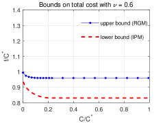
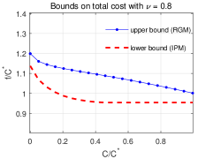
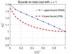
We plot in Fig. 1 both the upper bound $f_{U}(C)$ and the lower bound $f_{L}(C)$ of the optimal value of problem in (29) as a function of $C$ over the interval $[0,0.99C^{*}]$. There are several observations we make from the plots.

o1. When $\nu=0.6$ and the infection costs $\mathbf{c}$ are small, the left plot shows $f_{U}(C)<C^{*}$, which tells us that the local minimizer found by the projected RGM of the problem in (29) with the given security budget $C$, is better than the optimal point of (33). The plot also indicates that both the upper and lower bounds quickly reach a plateau less than $C^{*}$ with increasing $C$. This likely suggests that the optimal security investment at an optimal point of (28) is significantly smaller than $C^{*}$.

o2. As we discussed just before subsection 6.2.1, the left plot highlights the practical usefulness of our approach: by considering the problem in (29) for $C=C^{*}-\epsilon$ with small positive $\epsilon$, we can quickly estimate the optimal security investments, i.e., whether or not they are close to $C^{*}$ (when the security budget constraint is active at $\mathbf{s}^{*}_{C}$) or is equal to $w(\mathbf{s}^{*}_{C})$ (when the constraint is inactive at $\mathbf{s}^{*}_{C}$), without suffering from the numerical issues mentioned earlier.

o3. As $\nu$ increases, so do the bounds $f_{U}(C_{1})$ and $f_{L}(C_{1})$ (normalized by $C^{*}$). For larger values of $\nu$ with higher infection costs (middle and right plots), the upper bound $f_{U}(C_{1})$ obtained from a local minimizer is slightly larger than another upper bound $C^{*}$, suggesting that the budget constraint is active at a local minimizer returned by the projected RGM. This suggests that, when infection costs are high, $\mathbf{s}_{0}$, which may overinvest compared to an optimal point, may still be a good feasible point. Furthermore, as $\nu$ gets close to one, eventually $\mathbf{s}_{0}$ becomes an optimal point for the problem in (28) as shown in the right plot for $\nu=1$. This is expected because as the infection costs become larger, the system operator has an incentive to invest more in security.

o4. Although we do not report detailed numbers here, both the upper and lower bounds can be computed efficiently using RGM and MOSEK; the required computational time is always less than 2 seconds for each run, suggesting that the RGM may be a good method for identifying suitable security investments for large systems.

8 Discussion

8.1 Constraints on Security Investments

As mentioned in Section 3, we imposed only non-negativity constraints on security investments $\mathbf{s}$ in problem (P) and subsequent problems. In this subsection, we discuss how additional constraint(s) on $\mathbf{s}$, such as a budget constraint, affect our main results reported in Sections 4 through 6.

8.1.1 Case with $\boldsymbol{\lambda}\gneq\mathbf{0}$

Suppose that the security investments $\mathbf{s}$ is required to lie in some convex set ${\mathcal{S}}\subset\mathbb{R}_{+}^{N}$ in problem (P). Then, the relaxed problems ${\rm(P_{R1})}$ and ${\rm(P_{R2})}$ are still convex. However, the pair $(\tilde{\mathbf{s}},\tilde{\mathbf{p}})$ (resp. $(\mathbf{s}^{\prime},\mathbf{p}^{\prime})$) in Theorem 2 (resp. 3) is a feasible point of problem (P) if and only if $\tilde{\mathbf{s}}\in{\mathcal{S}}$ (resp. $\mathbf{s}^{\prime}\in{\mathcal{S}}$). For this reason, the convex relaxations ${\rm(P_{R1})}$ and ${\rm(P_{R2})}$ are exact if $\tilde{\mathbf{s}}$ and $\mathbf{s}^{\prime}$ lie in ${\mathcal{S}}$ and the condition (11) in Lemma 3 holds. In addition, in order to ensure that $\mathbf{s}^{(t+1)}$ belongs to ${\mathcal{S}}$, line 6 of Algorithm 2 needs to be modified as follows:

$$\mathbf{s}^{(t+1)}\leftarrow{\mathcal{P}}_{{\mathcal{S}}}\big{[}\mathbf{s}^{(t)}-\gamma_{t}\big{(}\nabla w(\mathbf{s}^{(t)})-\boldsymbol{\alpha}\circ\mathbf{p}^{(t)}\circ\mathbf{u}\big{)}\big{]},$$

where ${\mathcal{P}}_{{\mathcal{S}}}[\cdot]$ denotes the projection operator onto ${\mathcal{S}}$.

8.1.2 Case with $\boldsymbol{\lambda}=\mathbf{0}$

The finding in Theorem 5 continues to hold when the minimum element $\mathbf{s}_{\min}$ of the set ${\mathcal{S}}$ exists, with the minimum element $\mathbf{s}_{\min}$ being the unique optimal point of the problem in (28) when $\rho\big{(}\mathtt{diag}(\boldsymbol{\alpha}\circ\mathbf{s}_{\min}+\boldsymbol{\delta})^{-1}B\big{)}\leq 1$. Hence, when the recovery rates $\boldsymbol{\delta}$ are sufficiently large, only the minimum investments given by $\mathbf{s}_{\min}$ are needed. Obviously, when ${\mathcal{S}}=\mathbb{R}_{+}^{N}$, the minimum element is $\mathbf{0}$. Also, for a general constraint set ${\cal S}$, the problem in (33) is not guaranteed to be feasible, i.e., $\rho(\mathtt{diag}(\boldsymbol{\alpha}\circ\mathbf{s}+\boldsymbol{\delta})^{-1}B)>1$ for all $\mathbf{s}\in{\mathcal{S}}$. This means that $\mathbf{p}_{\rm se}(\mathbf{s})>\mathbf{0}$ for all $\mathbf{s}\in{\cal S}$ and our methods in Sections 4 and 5 can be applied directly to the problem in (28).

8.2 Relaxation of Irreducibility of $B$

Although we suspect that irreducibility of matrix $B$ is a reasonable assumption for many systems of interest, such as enterprise intranets, some systems may not satisfy this assumption. For this reason, here we discuss how relaxing this assumption affects our results.

Note that the irreducibility of $B$ is used to (i) ensure the existence of a unique equilibrium $\mathbf{p}^{*}(\mathbf{s})\in(0,1)^{N}$ of (1) as shown in Theorem 1, and (ii) make use of Lemma 2 for our M-matrix based convex formulations.

We relax the assumption that $B$ is irreducible and instead assume that, for every system $i\in{\mathcal{A}}$, either $\lambda_{i}>0$ or there is another system $j\in{\mathcal{A}}\setminus\{i\}$ with $\lambda_{j}>0$ and a directed path to $i$ in ${\cal G}$. Then, the main results in Theorem 1 still hold, i.e., there is a unique equilibrium $\mathbf{p}^{*}(\mathbf{s})\in(0,1)^{N}$ of (1) which is strictly positive and can be computed via iteration (2). Moreover, our formulations and results based on exponential cones, including the convex relaxation ${\rm(P_{R2})}$ and Theorem 3, are still valid because they rely only on the positivity of $\mathbf{p}(\mathbf{s})$. However, the convexity of problem ${\rm(P_{R1})}$ is not guaranteed and requires extending Lemma 2. Finally, when the aforementioned assumption does not hold, the problem is more complicated; our results cannot be applied directly, and it is still an open problem.

9 Conclusions

We studied the problem of determining suitable security investments for hardening interdependent component systems of large systems against malicious attacks and infections. Our formulation aims to minimize the average aggregate costs of a system operator based on the steady-state analysis. We showed that the resulting optimization problem is nonconvex, and proposed a set of algorithms for finding a good solution; two approaches are based on convex relaxations, and the other two look for a local minimizer based on RGM and SCP. In addition, we derived a sufficient condition under which the convex relaxations are exact. Finally, we evaluated the proposed algorithms and demonstrated that, although the original problem is nonconvex, local minimizers found by the RGM and SCP methods are good solutions with only small optimality gaps. In addition, as predicted by our analytical results, when the infection costs are high, the optimal points of convex relaxations solve the original nonconvex problem.

Van Sy Mai received his B.E. degree in Electrical Engineering from the Hanoi University of Technology in 2008, his M.E. degree in Electrical Engineering from the Chulalongkorn University in 2010, and his Ph.D. degree in Electrical and Computer Engineering from the University of Maryland in 2017. Since 2017, he has been a guest researcher at the National Institute of Standards and Technology.

Richard J. La received his Ph.D. degree in Electrical Engineering from the University of California, Berkeley in 2000. Since 2001 he has been on the faculty of the Department of Electrical and Computer Engineering at the University of Maryland, where he is currently a Professor. He is currently an associate editor for IEEE/ACM Transactions on Networking, and served as an associate editor for IEEE Transactions on Information Theory and IEEE Transactions on Mobile Computing.

Abdella Battou is the Division Chief of the Advanced Network Technologies Division, within The Information Technology Lab at NIST. He also leads the Cloud Computing Program. His research areas in Information and Communications Technology (ICT) include cloud computing, high performance optical networking, information centric networking, and more recently quantum networking. From 2009 to 2012, prior to joining NIST, he served as the Executive Director of The Mid-Atlantic Crossroads (MAX) GigaPop. From 2000 to 2009, he was Chief Technology Officer, and Vice President of Research and Development for Lambda OpticalSystems. Dr. Battou holds a PhD and MSEE in Electrical Engineering, and MA in Mathematics all from the Catholic University of America.

Appendix A Proof of Theorem 1

The existence and uniqueness of an equilibrium can be established following the same approach in [18], and we omit its proof here.

We now show that $\mathbf{p}^{*}$ can be obtained using the iteration in (2) of the theorem. Given $\boldsymbol{\lambda}\gneq\mathbf{0}$, $\boldsymbol{\delta},\mathbf{s}\geq\mathbf{0}$, it follows that the steady state $\mathbf{p}^{*}$ satisfies (5), which can be rewritten as

$$(\mathbf{1}-\mathbf{p}^{*})\circ(\boldsymbol{\lambda}+B\mathbf{p}^{*})=\mathbf{u}\circ\mathbf{p}^{*}$$ (40)

with $\mathbf{u}=\boldsymbol{\alpha}\circ\mathbf{s}+\boldsymbol{\delta}$. This is equivalent to

$$\mathbf{p}^{*}=\frac{\boldsymbol{\lambda}+B\mathbf{p}^{*}}{\boldsymbol{\lambda}+B\mathbf{p}^{*}+\mathbf{u}}=:H(\mathbf{p}^{*}).$$ (41)

This suggests that $\mathbf{p}^{*}$ is a fixed point of the map $H$. It can be verified that $H$ satisfies the following properties of a standard interference function [41]: for any $\mathbf{p}\geq\mathbf{p}^{\prime}\geq\mathbf{0}$, (i) $H(\mathbf{p})>\mathbf{0}$, (ii) $H(\mathbf{p})\geq H(\mathbf{p}^{\prime})$, and (iii) $cH(\mathbf{p})>H(c\mathbf{p})$ for $c>1$. As a result, the unique fixed point of $H$ can be computed using the iteration

$$\mathbf{p}_{k+1}=H(\mathbf{p}_{k})$$ (42)

starting from any $\mathbf{p}_{0}\geq\mathbf{0}$. The convergence of the synchronous version (as well as asynchronous one) can be found in [41]. However, little is known about the convergence rate except for when a stronger condition than (iii) is used. For example, linear convergence is achieved when $H$ is a contraction [9]. Here, we demonstrate linear convergence using a different, more direct argument.

First, for any $\mathbf{p}\geq\mathbf{p}^{\prime}\geq\mathbf{p}^{*}$, we have

$$\mathbf{0}\leq H(\mathbf{p})-H(\mathbf{p}^{\prime}) =\frac{\mathbf{u}\circ B(\mathbf{p}-\mathbf{p}^{\prime})}{(\mathbf{u}+\boldsymbol{\lambda}+B\mathbf{p})\circ(\mathbf{u}+\boldsymbol{\lambda}+B\mathbf{p}^{\prime})}$$

$$\leq\frac{\mathbf{u}\circ B(\mathbf{p}-\mathbf{p}^{\prime})}{(\mathbf{u}+\boldsymbol{\lambda}+B\mathbf{p}^{*})^{2}}$$

$$=\frac{(\mathbf{1}-\mathbf{p}^{*})^{2}}{\mathbf{u}}\circ B(\mathbf{p}-\mathbf{p}^{\prime})$$

$$=\mathtt{diag}(1-\mathbf{p}^{*})\Xi B(\mathbf{p}-\mathbf{p}^{\prime}),$$

where $\Xi=\mathtt{diag}(\frac{\mathbf{1}-\mathbf{p}^{*}}{\mathbf{u}})$, and the second equality is a consequence of $\mathbf{1}-\mathbf{p}^{*}=\frac{\mathbf{u}}{\mathbf{u}+\boldsymbol{\lambda}+B\mathbf{p}^{*}}$ from (41). Here, for a vector ${\bf x}$, we use ${\bf x}^{2}={\bf x}\circ{\bf x}$.

Next, we show that $\rho(\Xi B)\leq 1$, which then implies

$$\rho_{0}:=\rho\big{(}\mathtt{diag}(\mathbf{1}-\mathbf{p}^{*})\Xi B\big{)}\leq 1-\textstyle\min_{i}p_{i}^{*}<1.$$ (43)

To this end, note $\rho(\Xi B)\leq\rho\Big{(}\Xi\big{(}\mathtt{diag}(\frac{\boldsymbol{\lambda}}{\mathbf{p}^{*}})+B\big{)}\Big{)}=1$, where the inequality follows from the monotonicity of the spectral radius of nonnegative matrices [13, Thm 8.1.18], and the equality from the fact that $\mathbf{p}^{*}$ is a strictly positive eigenvector of $\Xi\big{(}\mathtt{diag}(\frac{\boldsymbol{\lambda}}{\mathbf{p}^{*}})+B\big{)}$ corresponding to eigenvalue $1$, i.e.,

$$\Xi\Big{(}\mathtt{diag}(\frac{\boldsymbol{\lambda}}{\mathbf{p}^{*}})+B\Big{)}\mathbf{p}^{*}=\Xi(\boldsymbol{\lambda}+B\mathbf{p}^{*})\stackrel{{\scriptstyle\eqref{eqSteadyState3}}}{{=}}\mathbf{p}^{*}.$$

Thus, we conclude that, starting from any $\mathbf{p}_{0}$ such that $\mathbf{p}^{*}\leq\mathbf{p}_{0}\leq\mathbf{1}$, $H$ is contractive with parameter $\rho_{0}<1$ given in (43). In fact, iteration (42) satisfies $0\leq\mathbf{p}_{k}-\mathbf{p}^{*}\leq\rho_{0}^{k}(\mathbf{p}_{0}-\mathbf{p}^{*})$, and linear convergence is achieved.

Appendix B A Proof of Convexity of $\Omega$

We will prove this convexity claim by using the convexity of the dominant eigenvalue of an essentially nonnegative matrix (also known as a Metzler matrix, i.e., off-diagonal elements are nonnegative). In particular, it is known that any Metzler matrix $A\in\mathbb{R}^{n\times n}$ has an eigenvalue $\bar{\sigma}(A)$ called the dominant eigenvalue that is real and greater than or equal to the real part of any other eigenvalue of $A$. The following result was shown in [6].

Theorem [6]: Let $A$ be a Metzler matrix and $D$ be a diagonal matrix. Then $\bar{\sigma}(A+D)$ is a convex function of $D$.

This theorem implies that $\underline{\sigma}(\mathtt{diag}(\mathbf{z})-B)$ is concave in $\mathbf{z}$.

Fix $\mathbf{z}_{1},\mathbf{z}_{2}\in\Omega$ and let $\mathbf{z}(\tau):=\tau\mathbf{z}_{1}+(1-\tau)\mathbf{z}_{2}$, $\tau\in[0,1]$. We will show that $\mathbf{z}(\tau)\in\Omega$ for all $\tau\in[0,1]$, which proves the convexity of $\Omega$. Becase $B$ is a Metzler matrix, from Lemma 1-(e)), the following equivalence holds: $\mathbf{z}\in\Omega$ if and only if $\underline{\sigma}(\mathtt{diag}(\mathbf{z})-B)>0$. Since $\mathbf{z}_{1},\mathbf{z}_{2}\in\Omega$, we have $\underline{\sigma}(\mathtt{diag}(\mathbf{z}_{i})-B)>0$ for $i=1,2$. This, together with the concavity of $\underline{\sigma}(\mathtt{diag}(\mathbf{z})-B)$, gives us the inequality

$$\underline{\sigma}(\mathtt{diag}(\mathbf{z}(\tau))-B)$$

$$\geq \tau\underline{\sigma}(\mathtt{diag}(\mathbf{z}_{1})-B)+(1-\tau)\underline{\sigma}(\mathtt{diag}(\mathbf{z}_{2})-B)$$

which is strictly positive for all $\tau\in[0,1]$.

Appendix C Formulation of (12) as a Matrix Balancing Problem

First, recall that a matrix $A\in\mathbb{R}^{n\times n}_{+}$ is balanced if $A\mathbf{1}=A^{\mathsf{T}}\mathbf{1}$. A positive diagonal matrix $X$ is said to balance a matrix $A\in\mathbb{R}^{n\times n}_{+}$ if $XAX^{-1}$ is balanced. The following lemma holds [39]:

Lemma 6.

For any $A\in\mathbb{R}^{n\times n}_{+}$, let $\mathcal{G}_{A}$ denote the weighted directed graph associated with $A$. Then, the following statements are equivalent:

• A positive diagonal matrix $X$ that balances $A$ exists.

• The graph $\mathcal{G}_{A}$ is strongly connected.

• There exists a positive vector ${\mathbf{x}}$ that minimizes the sum $\sum_{1\leq i,j\leq n}a_{ij}x_{i}x_{j}^{-1}$.

Moreover, matrix $X$ and vector ${\mathbf{x}}$ are unique up to scalars.

We now proceed to prove that (12) is a matrix balancing problem. Suppose that $\underline{\sigma}(\mathtt{diag}(\mathbf{z})-B)=0$, which is equivalent to the condition that $\mathtt{diag}(\mathbf{z})-B$ is a singular M-matrix (i.e., $\mathbf{z}\in\partial\Omega$). Then, there exists $\tilde{B}\in\mathbb{R}^{N\times N}_{+}$ such that $\mathtt{diag}(\mathbf{z})-B=\rho(\tilde{B})I-\tilde{B}.$ Since $\tilde{B}$ is also irreducible, it follows from the Perron-Frobenius theorem [13] that there is ${\mathbf{x}}>\mathbf{0}$ such that $\tilde{B}{\mathbf{x}}=\rho(\tilde{B}){\mathbf{x}}$. As a result, $(\mathtt{diag}(\mathbf{z})-B){\mathbf{x}}=\mathbf{0}$, i.e.,

$$\textstyle\sum_{j=1}^{N}b_{ij}x_{j}x_{i}^{-1}=z_{i},\quad\forall i=1,\ldots,n.$$ (44)

Therefore, we can write (12) as follows.

$$\textstyle\min_{\mathbf{z}>\mathbf{0}}\quad\{\mathbf{h}^{\mathsf{T}}\mathbf{z}~{}|~{}\underline{\sigma}\big{(}\mathtt{diag}(\mathbf{z})-B\big{)}=0\}$$

$$= \textstyle\min_{\mathbf{z}>\mathbf{0},{\mathbf{x}}>\mathbf{0}}\quad\{\mathbf{h}^{\mathsf{T}}\mathbf{z}~{}|~{}\eqref{eqEigvec}\text{ holds}\}$$

$$= \textstyle\min_{{\mathbf{x}}>\mathbf{0}}\quad\sum_{1\leq i,j\leq n}h_{i}b_{ij}x_{j}x_{i}^{-1}$$

which, by Lemma 6, is the problem of balancing $\mathtt{diag}(\mathbf{h})B$.

Appendix D A Proof of Theorem 3

The first inequality in (17) is obvious because $({\rm P_{R2}})$ is a relaxation of $({\rm P})$. The second inequality follows from the feasibility of $(\mathbf{s}^{\prime},\mathbf{p}^{\prime})$ as shown below.

D.1 Proof of Feasibility of $(\mathbf{s}^{\prime},\mathbf{p}^{\prime})$ for (P)

Recall that

$$\mathbf{p}^{\prime}=e^{-\mathbf{y}^{+}}>\mathbf{0}\quad\mathbf{s}^{\prime}=\mathbf{s}^{+}+\mathtt{diag}(\boldsymbol{\alpha}^{-1})B(\mathbf{p}^{+}-\mathbf{p}^{\prime}).$$

Since $\mathbf{s}^{+}\geq\mathbf{0}$ and $\mathbf{p}^{+}\geq e^{-\mathbf{y}^{+}}=\mathbf{p}^{\prime}$, it follows that $\mathbf{s}^{\prime}\geq\mathbf{0}$. It remains to show that $(\mathbf{s}^{\prime},\mathbf{p}^{\prime})$ satisfies the constraint (4b) or, equivalently,

$$(\mathbf{p}^{\prime})^{-1}\circ\boldsymbol{\lambda}+(\mathbf{p}^{\prime})^{-1}\circ B\mathbf{p}^{\prime}=\boldsymbol{\lambda}+B\mathbf{p}^{\prime}+\boldsymbol{\alpha}\circ\mathbf{s}^{\prime}+\boldsymbol{\delta}.$$ (5)

From the definition of $(\mathbf{p}^{\prime},\mathbf{s}^{\prime})$, (5) is equivalent to

$$e^{\mathbf{y}^{+}}\circ\boldsymbol{\lambda}+e^{\mathbf{y}^{+}}\circ Be^{-\mathbf{y}^{+}}=\boldsymbol{\lambda}+B\mathbf{p}^{+}+\boldsymbol{\alpha}\circ\mathbf{s}^{+}+\boldsymbol{\delta},$$

where the right-hand side equals $\mathbf{t}^{+}+U^{+}\mathbf{1}$ from (14).

To show that the above equality holds, we will prove that the equalities

$$\mathbf{t}^{+}=\boldsymbol{\lambda}\circ e^{\mathbf{y}^{+}},\quad U^{+}=\mathtt{diag}(e^{\mathbf{y}^{+}})B\mathtt{diag}(e^{-\mathbf{y}^{+}})$$ (18)

hold, i.e., the inequality constraints of $\mathbf{t}$ and $U$ are active at the solution ${\bf x}^{+}_{\rm R}$ of problem $({\rm P_{R2}})$. Let $\boldsymbol{\mu}_{s}$, $\boldsymbol{\mu}_{p},\overline{\boldsymbol{\mu}}_{p}$, $\boldsymbol{\mu}_{t}$, $\boldsymbol{\mu}_{y}\in\mathbb{R}^{N}_{+}$ and $\Phi\in\mathbb{R}^{N\times N}_{+}$ be the Lagrangian multipliers associated with inequality constraints, and $\boldsymbol{\sigma}\in\mathbb{R}^{N}$ with the equality constraint in (14) of $({\rm P_{R2}})$. Then, the Lagrangian function is given by

$$L= w(\mathbf{s})+\langle\mathbf{c},\mathbf{p}\rangle+\langle\boldsymbol{\mu}_{p},e^{-\mathbf{y}}-\mathbf{p}\rangle+\langle\boldsymbol{\mu}_{t},\boldsymbol{\lambda}\circ e^{\mathbf{y}}-\mathbf{t}\rangle$$

$$+\langle\Phi,\mathtt{diag}(e^{\mathbf{y}})B\mathtt{diag}(e^{-\mathbf{y}})-U\rangle$$

$$-\langle\boldsymbol{\mu}_{s},\mathbf{s}\rangle+\langle\overline{\boldsymbol{\mu}}_{p},\mathbf{p}-\mathbf{1}\rangle-\langle\boldsymbol{\mu}_{y},\mathbf{y}\rangle$$

$$+\langle\boldsymbol{\sigma},\mathbf{t}+U\mathbf{1}-\boldsymbol{\lambda}-B\mathbf{p}-\boldsymbol{\alpha}\circ\mathbf{s}-\boldsymbol{\delta}\rangle.$$

Since the problem is convex, the following Karush-Kuhn-Tucker (KKT) conditions are necessary and sufficient for optimality.

$$\mathbf{0} = \nabla_{p}L=\mathbf{c}-\boldsymbol{\mu}_{p}+\overline{\boldsymbol{\mu}}_{p}-B^{\mathsf{T}}\boldsymbol{\sigma}$$ (45a)

$$\mathbf{0} = \nabla_{t}L=\boldsymbol{\sigma}-\boldsymbol{\mu}_{t}$$ (45b)

$$0 = \partial_{u_{ij}}L=\sigma_{i}-\phi_{ij}\ \mbox{ for all }(i,j)\in\mathcal{E}$$ (45c)

$$0 = \partial_{y_{i}}L=\mu_{t_{i}}\lambda_{i}e^{y_{i}^{+}}-\mu_{p_{i}}e^{-y_{i}^{+}}-\mu_{y_{i}}+\sum_{j\in\mathcal{A}}\phi_{ij}b_{ij}e^{y_{i}^{+}\!-y_{j}^{+}}$$ (45d)

$$\qquad-\sum_{j\in\mathcal{A}}\phi_{ji}b_{ji}e^{y^{+}_{j}\!-y^{+}_{i}}\ \mbox{ for all }i\in\mathcal{A}$$

$$\mathbf{0} = \boldsymbol{\mu}_{t}\circ(e^{\mathbf{y}^{+}}-\mathbf{t}^{+})$$ (45e)

$$0 = \phi_{ij}(u^{+}_{ij}-b_{ij}e^{y^{+}_{i}-y^{+}_{j}})\ \mbox{ for all }(i,j)\in\mathcal{E}.$$ (45f)

From (45b) and (45c), we get

$$\sigma_{i}=\mu_{t_{i}}=\phi_{ij}\geq 0\ \mbox{ for all }(i,j)\in\mathcal{E}.$$ (46)

Combining this and (45d) yields

$$\sigma_{i}(\lambda_{i}e^{y_{i}^{+}}+\sum_{j}b_{ij}e^{y_{i}^{+}-y_{j}^{+}})$$

$$= \mu_{p_{i}}e^{-y_{i}^{+}}\!+\!\mu_{y_{i}}+\sum_{j}\sigma_{j}b_{ji}e^{y_{j}^{+}-y_{i}^{+}}$$

$$\geq (\mu_{p_{i}}+\sum_{j}\sigma_{i}b_{ji})e^{-y_{i}^{+}}\geq(c_{i}+\overline{\mu}_{p_{i}})e^{-y_{i}^{+}}>0,$$

where the first inequality follows from $\boldsymbol{\mu}_{y}\geq\mathbf{0}$ and $\mathbf{y}^{+}\geq\mathbf{0}$, and the second from (45a). Thus, $\boldsymbol{\sigma}>\mathbf{0}$, which together with (46) and the slackness conditions (45e) and (45f) implies that (18) must hold.

D.2 Equivalence of Relaxed Problems $({\rm P_{R1}})$ and $({\rm P_{R2}})$

We will show that $({\rm P_{R1}})$ and $({\rm P_{R2}})$ are equivalent. Recall

$$(\mathrm{P_{R1}})\qquad\min_{\mathbf{s},\mathbf{p},\mathbf{z}} f(\mathbf{s},\mathbf{p})$$

$$\mathsf{s.t.} \mathbf{p}\geq(\mathtt{diag}(\mathbf{z})-B)^{-1}\boldsymbol{\lambda}$$

$$\mathbf{z}=\boldsymbol{\alpha}\circ\mathbf{s}+\boldsymbol{\delta}+\boldsymbol{\lambda}+B\mathbf{p}$$

$$\mathbf{s}\geq\mathbf{0},\quad\mathbf{p}\leq\mathbf{1},\quad\mathbf{z}\in\Omega.$$

Let $\mathbf{v}:=(\mathtt{diag}(\mathbf{z})-B)^{-1}\boldsymbol{\lambda}$. Then, we have

$$(\mathtt{diag}(\mathbf{z})-B)\mathbf{v}=\boldsymbol{\lambda}.$$ (48)

Since $B$ is irreducible, Lemma 1-(f) implies that if $\mathbf{v}>\mathbf{0}$, we have $\mathbf{z}\in\Omega$ because $\boldsymbol{\lambda}\gneq\mathbf{0}$. In addition, we can show that if $\mathbf{z}\in\Omega$, then $(\mathtt{diag}(\mathbf{z})-B)^{-1}>0$ and thus $\mathbf{v}>\mathbf{0}$. Thus, $\mathbf{z}\in\Omega$ if and only if $\mathbf{v}>\mathbf{0}$ and, when $\mathbf{v}>\mathbf{0}$, (48) is equivalent to

$$\mathtt{diag}(\mathbf{v}^{-1})(\mathtt{diag}(\mathbf{z})-B)\mathbf{v}=\mathtt{diag}(\mathbf{v}^{-1})\boldsymbol{\lambda}.$$

Rearranging the terms, we get

$$\mathbf{z}=\mathbf{v}^{-1}\circ B\mathbf{v}+\mathbf{v}^{-1}\circ\boldsymbol{\lambda}.$$ (49)

Substituting the expressions for $\mathbf{v}$ and $\mathbf{z}$ in the first and second constraint, respectively, and replacing the constraint $\mathbf{z}\in\Omega$ with $\mathbf{v}>\mathbf{0}$, we can reformulate $(\mathrm{P_{R1}})$ as follows.

$$\min_{\mathbf{s},\mathbf{p},\mathbf{v}} f(\mathbf{s},\mathbf{p})$$ (50)

$$\mathsf{s.t.} \mathbf{p}\geq\mathbf{v}$$

$$\mathbf{v}^{-1}\circ B\mathbf{v}+\mathbf{v}^{-1}\circ\boldsymbol{\lambda}=\boldsymbol{\alpha}\circ\mathbf{s}+\boldsymbol{\delta}+\boldsymbol{\lambda}+B\mathbf{p}$$

$$\mathbf{s}\geq\mathbf{0},\quad\mathbf{p}\leq\mathbf{1},\quad\mathbf{v}>\mathbf{0}.$$

Next, we will show that this problem is equivalent to $(\mathrm{P_{R2}})$. Recall that, as we showed in the previous subsection, at any optimal point ${\bf x}^{+}=(\mathbf{s}^{+},\mathbf{p}^{+},\mathbf{y}^{+},\mathbf{t}^{+},U^{+})$ of $(\mathrm{P_{R2}})$, equalities in (18) hold. Thus, $(\mathrm{P_{R2}})$ can be reduced to the following problem after eliminating $\mathbf{t}$ and $U$.

$$\min_{\mathbf{s},\mathbf{p},\mathbf{y}} \quad f(\mathbf{s},\mathbf{p})$$ (51)

$$\mathsf{s.t.} \quad\mathbf{p}\geq e^{-\mathbf{y}}$$

$$\quad\boldsymbol{\lambda}\circ e^{\mathbf{y}}+e^{\mathbf{y}}\circ Be^{-\mathbf{y}}=\boldsymbol{\alpha}\circ\mathbf{s}\!+\!\boldsymbol{\delta}\!+\!\boldsymbol{\lambda}\!+\!B\mathbf{p}$$

$$\quad\mathbf{s}\geq\mathbf{0},\quad\mathbf{p}\leq\mathbf{1},\quad\mathbf{y}\geq\mathbf{0}.$$

Clearly, (51) is identical to (50) after replacing $e^{-\mathbf{y}}$ with $\mathbf{v}$. This proves the equivalence of $({\rm P_{R1}})$ and $({\rm P_{R2}})$.

Appendix E A Proof of Theorem 4

In order to prove the theorem, it suffices to show that at any optimal point ${\bf x}^{+}=(\mathbf{s}^{+},\mathbf{y}^{+},\mathbf{t}^{+},U^{+})$ of the relaxed problem in (27), the constraints (27b) and (27c) are active. In other words,

$$\mathbf{t}^{+}=\boldsymbol{\lambda}\circ e^{\mathbf{y}^{+}},\quad U^{+}=\mathtt{diag}(e^{\mathbf{y}^{+}})B\mathtt{diag}(e^{-\mathbf{y}^{+}}).$$ (52)

The proof is similar to that in Appendix D. Let $\boldsymbol{\mu}_{s}$, $\boldsymbol{\mu}_{t}\in\mathbb{R}^{N}_{+}$ and $\Phi\in\mathbb{R}^{N\times N}_{+}$ be the Lagrange multipliers associated with inequality constraints (27b) and (27c), and $\boldsymbol{\sigma}\in\mathbb{R}^{N}$ those associated with the equality constraint (27a) of the relaxed problem. The Lagrangian is given by

$$L =w(\mathbf{s})+\langle\mathbf{c},e^{-\mathbf{y}}\rangle-\langle\boldsymbol{\mu}_{s},\mathbf{s}\rangle+\langle\boldsymbol{\mu}_{t},\boldsymbol{\lambda}\circ e^{\mathbf{y}}-\mathbf{t}\rangle$$

$$\quad+\langle\Phi,\mathtt{diag}(e^{\mathbf{y}})B^{(t)}\mathtt{diag}(e^{-\mathbf{y}})-U\rangle$$

$$\quad+\langle\boldsymbol{\sigma},\mathbf{t}+U\mathbf{1}-\boldsymbol{\lambda}-B\mathbf{p}^{(t)}-\boldsymbol{\alpha}\circ\mathbf{s}-\boldsymbol{\delta}\rangle.$$ (53)

Since the problem is convex, the necessary and sufficient KKT conditions are given by the following:

$$\mathbf{0} = \nabla_{t}L=\boldsymbol{\sigma}-\boldsymbol{\mu}_{t}$$ (54a)

$$0 = \partial_{u_{ij}}L=\sigma_{i}-\phi_{ij}\ \mbox{ for all }(i,j)\in\mathcal{E}$$ (54b)

$$0 = \partial_{y_{i}}L=-c_{i}e^{-y_{i}^{+}}+\mu_{t_{i}}\lambda_{i}e^{y_{i}^{+}}+\sum_{j}\phi_{ij}b^{(t)}_{ij}e^{y_{i}^{+}-y_{j}^{+}}$$ (54c)

$$\qquad-\sum_{j}\phi_{ji}b^{(t)}_{ji}e^{y^{+}_{j}-y^{+}_{i}}\ \mbox{ for all }i\in\mathcal{A}$$

$$\mathbf{0} = \boldsymbol{\mu}_{t}\circ(e^{\mathbf{y}^{+}}-\mathbf{t}^{+})$$ (54d)

$$0 = \phi_{ij}(u^{+}_{ij}-b^{(t)}_{ij}e^{y^{+}_{i}-y^{+}_{j}})\ \mbox{ for all }(i,j)\in\mathcal{E}.$$ (54e)

From (54a) and (54b),

$$\sigma_{i}=\mu_{t_{i}}=\phi_{ij}\geq 0\ \mbox{ for all }(i,j)\in\mathcal{E}.$$ (55)

By combining this and (54c), we obtain

$$\sigma_{i}\big{[}\lambda_{i}e^{y_{i}^{+}}+\sum_{j}b^{(t)}_{ij}e^{y_{i}^{+}-y_{j}^{+}}\big{]}=c_{i}e^{-y_{i}^{+}}+\sum_{j}\sigma_{j}b^{(t)}_{ji}e^{y_{j}^{+}-y_{i}^{+}},$$

which is strictly positive because $c_{i}>0$. Thus, $\boldsymbol{\sigma}>\mathbf{0}$, which together with (55) and the slackness conditions in (54d) and (54e), implies that (52) must hold.

Appendix F Proof of Theorem 6

Suppose $(\mathbf{s}_{L},\mathbf{p}_{L},\mathbf{y}_{L},U_{L})$ is an optimal point of $({\rm P_{R3}})$, and let $C_{L}=w(\mathbf{s}_{L})$. There are two possibilities: $C_{L}=C$ or $C_{L}<C$. We shall consider them separately below.

$\bullet$ $C_{L}=C$: In this case, we have

$$C^{*}-\epsilon=w(\mathbf{s}_{L})<f_{L}(C),$$ (56)

where the inequality follows from the assumption $C<C^{*}$ and, hence, $\mathbf{p}_{\rm se}(\mathbf{s}_{L})>\mathbf{0}$. Since the relaxed problem $({\rm P_{R3}}$) is convex, $f_{L}(C)$ is a convex function of $C$ [5]. Thus, we have

$$f_{L}(C)\leq\big{(}1-\frac{\epsilon}{C^{*}}\big{)}f_{L}^{*}+\frac{\epsilon}{C^{*}}f_{L}(0)\stackrel{{\scriptstyle\eqref{eqFLstar}}}{{\leq}}f_{0}^{*}+\frac{\epsilon}{C^{*}}\big{(}f_{L}(0)-f_{L}^{*}\big{)}.$$

Combining this with (56) yields

$$0\stackrel{{\scriptstyle\eqref{eq:w*1}}}{{\leq}}C^{*}-f_{0}^{*}\leq\epsilon+\frac{\epsilon}{C^{*}}\big{(}f_{L}(0)-f_{L}^{*}\big{)}.$$ (57)

Suppose that $\mathbf{s}_{0}$ is an optimal point of (33). Then, (57) implies that $\mathbf{s}_{0}$ is $O(\epsilon)$-suboptimal for the original problem in (28).

$\bullet$ $C_{L}<C$: Since the constraint $w(\mathbf{s}_{L})\leq C$ is inactive, it follows that $f_{L}(C_{L})=f_{L}(C^{\prime})$ for all $C^{\prime}\in[C_{L},C]$. Because $C$ can be made arbitrarily close to $C^{*}$, this also tells us that $f_{L}(C_{L})=f^{*}_{L}$, providing us with a following lower bound: $f_{L}^{*}=f_{L}(C_{L})\leq f_{0}^{*}$. This lower bound, together with an upper bound we can obtain as explained in subsection 6.2.2, can be used to quantify how close to optimal a feasible solution is.

Appendix G A Proof of Theorem 7

We prove the first part by contradiction: suppose that there exists some $C<C^{*}$ such that, at an optimal point $(\mathbf{s}_{L},\mathbf{p}_{L},\mathbf{y}_{L},U_{L})$, we have $C_{L}<C$. Consider

$$\mathbf{y}^{\prime}=\mathbf{y}_{L}+\gamma\mathbf{1},\ \ \mathbf{p}^{\prime}=e^{-\gamma}\mathbf{p}_{L},\ \ \mathbf{s}^{\prime}=\mathbf{s}_{L}+(1-e^{-\gamma})\boldsymbol{\alpha}^{-1}\circ B\mathbf{p}_{L}$$

for some $\gamma>0$ such that $w(\mathbf{s}^{\prime})<C$. We can find such positive $\gamma$ because $w$ is continuous and increasing, and $w(\mathbf{s}_{L})=C_{L}<C$. We can verify that the tuple $(\mathbf{s}^{\prime},\mathbf{p}^{\prime},\mathbf{y}^{\prime},U_{L})$ is a feasible point of the relaxed problem $({\rm P_{R3}})$. Moreover,

$$f(\mathbf{s}^{\prime},\mathbf{p}^{\prime})-f(\mathbf{s}_{L},\mathbf{p}_{L})=w(\mathbf{s}^{\prime})-w(\mathbf{s}_{L})+\mathbf{c}^{\mathsf{T}}(\mathbf{p}^{\prime}-\mathbf{p}_{L})$$

$$\leq\nabla w(\mathbf{s}^{\prime})^{\mathsf{T}}(\mathbf{s}^{\prime}-\mathbf{s}_{L})+(e^{-\gamma}-1)\mathbf{c}^{\mathsf{T}}\mathbf{p}_{L}$$

$$=(1-e^{-\gamma})\big{(}B^{\mathsf{T}}\mathtt{diag}(\boldsymbol{\alpha}^{-1})\nabla w(\mathbf{s}^{\prime})-\mathbf{c}\big{)}^{\mathsf{T}}\mathbf{p}_{L}<0.$$

The second inequality holds because $\gamma>0$, $\mathbf{p}_{L}>\mathbf{0},\mathbf{s}^{\prime}\in\mathbb{S}_{C}$ and the condition (38) is true. But, this contradicts the assumed optimality of $(\mathbf{s}_{L},\mathbf{p}_{L},\mathbf{y}_{L},U_{L})$. Hence, we have $C_{L}=C$.

To prove the second part of theorem, assume that (38) holds for all $\mathbf{s}\in\mathbb{S}_{C^{*}}$. Take any sequence of positive $\epsilon_{k}$, $k\in{\mathbb{N}}$, which satisfies $\lim_{k\to\infty}\epsilon_{k}=0$, and consider the sequence $\{C_{k}=C^{*}-\epsilon_{k}:k\in{\mathbb{N}}\}$. Because $\mathbb{S}_{C_{k}}\subset\mathbb{S}_{C^{*}}$, from (37), we obtain

$$C^{*}-f^{*}_{0}\leq\epsilon_{k}+\frac{\epsilon_{k}}{C^{*}}\big{(}f_{L}(0)-f^{*}_{L}\big{)}\ \mbox{ for all }k\in{\mathbb{N}}.$$

Since the right-hand side goes to 0 as $k\to\infty$, $f_{0}^{*}=C^{*}$ and $\mathbf{s}_{0}$ is an optimal point of the original problem in (28).

Appendix H Reformulation of Problem (33) As a Convex (Exponential Cone) Problem

Recall that the optimization problem is given by

$$(\mathrm{P}_{C})\hskip 21.68121pt\min_{\mathbf{s}\in\mathbb{R}^{N}_{+}} w(\mathbf{s})$$

$$\mathsf{s.t.} \rho(\mathtt{diag}(\boldsymbol{\alpha}\circ\mathbf{s}+\boldsymbol{\delta})^{-1}B)\leq 1.$$

By Perron-Frobenius theory [13], the above spectral radius constraint is equivalent to the existence of a positive vector ${\bf x}$ such that $\mathtt{diag}(\boldsymbol{\alpha}\circ\mathbf{s}+\boldsymbol{\delta})^{-1}B{\bf x}\leq{\bf x}$. With a change of variable $\mathbf{y}=\log({\mathbf{x}})$, problem $(\mathrm{P}_{C})$ can be expressed as follows.

$$\min_{\mathbf{s}\geq\mathbf{0},{\bf y}} \quad w(\mathbf{s})$$ (58)

$$\mathsf{s.t.} \quad\textstyle\sum_{j\in\mathcal{A}}b_{ij}e^{y_{j}-y_{i}}\leq\alpha_{i}s_{i}+\delta_{i},\quad\forall i\in\mathcal{A}.$$ (59)

This is a convex problem and can be turned into an exponential cone optimization problem as follows with $U=[u_{ij}]\in\mathbb{R}^{N\times N}$:

$$\min_{\mathbf{s}\geq\mathbf{0},{\bf y},U} w(\mathbf{s})$$ (60)

$$\mathsf{s.t.} U\mathbf{1}\leq\boldsymbol{\alpha}\circ\mathbf{s}+\boldsymbol{\delta}$$

$$(u_{ij},1,y_{i}-y_{j}+\log b_{ij})\in\mathcal{K}_{\rm exp},\quad\forall(i,j)\in\mathcal{E}$$

This problem can be solved efficiently using convex solvers [1, 8], provided that $N$ is not large.

Below, we describe a first-order algorithm for solving the problem in (60) based on our previous matrix balancing algorithm. This algorithm can deal with large-scale problems in a parallel and distributed fashion. For our discussion, without loss of generality, we assume $\boldsymbol{\alpha}=\mathbf{1}$. Let us consider the Lagrangian given by

$$L(\mathbf{y},\mathbf{s},\boldsymbol{\theta}) =w(\mathbf{s})+\sum_{i\in\mathcal{V}}\theta_{i}\Big{(}\sum_{j\in\mathcal{V}}b_{i,j}e^{y_{j}-y_{i}}-s_{i}-\delta_{i}\Big{)}$$

$$=w(\mathbf{s})-\boldsymbol{\theta}^{\mathsf{T}}(\mathbf{s}+\boldsymbol{\delta})+\sum_{(i,j)\in\mathcal{E}}\theta_{i}b_{i,j}e^{y_{j}-y_{i}},$$ (61)

where $\boldsymbol{\theta}\geq 0$ is a Lagrange multiplier vector. The dual function can be obtained from the Lagrangian by solving the following problem:

$$g(\boldsymbol{\theta}) :=\inf_{\mathbf{y}\in\mathbb{R}^{N},\mathbf{s}\geq\mathbf{0}}L(\mathbf{y},\mathbf{s},\boldsymbol{\theta})$$

$$=\inf_{\mathbf{s}\geq\mathbf{0}}w(\mathbf{s})-\boldsymbol{\theta}^{\mathsf{T}}(\mathbf{s}+\boldsymbol{\delta})+\inf_{\mathbf{y}}\sum_{(i,j)\in\mathcal{E}}\theta_{i}b_{i,j}e^{y_{j}-y_{i}},$$

It is obvious that this problem can be decoupled into two subproblems -- one over $\mathbf{s}$ and the other over $\mathbf{y}$ -- as follows.

$$\mathbf{s}(\boldsymbol{\theta}) =\arg\inf_{\mathbf{s}\geq\mathbf{0}}w(\mathbf{s})-\boldsymbol{\theta}^{\mathsf{T}}\mathbf{s}$$

$$\mathbf{y}(\boldsymbol{\theta}) =\arg\inf_{\mathbf{y}}\sum_{i,j\in\mathcal{E}}\theta_{i}b_{i,j}e^{y_{j}-y_{i}}$$

Note that the second problem of finding $\mathbf{y}(\boldsymbol{\theta})$ is a problem of balancing the matrix $\mathtt{diag}(\boldsymbol{\theta})B$ and can be solved efficiently.

The dual function is now equal to

$$g(\boldsymbol{\theta})=w(\mathbf{s}(\boldsymbol{\theta}))\!-\!\boldsymbol{\theta}^{\mathsf{T}}(\mathbf{s}(\boldsymbol{\theta})+\boldsymbol{\delta})\!+\!\!\sum_{(i,j)\in\mathcal{E}}\theta_{i}b_{ij}e^{y_{j}(\boldsymbol{\theta})-y_{i}(\boldsymbol{\theta})},$$

and the dual problem given by

$$\max_{\boldsymbol{\theta}\geq\mathbf{0}}~{}~{}~{}g(\boldsymbol{\theta})$$

is a convex problem. Suppose that the Slater’s condition holds for problem (58) so that we have strong duality. Then, we can solve (58) by solving the dual problem instead, for example, using a first-order method with subgradients.

Appendix I A Proof of the continuity of Stable Equilibrium $\mathbf{p}_{\rm se}$

We will prove the claim by contradiction. Suppose that $\mathbf{p}_{\rm se}$ is not continuous at some point $\mathbf{s}^{\prime}\in\mathbb{R}^{N}_{+}$. Then, there exists a sequence $\mathbf{s}_{k}$, $k\in{\mathbb{N}}$, such that $\mathbf{s}_{k}\to\mathbf{s}^{\prime}$ as $k\to\infty$, but either (a) $\lim_{k\to\infty}\mathbf{p}_{\rm se}(\mathbf{s}_{k})$ does not exist or (b) the limit exists but is not equal to $\mathbf{p}_{\rm se}(\mathbf{s}^{\prime})$. When the limit does not exist, we can work with a convergent subsequence instead; the existence of a convergent subsequence of $\mathbf{p}_{\rm se}(\mathbf{s}_{k})$, $k\in{\mathbb{N}}$, is guaranteed by the Bolzano-Weierstrass Theorem [38]. For this reason, without loss of generality, we assume $\lim_{k\to\infty}\mathbf{p}_{\rm se}(\mathbf{s}_{k})$ exists and denote it by $\mathbf{p}^{\dagger}$.

We consider the following two cases separately. Note that $\mathbf{p}_{\rm se}(\mathbf{s})$ cannot have both positive and zero entries.

Case 1: $\mathbf{p}_{\rm se}(\mathbf{s}^{\prime})>{\bf 0}$ – Recall from subsection 3.2 that when $\boldsymbol{\lambda}=\mathbf{0}$,

$$\mathbf{g}(\mathbf{s},\mathbf{p})=({\bf 1}-\mathbf{p})\circ B\mathbf{p}-(\boldsymbol{\alpha}\circ\mathbf{s}+\boldsymbol{\delta})\circ\mathbf{p}.$$

Since $\mathbf{g}(\mathbf{s}^{\prime},\mathbf{p}_{\rm se}(\mathbf{s}^{\prime}))={\bf 0}$, the implicit function theorem [12, Theorem 3] tells us that, for any set $\mathbb{P}^{\prime}$ containing $\mathbf{p}_{\rm se}(\mathbf{s}^{\prime})$, we can find a set $\mathbb{S}^{\prime}$ containing $\mathbf{s}^{\prime}$ and a function $\psi:\mathbb{S}^{\prime}\to\mathbb{P}^{\prime}$ such that (a) $\psi(\mathbf{s}^{\prime})=\mathbf{p}_{\rm se}(\mathbf{s}^{\prime})$, (b) $\mathbf{g}(\mathbf{s},\psi(\mathbf{s}))={\bf 0}$ for all $\mathbf{s}\in\mathbb{S}^{\prime}$, and (c) $\psi$ is continuous at $\mathbf{s}^{\prime}$. Since there is at most one positive stable equilibrium satisfying $\mathbf{g}(\mathbf{s},\mathbf{p})={\bf 0}$, this implies $\psi(\mathbf{s})=\mathbf{p}_{\rm se}(\mathbf{s})>{\bf 0}$ for all $\mathbf{s}$ in a sufficiently small neighborhood around $\mathbf{s}^{\prime}$ and, hence, $\mathbf{p}^{\dagger}=\mathbf{p}_{\rm se}(\mathbf{s}^{\prime})$, which is a contradiction.

Case 2: $\mathbf{p}_{\rm se}(\mathbf{s}^{\prime})={\bf 0}$ – In this case, since there is a unique solution to $\mathbf{g}(\mathbf{s}^{\prime},\mathbf{p})={\bf 0}$, $\mathbf{p}^{\dagger}$ must be equal to ${\bf 0}$ from the continuity of $\mathbf{g}$, which contradicts the earlier assumption that $\mathbf{p}^{\dagger}\neq\mathbf{p}_{\rm se}(\mathbf{s}^{\prime})={\bf 0}$.

Appendix J A Description of the Setup for Numerical Studies

The setup for running our algorithms is as follows.

$\bullet$ M-matrix + OPTI : In line 3 of Algorithm 1 for solving $(\rm{P_{R1}})$ with $\Omega$ replaced by $\tilde{\Omega}(\mathbf{z}^{(t)})$, we use a general interior point optimizer from package [8] with relative convergence tolerance set to $10^{-5}$ and Hessian matrices approximated by a quasi-Newton algorithm. The solver initial point $\tilde{{\bf x}}_{\rm{R}}^{(0)}\!=\!(\tilde{\mathbf{s}}_{\rm{R}}^{(0)},\tilde{\mathbf{p}}_{\rm{R}}^{(0)},\tilde{\mathbf{z}}_{\rm{R}}^{(0)})$ is chosen to be $\tilde{\mathbf{s}}_{\rm{R}}^{(0)}\!=\!\mathbf{0}$, $\tilde{\mathbf{p}}_{\rm{R}}^{(0)}\!=\!\mathbf{p}^{*}(\mathbf{0})$ using the iteration in (2), and $\tilde{\mathbf{z}}_{\rm{R}}^{(0)}=\boldsymbol{\lambda}+\boldsymbol{\delta}+B\tilde{\mathbf{p}}_{\rm{R}}^{(0)}$ according to (7). When computing $\tilde{\mathbf{p}}_{\rm{R}}^{(0)}$, the iteration in (2) is run until either $\left|\left|\mathbf{p}_{k+1}-\mathbf{p}_{k}\right|\right|/\left|\left|\mathbf{p}_{k}\right|\right|\leq 10^{-7}$ or $k=500$. In addition, we approximate the set of active constraints of $\tilde{\mathbf{z}}_{\rm{R}}$ (line 4 of Algorithm 1) using $\mathcal{I}_{ac}=\{i\in\mathcal{A}\ |\ \left[\tilde{\mathbf{z}}_{\rm{R}}\right]_{i}-[\mathbf{z}]_{i}\leq 10^{-3}\}$, and select $\bar{h}=10$. It is important to note that the OPTI package [8] does not exploit/support multithreading; this is also one of the disadvantages compared to MOSEK.

$\bullet$ Exp-cone + MOSEK : We set the relative gap tolerance of the the interior point optimizer in MOSEK to be $10^{-5}$ and do not use MOSEK’s presolve procedure as it is time-consuming for large networks. Moreover, by default, the interior-point optimizer in MOSEK is parallelized and automatically exploits a maximum number of threads.

$\bullet$ RGM : For Algorithm 2, we select $(\mathbf{s}^{(0)},\mathbf{p}^{(0)})=(\mathbf{0},\mathbf{p}^{*}(\mathbf{0}))$ as a feasible initial point and stop the algorithm whenever $\frac{\|\mathbf{s}^{(t+1)}-\mathbf{s}^{(t)}\|}{\|\mathbf{s}^{(t)}\|}\leq 10^{-6}\mbox{ or }\frac{|F(\mathbf{s}^{(t+1)})-F(\mathbf{s}^{(t)})|}{F(\mathbf{s}^{(t)})}\leq 10^{-8}.$ We compute $\mathbf{u}$ in line 4 using the fixed point iteration in (21) and $\mathbf{p}^{*}(\mathbf{s}^{(t+1)})$ in line 7 using the iteration in (2), with stopping conditions $\frac{\|\mathbf{u}_{k+1}-\mathbf{u}_{k}\|}{\|\mathbf{u}_{k}\|}\leq 10^{-7}\mbox{ and }\frac{\|\mathbf{p}_{k+1}-\mathbf{p}_{k}\|}{\|\mathbf{p}_{k}\|}\leq 10^{-7}.$ We employ the backtracking line search algorithm with $\gamma_{0}=0.5$, a shrinking factor of 0.85, and the Armijo condition parameter set to $10^{-4}$.

$\bullet$ K-Exp SCP : We note that for conic optimization problems, MOSEK currently offers only an interior-point type optimizer that cannot take advantage of a previous optimal solution [1], requiring a cold-start at each outer iteration. The relative gap tolerance of the interior point optimizer in MOSEK is set to be $10^{-5}$, and the presolve procedure was ignored. The relative tolerance errors for the outer updates are such that $\frac{\|\mathbf{s}^{(t+1)}-\mathbf{s}^{(t)}\|}{\|\mathbf{s}^{(t)}\|}\leq 10^{-6}\mbox{ or }\frac{|F(\mathbf{s}^{(t+1)})-F(\mathbf{s}^{(t)})|}{F(\mathbf{s}^{(t)})}\leq 10^{-6}.$

$\bullet$ M-matrix SCP : We use Algorithm 3 in combination with the OPTI package. We approximate $\Omega^{(t)}$ by $\Omega^{(t)}_{\rm mb}=\big{\{}\mathbf{s}\in\mathbb{R}^{n}_{+}|\mathbf{s}\geq\max\{\underline{\mathbf{s}},\boldsymbol{\delta}+\boldsymbol{\lambda}+B\mathbf{p}^{(t)}\}\big{\}}$, where

$$\underline{\mathbf{s}}=\arg\min_{\mathbf{s}\in\mathbb{R}^{n}_{+}}\big{\{}\mathbf{1}^{\mathsf{T}}\mathbf{s}~{}|~{}\underline{\sigma}\big{(}\mathtt{diag}(\boldsymbol{\alpha}\circ\mathbf{s})-\mathtt{diag}(1-\mathbf{p}^{(t)})B\big{)}=0\big{\}}$$

which can be converted into a matrix balancing problem. Here, we set the relative gap tolerance of the interior point optimizer in OPTI to be $10^{-5}$ and the outer tolerance to be the same as in K-Exp SCP. We use a warm-start at each outer iteration, except for the first one.

$\bullet$ MATLAB fmincon: We attempted to use the built-in fmincon function in MATLAB to solve $({\rm P})$ directly in both variables $(\mathbf{s},{\bf p})$, but found it inefficient compared to the following form:

$$\min_{\mathbf{p}\in[0,1]^{N}}~{}\{w(\mathbf{s}(\mathbf{p}))+\mathbf{c}^{\mathsf{T}}\mathbf{p}~{}|~{}\mathbf{s}(\mathbf{p})\geq\mathbf{0}\},$$

where $\mathbf{s}(\mathbf{p})\!=\!(\mathbf{p}^{-1}\!-\!\mathbf{1})\circ(\boldsymbol{\lambda}\!+\!B\mathbf{p})\!-\!\boldsymbol{\delta}$, obtained from (4b). We used sqp and interior-point algorithms to solve this problem with constraint and optimality tolerances set to $10^{-5}$.

References

- [1] MOSEK ApS. The MOSEK optim. toolbox for MATLAB manual. Version 9.0., 2019. http://docs.mosek.com/9.0/toolbox/index.html.
- [2] Yuliy Baryshnikov. IT security investment and Gordon-Loeb’s rule. In Proc. of WEIS, 2012.
- [3] Dimitri P Bertsekas. Nonlinear Programming. Athena Scientific, 1999.
- [4] Christian Borgs, Jennifer Chayes, Ayalvadi Ganesh, and Amin Saberi. How to distributed antidote to control epidemics. Random Structures & Algorithms, 37(2):204--222, September 2010.
- [5] Stephen Boyd and Lieven Vandenberghe. Convex Optimization. Cambridge University Press, 2004.
- [6] Joel E Cohen. Convexity of the dominant eigenvalue of an essentially nonnegative matrix. Proc. Am. Math. Soc., 81(4):657--658, 1981.
- [7] Reuven Cohen, Shlomo Havlin, and Daniel ben Avraham. Efficient immunization strategies for computer networks and populations. Physical Review Letters, 91(247901), December 2003.
- [8] Jonathan Currie and David I Wilson. OPTI: lowering the barrier between open source optimizers and the industrial MATLAB user. Foundations of Computer-aided Process Operations, 24:32, 2012.
- [9] Hamid Reza Feyzmahdavian, Mikael Johansson, and Themistoklis Charalambous. Contractive interference functions and rates of convergence of distributed power control laws. IEEE Trans. Wireless Commun., 11(12):4494--4502, 2012.
- [10] Daniel Gabay and David G Luenberger. Efficiently converging minimization methods based on the reduced gradient. SIAM Journal on Control and Optimization, 14(1):42--61, 1976.
- [11] Eric Gourdin, Jasmina Omic, and Piet Van Mieghem. Optimization of network protection against virus spread. In Proc. of DRCN, pages 86--93, 2011.
- [12] Hubert Halkin. Implicit functions and optimization problems without continuous differentiability of the data. SIAM Journal on Control, 12(2):229--236, May 1974.
- [13] Roger Horn and Charles Johnson. Matrix Analysis. Cambridge University Press, 1985.
- [14] Ashish R. Hota and Shreyas Sundaram. Interdependent security games on networks under behavioral probability weighting. IEEE Control Netw. Syst., 5(1):262--273, March 2018.
- [15] Libin Jiang, Venkat Anantharam, and Jean Walrand. How bad are selfish investments in network security? IEEE/ACM Trans. Netw., 19(2):549--560, April 2011.
- [16] Mohammad M. Khalili, Parinaz Naghizadeh, and Mingyan Liu. Designing cyber insurance policies: the role of pre-screening and security interdependence. IEEE Trans. Inf. Forensics Security, 13(9):2226--2239, September 2018.
- [17] Mohammad M. Khalili, Xueru Zhang, and Mingyan Liu. Incentivizing effort in interdependent security games using resource pooling. In Proc. of NetEcon, 2019.
- [18] Ali Khanafer, Tamer Başar, and Bahman Gharesifard. Stability of epidemic models over directed graphs: A positive systems approach. Automatica, 74:126--134, 2016.
- [19] Howard Kunreuther and Geoffrey Heal. Interdependent security. Journal of Risk and Uncertainty, 26(2/3):231--249, 2003.
- [20] Richard J. La. Interdependent security with strategic agents and global cascades. IEEE/ACM Trans. Netw., 24(3):1378--1391, June 2016.
- [21] Leon S Lasdon, Richard L Fox, and Margery W Ratner. Nonlinear optimization using the generalized reduced gradient method. Revue française d’automatique, informatique, recherche opérationnelle. Recherche opérationnelle, 8(V3):73--103, 1974.
- [22] Marc Lelarge and Jean Bolot. A local mean field analysis of security investments in networks. In Proc. of International Workshop on Economics of Networks Systems, pages 25--30, 2008.
- [23] Van Sy Mai and Eyad H Abed. Optimizing leader influence in networks through selection of direct followers. IEEE Trans. Autom. Control, 64(3):1280--1287, 2018.
- [24] Van Sy Mai and Abdella Battou. Asynchronous distributed matrix balancing and application to suppressing epidemic. In Proc. of ACC, pages 2777--2782. IEEE, 2019.
- [25] Van Sy Mai, Abdella Battou, and Kevin Mills. Distributed algorithm for suppressing epidemic spread in networks. IEEE Contr. Syst. Lett., 2(3):555--560, 2018.
- [26] Van Sy Mai, Richard La, and Abdella Battou. Optimal cybersecurity investments for SIS model. In Proc. of 2020 IEEE Global Communications Conference. IEEE, 2020.
- [27] Pratyusa K. Manadhata and Jeannette M. Wing. An attack surface metric. IEEE Trans. softw. eng., 37(3):371--386, May-June 2011.
- [28] Piet Van Mieghem, Jasmina Omic, and Robert Kooij. Virus spread in networks. IEEE/ACM Trans. Netw., 17(1):1--14, February 2009.
- [29] Erik Miehling, Mohammad Rasouli, and Demosthenis Teneketzis. A POMDP approach to the dynamic defense of large-scale cyber networks. IEEE Trans. Inf. Forensics Security, 13(10):2490--2505, October 2018.
- [30] Cameron Nowzari, Victor M Preciado, and George J. Pappas. Optimal resource allocation for control of networked epidemic models. IEEE Control Netw. Syst., 4(2):159--169, June 2017.
- [31] Rafail Ostrovsky, Yuval Rabani, and Arman Yousefi. Matrix balancing in norms: bounding the convergence rate of Osborne’s iteration. In Proc. ACM-SIAM Symp. Discrete Algorithms, 2017.
- [32] Stefania Ottaviano, Francesco De Pellegrini, Stefano Bonaccorsi, and Piet Van Mieghem. Optimal curing policy for epidemic spreading over a community network with heterogeneous population. Journal of Complex Networks, 6(6), October 2018.
- [33] Ranjan Pal, Leena Golubchik, Konstantinos Psounis, and Pan Hui. Security pricing as enabler of cyber-insurance: a first look at differentiated pricing markets. IEEE Trans. Dependable Secure Comput., 16(2):358--372, March/April 2019.
- [34] J Peña. A stable test to check if a matrix is a nonsingular M-matrix. Mathematics of Computation, 73(247):1385--1392, 2004.
- [35] Robert J Plemmons. M-matrix characterizations. I--nonsingular M-matrices. Linear Algebra and its Applications, 18(2):175--188, 1977.
- [36] Victor M. Preciado, Michael Zargham, Chinwendu Enyioha, Ali Jadbabaie, and George Pappas. Optimal vaccine allocation to control epidemic outbreaks in arbitrary networks. In Proc. of IEEE Conference on Decision and Control, pages 7486--7491. IEEE, 2013.
- [37] Victor M. Preciado, Michael Zargham, Chinwendu Enyioha, Ali Jadbabaie, and George J. Pappas. Optimal curing policy for epidemic spreading over a community network with heterogeneous population. IEEE Control Netw. Syst., 1(1):99--108, March 2014.
- [38] H. L. Royden. Real Analysis. Prentice-Hall, 3rd edition, 1988.
- [39] Michael H Schneider and Stavros A Zenios. A comparative study of algorithms for matrix balancing. Operations Research, 38(3):439--455, 1990.
- [40] Oleg Sheyner and Jeannette M. Wing. Tools for generating and analyzing attack graphs. In Proc. of International Symposium on Formal Methods for Components and Objects, 2003.
- [41] Roy D. Yates. A framework for uplink power control in cellular radio systems. IEEE J. Sel. Areas Commun., 13(7):1341--1347, 1995.