Qualitative Controller Synthesis
for Consumption Markov Decision Processes

Abstract

Consumption Markov Decision Processes (CMDPs) are probabilistic decision-making models of resource-constrained systems. In a CMDP, the controller possesses a certain amount of a critical resource, such as electric power. Each action of the controller can consume some amount of the resource. Resource replenishment is only possible in special reload states, in which the resource level can be reloaded up to the full capacity of the system. The task of the controller is to prevent resource exhaustion, i.e. ensure that the available amount of the resource stays non-negative, while ensuring an additional linear-time property. We study the complexity of strategy synthesis in consumption MDPs with almost-sure Büchi objectives. We show that the problem can be solved in polynomial time. We implement our algorithm and show that it can efficiently solve CMDPs modelling real-world scenarios.

1 Introduction

In the context of formal methods, controller synthesis typically boils down to computing a strategy in an agent-environment model, a nondeterministic state-transition model where some of the nondeterministic choices are resolved by the controller and some by an uncontrollable environment. Such models are typically either two-player graph games with an adversarial environment or Markov decision process (MDPs); the latter case being apt for modelling statistically predictable environments. In this paper, we consider controller synthesis for resource-constrained MDPs, where the computed controller must ensure, in addition to satisfying some linear-time property, that the system’s operation is not compromised by a lack of necessary resources.

Resource-Constrained Probabilistic Systems.

Resource-constrained systems need a supply of some resource (e.g. power) for steady operation: the interruption of the supply can lead to undesirable consequences and has to be avoided. For instance, an autonomous system, e.g. an autonomous electric vehicle (AEV), is not able to draw power directly from an endless source. Instead, it has to rely on an internal storage of the resource, e.g. a battery, which has to be replenished in regular intervals to prevent resource exhaustion. Practical examples of AEVs include driverless cars, drones, or planetary rovers [8]. In these domains, resource failures may cause a costly mission failure and even safety risks. Moreover, the operation of autonomous systems is subject to probabilistic uncertainty [54]. Hence, in this paper, we study the resource-constrained strategy synthesis problem for MDPs.

Models of Resource-Constrained Systems & Limitations of Current Approaches.

There is a substantial body of work on verification of resource-constrained systems [23, 11, 9, 3, 58, 53, 38, 39, 7, 5]. The typical approach is to model them as finite-state systems augmented with an integer-valued counter representing the current resource level, i.e. the amount of the resource present in the internal storage. The resource constraint requires that the resource level never drops below zero. In the well-known energy model [23, 11], each transition is labelled by an integer, and performing an $\ell$-labelled transition results in $\ell$ being added to the counter. Thus, negative numbers stand for resource consumption while positive ones represent re-charging by the respective amount. Many variants of both MDP and game-based energy models were studied, as detailed in the related work. In particular, [26] considers controller synthesis for energy MDPs with qualitative Büchi and parity objectives. The main limitation of energy-based agent-environment models is that in general, they are not known to admit polynomial-time controller synthesis algorithms. Indeed, already the simplest problem, deciding whether a non-negative energy can be maintained in a two-player energy game, is at least as hard as solving mean-payoff graph games [11]; the complexity of the latter being a well-known open problem [45]. This hardness translates also to MDPs [26], making polynomial-time controller synthesis for energy MDPs impossible without a theoretical breakthrough.

Consumption models, introduced in [14], offer an alternative to energy models. In a consumption model, a non-negative integer, $\mathit{cap}$, represents the maximal amount of the resource the system can hold, e.g. the battery capacity. Each transition is labelled by a non-negative number representing the amount of the resource consumed when taking the transition (i.e., taking an $\ell$-labelled transition decreases the resource level by $\ell$). The resource replenishment is different from the energy approach. The consumption approach relies on the fact that reloads are often atomic events, e.g. an AEV plugging into a charging station and waiting to finish the charging cycle. Hence, some states in the consumption model are designated as reload states, and whenever the system visits a reload state, the resource level is replenished to the full capacity $\mathit{cap}$. Modelling reloads as atomic events is natural and even advantageous: consumption models typically admit more efficient analysis than energy models [14, 47]. However, consumption models have not yet been considered in the probabilistic setting.

Our Contribution.

We study strategy synthesis in consumption MDPs with Büchi objectives. Our main theoretical result is stated in the following theorem.

Theorem 1.1

Given a consumption MDP $\mathcal{M}$ with a capacity $\mathit{cap}$, an initial resource level $0\leq d\leq\mathit{cap}$, and a set $T$ of accepting states, we can decide, in polynomial time, whether there exists a strategy $\sigma$ such that when playing according to $\sigma$, the following consumption-Büchi objectives are satisfied:

• Starting with resource level $d$, the resource level never drops below $0$.

• With probability $1$, the system visits some state in $T$ infinitely often.

Moreover, if such a strategy exists then we can compute, in polynomial time, its polynomial-size representation.

For the sake of clarity, we restrict to proving Theorem 1.1 for a natural sub-class of MDPs called decreasing consumption MDPs, where there are no cycles of zero consumption. The restriction is natural (since in typical resource-constrained systems, each action – even idling – consumes some energy, so zero cycles are unlikely) and greatly simplifies presentation. In addition to the theoretical analysis, we implemented the algorithm behind Theorem 1.1 and evaluated it on several benchmarks, including a realistic model of an AEV navigating the streets of Manhattan. The experiments show that our algorithm is able to efficiently solve large CMDPs, offering a good scalability.

Significance.

Some comments on Theorem 1.1 are in order. First, all the numbers in the MDP, and in particular the capacity $\mathit{cap}$, are encoded in binary. Hence, “polynomial time” means time polynomial in the encoding size of the MDP itself and in $\log(\mathit{cap})$. In particular, a naive “unfolding” of the MDP, i.e. encoding the resource levels between $0$ and $\mathit{cap}$ into the states, does not yield a polynomial-time algorithm, but an exponential-time one, since the unfolded MDP has size proportional to $\mathit{cap}$. We employ a value-iteration-like algorithm to compute minimal energy levels with which one can achieve the consumption-Büchi objectives.

A similar concern applies to the “polynomial-size representation” of the strategy $\sigma$. To satisfy a consumption-Büchi objective, $\sigma$ generally needs to keep track of the current resource level. Hence, under the standard notion of a finite-memory (FM) strategy (which views FM strategies as transducers), $\sigma$ would require memory proportional to $\mathit{cap}$, i.e. a memory exponentially large w.r.t. size of the input. However, we show that for each state $s$ we can partition the integer interval $[0,\ldots,\mathit{cap}]$ into polynomially many sub-intervals $I_{1}^{s},\ldots,I_{k}^{s}$ such that, for each $1\leq j\leq k$, the strategy $\sigma$ picks the same action whenever the current state is $s$ and the current resource level is in $I_{j}^{s}$. As such, the endpoints of the intervals are the only extra knowledge required to represent $\sigma$, a representation which we call a counter selector. We instrument our main algorithm so as to compute, in polynomial time, a polynomial-size counter selector representing the witness strategy $\sigma$.

Finally, we consider linear-time properties encoded by Büchi objectives over the states of the MDP. In essence, we assume that the translation of the specification to the Büchi automaton and its product with the original MDP model of the system were already performed. Probabilistic analysis typically requires the use of deterministic Büchi automata, which cannot express all linear-time properties. However, in this paper we consider qualitative analysis, which can be performed using restricted versions of non-deterministic Büchi automata that are still powerful enough to express all $\omega$-regular languages. Examples of such automata are limit-deterministic Büchi automata [51] or good-for-MDPs automata [41]. Alternatively, consumption MDPs with parity objectives could be reduced to consumption-Büchi MPDs using the standard parity-to-Büchi MDP construction [25, 33, 32, 30]. We abstract from these aspects and focus on the technical core of our problem, solving consumption-Büchi MDPs.

Consequently, to our best knowledge, we present the first polynomial-time algorithm for controller synthesis in resource-constrained MDPs with $\omega$-regular objectives.

Related Work.

There is an enormous body of work on energy models. Stemming from the models introduced in [23, 11], the subsequent work covered energy games with various combinations of objectives [27, 13, 48, 12, 21, 20, 18, 10], energy games with multiple resource types [37, 43, 31, 57, 44, 24, 15, 28] or the variants of the above in the MDP [17, 49], infinite-state [1], or partially observable [34] settings. As argued previously, the controller synthesis within these models is at least as hard as solving mean-payoff games. The paper [29] presents polynomial-time algorithms for non-stochastic energy games with special weight structures. Recently, an abstract algebraic perspective on energy models was presented in [22, 35, 36].

Consumption systems were introduced in [14] in the form of consumption games with multiple resource types. Minimizing mean-payoff in automata with consumption constraints was studied in [16].

Our main result requires, as a technical sub-component, solving the resource-safety (or just safety) problem in consumption MDPs, i.e. computing a strategy which prevents resource exhaustion. The solution to this problem consists (in principle) of a Turing reduction to the problem of minimum cost reachability in two-player games with non-negative costs. The latter problem was studied in [46], with an extension to arbitrary costs considered in [19] (see also [40]). We present our own, conceptually simple, value-iteration-like algorithm for the problem, which is also used in our implementation.

Elements of resource-constrained optimization and minimum-cost reachability are also present in the line of work concerning energy-utility quantiles in MDPs [5, 7, 6, 4, 42]. In this setting, there is no reloading in the consumption- or energy-model sense, and the task is typically to minimize the total amount of the resource consumed while maximizing the probability that some other objective is satisfied.

Paper Organization & Outline of Techniques

After the preliminaries (Section 2), we present counter selectors in Section 3. The next three sections contain the three main steps of our analysis. In Section 4, we solve the safety problem in consumption MDPs. The technical core of our approach is presented in Section 5, where we solve the problem of safe positive reachability: finding a resource-safe strategy which ensures that the set $T$ of accepting states is visited with positive probability. Solving consumption-Büchi MDPs then, in principle, consists of repeatedly applying a strategy for safe positive reachability of $T$, ensuring that the strategy is “re-started” whenever the attempt to reach $T$ fails. Details are given in Section 6. Finally, Section 7 presents our experiments. Due to space constraints, most technical proofs were moved to the appendix.

2 Preliminaries

We denote by $\mathbb{N}$ the set of all non-negative integers and by $\overline{\mathbb{N}}$ the set $\mathbb{N}\cup\{\infty\}$. Given a set $I$ and a vector $\mathbf{v}\in\overline{\mathbb{N}}^{I}$ of integers indexed by $I$, we use $\mathbf{v}(i)$ to denote the $i$-component of $\mathbf{v}$. We assume familiarity with basic notions of probability theory. In particular, a probability distribution on an at most countable set $X$ is a function $f\colon X\rightarrow[0,1]$ s.t. $\sum_{x\in X}f(x)=1$. We use $\mathcal{D}(X)$ to denote the set of all probability distributions on $X$.

Definition 1 (CMDP)

A consumption Markov decision process (CMDP) is a tuple $\mathcal{M}=(S,A,\Delta,C,\mathit{R},\mathit{cap})$ where $S$ is a finite set of states, $A$ is a finite set of actions, $\Delta\colon S\times A\rightarrow\mathcal{D}(S)$ is a total transition function, $C\colon S\times A\rightarrow\mathbb{N}$ is a total consumption function, $\mathit{R}\subseteq S$ is a set of reload states where the resource can be reloaded, and $\mathit{cap}$ is a resource capacity.

Given a set $\mathit{R}^{\prime}\subseteq S$, we denote by $\mathcal{M}(R^{\prime})$ the CMDP obtained from $\mathcal{M}$ by changing the set of reloads to $R^{\prime}$. Given $s\in S$ and $a\in A$, we denote by $\mathit{Succ}(s,a)$ the set $\{t\mid\Delta(s,a)(t)>0\}$. A path is a (finite or infinite) state-action sequence $\alpha=s_{1}a_{1}s_{2}a_{2}s_{3}\dots\in(S\times A)^{\omega}\cup(S\cdot A)^{*}\cdot S$ such that $s_{i+1}\in\mathit{Succ}(s_{i},a_{i})$ for all $i$. We define $\alpha_{i}=s_{i}$ and $\mathit{Act}^{i}(\alpha)=a_{i}$. We use $\alpha_{..i}$ for the finite prefix $s_{1}a_{1}s_{2}\dots s_{i}$ of $\alpha$, we use $\alpha_{i..}$ for the suffix $s_{i}a_{i}s_{i+1}\dots$, and $\alpha_{i..j}$ for the infix $s_{i}a_{i}\ldots s_{j}$. The length of a path $\alpha$ is the number $len(\alpha)$ of actions on $\alpha$ ($len(\alpha)=\infty$ if $\alpha$ is infinite).

A finite path $\alpha$ is simple if no state appears more than once on $\alpha$. A finite path is a cycle if it starts and ends in the same state. A CMDP is decreasing if for every simple cycle $s_{1}a_{1}s_{2}\ldots a_{k-1}s_{k}$ there exists $1\leq i<k$ such that $C(s_{i},a_{i})>0$. Throughout this paper we consider only decreasing CMDPs. The only place where this assumption is used are the proofs of Theorem 4.3 and Theorem 6.1.

An infinite path is called a run. We typically name runs by variants of the symbol $\mathit{\varrho}$. The set of all runs in $\mathcal{M}$ is denoted $\mathsf{Runs}_{\mathcal{M}}$ or simply $\mathsf{Runs}$ if $\mathcal{M}$ is clear from context. A finite path is also called history. The set of all possible histories of $\mathcal{M}$ is $\mathit{hist}_{\mathcal{M}}$ or simply $\mathit{hist}$. We denote by $\mathit{last(\alpha)}$ the last state of a history $\alpha$. Let $\alpha$ be a history with $\mathit{last(\alpha)}=s_{1}$ and $\beta=s_{1}a_{1}s_{2}a_{2}\ldots$; we define a joint path as $\alpha\odot\beta=\alpha a_{1}s_{2}a_{2}\ldots$.

A strategy for $\mathcal{M}$ is a function $\sigma\colon\mathit{hist}_{\mathcal{M}}\rightarrow A$ assigning to each history an action to play. A strategy is memoryless if $\sigma(\alpha)=\sigma(\beta)$ whenever $\mathit{last(\alpha)}=\mathit{last(\beta)}$, i.e., when the decision depends only on the current state. We do not consider randomized strategies in this paper, as they are non-necessary for qualitative $\omega$-regular objectives on finite MDPs [33, 32, 30].

A computation of $\mathcal{M}$ under the control of a given strategy $\sigma$ from some initial state $s\in S$ creates a path. The path starts with $s_{1}=s$. Assume that the current path is $\alpha$ and let $s_{i}=\mathit{last(\alpha)}$ (we say that $\mathcal{M}$ is currently in $s_{i}$). Then the next action on the path is $a_{i}=\sigma(\alpha)$ and the next state $s_{i+1}$ is chosen randomly according to $\Delta(s_{i},a_{i})$. Repeating this process ad infinitum yields an infinite sample run $\mathit{\varrho}$. We say that a $\mathit{\varrho}$ is $\sigma$-compatible if it can be produced using this process, and $s$-initiated if it starts in $s$. We denote the set of all $\sigma$-compatible $s$-initiated runs by $\mathsf{Comp}_{\mathcal{M}}(\sigma,s)$.

We denote by $\mathbb{P}^{\sigma}_{\mathcal{M},s}(\mathsf{A})$ the probability that a sample run from $\mathsf{Comp}_{\mathcal{M}}(\sigma,s)$ belongs to a given measurable set of runs $\mathsf{A}$ (the subscript $\mathcal{M}$ is dropped when $\mathcal{M}$ is known from the context). For details on the formal construction of measurable sets of runs as well as the probability measure $\mathbb{P}^{\sigma}_{\mathcal{M},s}$ see [2].

2.1 Resource: Consumption, Levels, and Objectives

We denote by $\mathit{cap}(\mathcal{M})$ the battery capacity in the MDP $\mathcal{M}$. A resource is consumed along paths and can be reloaded in the reload states up to the full capacity. For a path $\alpha=s_{1}a_{1}s_{2}\ldots$ we define the consumption of $\alpha$ as $\mathit{cons}(\alpha)=\sum_{i=1}^{len(\alpha)}C(s_{i},a_{i})$ (since the consumption is non-negative, the sum is always well defined, though possibly diverging). Note that $\mathit{cons}$ does not consider reload states at all. To accurately track the remaining amount of the resource, we use the concept of a resource level.

Definition 2 (Resource level)

Let $\mathcal{M}$ be a CMDP with a set of reload states $\mathit{R}$, let $\alpha$ be a history, and let $0\leq d\leq\mathit{cap}(\mathcal{M})$ be an integer called initial load. Then the energy level after $\alpha$ initialized by $d$, denoted by $\mathit{RL}_{d}^{\mathcal{M}}(\alpha)$ or simply as $\mathit{RL}_{d}(\alpha)$, is defined inductively as follows: for a zero-length history $s$ we have $\mathit{RL}_{d}^{\mathcal{M}}(s)=d$. For a non-zero-length history $\alpha=\beta at$ we denote $c=C({\mathit{last(\beta)}},{a})$, and put

$$\mathit{RL}_{d}^{\mathcal{M}}(\alpha)=\begin{cases}\mathit{RL}_{d}^{\mathcal{M}}(\beta)-c&\text{if }\mathit{last(\beta)}\not\in\mathit{R}\text{ and }c\leq\mathit{RL}_{d}^{\mathcal{M}}(\beta)\neq\bot\\ \mathit{cap}(\mathcal{M})-c&\text{if }\mathit{last(\beta)}\in\mathit{R}\text{ and }c\leq\mathit{cap}(\mathcal{M})\text{ and }\mathit{RL}_{d}^{\mathcal{M}}(\beta)\neq\bot\\ \bot&\text{otherwise}\end{cases}$$

Let $\alpha$ be a history and let $f,l\geq 0$ that are the minimal and maximal indices $i$ such that $\alpha_{i}\in\mathit{R}$, respectively. Following the inductive definition of $\mathit{RL}_{d}(\alpha)$ it is easy to see that if we have $\mathit{RL}_{d}(\alpha)\neq\bot$, then $\mathit{RL}_{d}(\alpha_{..i})=d-\mathit{cons}(\alpha_{..i})$ holds for all $i\leq f$ and $\mathit{RL}_{d}(\alpha)=\mathit{cap}(\mathcal{M})-\mathit{cons}(\alpha_{l..})$. Further, for each history $\alpha$ and $d$ such that $e=\mathit{RL}_{d}(\alpha)\neq\bot$, and each history $\beta$ suitable for joining with $\alpha$ it holds that $\mathit{RL}_{d}(\alpha\odot\beta)=\mathit{RL}_{e}(\beta)$.

A run $\mathit{\varrho}$ is $d$-safe if and only if the energy level initialized by $d$ is a non-negative number for each finite prefix of $\rho$, i.e. if for all $i>0$ we have $\mathit{RL}_{d}(\mathit{\varrho}_{..i})\neq\bot$. We say that a run is safe if it is $\mathit{cap}(\mathcal{M})$-safe. The next lemma follows immediately from the definition of an energy level.

Lemma 1

Let $\mathit{\varrho}=s_{1}a_{1}s_{2}\ldots$ be a $d$-safe run for some $d$ and let $\alpha$ be a history such that $\mathit{last(\alpha)}=s_{1}$. Then the run $\alpha\odot\mathit{\varrho}$ is $e$-safe if $\mathit{RL}_{e}(\alpha)\geq d$.

Objectives

An objective is a set of runs. The objective $\mathsf{SafeRuns}(d)$ contains exactly $d$-safe runs. Given a target set $T\subseteq S$ and $i\in\mathbb{N}$, we define $\mathsf{Reach}_{T}^{i}=\{\mathit{\varrho}\in\mathsf{Runs}\mid\mathit{\varrho}_{j}\in T\text{ for some }1\leq j\leq i+1\}$ to be the set of all runs that reach some state from $T$ within the first $i$ steps. We put $\mathsf{Reach}_{T}=\bigcup_{i\in\mathbb{N}}\mathsf{Reach}_{T}^{i}$. Finally, the set $\mathsf{B\ddot{u}chi}_{T}=\{\mathit{\varrho}\in\mathsf{Runs}\mid\mathit{\varrho}_{i}\in T\text{ for infinitely many }i\in\mathbb{N}\}$.

Problems

We solve three main qualitative problems for CMDPs, namely safety, positive reachability, and Büchi.

Let us fix a state $s$ and a target set of states $T$. We say that a strategy is $d$-safe in $s$ if $\mathsf{Comp}(\sigma,s)\subseteq\mathsf{SafeRuns}(d)$. We say that $\sigma$ is $T$-positive $d$-safe in $s$ if it is $d$-safe in $s$ and $\mathbb{P}^{\sigma}_{s}(\mathsf{Reach}_{T})>0$, which means that there exists a run in $\mathsf{Comp}(\sigma,s)$ that visits $T$. Finally, we say that $\sigma$ is $T$-Büchi $d$-safe in a state $s$ if it is $d$-safe in $s$ and $\mathbb{P}^{\sigma}_{s}(\mathsf{B\ddot{u}chi}_{T})=1$.

The vectors $\mathit{Safe}$, $\mathit{SafePR}_{T}$ (PR for “positive reachability”), and $\mathit{SafeB\ddot{u}chi}_{T}$ of type $\overline{\mathbb{N}}^{S}$ contain, for each $s\in S$, the minimal $d$ such that there exists a strategy that is $d$-safe in $s$, $T$-positive $d$-safe in $s$, and $T$-Büchi $d$-safe in $s$, respectively, and $\infty$ if no such strategy exists.

The problems we consider for a given CMDP are:

• Safety: compute the vector $\mathit{Safe}$ and a strategy that is $\mathit{Safe}(s)$-safe in every $s\in S$.

• Positive reachability: compute the vector $\mathit{SafePR}_{T}$ and a strategy that is $T$-positive $\mathit{SafePR}_{T}(s)$-safe in every state $s$.

• Büchi: compute $\mathit{SafeB\ddot{u}chi}_{T}$ and a strategy that is $T$-Büchi $\mathit{SafeB\ddot{u}chi}_{T}(s)$-safe in every state $s$.

Figure 1: CMDP $\mathcal{M}=(\{s_{1},s_{2},s_{3},s_{4},s_{5}\},\{a_{1},a_{2}\},\Delta,C,\{s_{2},s_{5}\},20)$ where distributions in $\Delta$ are indicated by gray numbers (we leave out ${\color[rgb]{.5,.5,.5}1}$ when an action has only one successor), and the cost of an action follows its name in the edge labels. Actions labeled by $a_{i}$ represent that $\Delta$ and $C$ are defined identically for both actions $a_{1}$ a $a_{2}$. The blue background indicates a target set $T=\{s_{2}\}$, while the double circles represent the reload states.

We illustrate the key concepts using the example CMDP $\mathcal{M}$ in Figure 1. Consider the parameterized history $\alpha^{i}=(s_{1}a_{2}s_{5}a_{2})^{i}s_{1}$. Then $\mathit{cons}(\alpha^{i})=3i$ while $\mathit{RL}_{2}(\alpha^{i})=19$ for all $i\geq 1$. Thus, a strategy, that always picks $a_{2}$ in $s_{1}$ is $d$-safe in $s_{1}$ for all $d\geq 2$. On the other hand, a strategy that always picks $a_{1}$ in $s_{1}$ is not $d$-safe in $s_{1}$ for any $0\leq d\leq 20$. Now consider again the strategy that always picks $a_{2}$; such a strategy is $2$-safe in $s_{1}$, but is not useful if we attempt to eventually reach $T$. Hence memoryless strategies are not sufficient in our setting. Consider instead a strategy $\sigma$ that, in $s_{1}$, picks $a_{1}$ whenever the current resource level is at least $10$ and picks $a_{2}$ otherwise. Such a strategy is $2$-safe in $s_{1}$ and guarantees reaching $s_{2}$ with a positive probability: we need at least 10 units of energy to return to $s_{5}$ in the case we are unlucky and picking $a_{1}$ leads us to $s_{3}$. If we are lucky, $a_{1}$ leads us to $s_{2}$ by consuming just $5$ units of the resource, witnessing that $\sigma$ is $T$-positive. As a matter of fact, during every revisit of $s_{5}$ there is a $\frac{1}{2}$ chance of hitting $s_{2}$ during the next try, so $\sigma$ actually ensures that $s_{2}$ is visited with probability 1.

We note that solving a CMDP is very different from solving a consumption 2-player game [14]. Indeed, imagine that in Figure 1, the outcome of the action $a_{1}$ from state $s_{1}$ is resolved by an adversarial player. In such a game, there is no strategy that would guarantee reaching $T$ at all.

The strategy $\sigma$ we discussed above uses finite memory to track the resource level exactly. An efficient representation of such strategies is described in the next section.

3 Counter Strategies

In this section, we define a succinct representation of finite-memory strategies via so called counter selectors. Under the standard definition, a strategy $\sigma$ is a finite memory strategy, if $\sigma$ can be encoded by a memory structure, a type of finite transducer. Formally, a memory structure is a tuple $\mu=(M,\mathit{nxt},\mathit{up},m_{0})$ where $M$ is a finite set of memory elements, $\mathit{nxt}\colon M\times S\rightarrow A$ is a next action function, $\mathit{up}\colon M\times S\times A\times S\rightarrow M$ is a memory update function, and $m_{0}\colon S\rightarrow M$ is the memory initialization function. The function $\mathit{up}$ can be lifted to a function $\mathit{up}^{*}\colon M\times\mathit{hist}\rightarrow M$ as follows.

$$\mathit{up}^{*}(m,\alpha)=\begin{cases}m&\text{if }\alpha=s\text{ has length 0}\\ \mathit{up}\big{(}\mathit{up}^{*}(m,\beta),\mathit{last(\beta)},a,t\big{)}&\text{if }\alpha=\beta at\text{ for some }a\in A\text{ and }t\in S\\ \end{cases}$$

The structure $\mu$ encodes a strategy $\sigma_{\mu}$ such that for each history $\alpha=s_{1}a_{1}s_{2}\ldots s_{n}$ we have $\sigma_{\mu}(\alpha)=\mathit{nxt}\big{(}\mathit{up}^{*}(m_{0}(s_{1}),\alpha),s_{n}\big{)}$.

In our setting, strategies need to track energy levels of histories. Let us fix an CMDP $\mathcal{M}=(S,A,\Delta,C,\mathit{R},\mathit{cap})$. A non-exhausted energy level is always a number between $0$ and $\mathit{cap}(\mathcal{M})$, which can be represented with a binary-encoded bounded counter. We call strategies with such counters finite counter (FC) strategies. An FC strategy selects actions to play according to selection rules.

Definition 3 (Selection rule)

A selection rule $\varphi$ for $\mathcal{M}$ is a partial function from the set $\{0,\ldots,\mathit{cap}(\mathcal{M})\}$ to $A$. Undefined value for some $n$ is indicated by $\varphi(n)=\bot$.

We use $\mathit{dom}(\varphi)=\{n\in\{0,\ldots,\mathit{cap}(\mathcal{M})\}\mid\varphi(n)\neq\bot\}$ to denote the domain of $\varphi$ and we use $\mathit{Rules}_{\mathcal{M}}$ or simply $\mathit{Rules}$ for the set of all selection rules for $\mathcal{M}$. Intuitively, a selection according to rule $\varphi$ selects the action that corresponds to the largest value from $\mathit{dom}(\varphi)$ that is not larger than the current energy level. To be more precise, if $\mathit{dom}(\varphi)$ consists of numbers $n_{1}<n_{2}<\cdots<n_{k}$, then the action to be selected in a given moment is $\varphi(n_{i})$, where $n_{i}$ is the largest element of $\mathit{dom}(\varphi)$ which is less then or equal to the current amount of the resource. In other words, $\varphi(n_{i})$ is to be selected if the current resource level is in $[n_{i},n_{i+1})$ (putting $n_{k+1}=\infty$).

Definition 4 (Counter selector)

A counter selector for $\mathcal{M}$ is a function $\Sigma\colon S\rightarrow\mathit{Rules}$.

A counter selector itself is not enough to describe a strategy. A strategy needs to keep track of the energy level throughout the path. With a vector $\mathbf{r}\in\{0,\ldots,\mathit{cap}(\mathcal{M})\}^{S}$ of initial resource levels, each counter selector $\Sigma$ defines a strategy $\Sigma^{\mathbf{r}}$ that is encoded by the following memory structure $(M,\mathit{nxt},\mathit{up},m_{0})$ with $a\in A$ being a globally fixed action (for uniqueness). We stipulate that $\bot<n$ for all $n\in\mathbb{N}$.

• $M=\{\bot\}\cup\{0,\ldots,\mathit{cap}(\mathcal{M})\}$.

• Let $m\in M$ be a memory element, let $s\in S$ be a state, let $n\in\mathit{dom}(\Sigma(s))$ be the largest element of $\mathit{dom}(\Sigma(s))$ such that $n\leq m$. Then $\mathit{nxt}(m,s)=\Sigma(s)(n)$ if $n$ exists, and $\mathit{nxt}=a$ otherwise.

• The function $\mathit{up}$ is defined for each $m\in M,a\in A,s,t\in S$ as follows.

  $$\mathit{up}(m,s,a,t)=\begin{cases}m-C(s,a)&\text{if }s\not\in\mathit{R}\text{ and }C(s,a)\leq m\neq\bot\\ \mathit{cap}(\mathcal{M})-C(s,a)&\text{if }s\in\mathit{R}\text{ and }C(s,a)\leq\mathit{cap}(\mathcal{M})\text{ and }m\neq\bot\\ \bot&\text{otherwise}.\end{cases}$$

• The function $m_{0}$ is $m_{0}(s)=\mathbf{r}(s)$.

A strategy $\sigma$ is a finite counter (FC) strategy if there is a counter selector $\Sigma$ and a vector $\mathbf{r}$ such that $\sigma=\Sigma^{\mathbf{r}}$. The counter selector can be imagined as a finite-state device that implements $\sigma$ using $\mathcal{O}(\log(\mathit{cap}(\mathcal{M})))$ bits of additional memory (counter) used to represent numbers $0,1,\ldots,\mathit{cap}(\mathcal{M})$. The device uses the counter to keep track of the current resource level, the element $\bot$ representing energy exhaustion. Note that a counter selector can be exponentially more succinct than the corresponding memory structure.

4 Safety

In this section, we present an algorithm that computes, for each state, the minimal value $d$ (if it exists) such that there exists a $d$-safe strategy from that state. We also provide the corresponding strategy. In the remainder of the section we fix an MDP $\mathcal{M}$.

A $d$-safe run has the following two properties: (i) It consumes at most $d$ units of the resource (energy) before it reaches the first reload state, and (ii) it never consumes more than $\mathit{cap}(\mathcal{M})$ units of the resource between 2 visits of reload states. To ensure (ii), we need to identify a maximal subset $\mathit{R}^{\prime}\subseteq\mathit{R}$ of reload states for which there is a strategy $\sigma$ that, starting in some $r\in\mathit{R}^{\prime}$, can always reach $\mathit{R}^{\prime}$ again (within at least one step) using at most $\mathit{cap}(\mathcal{M})$ resource units. The $d$-safe strategy we seek can be then assembled from $\sigma$ and from a strategy that suitably navigates towards $\mathit{R}^{\prime}$, which is needed for (i).

In the core of both properties (i) and (ii) lies the problem of minimum cost reachability. Hence, in the next subsection, we start with presenting necessary results on this problem.

4.1 Minimum Cost Reachability

The problem of minimum cost reachability with non-negative costs was studied before [46]. Here we present a simple approach to the problem used in our implementation.

Definition 5

Let $T\subseteq S$ be a set of target states, let $\alpha=s_{1}a_{1}s_{2}\ldots$ be a finite or infinite path, and let $1\leq f$ be the smallest index such that $s_{f}\in T$. We define consumption of $\alpha$ to $T$ as $\mathit{ReachCons}_{\mathcal{M},T}(\alpha)=\mathit{cons}(\alpha_{..f})$ if $f$ exists and we set $\mathit{ReachCons}_{\mathcal{M},T}(\alpha)=\infty$ otherwise. For a strategy $\sigma$ and a state $s\in S$ we define $\mathit{ReachCons}_{\mathcal{M},T}(\sigma,s)=\sup_{\mathit{\varrho}\in\mathsf{Comp}(\sigma,s)}\mathit{ReachCons}_{\mathcal{M},T}(\mathit{\varrho})$.

A minimum cost reachability of $T$ from $s$ is a vector defined as

$$\mathit{MinReach}_{\mathcal{M},T}(s)=\inf\big{\{}\mathit{ReachCons}_{\mathcal{M},T}(\sigma,s)\mid\sigma\text{ is a strategy for }\mathcal{M}\big{\}}.$$

As usual, we drop the subscript _M when $\mathcal{M}$ is clear from context. Intuitively, $d=\mathit{MinReach}_{T}(s)$ is the minimal initial load with which some strategy can ensure reaching $T$ with consumption at most $d$, when starting in $s$. We say that a strategy $\sigma$ is optimal for $\mathit{MinReach}_{T}$ if we have that $\mathit{MinReach}_{T}(s)=\mathit{ReachCons}_{T}(\sigma,s)$ for all states $s\in S$.

We also define functions $\mathit{ReachCons}_{\mathcal{M},T}^{+}$ and the vector $\mathit{MinReach}_{\mathcal{M},T}^{+}$ in a similar fashion with one exception: we require the index $f$ from definition of $\mathit{ReachCons}_{\mathcal{M},T}(\alpha)$ to be strictly larger than 1, which enforces to take at least one step to reach $T$.

For the rest of this section, fix a target set $T$ and consider the following functional $\mathcal{F}$:

$$\mathcal{F}(\mathbf{v})(s)=\begin{cases}\min_{a\in A}\left(C(s,a)+\max_{t\in\mathit{Succ}(s,a)}\mathbf{v}(t)\right)&s\not\in T\\ 0&s\in T\par\end{cases}$$

$\mathcal{F}$ is a simple generalization of the standard Bellman functional used for computing shortest paths in graphs. The proof of the following Theorem is rather standard and is omitted for brevity.

Theorem 4.1

Denote by $n$ the length of the longest simple path in $\mathcal{M}$. Let $\mathbf{x}_{T}$ be a vector such that $\mathbf{x}_{T}(s)=0$ if $s\in T$ and $\mathbf{x}_{T}(s)=\infty$ otherwise. Then iterating $\mathcal{F}$ on $\mathbf{x}_{T}$ yields a fixpoint in at most $n$ steps and this fixpoint equals $\mathit{MinReach}_{T}$.

To compute $\mathit{MinReach}_{\mathcal{M},T}^{+}$, we construct a new CMDP $\widetilde{\mathcal{M}}$ from $\mathcal{M}$ by adding a copy $\tilde{s}$ of each state $s\in S$ such that dynamics in $\tilde{s}$ is the same as in $s$; i.e. for each $a\in A$, $\Delta(\tilde{s},a)=\Delta(s,a)$ and $C(\tilde{s},a)=C(s,a)$. We denote the new state set as $\widetilde{S}$. We don’t change the set of reload states, so $\tilde{s}$ is never in $T$, even if $s$ is. Given the new CMDP $\widetilde{\mathcal{M}}$ and the new state set as $\widetilde{S}$, the following lemma is straightforward.

Lemma 2

Let $\mathcal{M}$ be a CMDP and let $\widetilde{\mathcal{M}}$ be the CMDP constructed as above. Then for each state $s$ of $\mathcal{M}$ it holds $\mathit{MinReach}_{\mathcal{M},T}^{+}(s)=\mathit{MinReach}_{\widetilde{\mathcal{M}},T}(\tilde{s})$.

4.2 Safely Reaching Reload States

In the following, we use $\mathit{MinInitCons}_{\mathcal{M}}$ (read minimal initial consumption) for the vector $\mathit{MinReach}_{\mathcal{M},\mathit{R}}^{+}$ – minimal resource level that ensures we can surely reach a reload state in at least one step. By Lemma 2 and Theorem 4.1 we can construct $\widetilde{\mathcal{M}}$ and iterate the operator $\mathcal{F}$ for $|S|$ steps to compute $\mathit{MinInitCons}_{\mathcal{M}}$. Note that $S$ is the state space of $\mathcal{M}$ since introducing the new states into $\widetilde{\mathcal{M}}$ did not increase the length of the maximal simple path. However, we can avoid the construction of $\widetilde{\mathcal{M}}$ and still compute $\mathit{MinInitCons}_{\mathcal{M}}$ using a truncated version of the functional $\mathcal{F}$, which is the approach used in our implementation. We first introduce the following truncation operator:

$$\llfloor\,\mathbf{x}\,\rrfloor_{\mathcal{M}}(s)=\begin{cases}\mathbf{x}(s)&\text{if }s\not\in\mathit{R},\\ 0&\text{if }s\in\mathit{R}.\\ \end{cases}$$

Then, we define a truncated functional $\mathcal{G}$ as follows:

$$\mathcal{G}(\mathbf{v})(s)=\min_{a\in A}\left(C(s,a)+\max_{s^{\prime}\in\mathit{Succ}(s,a)}\llfloor\,\mathbf{v}\,\rrfloor_{\mathcal{M}}(s^{\prime})\right).$$

Input: CMDP $\mathcal{M}=(S,A,\Delta,C,\mathit{R},\mathit{cap})$

Output: The vector $\mathit{MinInitCons}_{\mathcal{M}}$

1 initialize $\mathbf{x}\in\overline{\mathbb{N}}^{S}$ to be $\infty$ in every component;

2 repeat

3       $\mathbf{x}_{\mathit{old}}\leftarrow\mathbf{x}$;

4       foreach $s\in S$ do

5             $c\leftarrow\min_{a\in A}\Big{\{}C(s,a)+\max_{s^{\prime}\in\mathit{Succ}(s,a)}\llfloor\,\mathbf{x}_{\mathit{old}}\,\rrfloor_{\mathcal{M}}{}(s^{\prime})\Big{\}}$;

6             if $c<\mathbf{x}(s)$ then

7                   $\mathbf{x}(s)\leftarrow c$;

8                  

9            

10      

11until $\,\mathbf{x}_{\mathit{old}}=\mathbf{x}$;

return $\mathbf{x}$

Algorithm 1 Algorithm for computing $\mathit{MinInitCons}_{\mathcal{M}}$.

The following lemma connects the iteration of $\mathcal{G}$ on $\mathcal{M}$ with the iteration of $\mathcal{F}$ on $\widetilde{\mathcal{M}}$.

Lemma 3

Let $\boldsymbol{\infty}\in\overline{\mathbb{N}}^{S}$ be a vectors with all components equal to $\infty$. Consider iterating $\mathcal{G}$ on $\boldsymbol{\infty}$ in $\mathcal{M}$ and $\mathcal{F}$ on $\mathbf{x}_{\mathit{R}}$ in $\widetilde{\mathcal{M}}$. Then for each $i\geq 0$ and each $s\in\mathit{R}$ we have $\mathcal{G}^{i}(\boldsymbol{\infty})(s)=\mathcal{F}^{i}(\mathbf{x}_{\mathit{R}})(\tilde{s})$ and for every $s\in S\setminus\mathit{R}$ we have $\mathcal{G}^{i}(\boldsymbol{\infty})(s)=\mathcal{F}^{i}(\mathbf{x}_{\mathit{R}})(s)$.

Algorithm 1 uses $\mathcal{G}$ to compute the vector $\mathit{MinInitCons}_{\mathcal{M}}.$

Theorem 4.2

Algorithm 1 correctly computes the vector $\mathit{MinInitCons}_{\mathcal{M}}$. Moreover, the repeat-loop terminates after at most $|S|$ iterations.

Proof

The repeat-loop performs the iteration of the operator $\mathcal{G}$. We show that the fixed point of the iteration equals $\mathit{MinInitCons}_{\mathcal{M}}$. Consider the iteration of $\mathcal{F}$ and $\mathcal{G}$ on $\boldsymbol{\infty}$ and $\mathbf{x}_{\mathit{R}}$, respectively. Let $i$ be the number of steps (possibly infinite) after which the $\mathcal{F}$-iteration reaches a fixed point and $j$ the number of steps after which the $\mathcal{G}$-iteration reaches a fixed point. We prove that $i=j$. Indeed, for each step $k$ we have that

$$\mathcal{G}^{k+1}(\boldsymbol{\infty})(s)\neq\mathcal{G}^{k}(\boldsymbol{\infty})(s)\Leftrightarrow\mathcal{F}^{k+1}(\mathbf{x}_{\mathit{R}})(\tilde{s})\neq\mathcal{F}^{k}(\mathbf{x}_{\mathit{R}})(\tilde{s})$$ (1)

(by Lemma 3). Hence, $i\geq j$. For the reverse inequality, assume that $i>j$. Then there is $t\in\widetilde{S}$ such that $(\mathbf{x}_{\mathit{R}})(t)\neq\mathcal{F}^{j}(\mathbf{x}_{\mathit{R}})(t)$.From (1) and from the fact that the $\mathcal{G}$-iteration already reached a fixed point we get that $t\in S$. Then either $t\in S\setminus\mathit{R}$, but then by Lemma 3 we have $\mathcal{G}^{j+1}(\boldsymbol{\infty})(t)=\mathcal{F}^{j+1}(\mathbf{x}_{\mathit{R}})(t)\neq\mathcal{F}^{j}(\mathbf{x}_{\mathit{R}})(t)=\mathcal{G}^{j}(\boldsymbol{\infty})(t)$ a contradiction with $\mathcal{G}$-iteration already being at a fixed point. Or $t\in S\cap\mathit{R}$, but then $\mathcal{F}^{j+1}(\mathbf{x}_{\mathit{R}})(t)=\mathcal{F}^{j}(\mathbf{x}_{\mathit{R}})(t)=0$, again a contradiction.

Hence, iterating $\mathcal{G}$ also reaches a fixed point in at most $|S|$-steps, by Theorem 4.1. Moreover, for each $s\in S$ we have $\mathcal{G}^{i}(\boldsymbol{\infty})(s)=\mathcal{F}^{i}(\mathbf{x}_{\mathit{R}})(\tilde{s})=\mathit{MinReach}_{\widetilde{\mathcal{M}},\mathit{R}}(\tilde{s})=\mathit{MinInitCons}_{\mathcal{M}}(s)$, the first equality coming from Lemma 3, the second from Theorem 4.1 and from the fact that $i=j$ and the last one from Lemma 2.∎

4.3 Solving the Safety Problem

We want to identify a set $\mathit{R}^{\prime}\subseteq R$ such that we can reach $\mathit{R}^{\prime}$ in at least 1 step and with consumption at most $\mathit{cap}=\mathit{cap}(\mathcal{M})$, from each $r\in\mathit{R}^{\prime}$. This entails identifying the maximal $\mathit{R}^{\prime}\subseteq R$ such that $\mathit{MinInitCons}_{\mathcal{M}(\mathit{R}^{\prime})}\leq\mathit{cap}$ for each $r\in\mathit{R}^{\prime}$. This can be done by initially setting $\mathit{R}^{\prime}=\mathit{R}$ and iteratively removing states that have $\mathit{MinInitCons}_{\mathcal{M}(\mathit{R}^{\prime})}>\mathit{cap}$, from $\mathit{R}^{\prime}$, as in Algorithm 2.

Input: CMDP $\mathcal{M}$

Output: The vector $\mathit{Safe}_{\mathcal{M}}$

1 $\mathit{cap}\leftarrow\mathit{cap}(\mathcal{M})$;

2 $\mathit{Rel}\leftarrow\mathit{R}$; $\mathit{ToRemove}\leftarrow\emptyset$;

3 repeat

4       $\mathit{Rel}\leftarrow\mathit{Rel}\smallsetminus\mathit{ToRemove}$;

5       $\mathbf{mic}\leftarrow\mathit{MinInitCons}_{\mathcal{M}(\mathit{Rel})}$;

6       $\mathit{ToRemove}\leftarrow\{r\in\mathit{Rel}\mid\mathbf{mic}(r)>\mathit{cap}\}$;

7      

8until $\mathit{ToRemove}=\emptyset$;

9foreach $s\in S$ do

10       if $\mathbf{mic}(s)>\mathit{cap}$ then $\mathbf{out}(s)=\infty$;

11       else $\mathbf{out}(s)=\mathbf{mic}(s)$;

12      

return $\mathbf{out}$

Algorithm 2 Computing the vector $\mathit{Safe}_{\mathcal{M}}$.

Theorem 4.3

Algorithm 2 computes the vector $\mathit{Safe}_{\mathcal{M}}$ in polynomial time.

Proof

The algorithm clearly terminates. Computing $\mathit{MinInitCons}_{\mathcal{M}(\mathit{Rel})}$ on line 2 takes a polynomial number of steps per call due to Theorem 4.2 and since $\mathcal{M}(\mathit{Rel})$ has asymptotically the same size as $\mathcal{M}$. Since the repeat loop performs at most $|\mathit{R}|$ iterations, the complexity follows.

As for correctness, we first prove that ${\mathbf{out}}\leq\mathit{Safe}_{\mathcal{M}}$. It suffices to prove for each $s\in S$ that upon termination, $\mathbf{mic}(s)\leq\mathit{Safe}_{\mathcal{M}}(s)$ whenever the latter value is finite. Since $\mathit{MinInitCons}_{\mathcal{M}^{\prime}}(s)\leq\mathit{Safe}_{\mathcal{M}^{\prime}}(s)$ for each MDP $\mathcal{M}^{\prime}$ and each its state such that $\mathit{Safe}_{\mathcal{M}^{\prime}}(s)<\infty$, it suffices to show that $\mathit{Safe}_{\mathcal{M}(\mathit{Rel})}\leq\mathit{Safe}_{\mathcal{M}}$ is an invariant of the algorithm (as a matter of fact, we prove that $\mathit{Safe}_{\mathcal{M}(\mathit{Rel})}=\mathit{Safe}_{\mathcal{M}}$). To this end, it suffices to show that at every point of execution $\mathit{Safe}_{\mathcal{M}}(t)=\infty$ for each $t\in\mathit{R}\setminus\mathit{Rel}$: indeed, if this holds, no strategy that is safe for some state $s\neq t$ can play an action $a$ from $s$ such that $t\in\mathit{Succ}(s,a)$, so declaring such states non-reloading does not influence the $\mathit{Safe}_{\mathcal{M}}$-values. So denote by $\mathit{Rel}_{i}$ the contents of $\mathit{Rel}$ after the $i$-th iteration. We prove, by induction on $i$, that $\mathit{Safe}_{\mathcal{M}}(s)=\infty$ for all $s\in\mathit{R}\setminus\mathit{Rel}$. For $i=0$ we have $\mathit{R}=\mathit{Rel}$, so the statement holds. For $i>0$, let $s\in\mathit{R}\setminus\mathit{Rel}_{i}$, and let $\sigma$ be any strategy. If some run from $\mathsf{Comp}(\sigma,s)$ visits a state from $\mathit{R}\setminus\mathit{Rel}_{i-1}$, then $\sigma$ is not $\mathit{cap}$-safe, by induction hypothesis. Now assume that all such runs only visit reload states from $\mathit{Rel}_{i-1}$. Then, since $\mathit{MinInitCons}_{\mathcal{M}(\mathit{Rel}_{i-1})}(s)>\mathit{cap}$, there must be a run $\mathit{\varrho}\in\mathsf{Comp}(\sigma,s)$ with $\mathit{ReachCons}_{\mathit{Rel}_{i-1}}^{+}(\mathit{\varrho})>\mathit{cap}$. Assume that $\mathit{\varrho}$ is $\mathit{cap}$-safe in $s$. Since we consider only decreasing CMDPs, $\mathit{\varrho}$ must infinitely often visit a reload state (as it cannot get stuck in a zero cycle). Hence, there exists an index $f>1$ such that $\mathit{\varrho}_{f}\in\mathit{Rel}_{i-1}$, and for this $f$ we have $\mathit{RL}_{\mathit{cap}}(\mathit{\varrho}_{..f})=\bot$, a contradiction. So again, $\sigma$ is not safe in $s$. Since there is no safe strategy from $s$, we have $\mathit{Safe}_{\mathcal{M}}(s)=\infty$.

Finally, we need to prove that upon termination, $\mathbf{out}\geq\mathit{Safe}_{\mathcal{M}}$. Informally, per the definition of $\mathbf{out}$, from every state $s$ we can ensure reaching a state of $\mathit{Rel}$ by consuming at most $\mathbf{out}(s)$ units of the resource. Once in $\mathit{Rel}$, we can ensure that we can again return to $\mathit{Rel}$ without consuming more than $\mathit{cap}$ units of the resource. Hence, when starting with $\mathbf{out}(s)$ units, we can surely prevent resource exhaustion. ∎

Definition 6

We call an action $a$ safe in a state $s$ if one of the following conditions holds:

• $s\not\in\mathit{R}$ and $C(s,a)+\max_{t\in\mathit{Succ}(s,a)}{\mathit{Safe}_{\mathcal{M}}}(t)\leq\mathit{Safe}_{\mathcal{M}}(s)$; or

• $s\in\mathit{R}$ and $C(s,a)+\max_{t\in\mathit{Succ}(s,a)}{\mathit{Safe}_{\mathcal{M}}}(t)\leq\mathit{cap}(\mathcal{M})$.

Note that by the definition of $\mathit{Safe}_{\mathcal{M}},$ for each state $s$ with $\mathit{Safe}_{\mathcal{M}}(s)<\infty$ there is always at least one action safe in $s$. For states $s$ s.t. $\mathit{Safe}_{\mathcal{M}}(s)=\infty$, we stipulate all actions to be safe in $s$.

Theorem 4.4

Any strategy which always selects an action that is safe in the current state is $\mathit{Safe}_{\mathcal{M}}(s)$-safe in every state $s$. In particular, in each consumption MDP $\mathcal{M}$ there is a memoryless strategy $\sigma$ that is $\mathit{Safe}_{\mathcal{M}}(s)$-safe in every state $s$. Moreover, $\sigma$ can be computed in polynomial time.

Proof

The first part of the theorem follows directly from Definition 6, Definition 2 (resource levels), and from definition of $d$-safe runs. The second part is a corollary of Theorem 4.3 and the fact that in each state, the safe strategy from Definition 6 can fix one such action in each state and thus is memoryless. The complexity follows from Theorem 4.3. ∎

5 Positive Reachability

In this section, we focus on strategies that are safe and such that at least one run they produce visits a given set $T\subseteq S$ of targets. The main contribution of this section is Algorithm 3 used to compute such strategies as well as the vector $\mathit{SafePR}_{\mathcal{M},T}$ of minimal initial resource levels for which such a strategy exist. As before, for the rest of this section we fix a CMDP $\mathcal{M}$.

We define a function $\mathit{SPR\textnormal{-}Val}_{\mathcal{M}}\colon S\times A\times\overline{\mathbb{N}}^{S}\to\overline{\mathbb{N}}$ ($\mathit{SPR}$ for safe positive reachability) s.t. for all $s\in S,a\in A$, and $\mathbf{x}\in\overline{\mathbb{N}}^{S}$ we have

$$\mathit{SPR\textnormal{-}Val}_{\mathcal{M}}(s,a,\mathbf{x})=C(s,a)+\min_{t\in\mathit{Succ}(s,a)}\Big{\{}\max\left\{\mathbf{x}(t),\mathit{Safe}_{\mathcal{M}}(t^{\prime})\mid t^{\prime}\in\mathit{Succ}(s,a),t^{\prime}\neq t\right\}\Big{\}}$$

The $\max$ operator considers, for given $t$, the value $\mathbf{x}(t)$ and the values needed to survive from all possible outcomes of $a$ other than $t$. Let $v=\mathit{SPR\textnormal{-}Val}_{\mathcal{M}}(s,a,\mathbf{x})$ and $t$ the outcome selected by $\min$. Intuitively, $v$ is the minimal amount of resource needed to reach $t$ with at least $\mathbf{x}(t)$ resource units, or survive if the outcome of $a$ is different from $t$.

We now define a functional whose fixed point characterizes $\mathit{SPR\textnormal{-}Val}_{\mathcal{M},T}$. We first define a two-sided version of the truncation operator from the previous section: the operator $\llbracket\,\cdot\,\rrbracket_{\mathcal{M}}$ such that

$$\llbracket\,\mathbf{x}\,\rrbracket_{\mathcal{M}}(s)=\begin{cases}\infty&\text{if }\mathbf{x}(s)>\mathit{cap}(\mathcal{M})\\ \mathbf{x}(s)&\text{if }\mathbf{x}(s)\leq\mathit{cap}(\mathcal{M})$ and $s\not\in\mathit{R}\\ 0&\text{if }\mathbf{x}(s)\leq\mathit{cap}(\mathcal{M})$ and $s\in\mathit{R}\\ \end{cases}$$

Using the functions $\mathit{SPR\textnormal{-}Val}$ and $\llbracket\,\cdot\,\rrbracket_{\mathcal{M}}$, we now define an auxiliary operator $\mathcal{A}$ and the main operator $\mathcal{B}$ as follows.

$$\mathcal{A}_{\mathcal{M}}(\mathbf{r})(s) =\begin{cases}\mathit{Safe}_{\mathcal{M}}(s)&\text{if }s\in T\\ {\min_{a\in A}\left(\mathit{SPR\textnormal{-}Val}_{\mathcal{M}}(s,a,\mathbf{r})\right)}&\text{otherwise};\end{cases}$$

$$\mathcal{B}_{\mathcal{M}}(\mathbf{r}) =\llbracket\,\mathcal{A}_{\mathcal{M}}(\mathbf{r})\,\rrbracket$$

Let $\mathit{SafePR}_{T}^{i}$ be the vector such that for a state $s\in S$ the number $d=\mathit{SafePR}_{T}^{i}(s)$ is the minimal number $\ell$ such that there exists a strategy that is $\ell$-safe in $s$ and produces at least one run that visits $T$ within first $i$ steps. Further, we denote by $\mathbf{y}_{T}$ a vector such that

$$\mathbf{y}_{T}(s)=\begin{cases}\mathit{Safe}_{\mathcal{M}}(s)&\text{if }s\in T\\ \infty&\text{if }s\not\in T\end{cases}$$

The following lemma can proved by a rather straightforward but technical induction.

Lemma 4

Consider the iteration of $\mathcal{B}_{\mathcal{M}}$ on the initial vector $\mathbf{y}_{T}$. Then for each $i\geq 0$ it holds that $\mathcal{B}_{\mathcal{M}}^{i}(\mathbf{y}_{T})=\mathit{SafePR}_{\mathcal{M},T}^{i}$.

The following lemma says that iterating $\mathcal{B}_{\mathcal{M}}$ reaches a fixed point in a polynomial number of iterations. Intuitively, this is because when trying to reach $T$, it doesn’t make sense to perform a cycle between two visits of a reload state (as this can only increase the resource consumption) and at the same time it doesn’t make sense to visit the same reload state twice (since the resource is reloaded to the full capacity upon each visit). The proof is straightforward and is omitted in the interest of brevity.

Lemma 5

Let $K=|\mathit{R}|+(|\mathit{R}|+1)\cdot(|S|-|\mathit{R}|+1)$. Taking the same initial vector $\mathbf{y}_{T}$ as in Lemma 4, we have $\mathcal{B}_{\mathcal{M}}^{K}(\mathbf{y}_{T})=\mathit{SafePR}_{\mathcal{M},T}$.

The computation of $\mathit{SafePR}_{\mathcal{M},T}$ and of the associated witness strategy is presented in Algorithm 3.

Input: CMDP $\mathcal{M}$ with states $S$, set of target states $T\subseteq S$

Output: The vector $\mathit{SafePR}_{\mathcal{M},T}$, coreresponding rule selector $\Sigma$

1 $\mathbf{r}\leftarrow\{\infty\}^{S}$;

2 foreach $s\in S$ s.t. $\mathit{Safe}_{\mathcal{M}}(s)<\infty$ do

3       $\Sigma(s)(\mathit{Safe}_{\mathcal{M}}(s))\leftarrow\text{arbitrary action safe in }s$

4 foreach $t\in T$ do  $\mathbf{r}(t)\leftarrow\mathit{Safe}_{\mathcal{M}}(t)$ ;

5 repeat

6       $\mathbf{r}_{\mathit{old}}\leftarrow\mathbf{r}$;

7       foreach $s\in S\setminus T$ do

8             $\mathbf{a}(s)\leftarrow\arg\min_{a\in A}\mathit{SPR\textnormal{-}Val}(s,a,{\mathbf{r}_{\mathit{old}}})$;

9             $\mathbf{r}(s)\leftarrow\min_{a\in A}\mathit{SPR\textnormal{-}Val}(s,a,{\mathbf{r}_{\mathit{old}}})$;

10            

11      $\mathbf{r}\leftarrow\llbracket\,\mathbf{r}\,\rrbracket_{\mathcal{M}}$;

12       foreach $s\in S\setminus T$ do

13             if $\mathbf{r}(s)<\mathbf{r}_{\mathit{old}}(s)$  then

14                   $\Sigma(s)(\mathbf{r}(s))\leftarrow\mathbf{a}(s)$;

15                  

16            

17      

18until $\,\mathbf{r}_{\mathit{old}}=\mathbf{r}$;

return $\mathbf{r},\Sigma$

Algorithm 3 Positive reachability of $T$ in $\mathcal{M}$

Theorem 5.1

The Algorithm 3 always terminates after a polynomial number of steps, and upon termination, $\mathbf{r}=\mathit{SafePR}_{\mathcal{M},T}$.

Proof

The repeat loop on lines 3–3 initialize $\mathbf{r}$ to $\mathbf{y}_{T}$. The repeat loop on lines 3–3 then iterates the operator $\mathcal{B}$. By Lemma 5, the iteration reaches a fixed point in at most $K$ steps, and this fixed point equals $\mathit{SafePR}_{\mathcal{M},T}$. The complexity bound follows easily, since $K$ is of polynomial magnitude.

The most intricate part of our analysis is extracting a strategy that is $T$-positive $\mathit{SafePR}_{\mathcal{M},T}(s)$-safe in every state $s$.

Theorem 5.2

Let $\mathbf{v}=\mathit{SafePR}_{\mathcal{M},T}$. Upon termination of Algorithm 3, the computed selector $\Sigma$ has the property that the finite counter strategy $\Sigma^{\mathbf{v}}$ is, for each state $s\in S$, $T$-positive $\mathbf{v}(s)$-safe in $s$. That is, a polynomial-size finite counter strategy for the positive reachability problem can be computed in polynomial time.

The rest of this section is devoted to the proof of Theorem 5.2. The complexity follows from Theorem 5.1. Indeed, since the algorithm has a polynomial complexity, also the size of $\Sigma$ is polynomial. The correctness proof is based on the following invariant of the main repeat loop: the finite counter strategy $\pi=\Sigma^{\mathbf{r}}$ has these properties:

1. We have that $\pi$ is $\mathit{Safe}_{\mathcal{M}}(s)$-safe in every state $s\in S$; in particular, we have for $l=\min\{\mathbf{r}(s),\mathit{cap}(\mathcal{M})\}$ that $\mathit{RL}_{l}(\alpha)\neq\bot$ for every finite path $\alpha$ produced by $\pi$ from $s$.

2. For each state $s\in S$ such that $\mathbf{r}(s)\leq\mathit{cap}(\mathcal{M})$ there exists a $\pi$-compatible finite path $\alpha=s_{1}a_{1}s_{2}\ldots s_{n}$ such that $s_{1}=s$ and $s_{n}\in T$ and such that “the resource level with initial load $\mathbf{r}(s)$ never decreases below $\mathbf{r}$ along $\alpha$”, which means that for each prefix $\alpha_{..i}$ of $\alpha$ it holds $\mathit{RL}_{\mathbf{r}(s)}(\alpha_{..i})\geq\mathbf{r}(s_{i})$.

The theorem then follows from this invariant (parts (a) and the first half of (b)) and from Theorem 5.1. We start with the following support invariant, which is easy to prove.

Lemma 6

The inequality $\mathbf{r}\geq\mathit{Safe}_{\mathcal{M}}$ is an invariant of the main repeat-loop.

Proving part (a) of the main invariant.

We use the following auxiliary lemma.

Lemma 7

Assume that $\Sigma$ is a counter selector such that for all $s\in S$ such that $\mathit{Safe}(s)<\infty$:

1. $\mathit{Safe}(s)\in\mathit{dom}(\Sigma(s))$.

2. For all $x\in\mathit{dom}(\Sigma(s))$, for $a=\Sigma(s)(x)$ and for all $t\in\mathit{Succ}(s,a)$ we have $\mathit{RL}_{x}(sat)=d-C(s,a)\geq\mathit{Safe}(t)$ where $d=x$ for $s\notin R$ and $d=\mathit{cap}(\mathcal{M})$ otherwise.

Then for each vector $\mathbf{y}\geq\mathit{Safe}$ the strategy $\pi=\Sigma^{\mathbf{y}}$ is $\mathit{Safe}(s)$-safe in every state $s$.

Proof

Let $s$ be a state such that $\mathbf{y}(s)<\infty$. It suffices to prove that for every $\pi$-compatible finite path $\alpha$ started in $s$ it holds $\bot\neq\mathit{RL}_{\mathbf{y}(s)}(\alpha)$. We actually prove a stronger statement: $\bot\neq\mathit{RL}_{\mathbf{y}(s)}(\alpha)\geq\mathit{Safe}(\mathit{last(\alpha)})$. We proceed by induction on the length of $\alpha$. If $len(\alpha)=0$ we have $\mathit{RL}_{\mathbf{y}(s)}(\alpha)=\mathbf{y}(s)\geq\mathit{Safe}_{\mathcal{M}}(s)\geq 0$. Now let $\alpha=\beta\odot t_{1}at_{2}$ for some shorter path $\beta$ with $\mathit{last(\beta)}=t_{1}$ and $a\in A$, $t_{1},t_{2}\in S$. By induction hypothesis, $l=\mathit{RL}_{\mathbf{y}(s)}(\beta)\geq\mathit{Safe}_{\mathcal{M}}(t_{1})$, from which it follows that $\mathit{Safe}_{\mathcal{M}}(t_{1})<\infty$. Due to (1.), it follows that there exists at least one $x\in\mathit{dom}(\Sigma(t_{1}))$ such that $x\leq l$. We select maximal $x$ satisfying the inequality so that $a=\Sigma(t_{1})(x)$. We have that $\mathit{RL}_{\mathbf{y}(s)}(\alpha)=\mathit{RL}_{l}(t_{1}at_{2})$ by definition and from (2.) it follows that $\bot\neq\mathit{RL}_{x}(t_{1}at_{2})\geq\mathit{Safe}(t_{2})\geq 0$. All together, as $l\geq x$ we have that $\mathit{RL}_{\mathbf{y}(s)}(\alpha)\geq\mathit{RL}_{x}(t_{1}at_{2})\geq\mathit{Safe}(t_{2})\geq 0$. ∎

Now we prove the part (a) of the main invariant. We show that throughout the execution of Algorithm 3, $\Sigma$ satisfies the assumptions of Lemma 7. Property (1.) is ensured by the initialization on line 3. The property (2.) holds upon first entry to the main loop by the definition of a safe action (Definition 6). Now assume that $\Sigma(s)(\mathbf{r}(s))$ is redefined on line 3, and let $a$ be the action $\mathbf{a}(s)$.

We first handle the case when $s\not\in\mathit{R}$. Since $a$ was selected on line 3, from the definition of $\mathit{SPR\textnormal{-}Val}$ we have that there is $t\in\mathit{Succ}(s,a)$ such that after the loop iteration,

$$\mathbf{r}(s)=C(s,a)+\max\{\mathbf{r}_{\mathit{old}}(t),\mathit{Safe}(t^{\prime})\mid t\neq t^{\prime}\in\mathit{Succ}(s,a)\}\geq C(s,a)+\max_{t^{\prime}\in\mathit{Succ}(s,a)}\mathit{Safe}_{\mathcal{M}}(t^{\prime}),$$ (2)

the latter inequality following from Lemma 6. Satisfaction of property (2.) in $s$ then follows immediately from the equation (2).

If $s\in\mathit{R}$, then (2) holds before the truncation on line 3, at which point $\mathbf{r}(s)<\mathit{cap}(\mathcal{M})$. Hence, $\mathit{cap}(\mathcal{M})-C(s,a)\geq\max_{t\in\mathit{Succ}(s,a)}\mathit{Safe}_{\mathcal{M}}(t)$ as required by (2.). From Lemmas 7 and 6 it follows that $\Sigma^{\mathbf{r}}$ is $\mathit{Safe}_{\mathcal{M}}(s)$-safe in every state $s$. This finishes the proof of part (a) of the invariant.

Proving part (b) of the main invariant.

Clearly, (b) holds right after initialization. Now assume that an iteration of the main repeat loop was performed. Denote $\pi_{\mathit{old}}$ denote the strategy $\Sigma^{\mathbf{r}_{\mathit{old}}}$ and by $\pi$ the strategy $\Sigma^{\mathbf{r}}$. Let $s$ be any state such that $\mathbf{r}(s)\leq\mathit{cap}(\mathcal{M})$. If $\mathbf{r}(s)=\mathbf{r}_{\mathit{old}}(s)$, then we claim that (b) follows directly from the induction hypothesis: indeed, by induction hypothesis we have that there is an $s$-initiated $\pi_{\mathit{old}}$-compatible path $\alpha$ ending in a target state s.t. the $\mathbf{r}_{\mathit{old}}(s)$-initiated resource level along $\alpha$ never drops $\mathbf{r}_{\mathit{old}}$, i.e. for each prefix $\beta$ of $\alpha$ it holds $\mathit{RL}_{\mathbf{r}_{\mathit{old}}(s)}(\beta)\geq\mathbf{r}_{\mathit{old}}{(\mathit{last(\beta)})}$. But then $\beta$ is also $\pi$-compatible, since for each state $q$, $\Sigma(q)$ was only redefined for values smaller than $\mathbf{r}_{\mathit{old}}(q)$.

The case when $\mathbf{r}(s)<\mathbf{r}_{\mathit{old}}(s)$ is treated similarly. As in the proof of part (a), denote by $a$ the action $\mathbf{a}(s)$ assigned on line 3. There must be a state $t\in\mathit{Succ}(s,a)$ s.t. (2) holds before the truncation on line 3. In particular, for this $t$ it holds $\mathit{RL}_{\mathbf{r}(s)}(sat)\geq\mathbf{r}_{\mathit{old}}(t)$. By induction hypothesis, there is a $t$-initiated $\pi_{\mathit{old}}$-compatible path $\beta$ ending in $T$ satisfying the conditions in (b). We put $\alpha=sat\odot\beta$. Clearly $\alpha$ is $s$-initiated and reaches $T$. Moreover, it is $\pi$-compatible. To see this, note that $\Sigma^{\mathbf{r}}(s)(\mathbf{r}(s))=a$; moreover, the resource level after the first transition is $e(t)=\mathit{RL}_{\mathbf{r}(s)}(sat)\geq\mathbf{r}_{\mathit{old}}(t)$, and due to the assumed properties of $\beta$, the $\mathbf{r}_{\mathit{old}}(t)$-initiated resource level (with initial load $e(t)$) never decreases below $\mathbf{r}_{\mathit{old}}$ along $\beta$. Since $\Sigma$ was only re-defined for values smaller than those given by the vector $\mathbf{r}_{\mathit{old}}$, $\pi$ mimics $\pi_{\mathit{old}}$ along $\beta$. Since $\mathbf{r}\leq\mathbf{r}_{\mathit{old}}$, we have that along $\alpha$, the $\mathbf{r}(s)$-initiated resource level never decreases below $\mathbf{r}$. This finishes the proof of part (b) of the invariant and thus also the proof of Theorem 5.2∎

6 Büchi

This section proofs Theorem 1.1 which is the main theoretical result of the paper. The proof is broken down into the following steps.

1. We identify a largest set $\mathit{R}^{\prime}\subseteq\mathit{R}$ of reload states such that from each $r\in\mathit{R}^{\prime}$ we can reach $\mathit{R}^{\prime}$ again (in at least one step) while consuming at most $\mathit{cap}$ resource units and restricting ourselves only to strategies that (i) avoid $\mathit{R}\setminus\mathit{R}^{\prime}$ and (ii) guarantee positive reachability of $T$ in $\mathcal{M}(\mathit{R}^{\prime})$.

2. We show that $\mathit{SafeB\ddot{u}chi}_{\mathcal{M},T}=\mathit{SafePR}_{\mathcal{M}(\mathit{R}^{\prime}),T}$ and that the corresponding strategy (computed by Algorithm 3) is also $T$-Büchi $\mathit{SafeB\ddot{u}chi}_{\mathcal{M},T}(s)$-safe for each $s\in S$.

Algorithm 4 solves (1.) in a similar fashion as Algorithm 2 handled safety. In each iteration, we declare all states from which positive reachability of $T$ and safety within $\mathcal{M}(\mathit{Rel})$ cannot be guaranteed as non-reloading. This is repeated until we reach a fixed point. The number of iterations is clearly bounded by $|\mathit{R}|$.

Input: CMDP $\mathcal{M}=(S,A,\Delta,C,\mathit{R},\mathit{cap})$, target states $T\subseteq S$

Output: The largest set $\mathit{Rel}\subseteq\mathit{R}$ such that $\mathit{SafePR}_{\mathcal{M}(\mathit{Rel}),T}(r)\leq\mathit{cap}$ for all $r\in\mathit{Rel}$.

1$\mathit{Rel}\leftarrow\mathit{R}$; $\mathit{ToRemove}\leftarrow\emptyset$;

2repeat

3      $\mathit{Rel}\leftarrow\mathit{Rel}\smallsetminus\mathit{ToRemove}$;

4       $(\mathbf{reach},\Sigma)\leftarrow\mathit{SafePR}_{\mathcal{M}(\mathit{Rel}),\,T}$;

5       $\mathit{ToRemove}\leftarrow\{r\in\mathit{Rel}\mid\mathbf{reach}(r)>\mathit{cap}\}$;

6      

7until $\mathit{ToRemove}=\emptyset$;

return $\mathbf{reach},\Sigma$

Algorithm 4 Almost-sure Büchi reachability of $T$ in $\mathcal{M}$.

Theorem 6.1

Let $\mathcal{M}=(S,A,\Delta,C,\mathit{R},\mathit{cap})$ be a CMDP and $T\subseteq S$ be a target set. Moreover, let $\mathit{R}^{\prime}$ be the contents of $\mathit{Rel}$ upon termination of Algorithm 4 for the input $\mathcal{M}$ and $T$. Finally let $\mathbf{r}$ and $\Sigma$ be the vector and the selector returned by Algorithm 3 for the input $\mathcal{M}$ and $T$. Then for every state $s$, the finite counter strategy $\sigma=\Sigma^{\mathbf{r}}$ is $T$-Büchi $\mathbf{r}(s)$-safe in $s$ in both $\mathcal{M}(\mathit{R}^{\prime})$ and $\mathcal{M}$. Moreover, the vector $\mathbf{r}$ is equal to $\mathit{SafeB\ddot{u}chi}_{\mathcal{M},T}$.

Proof

We first show that $\sigma$ is $T$-Büchi $\mathbf{r}(s)$-safe in $\mathcal{M}(\mathit{R}^{\prime})$ for all $s\in S$ with $\mathbf{r}(s)\leq\mathit{cap}$. Clearly it is $\mathbf{r}(s)$-safe, so it remains to prove that $T$ is visited infinitely often with probability 1. We know that upon every visit of a state $r\in\mathit{R}^{\prime}$, $\sigma$ guarantees a future visit to $T$ with positive probability. As a matter of fact, since $\sigma$ is a finite memory strategy, there is $\delta>0$ such that upon every visit of some $r\in\mathit{R}^{\prime}$, the probability of a future visit to $T$ is at least $\delta$. As $\mathcal{M}(\mathit{R}^{\prime})$ is decreasing, every $s$-initiated $\sigma$-compatible run must visit the set $\mathit{R}^{\prime}$ infinitely many times. Hence, with probability 1 we reach $T$ at least once. The argument can then be repeated from the first point of visit to $T$ to show that with probability 1 ve visit $T$ at least twice, three times, etc. ad infinitum. By the monotonicity of probability, $\mathbb{P}^{\sigma}_{\mathcal{M},s}(\mathsf{B\ddot{u}chi}_{T})=1$.

It remains to show that $\mathbf{r}\leq\mathit{SafeB\ddot{u}chi}_{\mathcal{M},T}$. Assume that there is a state $s\in S$ and a strategy $\sigma^{\prime}$ such that $\sigma^{\prime}$ is $d$-safe in $s$ for some $d<\mathbf{r}(s)=\mathit{SafePR}_{\mathcal{M}(\mathit{R}^{\prime}),T}(s)$. We show that this strategy is not $T$-Büchi $d$-safe in $\mathcal{M}$. If all $\sigma^{\prime}$-compatible runs reach $T$, then there must be at least one history $\alpha$ produced by $\sigma^{\prime}$ that visits $r\in\mathit{R}\setminus\mathit{R}^{\prime}$ before reaching $T$ (otherwise $d\geq\mathbf{r}(s)$). Then either (a) $\mathit{SafePR}_{\mathcal{M},T}(r)=\infty$, in which case any $\sigma^{\prime}$-compatible extension of $\alpha$ avoids $T$; or (b) since $\mathit{SafePR}_{\mathcal{M}(\mathit{R}^{\prime}),T}(r)>\mathit{cap}$, there must be an extension of $\alpha$ that visits, between the visit of $r$ and $T$, another $r^{\prime}\in\mathit{R}\setminus\mathit{R}^{\prime}$ such that $r^{\prime}\neq r$. We can then repeat the argument, eventually reaching the case (a) or running out of the resource, a contradiction with $\sigma^{\prime}$ being $d$-safe. ∎

We can finally proceed to prove Theorem 1.1.

Proof (of Theorem 1.1)

The theorem follows immediately from Theorem 6.1 since we can (1.) compute $\mathit{SafeB\ddot{u}chi}_{\mathcal{M},T}$ and the corresponding strategy $\sigma_{T}$ in polynomial time (see Theorem 5.2 and Algorithm 4), (2.) we can easily check whether $d\geq\mathit{SafeB\ddot{u}chi}_{\mathcal{M},T}(s)$, if yes, than $\sigma_{T}$ is the desired strategy $\sigma$ and (3.) represent $\sigma_{T}$ in polynomial space as it is a finite counter strategy represented by a polynomial-size counter selector. ∎

7 Implementation and Case Studies

We have implemented the presented algorithms in Python in a tool called FiMDP (Fuel in MDP) available at https://github.com/xblahoud/FiMDP. The docker artifact is available at https://hub.docker.com/r/xblahoud/fimdp and can be run without installation via the Binder project [50]. We investigate the practical behavior of our algorithms using two case studies: (1) An autonomous electric vehicle (AEV) routing problem in the streets of Manhattan modeled using realistic traffic and electric car energy consumption data, and (2) a multi-agent grid world model inspired by the Mars Helicopter Scout [8] to be deployed from the planned Mars 2020 rover. The first scenario demonstrates the utility of our algorithm for solving real-world problems [59], while the second scenario reaches the algorithm’s scalability limits.

The consumption-Büchi objective can be also solved by a naive approach that encodes the energy constraints in the state space of the MDP, and solves it using techniques for standard MDPs [33]. States of such an MDP are tuples $(s,e)$ where $s$ is a state of the input CMDP and $e$ is the current level of energy. Naturally, all actions that would lead to states with $e<0$ lead to a special sink state. The standard techniques rely on decomposition of the MDP into maximal end-components (MEC). We implemented the explicit encoding of CMDP into MDP, and the MEC-decomposition algorithm.

All computations presented in the following were performed on a PC with Intel Core i7-8700 3.20GHz 12 core processor and a RAM of 16 GB running Ubuntu 18.04 LTS. All running times are means from at least 5 runs and the standard deviation was always below 5% among these runs.

7.1 Electric Vehicle Routing

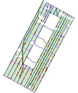
Figure 2: Street network in the considered area. Charging stations are red, one way roads green, and two-way roads blue.

We consider the area in the middle of Manhattan, from 42nd to 116th Street, see Fig. 2. Street intersections and directions of feasible movement form the state and action spaces of the MDP. Intersections in the proximity of real-world fast charging stations [56] represent the set of reload states.

Figure 3: Transition from intersection $I_{1}$ to $I_{2}$ with stochastic consumption. The small circles are dummy states.

After the AEV picks a direction, it reaches the next intersection in that direction deterministically with a stochastic energy consumption. We base our model of consumption on distributions of vehicle travel times from the area [55] and conversion of velocity and travel times to energy consumption [52]. We discretize the consumption distribution into three possible values ($c_{1},c_{2},c_{3}$) reached with corresponding probabilities ($p_{1},p_{2},p_{3}$). The transition from one intersection ($I_{1}$) to another ($I_{2}$) is then modelled using three dummy states as explained in Fig. 3.

In this fashion, we model the street network of Manhattan as a CMDP with with $7378$ states and $8473$ actions. For a fixed set of 100 randomly selected target states, Fig. 4 shows influence of requested capacity on running times for (a) strategy for Büchi objective using CMDP (our approach), and (b) MEC-decomposition for the corresponding explicit MDP. We can see from the plots that our algorithm runs reasonably fast for all capacities (it stabilizes for $\mathit{cap}>95$), it is not the case for the explicit approach. The running times for MEC-decomposition is dependent on the numbers of states and actions in the explicit MDP, which keep growing. The number of states of the explicit MDP for capacity 95 is 527475, while it is still only 7378 in the original CMDP. Also note that actually solving the Büchi objective in the explicit MDP requires computing almost-sure reachability of MECs with some target states. Therefore, we can expect that even for small capacities our approach would outperform the explicit one (Fig. 4 (c)).

Figure 4: Mean computation times for a fixed target set of size 100 and varying capacity: (a) CMDP – computating Büchi objective via CMDP, (b) explicit – computating MEC decomposition of the explicit MDP, (c) combined – (a) and (b) combined for small capacity values.

7.2 Multi-agent Grid World

We use multi-agent grid world to generate CMDP with huge number of states to reach the scalability limits of the proposed algorithms. We model the rover and the helicopter of the Mars 2020 mission with the following realistic considerations: the rover enjoys infinite energy while the helicopter is restricted by batteries recharged at the rover. These two vehicle jointly operate on a mission where the helicopter reaches areas inaccessible to the rover. The outcomes of the helicopter’s actions are deterministic while those of the rover — influenced by terrain dynamics — are stochastic. For a grid world of size $n$, this system can be naturally modeled as a CMDP with $n^{4}$ states. Fig. 5 shows the running times of the Büchi objective for growing grid sizes and capacities in CMDP. It also shows the running time for the MEC decomposition of the corresponding explicit MDP when the capacity is 10. We observe that the increase in the computational time of CMDP follows the growth in the number of states roughly linearly, and our implementation deals with an MDP with $1.6\times 10^{5}$ states in no more than seven minutes.

Figure 5: Mean computation times for varying grid sizes and of size capacities: (a) CMDP – computating Büchi objective via CMDP, (b) explicit – computating MEC decomposition of the explicit MDP for a capacity of 10, (c) combined – combined computation time for a capacity of 10.

8 Conclusion & Future Work

We presented a first study of consumption Markov decision processes (CMDPs) with qualitative $\omega$-regular objectives. We developed and implemented a polynomial-time algorithm for CMDPs with an objective of probability-1 satisfaction of a given Büchi condition. Possible directions for the future work are extensions to quantitative analysis (e.g. minimizing the expected resource consumption), stochastic games, or partially observable setting.

Acknowledgements: We acknowledge the kind help of Vojtěch Forejt, David Klaška, and Martin Kučera in the discussions leading to this paper.

Technical Appendix

Appendix 0.A Proofs

0.A.1 Proof of Theorem 4.1

Lemma 8

There exists a memory-less optimal strategy for the objective $\mathit{MinReach}_{T}$.

Proof

It is clear that in every state $s$, the player must play a good action, i.e. an action $a$ such that $C(s,a)+\max_{s^{\prime}\in\mathit{Succ}(s,a)}\mathit{MinReach}_{T}(s^{\prime})\leq\mathit{MinReach}_{T}(s)$. If there are multiple good actions in some state $s$ we proceed as follows.

We first assign a ranking to states. All states in $T$ have rank $0$. Now assume that we have assigned ranks $\leq i$ and we want to assign rank $i+1$ to some of the yet unranked states. We say that an action $a$ is progressing in an unranked state $s$ if all $s^{\prime}\in\mathit{Succ}(s,a)$ have a rank (smaller than $i+1$). If all good actions in the yet unranked states are non-progressing, than all the unranked states $s$ have $\mathit{MinReach}_{T}(s)=\infty$, since by playing any good action, the player cannot force reaching a ranked state and thus also a target state; hence, in this case we assign all the unranked states the rank $\infty$ and finish the construction. Otherwise, we assign rank $i+1$ to all unranked states that have a good progressing action and continue with the construction. It is easy to see that a state $s$ is assigned a finite rank if and only if $\mathit{MinReach}_{T}(s)<\infty$.

We now fix a memory-less strategy $\sigma$ such that in a state of finite rank, $\sigma$ chooses a good progressing action; for states of an infinite rank, $\sigma$ chooses an arbitrary (but fixed) action. Since $\sigma$ only uses good actions, a straightforward induction shows that for each state $s$ and each $s$-initiated run that reaches $T$ actually reaches $T$ with consumption at most $\mathit{MinReach}_{T}(s)$. So we need to show that $\sigma$ does not admit runs initiated in a state of finite rank that never reach $T$. But all $\sigma$-compatible runs initiated in a state of finite rank decrease the rank in every step, since $\sigma$ only plays progressing actions. The result follows. ∎

Given a target set $T$, a number $i\in\mathbb{N}$, and a run $\mathit{\varrho}$, we define $\mathit{ReachCons}_{T}^{i}(\mathit{\varrho})$ as $\mathit{ReachCons}_{T}(\mathit{\varrho})$ with the additional restriction that $f\leq i$. Intuitively, $\mathit{ReachCons}_{T}^{i}(\mathit{\varrho})=\infty$ if $\mathit{\varrho}$ does not visit $T$ withing $i-1$ steps. We then put

$$\mathit{MinReach}_{T}^{i}(s)=\inf_{\sigma}\sup_{\mathit{\varrho}\in\mathsf{Comp}(\sigma,s)}\mathit{ReachCons}_{T}^{i}(\mathit{\varrho}).$$

Lemma 9

For every $i\geq 0$ it holds that $\mathit{MinReach}_{T}^{i}(s)=\mathcal{F}^{i}(\mathbf{x}_{T})(s)$.

Proof

By an induction on $i$. The base case is simple. Now assume that the equality holds for some $i\geq 0$. For $i+1$ we get:

∎

Theorem 4.1. Denote by $n$ the length of the longest simple path in $\mathcal{M}$. Let $\mathbf{x}_{T}$ be a vector such that $\mathbf{x}_{T}(s)=0$ if $s\in T$ and $\mathbf{x}_{T}(s)=\infty$ otherwise. Then iterating $\mathcal{F}$ on $\mathbf{x}_{T}$ yields a fixpoint in at most $n$ steps and this fixpoint equals $\mathit{MinReach}_{T}$.

Proof

It is easy to see that for each $s$ and each $i\geq 0$ it holds that $\mathit{MinReach}_{T}^{i}(s)\geq\mathit{MinReach}_{T}(s)$. Furthermore, an easy computation shows that $\mathit{MinReach}_{T}(s)$ is a fixed point of $\mathcal{F}$. Hence, it suffices to show that $\mathit{MinReach}_{T}^{|S|}(s)=\mathit{MinReach}_{T}(s)$. Assume, for the sake of contradiction, that we have some $s\in S$ such that $\mathit{MinReach}_{T}^{|S|}(s)>\mathit{MinReach}_{T}(s)$. Fix $\sigma$ to be the memory-less optimal strategy from Lemma 8. By the definition of $\mathit{MinReach}_{T}^{|S|}(s)$ we have a run $\mathit{\varrho}\in\mathsf{Comp}(\sigma,s)$ such that $\mathit{ReachCons}_{T}^{|S|}(\mathit{\varrho})>\mathit{MinReach}_{T}(s)$. This is only possible if $\mathit{ReachCons}_{T}^{|S|}(\mathit{\varrho})=\infty$, otherwise this would contradict the optimality of $\sigma$ (note that if $\mathit{ReachCons}_{T}^{i}(\mathit{\varrho})<\infty$, then $\mathit{ReachCons}_{T}^{j}(\mathit{\varrho})=\mathit{ReachCons}_{T}^{i}(\mathit{\varrho})$ for all $j\geq i$). Hence, there is a run compatible with $\sigma$ whose prefix of length $|S|$ does not contain a target state. But this prefix must contain a cycle, and since $\sigma$ is memory-less, we can iterate this cycle forever. Hence, the optimal strategy $\sigma$ admits a run from $s$ that never reaches $T$, a contradiction with $\mathit{MinReach}_{T}(s)<\mathit{MinReach}_{T}^{|S|}(s)\leq\infty$.∎

0.A.2 Proof of Lemma 3

By induction on $i$. The base case is clear. Now assume that the equality holds for some $i\geq 0$. Note that for any $(s,a)\in S\times A$ we have $\mathit{Succ}(\tilde{s},a)=\mathit{Succ}(s,a)\subseteq S$. Also, for all $s^{\prime}\in S\setminus\mathit{R}$ we have $\llfloor\,\mathcal{G}^{i}(\boldsymbol{\infty})\,\rrfloor{}(s^{\prime})={\mathcal{G}^{i}(\boldsymbol{\infty})}(s^{\prime})=\mathcal{F}^{i}(\mathbf{x}_{\mathit{R}})(s^{\prime})$ (by induction hypothesis), while for $s^{\prime}\in S\cap\mathit{R}$ we have $\llfloor\,\mathcal{G}^{i}(\boldsymbol{\infty})\,\rrfloor{}(s^{\prime})=0=\mathcal{F}^{i}(\mathbf{x}_{\mathit{R}})(s^{\prime})$ (by the definition of $\mathcal{F}$). Hence, $\max_{s^{\prime}\in\mathit{Succ}(s,a)}\llfloor\,\mathcal{G}^{i}(\boldsymbol{\infty})\,\rrfloor{}(s^{\prime})=\max_{s^{\prime}\in\mathit{Succ}(\tilde{s},a)}{\mathcal{F}^{i}(\mathbf{x}_{\mathit{R}})(s^{\prime})}$. Thus,

$$\mathcal{G}^{i+1}(\boldsymbol{\infty})(s) =\min_{a\in A}\left(C(s,a)+\max_{s^{\prime}\in\mathit{Succ}(s,a)}\llfloor\,\mathcal{G}^{i}(\boldsymbol{\infty})\,\rrfloor{}(s^{\prime})$$

$$=\min_{a\in A}\left(C(s,a)+\max_{s^{\prime}\in\mathit{Succ}(\tilde{s},a)}{\mathcal{F}^{i}(\mathbf{x}_{\mathit{R}})(s^{\prime})}\right)$$

$$=\mathcal{F}^{i+1}(\mathbf{x}_{\mathit{R}})(\tilde{s}).$$

(The last equation following from the definition of $\mathcal{F}$ and from the fact that $\tilde{s}$ is never a reload state.)

Moreover, from Lemma 9 it follows that $\mathcal{F}^{i+1}(\mathbf{x}_{\mathit{R}})(s)=\mathit{MinReach}_{\mathit{R}}^{i+1}(s)$. But if $s$ is not a reload state, then $\mathit{MinReach}_{\mathit{R}}^{i+1}(s)=\mathit{MinReach}_{\mathit{R}}^{i+1}(\tilde{s})$, so for $s\in S\setminus\mathit{R}$ we have $\mathcal{G}^{i+1}(\boldsymbol{\infty})(s)=\mathcal{F}^{i+1}(\mathbf{x}_{\mathit{R}})(\tilde{s})=\mathcal{F}^{i+1}(\mathbf{x}_{\mathit{R}})(s)$, which proves the second part. ∎

0.A.3 Completion of the proof of Theorem 4.3

Now we prove that upon termination, $\mathbf{out}\geq\mathit{Safe}_{\mathcal{M}}$. For every $t\in S$ there exists, by the definition of $\mathit{MinInitCons}$, a strategy $\sigma_{t}$ s.t. $\mathit{ReachCons}_{\mathcal{M}(\mathit{Rel}),\mathit{Rel}}^{+}(\sigma_{t},t)=\mathbf{mic}(t)=\mathbf{out}(t)$ and thus $\mathit{ReachCons}_{\mathcal{M}(\mathit{Rel}),\mathit{Rel}}^{+}(\mathit{\varrho})$ is bounded by $\mathbf{out}(t)$ for each $\mathit{\varrho}\in\mathsf{Comp}(\sigma_{t},t)$. We construct a new strategy $\pi$ that, starting in some state $t$ initially mimics $\sigma_{t}$ until the next visit of a state $r_{1}\in\mathit{Rel}$. Once this happens, the strategy $\pi$ begins to mimic $\sigma_{r_{1}}$ until the next visit of some $r_{2}\in\mathit{Rel}$, when $\pi$ begins to mimic $\sigma_{r_{2}}$, and so on ad infinitum.

Fix any state $s$ such that upon termination, $\mathbf{mic}(s)\leq\mathit{cap}$ (for other states, the inequality $\mathbf{out}(s)\geq\mathit{Safe}_{\mathcal{M}}(s)$ clearly holds). We prove that every run $\mathit{\varrho}\in\mathsf{Comp}_{\mathcal{M}(\mathit{Rel})}(\pi,s)$ is actually $\mathbf{mic}(s)$-safe from $s$ in the original MDP $\mathcal{M}$. In fact, it is sufficient to show this in $\mathcal{M}(\mathit{Rel})$, since each its reload state is also a reload state of $\mathcal{M}$.

Let $i_{1}<i_{2}<\ldots$ be all indices $i$ such that $\mathit{\varrho}_{i}\in\mathit{Rel}$. Since $\pi$ mimics $\sigma_{s}$ until $\mathit{\varrho}_{i_{1}}$, we have that $\mathit{RL}_{\mathbf{mic}(s)}(\mathit{\varrho}_{..j})=\mathbf{mic}(s)-\mathit{cons}(\mathit{\varrho}_{..j})$ where $\mathit{cons}(\mathit{\varrho}_{..j})$ is by definition of $\sigma_{s}$ bounded by $\mathbf{mic}(s)$, for all $j\leq i_{1}$. Now let $m\geq 1$, we set $k=i_{m}$ and $l=i_{m+1}$. As $\pi$ mimics $\sigma_{\mathit{\varrho}_{k}}$ for between $\mathit{\varrho}_{k}$ and $\mathit{\varrho}_{l}$ we have for $k<j\leq l$ that $\mathit{RL}_{\mathbf{mic}(s)}(\mathit{\varrho}_{..j})=\mathit{RL}_{\mathit{cap}}(\mathit{\varrho}_{k..j})=\mathit{cap}-\mathit{cons}(\mathit{\varrho}_{k..j})$, where $\mathit{cons}(\mathit{\varrho}_{k..j})$ is bounded by $\mathit{ReachCons}_{\mathit{Rel}}^{+}(\sigma_{\mathit{\varrho}_{k}},\mathit{\varrho}_{k})=\mathbf{mic}(\mathit{\varrho}_{k})<\mathit{cap}$. Therefore, $\mathit{RL}_{\mathbf{mic}(s)}(\mathit{\varrho}_{..j})\geq 0$ for all $j$ and $\mathit{\varrho}$ is $\mathbf{mic}(s)$-safe. This finishes the proof. ∎

0.A.4 Proof of Lemma 4

By induction on $i$. The base case is clear. Now assume that the statement holds for some $i\geq 0$. Fix any $s$. Denote by $b=\mathcal{B}^{i+1}(\mathbf{y}_{T})(s)$ and $d=\mathit{SafePR}_{T}^{i+1}(s)$. We show that $b=d$. The equality holds whenever $s\in T$, so in the remainder of the proof we assume that $s\not\in T$.

We first prove that $b\geq d$. If $b=\infty$, this is clearly true. Otherwise, let $a_{\min}$ be the action minimizing $\mathit{SPR\textnormal{-}Val}(s,a_{\min},\mathcal{B}^{i}(\mathbf{y}_{T}))$ (which equals $b$ if $s\not\in\mathit{R}$) and let $t_{\min}\in\mathit{Succ}(s,a_{\min})$ be the successor used to achieve this value. By induction hypothesis, there exists a strategy $\sigma_{1}$ that is $\mathcal{B}^{i}(\mathbf{y}_{T})(t_{\min})$-safe in $t_{\min}$ and $\mathbb{P}^{\sigma_{1}}_{t_{\min}}(\mathsf{Reach}_{T}^{i})>0$, and there also exists a strategy $\sigma_{2}$ that is $\mathit{Safe}(t)$-safe from $t$ for all $t\in\mathit{Succ}(s,a_{\min}),t\neq t_{\min}$.

Consider now a strategy $\pi$ which, starting in $s$, plays $a_{\min}$. If the outcome of $a_{\min}$ is $t_{\min}$, $\pi$ starts to mimic $\sigma_{1}$, otherwise it starts to mimic $\sigma_{2}$. We claim that $\pi$ is $b$-safe in $s$ and that $\mathbb{P}^{\pi}_{s}(\mathsf{Reach}_{T}^{i+1})>0$ by showing the following two points.

1. There is at least one run $\mathit{\varrho}_{T}\in\mathsf{Comp}(\pi,s)$ that reaches $T$ in $\leq i+1$ steps.

2. All runs in $\mathsf{Comp}(\pi,s)$ are $b$-safe.

We construct $\mathit{\varrho}_{T}$ easily as $\mathit{\varrho}_{T}=\alpha\odot\mathit{\varrho}^{\prime}$ where $\alpha=sa_{\min}t_{\min}$ and $\mathit{\varrho}^{\prime}$ is the witness that $\mathbb{P}^{\sigma_{1}}_{t_{\min}}(\mathsf{Reach}_{T}^{i})>0$. Now let $\mathit{\varrho}\in\mathsf{Comp}(\pi,s)$ be a run produced by $\pi$ from $s$. Then it has to be of the form $\mathit{\varrho}=sa_{\min}t\odot\mathit{\varrho}_{\sigma}$ where $\mathit{\varrho}_{\sigma}\in\mathsf{Comp}(\sigma_{1},t)$ if $t=t_{\min}$ or $\mathit{\varrho}_{\sigma}\in\mathsf{Comp}(\sigma_{2},t)$ it $t\neq t_{\min}$; in both cases $\mathit{Safe}(t)$-safe in $t$. By definition of $\mathit{SPR\textnormal{-}Val}$ and by induction hypothesis, we have for $s\notin\mathit{R}$ that $b\geq C(s,a_{\min})+\mathit{Safe}(t)$ and thus $\mathit{RL}_{b}(sa_{\min}t)\geq\mathit{Safe}(t)$ and thus $\mathit{\varrho}$ is $b$-safe by Lemma 1. If $s\in\mathit{R}$ and $b=0$, by similar arguments, as $C(s,a_{\min})+\mathit{Safe}(t)\leq\mathit{cap}$ (otherwise $b$ would be $\infty$), we have that $\mathit{RL}_{b}(sa_{\min}t)\geq\mathit{Safe}(t)$ and thus $\mathit{\varrho}$ is $b$-safe.

Now we prove that $b\leq d$. This clearly holds if $d=\infty$, so in the remainder of the proof we assume $d\leq\mathit{cap}(\mathcal{M})$. By the definition of $d$ there exists a strategy $\sigma$ s.t. $\sigma$ is $d$-safe in $s$ and $\mathbb{P}^{\sigma}_{s}(\mathsf{Reach}_{T}^{i+1}(d))>0.$ Let $a=\sigma(a)$ be the action selected by $\sigma$ in the first step when starting in $s$. We denote by $\tau$ the strategy such that for all histories $\alpha$ we have $\tau(\alpha)=\sigma(sa\alpha)$. For each $t\in\mathit{Succ}(s,a)$ we assign a number $d_{t}$ defined as $d_{t}=0$ if $t\in\mathit{R}$ and $d_{t}=\mathit{RL}_{d}(sat)$ otherwise.

We finish the proof by proving these two claims:

1. It holds $\mathit{SPR\textnormal{-}Val}(s,a,\mathcal{B}^{i}(\mathbf{y}_{T}))\leq C(s,a)+\max_{t\in\mathit{Succ}(s,a)}d_{t}$.

2. If $s\not\in\mathit{R}$, then $C(s,a)+\max_{t\in\mathit{Succ}(s,a)}d_{t}\leq d$.

Let us first see, why these claims are indeed sufficient. From (1.) we get $\mathcal{A}(\mathcal{B}^{i}(\mathbf{y}_{T}))(s)\leq C(s,a)+\max_{t\in\mathit{Succ}(s,a)}d_{t}\leq\mathit{cap}(\mathcal{M})$ (from the definition of $\mathit{RL}_{d}(sat)$). If $s\in\mathit{R}$, then it follows that $\llbracket\,\mathcal{A}(\mathcal{B}^{i}(\mathbf{y}_{T}))\,\rrbracket(s)=0\leq d$. If $s\not\in\mathit{R}$, then $\llbracket\,\mathcal{A}(\mathcal{B}^{i}(\mathbf{y}_{T}))\,\rrbracket(s)=\mathcal{A}(\mathcal{B}^{i}(\mathbf{y}_{T}))(s)\leq C(s,a)+\max_{t\in\mathit{Succ}(s,a)}d_{t}\leq d$, the first inequality shown above and the second coming from (2.).

So let us start with proving (1.). Note that for each $t\in\mathit{Succ}(s,a)$, $\tau$ is necessarily $d_{t}$-safe from $t$; hence, $\mathit{Safe}(t)\leq d_{t}$. Moreover, there exists $q\in\mathit{Succ}(s,a)$ s.t. $\mathbb{P}^{\tau}_{q}(\mathsf{Reach}_{T}^{i})>0$; hence, by induction hypothesis it holds $\mathcal{B}^{i}(\mathbf{y}_{T})(q)\leq d_{q}$. From this and from the definition of $\mathit{SPR\textnormal{-}Val}$ we get

$$\mathit{SPR\textnormal{-}Val}(s,a,\mathcal{B}^{i}(\mathbf{y}_{T}) \leq C(s,a)+\max\{\mathcal{B}^{i}(\mathbf{y}_{T})(q),\mathit{Safe}(t)\mid t\in\mathit{Succ}(s,a),t\neq q\}$$

$$\leq C(s,a)+\max_{t\in\mathit{Succ}(s,a)}d_{t}.$$

To finish, (2.) follows immediately from the definition of $d_{t}$ and $\mathit{RL}_{d}(sat)$ as $\mathit{RL}_{d}(sat)$ is always bounded from above by $d-\mathit{cap}(s,a)$ for $s\notin\mathit{R}$. ∎

0.A.5 Proof of Lemma 5

By Lemma 4, it suffices to show that $\mathit{SafePR}_{T}=\mathit{SafePR}_{T}^{K}$. To this end, fix any state $s$ such that $\mathit{SafePR}_{T}(s)<\infty$. For the sake of succinctness, we denote $\mathit{SafePR}_{T}(s)=d$. To any strategy $\pi$ that is $d$-safe in $s$, we assign its index, which is the infimum of all $i$ such that $\mathbb{P}^{\pi}_{s}(\mathsf{Reach}_{T}^{i})>0$. By assumption that $\mathit{SafePR}_{T}(s)<\infty$, there is at least one $\pi$ with a finite index. Let $\sigma$ be the $d$-safe in $s$ strategy with minimal index $i$: we show that the $i\leq K$.

We proceed by a suitable “strategy surgery” on $\sigma$. Let $\alpha$ be a history produced by $\sigma$ from $s$ of length $i$ whose last state belongs to $T$. Assume, for the sake of contradiction, that $i>K$. This can only be if at least one of the following conditions hold:

1. Some reload state is visited twice on $\alpha$, i.e. there are $0\leq j<k\leq i+1$ such that $\alpha_{k}=\alpha_{j}\in\mathit{R}$, or

2. some state is visited twice with no intermediate visits to a reload state; i.e., there are $0\leq j<k\leq i+1$ such that $\alpha_{k}=\alpha_{j}$ and $\alpha_{\ell}\not\in\mathit{R}$ for all $j<\ell<k$.

Indeed, if none of the conditions hold, then the reload states partition $\alpha$ into at most $|\mathit{R}|+1$ segments, each segment containing non-reload states without repetition. This would imply $i=len(\alpha)\leq K$.

In both cases (a) and (b) we can arrive at a contradiction using essentially the same argument. Let us illustrate the details on case (a): Consider a strategy $\pi$ such that for every history of the form $\alpha_{..j}\odot\gamma$ for a suitable $\gamma$ we have $\pi(\alpha_{..j}\odot\gamma)=\sigma(\alpha_{..k}\odot\gamma)$; on all other histories, $\pi$ mimics $\sigma$. Then $\pi$ is still $d$-safe in $s$. Indeed, the behavior only changed on the suffixes of $\alpha_{..j}$, and for each suitable $\gamma$ we have $\mathit{RL}_{d}(\alpha_{..j}\odot\gamma)=\mathit{RL}_{d}(\alpha_{..j}\odot\gamma)$ due to the fact that $\alpha_{j}=\alpha_{k}$ is a reload state. But $\pi$ has index $i-(k-j)<i$, a contradiction with the choice of $\sigma$.

For case (b), the only difference is that now the resource level after $\alpha_{..j}\odot\gamma$ can be higher then the one of $\alpha_{..k}\odot\gamma$ due to the removal of the intermediate non-reloading cycle. Since we need to show that the energy level never drops below 0, the same argument works.∎

References

- [1] P. A. Abdulla, M. F. Atig, P. Hofman, R. Mayr, K. N. Kumar, and P. Totzke. Infinite-state energy games. In Joint Meeting of the 23rd EACSL Annual Conference on Computer Science Logic and the 29th Annual ACM/IEEE Symposium on Logic in Computer Science, pages 7:1–7:10, 2014.
- [2] R. Ash and C. Doléans-Dade. Probability and Measure Theory. Harcourt/Academic Press, 2000.
- [3] G. Bacci, P. Bouyer, U. Fahrenberg, K. G. Larsen, N. Markey, and P.-A. Reynier. Optimal and robust controller synthesis. In K. Havelund, J. Peleska, B. Roscoe, and E. de Vink, editors, Formal Methods, pages 203–221. Springer, 2018.
- [4] C. Baier, P. Chrszon, C. Dubslaff, J. Klein, and S. Klüppelholz. Energy-utility analysis of probabilistic systems with exogenous coordination. In F. de Boer, M. Bonsangue, and J. Rutten, editors, It’s All About Coordination, pages 38–56. Springer International Publishing, 2018.
- [5] C. Baier, M. Daum, C. Dubslaff, J. Klein, and S. Klüppelholz. Energy-utility quantiles. In 6th International Symposium on NASA Formal Methods, pages 285–299, 2014.
- [6] C. Baier, C. Dubslaff, J. Klein, S. Klüppelholz, and S. Wunderlich. Probabilistic model checking for energy-utility analysis. In F. van Breugel, E. Kashefi, C. Palamidessi, and J. Rutten, editors, Horizons of the Mind: A Tribute to Prakash Panangaden, pages 96–123. Springer, 2014.
- [7] C. Baier, C. Dubslaff, S. Klüppelholz, and L. Leuschner. Energy-utility analysis for resilient systems using probabilistic model checking. In 35th International Conference on Application and Theory of Petri Nets and Concurrency, pages 20–39, 2014.
- [8] B. Balaram, T. Canham, C. Duncan, H. F. Grip, W. Johnson, J. Maki, A. Quon, R. Stern, and D. Zhu. Mars helicopter technology demonstrator. In AIAA Atmospheric Flight Mechanics Conference, 2018.
- [9] U. Boker, T. A. Henzinger, and A. Radhakrishna. Battery transition systems. In 41st ACM SIGPLAN-SIGACT Symposium on Principles of Programming Languages, pages 595–606, 2014.
- [10] P. Bouyer, U. Fahrenberg, K. G. Larsen, and N. Markey. Timed automata with observers under energy constraints. In 13th ACM International Conference on Hybrid Systems: Computation and Control, pages 61–70. ACM, 2010.
- [11] P. Bouyer, U. Fahrenberg, K. G. Larsen, N. Markey, and J. Srba. Infinite Runs in Weighted Timed Automata with Energy Constraints. In 6th International Conference on Formal Modelling and Analysis of Timed Systems Co-located, pages 33–47, 2008.
- [12] P. Bouyer, P. Hofman, N. Markey, M. Randour, and M. Zimmermann. Bounding average-energy games. In J. Esparza and A. S. Murawski, editors, 20th International Conference on Foundations of Software Science and Computation Structures, pages 179–195, 2017.
- [13] P. Bouyer, N. Markey, M. Randour, K. G. Larsen, and S. Laursen. Average-energy games. Acta Informatica, 55(2):91–127, Mar 2018.
- [14] T. Brázdil, K. Chatterjee, A. Kučera, and P. Novotný. Efficient controller synthesis for consumption games with multiple resource types. In Computer Aided Verification, pages 23–38, 2012.
- [15] T. Brázdil, P. Jančar, and A. Kučera. Reachability games on extended vector addition systems with states. In 37th International Colloquium on Automata, Languages, and Programming, pages 478–489, 2010.
- [16] T. Brázdil, D. Klaška, A. Kučera, and P. Novotný. Minimizing running costs in consumption systems. In Computer Aided Verification, pages 457–472, 2014.
- [17] T. Brázdil, A. Kučera, and P. Novotný. Optimizing the expected mean payoff in energy Markov decision processes. In 14th International Symposium on Automated Technology for Verification and Analysis, pages 32–49.
- [18] R. Brenguier, F. Cassez, and J.-F. Raskin. Energy and mean-payoff timed games. In 17th International Conference on Hybrid Systems: Computation and Control, page 283–292, 2014.
- [19] T. Brihaye, G. Geeraerts, A. Haddad, and B. Monmege. Pseudopolynomial iterative algorithm to solve total-payoff games and min-cost reachability games. Acta Informatica, 54(1):85–125, 2017.
- [20] L. Brim, J. Chaloupka, L. Doyen, R. Gentilini, and J. Raskin. Faster algorithms for mean-payoff games. Formal Methods in System Design, 38(2):97–118, 2011.
- [21] V. Bruyère, Q. Hautem, M. Randour, and J.-F. Raskin. Energy mean-payoff games. In 30th International Conference on Concurrency Theory, pages 21:1–21:17, 2019.
- [22] D. Cachera, U. Fahrenberg, and A. Legay. An -algebra for real-time energy problems. Logical Methods in Computer Science, 15(2), 2019.
- [23] A. Chakrabarti, L. de Alfaro, T. A. Henzinger, and M. Stoelinga. Resource interfaces. In 3rd International Workshop on Embedded Software, pages 117–133, 2003.
- [24] J. Chaloupka. Z-reachability problem for games on 2-dimensional vector addition systems with states is in P. Fundamenta Informaticae, 123(1):15–42, 2013.
- [25] K. Chatterjee. Stochastic -regular games. PhD thesis, University of California, Berkeley, 2007.
- [26] K. Chatterjee and L. Doyen. Energy and Mean-Payoff Parity Markov Decision Processes. In 36th International Symposium on Mathematical Foundations of Computer Science, pages 206–218, 2011.
- [27] K. Chatterjee and L. Doyen. Energy parity games. Theoretical Computer Science, 458:49–60, 2012.
- [28] K. Chatterjee, L. Doyen, T. Henzinger, and J.-F. Raskin. Generalized mean-payoff and energy games. In 30th Annual Conference on Foundations of Software Technology and Theoretical Computer Science, pages 505–516, 2010.
- [29] K. Chatterjee, M. Henzinger, S. Krinninger, and D. Nanongkai. Polynomial-Time Algorithms for Energy Games with Special Weight Structures. In 20th Annual European Symposium on Algorithms, pages 301–312, 2012.
- [30] K. Chatterjee, M. Jurdziński, and T. Henzinger. Quantitative stochastic parity games. In 15th Annual ACM-SIAM Symposium on Discrete Algorithms, pages 121–130, 2004.
- [31] K. Chatterjee, M. Randour, and J.-F. Raskin. Strategy synthesis for multi-dimensional quantitative objectives. Acta informatica, 51(3-4):129–163, 2014.
- [32] C. Courcoubetis and M. Yannakakis. The complexity of probabilistic verification. Journal of the ACM, 42(4):857–907, 1995.
- [33] L. de Alfaro. Formal verification of probabilistic systems. PhD thesis, Stanford University, 1998.
- [34] A. Degorre, L. Doyen, R. Gentilini, J.-F. Raskin, and S. Toruńczyk. Energy and mean-payoff games with imperfect information. In 24th International Workshop on Computer Science Logic, pages 260–274, 2010.
- [35] Z. Ésik, U. Fahrenberg, A. Legay, and K. Quaas. An algebraic approach to energy problems I – continuous Kleene -algebras. Acta Cybernetica, 23(1):203–228, 2017.
- [36] Z. Ésik, U. Fahrenberg, A. Legay, and K. Quaas. An algebraic approach to energy problems II – the algebra of energy functions. Acta Cybernetica, 23(1):229–268, 2017.
- [37] U. Fahrenberg, L. Juhl, K. G. Larsen, and J. Srba. Energy games in multiweighted automata. In 8th International Colloquium on Theoretical Aspects of Computing, pages 95–115, 2011.
- [38] U. Fahrenberg and A. Legay. Featured weighted automata. In 5th International FME Workshop on Formal Methods in Software Engineering, pages 51–57, 2017.
- [39] N. Fijalkow and M. Zimmermann. Cost-parity and cost-Streett games. In 32nd Annual Conference on Foundations of Software Technology and Theoretical Computer Science, pages 124–135, 2012.
- [40] E. Filiot, R. Gentilini, and J.-F. Raskin. Quantitative languages defined by functional automata. In M. Koutny and I. Ulidowski, editors, 23rd International Conference on Concurrency Theory, pages 132–146, 2012.
- [41] E. M. Hahn, M. Perez, F. Somenzi, A. Trivedi, S. Schewe, and D. Wojtczak. Good-for-MDPs automata for probabilistic analysis and reinforcement learning. In 26th International Conference on Tools and Algorithms for the Construction and Analysis of Systems, 2020.
- [42] L. Herrmann, C. Baier, C. Fetzer, S. Klüppelholz, and M. Napierkowski. Formal parameter synthesis for energy-utility-optimal fault tolerance. In 15th European Performance Engineering Workshop, pages 78–93, 2018.
- [43] L. Juhl, K. G. Larsen, and J.-F. Raskin. Optimal bounds for multiweighted and parametrised energy games. In Z. Liu, J. Woodcock, and H. Zhu, editors, Theories of Programming and Formal Methods, pages 244–255. Springer, 2013.
- [44] M. Jurdziński, R. Lazić, and S. Schmitz. Fixed-dimensional energy games are in pseudo-polynomial time. In 42nd International Colloquium on Automata, Languages, and Programming, pages 260–272, 2015.
- [45] M. Jurdziński. Deciding the winner in parity games is in UP co-UP. Information Processing Letters, 68(3):119 – 124, 1998.
- [46] L. Khachiyan, E. Boros, K. Borys, K. Elbassioni, V. Gurvich, G. Rudolf, and J. Zhao. On short paths interdiction problems: Total and node-wise limited interdiction. Theory of Computing Systems, 43(2):204–233, 2008.
- [47] D. Klaška. Complexity of Consumption Games. Bachelor’s thesis, Masaryk University, 2014.
- [48] K. G. Larsen, S. Laursen, and M. Zimmermann. Limit your consumption! Finding bounds in average-energy games. In 14th International Workshop Quantitative Aspects of Programming Languages and Systems, pages 1–14, 2016.
- [49] R. Mayr, S. Schewe, P. Totzke, and D. Wojtczak. MDPs with energy-parity objectives. In 32nd Annual ACM/IEEE Symposium on Logic in Computer Science, pages 1–12, 2017.
- [50] Project Jupyter, M. Bussonnier, J. Forde, J. Freeman, B. Granger, T. Head, C. Holdgraf, K. Kelley, G. Nalvarte, A. Osheroff, M. Pacer, Y. Panda, F. Perez, B. Ragan-Kelley, and C. Willing. Binder 2.0 – reproducible, interactive, sharable environments for science at scale. In 17th Python in Science Conference, pages 113 – 120, 2018.
- [51] S. Sickert, J. Esparza, S. Jaax, and J. Křetínský. Limit-deterministic Büchi automata for linear temporal logic. In Computer Aided Verification, pages 312–332, 2016.
- [52] J. B. Straubel. Roadster efficiency and range. https://www.tesla.com/blog/roadster-efficiency-and-range, 2008.
- [53] G. Sugumar, R. Selvamuthukumaran, T. Dragicevic, U. Nyman, K. G. Larsen, and F. Blaabjerg. Formal validation of supervisory energy management systems for microgrids. In 43rd Annual Conference of the IEEE Industrial Electronics Society, pages 1154–1159, 2017.
- [54] R. S. Sutton and A. G. Barto. Reinforcement Learning: An Introduction. MIT Press, 2018.
- [55] Uber Movement. Traffic speed data for New York City. https://movement.uber.com/, 2019.
- [56] United States Department of Energy. Alternative fuels data center. https://afdc.energy.gov/stations/, 2019.
- [57] Y. Velner, K. Chatterjee, L. Doyen, T. A. Henzinger, A. M. Rabinovich, and J. Raskin. The complexity of multi-mean-payoff and multi-energy games. Information and Computation, 241:177–196, 2015.
- [58] E. R. Wognsen, R. R. Hansen, K. G. Larsen, and P. Koch. Energy-aware scheduling of FIR filter structures using a timed automata model. In 19th International Symposium on Design and Diagnostics of Electronic Circuits and Systems, pages 1–6, 2016.
- [59] H. Zhang, C. J. R. Sheppard, T. E. Lipman, and S. J. Moura. Joint fleet sizing and charging system planning for autonomous electric vehicles. IEEE Transactions on Intelligent Transportation Systems, 2019.