A Gas Giant Planet in the OGLE-2006-BLG-284L Stellar Binary System

Abstract

We present the analysis of microlensing event OGLE-2006-BLG-284, which has a lens system that consists of two stars and a gas giant planet with a mass ratio of $q_{p}=(1.26\pm 0.19)\times 10^{-3}$ to the primary. The mass ratio of the two stars is $q_{s}=0.289\pm 0.011$, and their projected separation is $s_{s}=2.1\pm 0.7\,$AU, while the projected separation of the planet from the primary is $s_{p}=2.2\pm 0.8\,$AU. For this lens system to have stable orbits, the three-dimensional separation of either the primary and secondary stars or the planet and primary star must be much larger than that these projected separations. Since we do not know which is the case, the system could include either a circumbinary or a circumstellar planet. Because there is no measurement of the microlensing parallax effect or lens system brightness, we can only make a rough Bayesian estimate of the lens system masses and brightness. We find host star and planet masses of $M_{L1}=0.35^{+0.30}_{-0.20}\,M_{\odot}$, $M_{L2}=0.10^{+0.09}_{-0.06}\,M_{\odot}$, and $m_{p}=144^{+126}_{-82}\,{M_{\oplus}}$, and the $K$-band magnitude of the combined brightness of the host stars is $K_{L}=19.7^{+0.7}_{-1.0}$. The separation between the lens and source system will be $\sim 90\,$mas in mid-2020, so it should be possible to detect the host system with follow-up adaptive optics or Hubble Space Telescope observations.

1 Introduction

Gravitational Microlensing differs from other exoplanet detection methods do to its sensitivity to low-mass planets (Bennett & Rhie, 1996) orbiting beyond the snow line (Gould & Loeb, 1992), where planet formation is thought to be most efficient (Lissauer, 1993; Pollack et al., 1996). This unique sensitivity allows microlensing to yield unique insights into the demographics of these wider orbit planets. Suzuki et al. (2016) found a break and likely peak in the mass ratio function that was later confirmed to be a peak at a mass ratio of $q_{\rm peak}\simeq 6\times 10^{-5}$ (Udalski et al., 2018; Hwang et al., 2019), which is close to the Neptune-Sun mass ratio. The smooth, power-law distribution of the Suzuki et al. (2016, 2018) 30-planet sample also does not match predictions of a sub-Saturn mass desert (Ida & Lin, 2004) in the exoplanet mass ratio distribution. This is thought to be caused by the runaway gas accretion process, which predicts rapid growth through mass ratios between $10^{-4}\leq q\leq 4\times 10^{-4}$, so that few planets are expected at these mass ratios. However, this prediction contradicts the Suzuki et al. (2016, 2018) results, and a comparison to population synthesis models (Ida & Lin, 2004; Mordasini et al., 2009) shows that these models under-predict the abundance of $10^{-4}\leq q\leq 4\times 10^{-4}$ planets by a factor of ten, or more if standard prescriptions for planet migration are used. This conclusion that runaway gas accretion does produce a sub-Saturn mass gap in the planet distribution beyond the snow line is supported by ALMA observations (Nayakshin et al., 2019).

Another region of exoplanet parameter space where microlensing may have unique sensitivity is for planets in stellar binary systems with star-star or planet-star separations of a few AU (Gould & Loeb, 1992). This is the separation region where microlensing is most sensitive because it corresponds to the typical Einstein radius for microlensing events towards the Galactic bulge. Kepler has found a number of circumbinary planets in closer orbits around relatively tight binaries (Doyle et al., 2011; Welsh et al., 2012, 2015; Orosz et al., 2012; Kostov et al., 2013, 2014), and a number of these are close to the stability limit where the planetary orbit would become unstable (Holman & Wiegert, 1999). However, the preponderance of such planets is thought to be a selection effect, as short period planets are much easier to detect with the transit method. Circumbinary planets in wider orbits, like the first circumbinary planet found by microlensing (Bennett et al., 2016) and the widest orbit circumbinary planet found by Kepler (Kostov et al., 2016), are thought to form more easily and be more common than circumstellar planets (Thebault & Haghighipour, 2015). The short period circumbinary planets are generally thought to have formed in wider orbits and then migrated inward to their present positions. (Note that some previous discussion of planets in binary systems has used an unfortunate, confusing terminology, referring to circumbinary planets as “P-type” and circumstellar planets as “S-type”. We reject this nomenclature as unnecessarily confusing, and we urge other authors to do the same.)

The situation is somewhat different for circumstellar planets in binary systems. The majority of these systems have very wide stellar binary separations or $>100\,$AU (Mugrauer & Neuhäuser, 2009; Roell et al., 2012), and these wide binary companions are thought to have little effect on planet formation (Thebault & Haghighipour, 2015) or stability (Holman & Wiegert, 1999), except in cases where the eccentricity of the wide binary pair becomes unstable (Kaib et al., 2013; Smullen et al., 2016). The situation is different for binary systems with much closer orbits. However, there are a number of planets orbiting one of a pair of stars in much closer orbits. In particular, $\gamma$ Cephei A (Hatzes et al., 2003; Neuhäuser et al., 2007), HD 41004 A (Zucker et al., 2004) and HD196885 A (Correia et al., 2008; Chauvin et al., 2011) are in binary systems with separations of $\sim 20\,$AU and host planets with $1.6\,M_{\rm Jup}\lower 2.15277pt\hbox{$\;\buildrel<\over{\sim}\;$}M_{Ab}\lower 2.15277pt\hbox{$\;\buildrel<\over{\sim}\;$}2.6\,M_{\rm Jup}$ with planetary semi-major axes of $2.0\,{\rm AU}\lower 2.15277pt\hbox{$\;\buildrel<\over{\sim}\;$}a_{Ab}\lower 2.15277pt\hbox{$\;\buildrel<\over{\sim}\;$}2.6\,{\rm AU}$.

Two similar systems have been found by microlensing, but they host much lower mass planets. OGLE-2008-BLG-092LA hosts a planet with a mass ratio of $q_{Ab}=2.4\times 10^{-4}$ with a stellar companion of mass ratio $q_{B}=0.22$ (Poleski et al., 2014). In units of the Einstein radius, the primary-planet separation is $s_{Ab}=5.26$, and the primary-secondary separation is $s_{AB}=17.0$. The masses of the lens system are not known, but a Bayesian analysis, assuming all lens stars have an equal chance of hosting the observed planet gives rough estimates of $M_{A}\sim 0.7\,M_{\odot}$ for the host, $M_{B}\sim 0.15\,M_{\odot}$ for the companion, and $m_{Ab}\sim 57{M_{\oplus}}=0.18M_{\rm Jup}$ for the planet. The estimated physical separations are $a_{Ab}\sim 18\,$AU for the planet and $a_{AB}\sim 58\,$AU, but these are based on the measured projected separations on the plane of the sky, so one of the separations could be significantly larger than this. OGLE-2013-BLG-0341LB hosts a planet with a much smaller mass ratio of $q_{p}\approx 5\times 10^{-5}$, and the discovery paper (Gould et al., 2014) reports a microlensing parallax signal that yields measured masses. The masses of the primary, secondary (and planet host) are determined to be $M_{A}\approx 0.15M_{\odot}$, $M_{B}\approx 0.13M_{\odot}$ and $m_{Bb}=2{M_{\oplus}}$. The projected separations are $a_{AB}\approx 12\,$AU for the two stars and $a_{Bb}\approx 0.8\,$AU for the secondary and the planet.

As in the case of circumbinary systems, it is thought that the presence of a binary companion can interfere with planet formation at several different stages (Thebault & Haghighipour, 2015). First, binary companions can truncate the protoplanetary disk. The inner disk is truncated for circumbinary planets and the outer disk is truncated for circumstellar planets. This can limit the amount of material that can be made into planets. Then, the binary companion can also heat up the disk, and this can interfere with two stages of the core accretion process. First, the initial growth of small grains can be slowed or halted if the grains collide at high velocities, and second, the planetesimal accumulation phase can also be slowed or halted by high relative velocities of these km-sized bodies. Thus, it is thought that planets can only form through the standard core accretion process only in regions that are not very close to the planetary orbit stability limits found by Holman & Wiegert (1999). Thus, the numerous circumbinary planets found in the Kepler data near this stability limit are thought to have formed in wider orbits and then migrated inward. Conversely, the five circumstellar planets mentioned above could presumably have formed in closer orbits and migrated outward. However, outward migration is thought to be more difficult to achieve than inward migration. Theoretical arguments (Nelson, 2000; Zsom et al., 2011; Picogna & Marzari, 2013) suggest that a binary companion at 30-50 AU could inhibit planet formation through the core accretion method at the grain growth phase, and Paardekooper et al. (2008) and Thebault (2011) argue that the orbits where the $\gamma$ Cephei Ab and HD196885 Ab planets are now located are probably too perturbed to allow the planetesimal accretion process to occur. A search for binary companions to Kepler planet-hosting stars indicates that stars hosting Kepler planets are more than two times less likely have a stellar companion at $<50\,$AU than stars without a detected Kepler planet (Kraus et al., 2016). Thus, the three planets in binary systems discovered by radial velocities (Cephei Ab, HD196885 Ab, and HD 41004 Ab) and two planets in binary systems discovered by microlensing (OGLE-2008-BLG-092LAb and OGLE-2013-BLG-0341LBb) are expected to have formed in a way more complicated than the standard core accretion scenario. It could be that the planet or stellar companion have moved from an orbit that provided a larger separation between the planet and the companion to the host star, or it could be that the formation process from these planets differs from the standard core accretion scenario.

In order to understand how such systems form, it would be useful to have more examples. Fortunately, there are reasons to think that there are additional examples of such systems in existing microlensing data. Gould et al. (2014) argued that the discovery of the OGLE-2013-BLG-0341LBb planet was lucky in the sense that there were two planetary signals, one due to the planetary caustic and one due to the central caustic. The planetary caustic signal was very easy to interpret, but the central caustic signal also implied the presence of the planet, although it was not so easy to identify the planetary signal due to the central caustic. Because of this, Gould et al. (2014) argued that there were likely many planetary signals in stellar binary events that had yet to be recognized. OGLE-2006-BLG-284 is one such event. It is unique in that the projected separation of the primary star and planet is nearly equal to the projected separation between the primary and secondary stars. We should note, however, that there is one other event published as planet in a binary system, with very similar planet-primary and secondary-primary separations, OGLE-2016-BLG-0613 (Han et al., 2017), but unpublished MOA data appears to contradict the published models. An acceptable model has not yet been found for this event, but the photometry data will be provided by the first author upon request.

This paper is organized as follows. Section 2 discusses the data set and photometry, and Section 3 presents the light curve modeling. We present an extinction estimate, and the source angular radius in Section 4. In Section 5, we derive the properties of the lens system that can be determined from the light curve analysis, and finally, in Section 6, we discuss how future observations may be able to improve our understanding of this system planets in binary systems in general.

2 Light Curve Data and Photometry

Microlensing event OGLE-2006-BLG-284, at ${\rm RA}=17$:58:38.22, ${\rm DEC}=-29$:08:12.0, and Galactic coordinates $(l,b)=(1.2771,-2.5505)$, was identified and announced as a microlensing candidate by the Optical Gravitational Lensing Experiment (OGLE) Collaboration as a part of the OGLE-III survey (Udalski et al., 2008). It was identified as a binary microlensing event in an OGLE catalog of binary events from 2006-2008 (Jaroszyński et al., 2010), but this paper contained no discussion of the feature due to the planet that does not fit the binary microlensing model. This event was discovered in the OGLE-III bulge field BLG206, but it occurred a region of sky where two bulge fields overlap, and so there is data from OGLE-III bulge field BLG205 for this event, as well. The event was not detected by the MOA alert system, which was only partly functional in 2006, due to the lack of baseline data available in the first year of the MOA II survey. The event was found in the 9-year (2006-2014) retrospective analysis of the MOA II survey data, which included systematic modeling of all binary lens events that has yielded a number of newly discovered planetary events (Kondo et al., 2019). This data is now available at the NASA Exoplanet archive under the star ID gb9-R-3-6-14546. While this public data set leads to the same conclusions, we have used a modified version of the MOA difference imaging pipeline (Bond et al., 2001, 2017) that automatically calibrates the photometry to the OGLE-III catalog (Szymański et al., 2011). Both the MOA and OGLE photometry used the difference imaging method (Tomaney & Crotts, 1996; Alard & Lupton, 1998). The OGLE Collaboration provided optimal centroid photometry using the OGLE difference imaging pipeline (Udalski, 2003).

3 Light Curve Models

Our light curve modeling was done using the image centered ray-shooting method (Bennett & Rhie, 1996) with the initial condition grid search method described in Bennett (2010). As is typical for triple lens events, the modeling took place in two stages. First, we searched for stellar binary solutions to the OGLE and MOA data sets with the observations with $3892.2<t<3895.3$ removed. (We define our time parameter to be the modified heliocentric Julian Day, ${\rm HJD}-2450000$.) This search used the modified version of the initial condition grid search method that replaced the Einstein radius crossing time, $t_{E}$, and time of closest approach between the lens center-of-mass and the source star, $t_{0}$, with the times of the caustic entry and exit. This method greatly speeds up the search for the best solutions. This search led to a unique best fit solution, with the next best binary lens model disfavored by $\Delta\chi^{2}=372.6$.

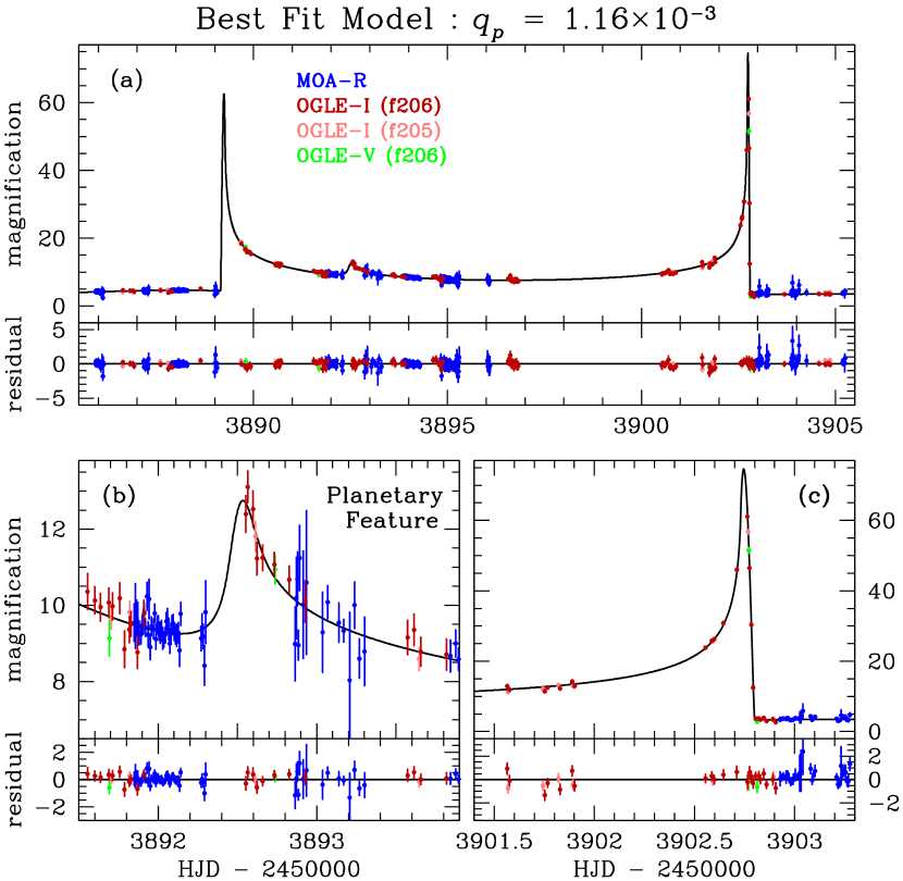
Figure 1: The best triple lens model for the OGLE-2006-BLG-284 light curve. The MOA-red data are shown in blue while the OGLE $I$-band data from fields BLG206 and BLG205 are shown in dark and light red, respectively. The OGLE $V$-band data from field BLG206, is shown in green. The solid line is the best fit model. Panel (a) shows the magnified region of the stellar binary light curve, and panels (b) and (c) show close-ups of the planetary feature and the binary caustic exit resolved by OGLE that enable the measurement of the source radius crossing time, $t_{*}$.

The second step was to fix the binary lens parameters and search for a triple lens model that could account for the feature at $3892<t<3893.5$ in the light curve (see Figure 1). (We define our time parameter as the modified Heliocentric Julian Day, $t={\rm HJD}-2450000$.) This analysis led to a number of possible solutions that maintained basically the same light curve away from this short duration anomaly. Close-ups of this short duration light curve anomaly for the three best triple lens light curve solutions are shown in Figure 3.

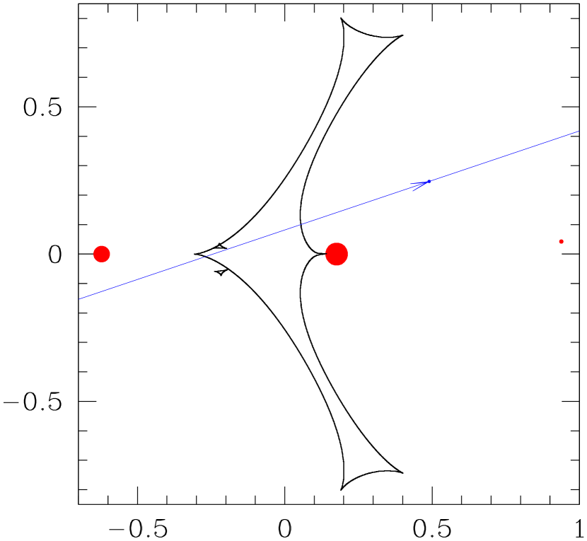
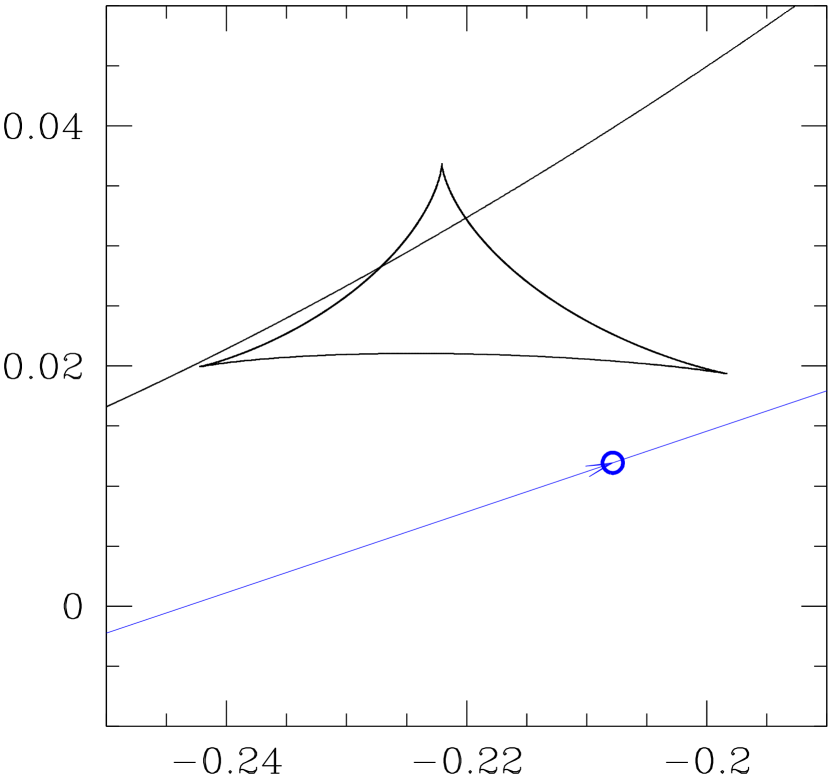
Figure 2: The caustic configuration for the best fit model is plotted in units of the Einstein radius. The line with the arrow represents the motion of the center of the source star, and the blue line and circle indicates the trajectory and size of the source star. The red dots in the right panel indicate the positions of the lens stars and planet. The close-up of the top planetary caustic in the right panel indicates that the planetary caustic overlaps with the stellar binary caustic, but has no clear interaction with it due to the fact that the caustics are related to distinct, different images.

The best fit model, shown in Figure 1, has a planetary cusp approach at ${\rm HJD}-2450000=t=3892.5$. The caustic structure for this lens system is shown in Figure 2, and it is somewhat unusual for a triple lens system because the planetary caustic crosses the stellar binary caustic with no interaction with it, although Daněk & Heyrovský (2015, 2019) have shown some examples like this. This is because the caustics affect different images. (There are 4 images when the source is outside all the caustics, 6 images when the source is inside one caustic, and 8 images when it is inside two caustic curves.) The parameters of the best fit model shown in Figure 1, as well as the two best planetary caustic crossing models, are given in Table 1. The parameters that these model has in common with a single lens model are the Einstein radius crossing time, $t_{E}$, and the time, $t_{0}$, and distance, $u_{0}$, of closest approach between the lens center-of-mass and the source star. We use the triple lens parameter system of the first published triple lens system (Gaudi et al., 2008; Bennett et al., 2010), with one minor modification. We use the mass ratios to the primary star instead of mass fractions of the total lens system mass. For this event, we assign the primary star to be mass 3, the secondary star to be mass 1, and the planet to be mass 2. The two mass ratio parameters are then $q_{1}$ for the secondary star, and $q_{2}$ for the planet. The separation between masses 2 and 3 is given by $s_{23}$ and the separation between mass 1 and the center of mass for masses 2 and 3 is given by $s_{1\rm cm}$. The angle between the source trajectory and the axis connecting mass 1 with the center-of-mass for masses 2 and 3 is given by $\alpha_{1\rm cm}$, and the angle between this axis and the line connecting masses 2 and 3 is given by $\phi_{23}$. The final lens model parameters are the source radius crossing time, $t_{*}$, and the $I$ and $V$ band source magnitudes, $I_{S}$ and $V_{S}$. The length parameters, $u_{0}$, $s_{1\rm cm}$ and $s_{23}$, are normalized by the Einstein radius of the total lens system mass, $R_{E}=\sqrt{(4GM/c^{2})D_{S}x(1-x)}$, where $x=D_{L}/D_{S}$ and $D_{L}$ and $D_{S}$ are the lens and source distances, respectively. ($G$ and $c$ are the Gravitational constant and speed of light, as usual.)

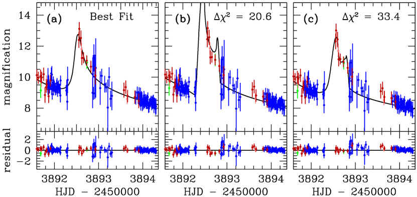
Figure 3: Comparison of the planetary features for the 3 best 2-star plus 1-planet models. The planetary feature in the best fit model, which has a planetary cusp approach feature is shown in panel (a). Panels (b) and (c) show the second and third best models which feature planetary caustic crossings. The parameters of these models are given in Table 1.

Table 1: Best Model Parameters

parameter	units	best fit	caustic-1	caustic-2	MCMC averages
$t_{E}$	days	39.677	39.872	39.969	$39.38\pm 0.97$
$t_{0}$	${\rm HJD}-2453800$	99.4440	99.4060	99.2922	$99.425\pm 0.066$
$u_{0}$		0.077523	0.079517	0.081596	$0.0776\pm 0.0020$
$s_{1\rm cm}$		0.79801	0.79856	0.79881	$0.8007\pm 0.0091$
$s_{23}$		0.76396	0.78233	0.78404	$0.7615\pm 0.0063$
$\alpha_{1\rm cm}$	radians	0.32432	0.33979	0.35519	$0.3237\pm 0.0039$
$\phi_{23}$	radians	0.05590	0.02075	-0.02990	$0.0607\pm 0.0093$
$q_{1}$		0.28445	0.27180	0.27395	$0.289\pm 0.011$
$q_{2}$	$10^{-4}$	11.632	4.2933	0.71234	$12.6\pm 1.9$
$t_{\ast}$	days	0.03367	0.03321	0.03311	$0.03372\pm 0.00030$
$I_{s}$		20.007	20.012	19.998	$19.995\pm 0.036$
$V_{s}$		21.815	21.827	21.807	$21.803\pm 0.036$
fit $\chi^{2}$		12414.60	12435.16	12447.96
for 12407	d.o.f.

For every passband, there are two parameters to describe the unlensed source brightness and the combined brightness of any unlensed “blend” stars that are superimposed on the source. Such “blend” stars are quite common because microlensing is only seen if the lens-source alignment is $\lower 2.15277pt\hbox{$\;\buildrel<\over{\sim}\;$}\theta_{E}\lower 2.15277pt\hbox{$\;\buildrel<\over{\sim}\;$}1\,$mas, while stars are unresolved in ground based images if their separation is $\lower 2.15277pt\hbox{$\;\buildrel<\over{\sim}\;$}1^{\prime\prime}$. These source and blend fluxes are treated differently from the other parameters because the observed brightness has a linear dependence on them, so for each set of nonlinear parameters, we can find the source and blend fluxes that minimize the $\chi^{2}$ exactly, using standard linear algebra methods (Rhie et al., 1999).

The MOA data immediately after the planetary light curve feature at $t\simeq 3892.6$ are crucial for excluding caustic crossing planetary models that would have a caustic exit at $3893.0<t<3893.5$, and the best remaining planetary caustic crossing models are the second and third best models with planetary features shown in Figures  3b and c. The $\chi^{2}$ improvement for the best fit model, shown in Figures 1 and 3a, over these competing models is relatively small, with $\chi^{2}$ improvements of $\Delta\chi^{2}=20.6$, and $\Delta\chi^{2}=33.4$ over the second and third best models (shown in Figure 3b and c), respectively. While these $\chi^{2}$ improvements are rather modest, we believe that they are sufficient to exclude these second and third best models. The best fit model is preferred by both the OGLE and MOA data sets. The $\chi^{2}$ difference between the second best fit model and the best fit model is occurs primarily at $3892<t<3895$, while the $\chi^{2}$ difference between the third best and best fit models occurs primarily at $3893<t<3896$. Both the second and third best models have planetary caustic exit features that the data has no indication. For the second best model (Figure 3b), the caustic exit is mostly squeezed between two data points, but it does get a modest $\chi^{2}$ penalty because the caustic exit feature is a bit wider than the gap between the data points at $t=3893.73$ and $t=3893.83$. Similarly, this model also has strong caustic entrance just after the last MOA data point of the previous night at $t=3892.299$. The timing of these two caustic features requires rather unlikely coincidences, so this lends credence to the idea that the best fit model is the correct one. The third best model (Figure 3c) has such a weak planetary caustic exit that it does not get a significant $\chi^{2}$ penalty, although the data also provide no caustic exit signal. Both the second and third best models predict a lower magnification than is observed in the time after these planetary caustic exits, $3892.86<t<3895$, and the data in this range contribute substantially to the $\chi^{2}$ differences between these two models and the best fit model. Because these competing models have additional circumstantial evidence against them, we are comfortable in treating their likelihood with the Gaussian probability, $e^{-\Delta\chi^{2}/2}$, in the analysis that follows.

In addition to triple lens models, we also searched for binary source, binary lens models, sometimes referred to as 2L2S models. The best 2L2S model we found has a $\chi^{2}$ larger than our best triple lens (3L1S) model by $\Delta\chi^{2}=552.56$. This is not surprising because it would require a much fainter second source to explain the low amplitude feature that we attribute to the planet as a feature due to the stellar binary. However, if the second source is much fainter than the primary, then it should also be much redder, but a much redder source would cause a shift in the MOA-red data and a large shift in the OGLE $V$ band data with respect to the OGLE $I$ band data at the time of the feature that we attribute to the planet. Therefore, we will not consider these models further.

4 Photometric Calibration and Source Radius

The light curve models listed in Table 1 constrain the finite source size through measurement of the source radius crossing time, $t_{*}$, and this allows us to derive the angular Einstein radius, $\theta_{E}=\theta_{*}t_{E}/t_{*}$, if we know the angular size of the source star, $\theta_{*}$. This can be derived from the extinction corrected brightness and color of source star (Kervella et al., 2004; Boyajian et al., 2014).

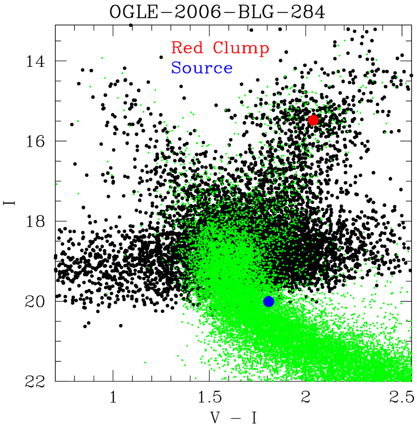
Figure 4: The $(V-I,I)$ color magnitude diagram (CMD) of the OGLE-III stars within $90^{\prime\prime}$ of OGLE-2006-BLG-284 transformed to calibrated Johnson $V$ and Cousins $I$ using the transformation given by Szymański et al. (2011). The red spot indicates red clump giant centroid, and the blue indicates the source magnitude and color. The green dots represent the HST Baade’s Window CMD of Holtzman et al. (1998) transformed to the extinction and Galactic longitude appropriate for this field.

In order to estimate the source radius, we need extinction-corrected magnitudes, which can be determined from the magnitude and color of the centroid of the red clump giant feature in the CMD (Yoo et al., 2004), as indicated in Figure 4. We find that the red clump centroid in this field is at $I_{\rm cl}=15.48$, $(V-I)_{\rm cl}=2.04$, which implies $V_{\rm cl}=17.52$. From Nataf et al. (2013), we find that the extinction corrected red clump centroid should be at $I_{\rm cl,0}=14.39$, $(V-I)_{\rm cl0,}=1.06$, which implies $I$ and extinctions of $A_{I}=1.09\pm 0.05$ and a color excess of $E(V-I)=0.098\pm 0.03$. So, the extinction corrected source magnitude and color are $I_{s0}=18.905$ and $(V-I)_{s0}=0.828$ for the average model from our MCMC calculations reported in Table 1. These dereddened magnitudes can be used to determine the angular source radius, $\theta_{*}$. With the source magnitudes that we have measured, the most precise determination of $\theta_{*}$ comes from the $(V-I),I$ relation. We use

$$\log_{10}\left[2\theta_{*}/(1{\rm\mu as})\right]=0.501414+0.419685\,(V-I)_{s0}-0.2\,I_{s0}\ ,$$ (1)

which comes from the Boyajian et al. (2014) analysis, but with the color range optimized for the needs of microlensing surveys. These numbers were provided in a private communication from T.S. Boyajian (2014). Therefore, we handle this uncertainty in our MCMC calculations, so as to include all the correlations in our determination of the lens system properties. For the average model parameters from our MCMC calculation, listed in Table 1, we find $\theta_{*}=0.585\pm 0.029\,\mu$as.

Figure 4 also includes the location of the source star on the CMD, in blue, and the Hubble Space Telescope $V$ and $I$ band CMD from Holtzman et al. (1998) after it has been shifted to the average distance and extinction of the red clump stars in the OGLE-2006-BLG284 field. The position of the source star in Figure 4 indicates that it is on the red edge of the main sequence. However, the CMD is likely to have a larger dispersion in the field of this event, due to the higher extinction in this field.

5 Lens System Properties

Table 2: Physical Parameters

Parameter	units	Value	2-$\sigma$ range
$\theta_{E}$	mas	$0.681\pm 0.035$	0.612-0.750
$\mu_{\rm rel,G}$	mas/yr	$6.31\pm 0.33$	5.66-6.97
$D_{S}$	kpc	$8.6\pm 1.2$	6.2-10.7
$D_{L}$	kpc	$4.0\pm 1.5$	1.2-6.5
$M_{L1}$	$M_{\odot}$	$0.35^{+0.30}_{-0.20}$	0.06-0.84
$M_{L2}$	$M_{\odot}$	$0.100^{+0.097}_{-0.056}$	0.018-0.24
$m_{p}$	${M_{\oplus}}$	$144^{+137}_{-82}$	25-375
$a_{\perp,ss}$	AU	$2.06\pm 0.74$	0.61-3.33
$a_{\perp,s1p}$	AU	$2.17\pm 0.78$	0.65-3.51
$V_{L}$	mag	$26.4^{+1.8}_{-2.4}$	22.3-37.2
$I_{L}$	mag	$22.9^{+1.1}_{-1.6}$	20.2-31.0
$K_{L}$	mag	$19.7^{+0.7}_{-1.0}$	17.8–26.8

Note. — Mean values and RMS are given for $\theta_{E}$, $\mu_{\rm rel,G}$, $D_{S}$, $D_{L}$, $a_{\perp,ss}$, and $a_{\perp,sp}$. Median values and 68.3% confidence intervals are given for the other parameters. 2-$\sigma$ range refers to the central 95.3% confidence interval.

With our determination of $\theta_{*}$ from the source magnitude and color in Section 4, we can now proceed to determine the lens system properties. The angular Einstein radius is given by $\theta_{E}=\theta_{*}t_{E}/t_{*}$, which allows us to use the following relation (Bennett, 2008; Gaudi, 2012)

$$M_{L}={c^{2}\over 4G}\theta_{E}^{2}{D_{S}D_{L}\over D_{S}-D_{L}}=0.9823\,M_{\odot}\left({\theta_{E}\over 1\,{\rm mas}}\right)^{2}\left({x\over 1-x}\right)\left({D_{S}\over 8\,{\rm kpc}}\right)\ ,$$ (2)

where $x=D_{L}/D_{S}$ to determine the relationship between the lens system mass, $M_{L}$ and distance, $D_{L}$. We know that the source is very likely to be approximately at the distance of the Galactic bulge, but the bulge is bar shaped and pointed at approximately the location of our Solar system. As a result, there is an uncertainty of a few kpc in the distance to the source star, $D_{S}$. Also, the probability of the lens system mass and distance also depend on the the Geocentric lens-source relative proper motion, which can be determined from the angular source size, the source angular radius, and the source radius crossing time $\mu_{\rm rel,G}=\theta_{*}/t_{*}$. We can combine all these factors with a Galactic model prior to determine our best estimate of the properties of this binary star plus planet system. We use the Galactic model of Bennett et al. (2014), and we assume that the planet hosting probability is independent of the planet mass, because this is the simplest assumption to make. We also include the 2nd and third best models in our collection of MCMC models to combine with the Galactic prior, but we weight them by $e^{-\Delta\chi^{2}/2}$, which gives them very little weight.

The results are presented in Figure 5 and Table 2. This table and figure introduce some new parameters. The primary and secondary stellar masses are given by $M_{L1}$ and $M_{L2}$, and the planet mass is $m_{p}$. Table 2 reports the projected separations, $a_{\perp,ss}$ and $a_{\perp,s1p}$, between the two stars, and between the primary star and planet, respectively. Instead of these projected separations, Figure 5, shows the predicted distribution of 3-dimensional separations, under the assumption of random orientations. However, the orientations of the primary-secondary stellar separation and the primary star-planet separations cannot be random. They must be anti-correlated in order to obey orbital stability requirements (Holman & Wiegert, 1999). For a circumstellar planet orbiting the primary star, with the observed secondary-primary mass ratio of $0.289\pm 0.011$, the semi-major axis of the planet must be $\leq 0.38$ times the semi-major axis of the stellar binary system, if we assume that both orbits are nearly circular. In the circumbinary case, Holman & Wiegert (1999) find that the planet must have a semi-major axis $\geq 2.2$ times the semi-major axis of the stellar binary system, assuming nearly circular orbits. Since the observed separations in Table 2 are nearly identical, this implies that the 3-dimensional separation of either the primary star and the planet or the two planets must be $\geq 2.2$ times the projected separations.

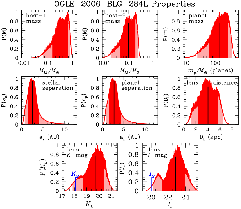
Figure 5: The lens properties from our Bayesian analysis. Host-1 and Host-2 are the primary and secondary stars of the system. The stellar and planetary separations are the separations from the primary star. The blue lines in the bottom two panels indicate the source magnitudes.

The bottom two panels of Figure 5 have blue lines that indicate the magnitudes of the combined light from both source stars as vertical blue lines. In June, 2020, it will be 14 years since this event has occurred, so the lens-source separation should be $>88.3\pm 4.6\,$mas after June 2020. Our experience with Keck adaptive optics observations (Bennett et al., 2020; Bhattacharya et al., 2020; Terry et al., 2020) indicates that the lens should be detectable at this separation if it is within 3 magnitudes of the source brightness, and our Bayesian analysis indicates that there is a 96.4% chance that the lens system is $\leq 3\,$mag fainter than the source stars.

6 Conclusions

Our analysis of OGLE-III data from two fields and MOA data from the MOA 9-year retrospective analysis for microlensing event OGLE-2006-BLG-284 has revealed that this event is due to a triple lens system consisting of two stars and a planet. While there are two light curve models with $\chi^{2}$ values that are only $\Delta\chi^{2}=20.6$ and 33.4 higher than the best fit solution, we argue that these also have very unlikely parameters. And we do not consider these to be possible solutions for this event.

The prime stumbling block for the interpretation of this event is the fact that the projected separation of the primary and secondary stars is nearly identical to the projected separation between the planet and the primary star. Thus, we cannot tell from the light curve data alone whether planet orbits both stars (circumbinary) or only one (circumstellar). Fortunately, because the event occurred so long ago, the lens-source separation is now large enough ($\lower 2.15277pt\hbox{$\;\buildrel>\over{\sim}\;$}88\,$mas) that it should be readily detected by Keck adaptive optics observations, which has now been done for a number of host stars of microlens planets (Gaudi et al., 2008; Bennett et al., 2010, 2020; Batista et al., 2015; Beaulieu et al., 2016, 2018; Bhattacharya et al., 2018, 2020; Terry et al., 2020). This may provide an opportunity to make observations that can decide between the circumbinary and circumstellar possibilities with the next generate of large telescopes. A time series of radial velocity observations of the lens system with a precision of $\sim 2\,$km/sec should be able to detect the radial velocity of the primary star if it has a relatively small semi-major axis of $\lower 2.15277pt\hbox{$\;\buildrel<\over{\sim}\;$}2\,$AU. This would imply that two stars were in the relatively close orbit and that the planet would have to be in a much wider orbit, with a large line-of-sight separation. Conversely, the failure to detect any radial velocity for the primary lens star at the $\sim 2\,$km/sec level would imply that the primary and secondary stars have a wide orbit and the planet orbits only the primary.

The details of any radial velocity program will depend on the brightness of the lens star system, which has yet to be determined. The $K_{L}$ histogram in Figure 5 indicates that there is a 95% chance that the lens system magnitude is in the range $17.5<K_{L}<20.9$, but this also represents a range of lens system distances of $1.0\,{\rm kpc}<D_{L}<7.5\,$kpc and a primary star mass range of $0.08M_{\odot}<M_{L1}<1.05M_{\odot}$. Since the star-star and planet-star separations, as well as the orbital period, are proportional to $D_{L}$, this implies a large range of possible masses and orbital periods, as well as a 3.4 magnitude brightness range. Thus, we cannot really determine the observational effort needed to test the circumbinary vs. circumstellar interpretations until we have detected the lens star with high angular resolution imaging. Even in the most optimistic scenario with $K_{L}<18$, current telescopes and instruments are unlikely to be able to make such measurements, but there is some hope for observations with the next generation of extremely large telescopes (ELTs). However, this may require advanced instrumentation that may not be available at first light on these ELTs.

This discovery tends to confirm the Gould et al. (2014) prediction that there are likely to be many undiscovered planetary signals in the existing catalog of observed microlensing events, and it may help to reduce the deficit of planets in binary systems noted by Koshimoto et al. (2020). Such events probe a range of planets in binary systems that are difficult to explore with other methods, and so they are likely to provide a unique new window on the formation of planets in binary systems and the planet formation process, in general.

The search for planets in binary systems would benefit from more efficient triple-lens modeling methods and more efficient methods to search the triple lens parameter space. This problem will come more acute with the launch of NASA’s Wide Field Infrared Survey Telescope (WFIRST) (Spergel et al., 2015), which will devote a large fraction of its observing time to an exoplanet microlensing survey (Bennett & Rhie, 2002; Bennett et al., 2018a; Penny et al., 2019). This will provide a much larger sample of exoplanets than can be observed from the ground, and will have much better light curve sampling than any ground based survey. A more robust triple-lens modeling system will be needed to take advantage of the circumbinary and circumstellar planets that will be detectable in the WFIRST data.

References

- Alard & Lupton (1998) Alard, C. & Lupton, R.H. 1998, ApJ, 503, 325
- Batista et al. (2015) Batista, V., Beaulieu, J.-P., Bennett, D.P., et al. 2015, ApJ, 808, 170
- Beaulieu et al. (2018) Beaulieu, J.-P., Batista, V., Bennett, D. P., et al. 2018, AJ, 155, 78
- Beaulieu et al. (2016) Beaulieu, J.-P., Bennett, D. P., Batista, V., et al. 2016, ApJ, 824, 83
- Bennett (2008) Bennett, D.P, 2008, in Exoplanets, Edited by John Mason. Berlin: Springer. ISBN: 978-3-540-74007-0, (arXiv:0902.1761)
- Bennett (2010) Bennett, D.P. 2010, ApJ, 716, 1408
- Bennett et al. (2018a) Bennett, D. P., Akeson, R., Anderson, J., et al. 2018a, (arXiv:1803.08564)
- Bennett et al. (2014) Bennett, D. P., Batista, V., Bond, I. A., et al. 2014, ApJ, 785, 155
- Bennett et al. (2020) Bennett, D. P., Bhattacharya, A., Beaulieu, J.-P., et al. 2020, AJ, 159, 68
- Bennett & Rhie (1996) Bennett, D.P. & Rhie, S.H. 1996, ApJ, 472, 660
- Bennett & Rhie (2002) Bennett, D.P. & Rhie, S.H. 2002, ApJ, 574, 985
- Bennett et al. (2010) Bennett, D. P., Rhie, S. H., Nikolaev, S., et al. 2010, ApJ, 713, 837
- Bennett et al. (2016) Bennett, D.P., Rhie, S.H., Udalski, A., et al. 2016, AJ, 152, 125
- Bhattacharya et al. (2018) Bhattacharya, A., Beaulieu, J.-P., Bennett, D. P., et al. 2018, AJ, 156, 289
- Bhattacharya et al. (2020) Bhattacharya, A., et al. 2020, in preparation
- Bond et al. (2001) Bond, I. A., Abe, F., Dodd, R. J., et al. 2001, MNRAS, 327, 868
- Bond et al. (2017) Bond, I. A., Bennett, D. P., Sumi, T., et al. 2017, MNRAS, 469, 2434
- Boyajian et al. (2014) Boyajian, T.S., van Belle, G., & von Braun, K., 2014, AJ, 147, 47
- Chauvin et al. (2011) Chauvin, G., Beust, H., Lagrange, A.-M., et al. 2011, A&A, 528, A8
- Correia et al. (2008) Correia, A. C. M., Udry, S., Mayor, M., et al. 2008, A&A, 479, 271
- Daněk & Heyrovský (2015) Daněk, K., & Heyrovský, D. 2015, ApJ, 806, 99
- Daněk & Heyrovský (2019) Daněk, K., & Heyrovský, D. 2019, ApJ, 880, 72
- Doyle et al. (2011) Doyle, L. R., Carter, J. A., Fabrycky, D. C., et al. 2011, Science, 333, 1602
- Gaudi (2012) Gaudi, B. S. 2012, ARA&A, 50, 411
- Gaudi et al. (2008) Gaudi, B. S., Bennett, D. P., Udalski, A., et al. 2008, Science, 319, 927
- Gould & Loeb (1992) Gould, A. & Loeb, A. 1992, ApJ, 396, 104
- Gould et al. (2014) Gould, A., Udalski, A., Shin, I.-G., et al. 2014, Science, 345, 46
- Han et al. (2017) Han, C., Udalski, A., Gould, A., et al. 2017, AJ, 154, 223
- Hatzes et al. (2003) Hatzes, A. P., Cochran, W. D., Endl, M., et al. 2003, ApJ, 599, 1383
- Holman & Wiegert (1999) Holman, M. J., & Wiegert, P. A. 1999, AJ, 117, 621
- Holtzman et al. (1998) Holtzman, J. A., Watson, A. M., Baum, W. A., et al. 1998, AJ, 115, 1946
- Hwang et al. (2019) Hwang, K.-H., Ryu, Y.-H., Kim, H.-W., et al. 2019, AJ, 157, 23
- Ida & Lin (2004) Ida, S. & Lin, D.N.C. 2004, ApJ, 604, 388
- Jaroszyński et al. (2010) Jaroszyński, M., Skowron, J., Udalski, A., et al. 2010, Acta Astron., 60, 197
- Kaib et al. (2013) Kaib, N. A., Raymond, S. N., & Duncan, M. 2013, Nature, 493, 381
- Kervella et al. (2004) Kervella, P., Thévenin, F., Di Folco, E., & Ségransan, D. 2004, A&A, 426, 297
- Kondo et al. (2019) Kondo, I., Sumi, T., Bennett, D. P., et al. 2019, AJ, 158, 224
- Koshimoto et al. (2020) Koshimoto, N., Bennett, D. P., & Suzuki, D. 2019, AJ, in press (arXiv:1910.11448)
- Koshimoto et al. (2014) Koshimoto, N., Udalski, A., Sumi, T., et al. 2014, ApJ, 788, 128
- Kostov et al. (2014) Kostov, V. B., McCullough, P. R., Carter, J. A., et al. 2014, ApJ, 784, 14
- Kostov et al. (2013) Kostov, V. B., McCullough, P. R., Hinse, T. C., et al. 2013, ApJ, 770, 52
- Kostov et al. (2016) Kostov, V. B., Orosz, J. A., Welsh, W. F., et al. 2016, ApJ, 827, 86
- Kraus et al. (2016) Kraus, A. L., Ireland, M. J., Huber, D., et al. 2016, AJ, 152, 8
- Lissauer (1993) Lissauer, J.J. 1993, Ann. Rev. Astron. Ast., 31, 129
- Marzari & Thebault (2019) Marzari, F., & Thebault, P. 2019, Galaxies, 7, 84
- Mordasini et al. (2009) Mordasini, C., Alibert, Y., & Benz, W. 2009, A&A, 501, 1139
- Mugrauer & Neuhäuser (2009) Mugrauer, M., & Neuhäuser, R. 2009, A&A, 494, 373
- Nataf et al. (2013) Nataf, D. M., Gould, A., Fouqué, P., et al. 2013, ApJ, 769, 88
- Nayakshin et al. (2019) Nayakshin, S., Dipierro, G., & Szulágyi, J. 2019, MNRAS, 488, L12
- Nelson (2000) Nelson, A. F. 2000, ApJ, 537, L65
- Neuhäuser et al. (2007) Neuhäuser, R., Mugrauer, M., Fukagawa, M., et al. 2007, A&A, 462, 777
- Orosz et al. (2012) Orosz, J. A., Welsh, W. F., Carter, J. A., et al. 2012, Science, 337, 1511
- Paardekooper et al. (2008) Paardekooper, S.-J., Thebault, P., & Mellema, G., 2008, MNRAS, 386, 973
- Penny et al. (2019) Penny, M. T., Gaudi, B. S., Kerins, E., et al. 2019, ApJS, 241, 3
- Picogna & Marzari (2013) Picogna, G., & Marzari, F. 2013, A&A, 556, A148
- Poleski et al. (2014) Poleski R., Skowron J., Udalski A., et al., 2014, ApJ, 795, 1
- Pollack et al. (1996) Pollack, J. B., Hubickyj, O., Bodenheimer, P., et al. 1996, Icarus, 124, 62
- Rhie et al. (1999) Rhie, S. H., Becker, A. C., Bennett, D. P., et al. 1999, ApJ, 522, 1037
- Roell et al. (2012) Roell, T., Neuhäuser, R., Seifahrt, A., et al. 2012, A&A, 542, A92
- Smullen et al. (2016) Smullen, R. A., Kratter, K. M., & Shannon, A. 2016, MNRAS, 461, 1288
- Spergel et al. (2015) Spergel, D., Gehrels, N., Baltay, C., et al. 2015, arXiv:1503.03757
- Suzuki et al. (2018) Suzuki, D., Bennett, D. P., Ida, S., et al. 2018, ApJ, 869, L34
- Suzuki et al. (2016) Suzuki, D., Bennett, D. P., Sumi, T., et al. 2016, ApJ, 833, 145
- Szymański et al. (2011) Szymański, M. K., Udalski, A., Soszyński, I., et al. 2011, Acta Astron., 61, 83
- Terry et al. (2020) Terry, S., et al. 2020, in preparation
- Thebault (2011) Thebault, P., 2011, CeMDA, 111, 29
- Thebault & Haghighipour (2015) Thebault, P., & Haghighipour, N. 2015, Planetary Exploration and Science: Recent Results and Advances, 309 (arXiv:1406.1357)
- Tomaney & Crotts (1996) Tomaney, A.B. & Crotts, A.P.S. 1996, AJ112, 2872
- Udalski (2003) Udalski, A. 2003, Acta Astron., 53, 291
- Udalski et al. (2008) Udalski, A., Szymański, M., Soszyński, I. & Poleski, R. 2008, Acta Astron., 58, 69
- Udalski et al. (2018) Udalski, A., Ryu, Y.-H., Sajadian, S., et al. 2018, Acta Astron., 68, 1
- Welsh et al. (2012) Welsh, W. F., Orosz, J. A., Carter, J. A., et al. 2012, Nature, 481, 475
- Welsh et al. (2015) Welsh, W. F., Orosz, J. A., Short, D. R., et al. 2015, ApJ, 809, 26
- Yoo et al. (2004) Yoo, J., DePoy, D. L., Gal-Yam, A., et al. 2004, ApJ, 603, 139
- Zsom et al. (2011) Zsom, A., Sándor, Z., & Dullemond, C. P. 2011, A&A, 527, A10
- Zucker et al. (2004) Zucker, S., Mazeh, T., Santos, N. C., et al. 2004, A&A, 426, 695