Simpson’s paradox in Covid-19 case fatality rates:
a mediation analysis of age-related causal effects

Abstract

We point out an instantiation of Simpson’s paradox in Covid-19 case fatality rates (cfrs): comparing a large-scale study from China (17 Feb) with early reports from Italy (9 Mar), we find that cfrs are lower in Italy for every age group, but higher overall. This phenomenon is explained by a stark difference in case demographic between the two countries. Using this as a motivating example, we introduce basic concepts from mediation analysis and show how these can be used to quantify different direct and indirect effects when assuming a coarse-grained causal graph involving country, age, and case fatality. We curate an age-stratified cfr dataset with $>$750k cases and conduct a case study, investigating total, direct, and indirect (age-mediated) causal effects between different countries and at different points in time. This allows us to separate age-related effects from others unrelated to age and facilitates a more transparent comparison of cfrs across countries at different stages of the Covid-19 pandemic. Using longitudinal data from Italy, we discover a sign reversal of the direct causal effect in mid-March which temporally aligns with the reported collapse of the healthcare system in parts of the country. Moreover, we find that direct and indirect effects across 132 pairs of countries are only weakly correlated, suggesting that a country’s policy and case demographic may be largely unrelated. We point out limitations and extensions for future work, and, finally, discuss the role of causal reasoning in the broader context of using AI to combat the Covid-19 pandemic.

During a global pandemic, understanding the causal effects of risk factors such as age on Covid-19 fatality is an important scientific question. Since randomised controlled trials are typically infeasible or unethical in this context, causal investigations based on observational data—such as the one carried out in this work—will, therefore, be crucial in guiding our understanding of the available data. Causal inference, in particular mediation analysis, can be used to resolve apparent statistical paradoxes; help educate the public and decision-makers alike; avoid unsound comparisons; and answer a range of causal questions pertaining to the pandemic, subject to transparently-stated assumptions. Our exposition helps clarify how mediation analysis can be used to investigate direct and indirect effects along different causal paths and thus serves as a stepping stone for future studies of other important risk factors for Covid-19 besides age.

I Introduction

The 2019–20 coronavirus pandemic originates from the SARS-CoV-2 virus, which causes the associated infectious respiratory disease Covid-19. After an outbreak was identified in Wuhan, China, in December 2019, cases started being reported across multiple countries all over the world, ultimately leading to the World Health Organization declaring it a pandemic on 11 March 2020 [68]. As of 28 September 2020, the pandemic led to more than 33 million confirmed cases and one million fatalities across 188 countries [32]. One of the most cited indicators regarding Covid-19 is the reported case fatality rate (cfr), which indicates the proportion of confirmed cases which end fatally. In addition to the total cfr, cfrs are often also reported separately by age since cfrs differ significantly across different age groups, with older people statistically at higher risk.

In this work, we show how tools from causal inference and, in particular, mediation analysis can be used to interpret Covid-19 case fatality data. We motivate our investigation by pointing out what could be a textbook example of Simpson’s paradox in comparing cfrs between China and Italy, suggesting opposite conclusions depending on whether the data is analysed in aggregate or age-stratified form (section II). This example illustrates how a traditional statistical analysis provides insufficient understanding of the data, and thus needs to be augmented by additional assumptions about the underlying causal relationships. In section III, we therefore postulate a coarse-grained causal model for comparing age-specific Covid-19 cfr data across different countries. We then review different types of (direct and indirect) causal effects, and motivate them in the context of our assumed model as different questions about Covid-19 case fatality in section IV.

Figure 1: (left) Covid-19 case fatality rates (cfrs) in Italy and China by age group and in aggregated form (“Total”), i.e., incl. all confirmed cases and fatalities up to the time of reporting (see legend). (right) Proportion of cases within each age group.

As one of our contributions, we curated a dataset involving 756,004 confirmed Covid-19 cases and 68,508 fatalities, separated into age groups of 10-year intervals (0–9, 10–19, etc.), reported from 11 different countries from Africa, Asia, Europe and South America and the Diamond Princess cruise ship, which, together with an interactive notebook containing all our analyses, is publicly available. We use this dataset, in combination with the proposed coarse-grained model, to perform a case study (section V). Tracing the evolution of direct and indirect age-mediated effects of country (China or Italy) on case fatality from early March to late May 2020 allows to discover trends that may otherwise remain hidden in the data, e.g., a reversal in the sign of the direct effect in mid March that temporally aligns with a reported “collapse” of the health-care system in parts of Italy [2]. Moreover, we compute direct and indirect effects for 132 pairs of countries and thus identify countries whose total cfrs are particularly adversely affected by their case demographic. We further find that indirect (age-related) effects are strongly correlated with a country’s population’s median age, but only weakly with direct effects.

Due to the limited availability of age-stratified fatality data, our model is relatively simple, and we do not claim novelty in the causal methodology. However, this work constitutes, to the best of our knowledge, the first application of causal analysis to better understand the role of mediators such as age in the context of Covid-19. While the use of cfr data may be problematic due to selection bias from differences in testing (which we discuss in section VI), we emphasise that our causal framework may likewise be applied to more comprehensive datasets once available. We thus hope that our work can serve as a stepping stone for further studies to gain better insight into the mechanisms underlying Covid-19 fatality using a principled and transparent causal framework.

II Simpson’s paradox in comparing cfrs between China and Italy

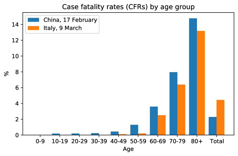
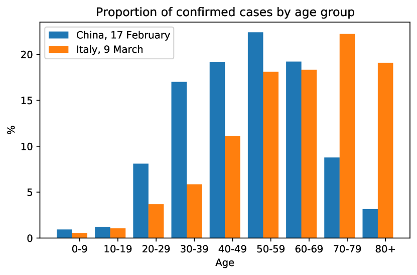
When comparing Covid-19 cfrs for different age groups (i.e., the proportion of confirmed Covid-19 cases within a given age group which end fatal) reported by the Chinese Center for Disease Control and Prevention [70] with preliminary cfrs from Italy as reported on March 9 by the Italian National Institute of Health [29] a surprizing pattern can be observed: for all age groups, cfrs in Italy are lower than those in China, but the total cfr in Italy is higher than that in China. This is illustrated in Fig. 1—see Appendix -D for exact numbers. It constitutes a textbook example of a statistical phenomenon known as Simpson’s paradox (or reversal) which refers to the observation that aggregating data across subpopulations (here, age groups) may yield opposite trends (and thus lead to reversed conclusions) from considering subpopulations separately [63].

How can such a pattern be explained? The key to understanding the phenomenon lies in the fact that we are dealing with relative frequencies: the cfrs shown in percent in Fig. 1 (left) are ratios and correspond to the conditional probabilities of fatality given a case from a particular age group and country. However, such percentages conceal the absolute numbers of cases within each age group. Considering these absolute numbers sheds light on how the phenomenon can arise: the distribution of cases across age groups differs significantly between the two countries, i.e., there is a statistical association between the country of reporting and the case demographic. In particular, Italy recorded a much higher proportion of confirmed cases in older patients, as illustrated in Fig. 1 (right).

While most cases in China fell into the age range of 30–59, the majority of cases reported in Italy were in people aged 60 and over who are generally at higher risk of dying from Covid-19 ​​, as illustrated by the increase in cfrs with age for both countries. The observed difference may partly stem from the fact that the Italian population in general is older than the Chinese one with median ages of 45.4 and 38.4 respectively, but additional factors such as different testing strategies and patterns in the social contacts among older and younger generations [e.g., 41, 54, 74] may also play a role. In summary, the larger share of confirmed cases among elderly people in Italy, combined with the fact that the elderly are generally at higher risk when contracting Covid-19 ​​, explains the mismatch between total and age-stratified cfrs and thus gives rise to Simpson’s paradox in the data.

We note that other instances of Simpson’s paradox have already been observed in the context of epidemiological studies. When recording tubercolosis deaths in New York City and Richmond, Virginia in 1910, for example, it was noted that, even though overall tubercolosis mortality was lower in New York than in Richmond, the opposite was true when populations where stratified according to ethnicity [16].

III A causal model for Covid-19 cfr data

While the previous reasoning provides a perfectly consistent explanation in a statistical sense, the phenomenon may still seem puzzling as it defies our causal intuition—similar to how an optical illusion defies our visual intuition. Humans appear to naturally extrapolate conditional probabilities to read them as causal effects, which can lead to inconsistent conclusions and may leave one wondering: how can the disease in Italy be less fatal for the young, less fatal for the old, but more fatal for the people overall? It is for this reason of ascribing causal meaning to probabilistic statements, that the reversal of (conditional) probabilities in section II is perceived as and referred to as a “paradox”  [47, 48, 27].

The aspiration to extract causal conclusions from data is particularly strong during a pandemic, when many inherently causal questions are naturally asked. For example, politicians and citizens may want to evaluate different strategies to fight the disease by asking interventional or counterfactual (”what would have happened if …?”) questions. However, it is a well-known scientific mantra that correlation does not imply causation, and observational data (like that in Fig. 1) alone is generally insufficient to draw causal conclusions. While correlations can be seen as a result of underlying causal mechanisms [56], different causal models can explain the same statistical association patterns equally well [46]. Additional assumptions on the underlying causal structure are therefore necessary to guide reasoning based on observational data.

III-A Included Variables

We consider the following three variables for comparing Covid-19 cfrs across different countries:

1. the country $C$ in which a confirmed case is reported, modelled as a categorical variable;

2. the age group $A$ of a positively-tested patient, an ordinal variable with 10-year intervals as values;

3. the medical outcome, or fatality, $F$, a binary variable indicating whether a patient has deceased by the time of reporting ($F=1$) or not ($F=0$).

III-B Data Generating Process and Causal Graph

We assume the causal graph shown in Fig. 2, motivated by thinking of the following data-generating process:

1. Choosing a country $C$ at random;

2. Given the selected country $C$, sampling a positively-tested patient with age group $A$;

3. Conditional on the choice of $C$ and $A$, sampling the case fatality $F$.

This is clearly a very simple and coarse-grained view of what is known to be a complex underlying phenomenon. As a consequence, we abstract away various influences and mechanisms within the arrows in Fig. 2.

Figure 2: Assumed causal graph: within this view age $A$ acts as a mediator of the effect of country $C$ on case fatality $F$.

• $(C\rightarrow A)$ captures that the case demographic is country-dependent. This difference might be due to a general difference in age demographic between countries, but other mechanisms such as inter-generational mixing or age-targeted social distancing may also play a role.

• $(A\rightarrow F)$ encodes that Covid-19 is more dangerous for the elderly: age seems to have a causal effect on fatality.

• $(C\rightarrow F)$ summarises country-specific influences on case fatality other than age, e.g., medical infrastructure such as availability of hospital beds and ventilators, local expertise and pandemic-preparedness (e.g., from experience with SARS), air pollution levels, and other non-pharmaceutical interventions and policies which may indirectly affect case fatality via caseload, influencing the capacity of the healthcare system. We will refer to the combination of all these effects as a country’s approach.

We emphasise that we do not explicitly model the infection process, but consider only drivers of fatality conditional on having tested positive, see section VI for further discussion.

A similar causal model to that in Fig. 2 (see [67]) was subsequently used to assay another instance of Simpson’s paradox in Covid-19 cfr data: in that case, ethnicity rather than country of origin takes the role of a common cause of age group and fatality, and age that of a mediator [39].

III-C Observational Sample and Causal Sufficiency

We assume that cfrs and case demographic are based on an observational sample and thus constitute estimates of $P(F=1|A=a,C=c)$ and $P(A=a|C=c)$, respectively. In addition, we assume causal sufficiency, meaning that all common causes of $C,A,F$ are observed (i.e., there are no hidden confounders). While this is a strong assumption, it is necessary to reason about causal effects and also perhaps not entirely unrealistic in our setting: all unobserved variables described above can be seen as latent mediators.

IV Total, direct, and indirect (age-mediated) causal effects on case fatality

Having clearly stated our assumptions, we can now answer causal queries within the model postulated in section III. In this section, we review definitions of different causal effects (following the treatment of [45]) and provide interpretations thereof by phrasing them as questions about different aspects of the cfr data in Fig. 1. We defer a discussion of issues such as identifiability under different conditions to Appendix -A. Example calculations for each defined quantity using the data from Fig. 1 can be found in Appendix -B. Throughout, we denote an intervention that externally fixes a variable $X$ to a particular value $x$ (as opposed to conditioning on it) using the notation $do(X=x)$ [46].

IV-A Total Causal Effect (tce)

First, we may ask about the overall causal effect of the choice of country on case fatality:

$Q_{\textsc{tce}}$: “What would be the effect on fatality of changing country from China to Italy?”

The answer is called the average total causal effect (tce):

Definition 1 (tce).

The tce of a binary treatment $T$ on $Y$ is defined as the interventional contrast

$$\textsc{tce}_{0\rightarrow 1}= \mathbb{E}_{Y|do(T=1)}[Y|do(T=1)]$$

$$-\mathbb{E}_{Y|do(T=0)}[Y|do(T=0)].$$ (1)

In our setting (i.e., according to the causal graph in Fig. 2), the country $C$ takes the role of a treatment that affects the medical outcome $F$ (denoted by $T$ and $Y$ in Defn.1, respectively), and (subject to causal sufficiency) the tce is simply given by the difference in total cfrs.

IV-B “Why?”: Beyond Total Effects via Mediation Analysis

While computing the tce is the principled way to quantify the total causal influence, it does not help us understand what drives a difference between two countries, i.e., why it exists in the first place: we may also be interested in the mechanisms which give rise to different cfrs observed across countries. Since the age of patients was crucial for explaining the instance of Simpson’s paradox in section II, we now seek to better understand the role of age as a mediator of the effect of country on fatality. This seems particularly relevant from the perspective of countries, which—unable to influence the age distribution of the general population—only have limited control over the case demographic and thus may wish to factor out age-related effects. However, such potential mediators are not reflected within the tce, as evident from the absence of the age variable $A$ from (1).

The country $C$ causally influences fatality $F$ along two different paths: a direct path $C\rightarrow F$, giving rise to a direct effect; and an indirect path $C\rightarrow A\rightarrow F$ mediated by $A$, giving rise to an indirect effect. The tce of $C$ on $F$ thus comprises both direct and indirect effects. Quantifying such direct and indirect effects is referred to as mediation analysis [45]. The main challenge is that any changes to the country $C$ propagate along both direct and indirect paths, making it difficult to isolate the different effects. The key idea is therefore to let changes propagate only along one path while controlling or fixing the effect along the other.

IV-C Controlled Direct Effect (cde)

The simplest way to measure a direct effect is by changing the treatment (country) while keeping the mediator fixed at a particular value. For example, we may ask about the causal effect for a particular age group such as 50–59 years olds:

$Q_{\textsc{cde}(50-59)}$: “For 50–59 year-olds, is it safer to get the disease in China or in Italy?”

Because it involves actively controlling the value of the mediator, the answer to such a query is referred to as the average controlled direct effect (cde). It is defined as follows.

Definition 2 (cde).

The cde of a binary treatment $T$ on an outcome $Y$ with mediator $X=x$ is

$$\textsc{cde}_{0\rightarrow 1}(x)= \mathbb{E}[Y|do(T=1,X=x)]$$

$$-\mathbb{E}[Y|do(T=0,X=x)].$$ (2)

For our assumed setting, the cde is given by the difference of cfrs for a given age group. A practical shortcoming of the cde is that it is often difficult or even impossible to control both the treatment and the mediator. Another problem is that the cde does not provide a global quantity for comparing baseline and treatment: in our setting, there is a different cde for each age group. However, we may instead want to measure a direct effect at the population level.

IV-D Natural Direct Effect (nde)

Instead of fixing the mediator to a specific value (selecting a particular age group), we can consider the hypothetical question of what would happen under a change in treatment (country) if the mediator (age) kept behaving as it would under the control, i.e., as if the change only propagated along the direct path. This corresponds to asking about the effect of switching country without affecting the age distribution across confirmed cases.

$Q_{\text{NDE}}$: “For the Chinese case demographic, would the Italian approach have been better?”

As it relies on the mediator (age) distribution under the control (China) to evaluate the treatment (approach), the answer to $Q_{\textsc{nde}}$ is known as average natural direct effect (nde).

Definition 3 (nde).

The nde of a binary treatment $T$ on an outcome $Y$ mediated by $X$ is given by

$$\textsc{nde}_{0\rightarrow 1}=\mathbb{E}[Y_{X(0)}|do(T=1)]-\mathbb{E}[Y|do(T=0)].$$ (3)

where $X(0)$ refers to the counterfactual of $X$ had $T$ been 0.

IV-E Natural Indirect Effect (nie)

For isolating the indirect effect that a country exhibits on case fatality only via age, $C\rightarrow A\rightarrow F$, we run into the additional complication that it is not possible to keep the influence along $C\rightarrow F$ constant under a change in country. To overcome this problem, one can consider a hypothetical change in the distribution of the mediator (age) as if the treatment (country) were changed, but without actually changing it. E.g., we may ask:

$Q_{\textsc{nie}}$: “How would the overall cfr in China change if the case demographic had instead been that from Italy, while keeping all else (i.e., cfr’s of each age group) the same?”

Since this considers a change of the mediator (age) to the natural distribution it would follow under a change treatment (case demographic from Italy) while keeping the treatment the same (Chinese cfr’s), the answer to this question is referred to as the average natural indirect effect (nie).

Definition 4 (nie).

The nie of a binary treatment $T$ on an outcome $Y$ with mediator $X$ is given by

$$\textsc{nie}_{0\rightarrow 1}=\mathbb{E}[Y_{X(1)}|do(T=0)]-\mathbb{E}[Y|do(T=0)].$$ (4)

IV-F Mediation Formulas

For causally sufficient systems, the interventional distributions of each variable given its causal parents equal the corresponding observational distributions, reflecting the intuition that they represent mechanisms rather than mere mathematical constructs [52]. tce (1) and cde (2) then reduce to:

$$\textsc{tce}^{\text{obs}}_{0\rightarrow 1}= \mathbb{E}[Y|T=1]-\mathbb{E}[Y|T=0],$$ (5)

$$\textsc{cde}^{\text{obs}}_{0\rightarrow 1}(x)= \mathbb{E}[Y|T=1,X=x]-\mathbb{E}[Y|T=0,X=x].$$ (6)

Moreover, in this case, nde (3) and nie (4) are given by the following mediation formulas [45]:

$$\textsc{nde}^{\text{obs}}_{0\rightarrow 1}= \textstyle\sum_{x}P\big{(}X=x|T=0\big{)}\big{(}\mathbb{E}[Y|T=1,X=x]$$

$$-\mathbb{E}[Y|T=0,X=x]\big{)},$$ (7)

$$\textsc{nie}^{\text{obs}}_{0\rightarrow 1}= \textstyle\sum_{x}\big{(}P(X=x|T=1)$$

$$-P(X=x|T=0)\big{)}\mathbb{E}[Y|T=0,X=x].$$ (8)

When comparing cfrs across countries, we only have observational data and thus rely on causal sufficiency (section III) to compute total, direct and indirect effects via (5), (6) (IV-F), (IV-F).

IV-G Relation between tce, nde, and nie

Can the total causal effect be decomposed into a sum of direct and indirect contributions? While such an additive decomposition indeed exists for linear models, it does not hold in general due to possible interactions between treatment and mediator, referred to as moderation. Direct and indirect effects are not uniquely defined in general, but depend on the value of the mediator. Counterfactual quantities such as nde and nie are thus useful tools to measure some average form of direct and indirect effect with a meaningful interpretation.

IV-H Mediation analysis in AI: algorithmic fairness

While the present work is focused on the study of Covid-19 cfrs, we remark that the ideas and tools of causal mediation analysis presented in this section also feature prominently in other areas of AI, e.g., in the field of algorithmic fairness which aims to uncover and correct for discriminatory biases of models. In this context, discrimination is often interpreted as a causal influence of a protected attribute (such as age, sex, ethnicity, etc) on an outcome of interest along paths which are considered unfair for a setting at hand [33, 36, 75, 15, 69].

A historic example and a famous instance of Simpson’s paradox is the case of UC Berkeley graduate admissions [11]: in 1973, pooled data across all departments showed that a substantially larger proportion of all male applicants were admitted (44%) when compared to females (35%), suggesting gender bias. However, careful mediation analysis subsequently revealed that this difference was entirely explained by the choice of department—females generally applied to departments with lower admission rates—and that when controlling for the mediating variable “department choice,” i.e., considering the direct effect of sex on admission, there was actually a small bias in favour of women [11]. Since the indirect path mediated by department choice was not considered unfair for the admission process, no wrongdoing on behalf of the school was concluded.

V Case study: mediation analysis of age-related effects on Covid-19 CFRs

Figure 3: Evolution of tce, nde, and nie of changing country from China to Italy on total cfr over time. We compare static data from China [70] with different snapshots from Italy reported by [29]. The direct effect initially was negative, meaning that age-specific fatality in Italy was lower; however, it changes sign around mid-March when an overloaded health system in northern Italy was reported [2].

V-A Dataset

To employ the tools from mediation analysis outlined in section IV to better understand the influence of age on Covid-19 cfrs, we curated a dataset of confirmed cases and fatalities by age group (0–9, 10–19, etc.) from eleven countries (Argentina, China, Colombia, Italy, Netherlands, Portugal, South Africa, Spain, Sweden, Switzerland, South Korea) and the Diamond Princess cruise ship, on which the disease spread among passengers forced to quarantine on board [59]. The dataset includes 756,004 cases and 68,508 fatalities (total cumulative cfr of 9.06%), reported either by the different countries’ national health institutes or in scientific publications. The selection of countries is based on availability of suitable data at the time of writing. Where available, we included several reports from the same country, e.g., for Italy and Spain in weekly intervals. The data and our analysis (in form of an interactive notebook) are provided in the supplement and will be made publicly available. The exact sources and several additional figures and tables can be found in Appendices -E and -F.

V-B Tracing Causal Effects Over Time

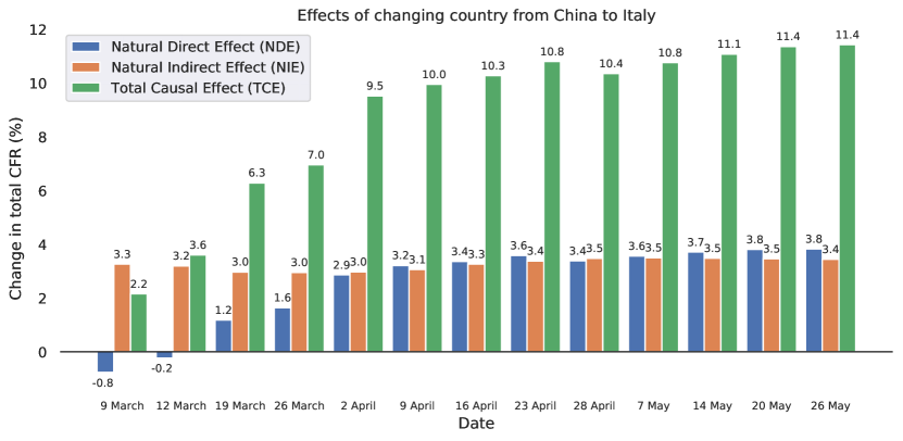
First, we investigate the temporal evolution of direct and indirect (age-mediated) causal effects on fatality by expanding on the comparison from section II. The result of tracing tce, nde, and nie of changing from China to Italy over a period of 11 weeks using (approximately) weekly reports from [29] is shown in Fig. 3. Note that case and fatality numbers for China remain constant in the figure, so any changes over time can be attributed to Italy.

We find that the tce—which measures what would happen to the total cfr if both cfrs by age group and case demographic were changed to those from Italy—is positive throughout, reflecting a higher total cfr in Italy. It increases rapidly from an initial 2.2% to 9.5% over the first three weeks considered, and then continues to rise more slowly to 11.4%. This indicates that the difference between the two countries’ total CFR becomes more pronounced over the time. In order to understand what drives this difference, we next consider the direct and indirect effects separately.

The nde—which captures what would happen to the total cfr if the case demographic were kept the same, while only the approach (cfrs per age group) were changed— is negative at first, meaning that the considered change in approach would initially be beneficial, consistent with the lower cfrs in each age group shown in Fig. 1. However, at a turning point around mid March the nde changes sign: beyond this point, switching to the Italian approach would lead to an increase in total cfr. While we can only speculate about the precise factors that came together in producing this reversal in nde, it seems worth pointing out that an overwhelmed health care system “close to collapse” in (northern) Italy was reported during that very period of early to mid-March [2]. The nde then keeps rising steeply until April before gradually flattening off, similar to the tce.

The nie—which measures what would happen to total cfr if the approach were kept the same, while the case demographic were changed to that in Italy—on the other hand, remains largely constant over time, fluctuating between 3 and 3.5%, indicating that the case demographic in Italy does not change much over time. Its large value of over 3% means that simply changing the case demographic from China to that in Italy would already lead to a substantial increase in total cfr, consistent with the larger share of confirmed cases amongst the elderly in Italy shown in Fig.  1.

In summary, while indirect age-related effects considerably contribute to differences in total cfr—especially initially, when the instance of Simpson’s paradox from section II is reflected in the opposite signs of nde and nie—it is mainly the direct effect that drives the observed changes over time.

Figure 4: ndes (left) and nies (right) for switching from the control country (columns) to the treatment country (rows). Numbers show the change in total cfr in %, i.e., negative numbers indicate that switching to the treatment country’s approach, i.e., its cfrs by age group, (nde) or case demographic (nie) would lead to a decrease in total cfr. Countries are ordered by their average effect as a treatment country (nde or nie) over the remaining 11 data points as a control.

V-C Comparison between Several Different Countries

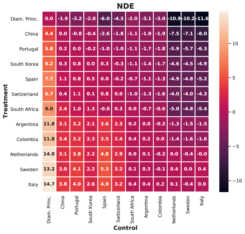
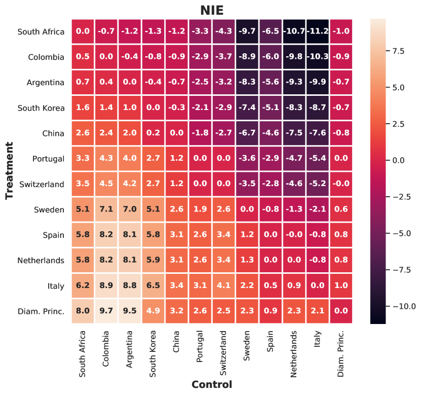
We now leave the specific example of China vs Italy aside and turn to a comparison of causal effects between the 12 countries (incl. the Diamond Princess) contained in our dataset. All pairwise effects on total cfr (in %) of changing only “approach”, i.e., the cfrs by age group, (nde; left) or case demographic (nie; right) from a control country (columns) to a treatment country (rows) are shown in Fig. 4.

For ease of visualisation, the order in which countries are presented in Fig. 4 was chosen according to their average effect as a treatment over the remaining countries as control (i.e., by the mean of rows) for nde and nie separately. This allows to read off trends about the effectiveness of different approaches and the influence of the case demographic (subject to limitations such as, e.g., differences in testing which we discuss further in section VI). In the case of nde, for example, the Diamond Princess, China, Portugal, and South Korea compare favourably to most others in terms of their approaches, while the Netherlands, Sweden, and Italy occupy the bottom end of the range. In the case of nie, South Africa, Colombia, and Argentina benefit most from their case demographic, while Spain, the Netherlands, Italy and the Diamond Princess are particularly adversely affected by it.

Notably, there is no significant correlation between countries’ ranking by nde and nie (Spearman’s $\rho=0.04$, $p=0.9$), suggesting that a country’s approach and case demographic may be largely unrelated. While some countries such as South Korea, Switzerland, the Netherlands, and Italy take almost the same place according to both rankings of particular interest are those countries for which rankings by nde and nie differ most. Other than for the Diamond Princess—which due to small sample size and high testing rates constitutes an illustrative special case that we discuss further in section VI—the case of high ranking (rk) in terms of nde and low ranking in terms of nie is most most pronounced for Spain ($\text{rk}_{\textsc{nde}}-\text{rk}_{\textsc{nie}}=-4$), Portugal ($-3$), and China ($-3$). This suggests that, for the case of Spain, the high total cfr may, at least in parts, be attributed to an unfavourable case demographic, while the approaches (age-specific fatality) of China and Portugal may be even better than suggested by their (already comparatively low) total cfrs. Conversely, countries that rank considerably higher in terms of nie than nde include Colombia ($+7$), South Africa ($+6$), and Argentina ($+5$). These countries’ low total cfrs may thus wrongly suggest a very successful approach while the low total cfr may actually, at least in parts, be due to an advantageous case demographic—again, subject to caveats such as differences in testing, see section VI for more details.

Noting that South Africa, Colombia, and Argentina are also the three youngest amongst the considered countries in terms of median age, we computed the Spearman correlation between the ranking of countries by nie and by their median age and found a strong correlation between the two ($\rho=0.94,p=7\times 10^{-6}$). This indicates that, for the countries considered, the case demographic is predominantly determined by the age distribution of the population, and suggests that countries seem not to make (effective) use of strategies such as, e.g., age-specific quarantines.

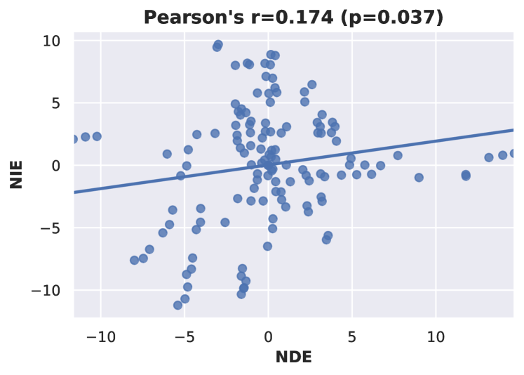
As a further investigation into the relation between direct and indirect effects on Covid-19 fatality, we find that, of the 132 ordered pairs of distinct countries, 64 exhibit opposite signs of nde and nie (as for the example of Simpson’s paradox in section II, see also dates from early March in Fig. 3), meaning that comparing countries in terms of total cfr may not give an accurate picture of the relative effectiveness of two countries’ approaches in those cases. Overall, pairwise ndes and nies are only weakly but significantly correlated (Pearson’s $r=0.17,p=0.04$), see Fig. 5.

VI Limitations and Future Work

In this work, we have taken a coarse-grained causal modelling perspective considering the variables country $C$, age group $A$, and case fatality $F$, which are reported in the context of Covid-19 cfr data. This view abstracts away many potentially important factors (some of which we named in section III) along the paths of the assumed causal graph. A strength of this approach is that it allows for consistent reasoning about age-mediated and non-age-related effects within the assumed model in situations where the data does not support a more fine-grained analysis. On the other hand, any conclusions must be interpreted within this coarse-grained view: we have thus collectively referred to various country-specific influences on fatality as “approach”.

Figure 5: Scatter plot of nie vs. nde between all 132 pairs of distinct countries: we find a weak but statistically significant positive correlation (see plot title).

VI-A Considering Additional Mediators

It is safe to assume that the virus is ultimately agnostic to the notion of different “countries” and that the influence of country on fatality $C\rightarrow F$ is not actually a direct one, but instead mediated by additional variables $X_{i}$, as illustrated in Fig. 6 (left). Candidates for such additional mediators $X_{i}$ include, e.g., non-pharmaceutical interventions and critical healthcare infrastructure. We believe that many questions of interest regarding the Covid-19 pandemic can be phrased as path-specific causal effects involving such mediators, e.g.: “What would be the effect on total cfr if country $C_{1}$ bought as many ventilators as country $C_{2}$?”. Assuming more fine-grained data will become available as the pandemic progresses, extending our model with additional mediators and investigating their effects by building on the tools described in section IV is a promising future direction to deepen our understanding about which factors most drive Covid-19 fatality.

VI-B Testing Strategy and Selection Bias

An important potential limitation of our approach (or, more fundamentally, of cfr data) is that we only consider confirmed cases, i.e., patients who tested positively for Covid-19. We can make this explicit in our model by including test status $T$ as additional variable. Our data is then always conditioned on $T=1$, as illustrated in Fig. 6 (right). Since who is tested is not random, but generally depends both on a country’s testing strategy and a patient’s age (e.g., via severity of symptoms), reflected by the arrows $\{C,A\}\rightarrow T$, this results in a problem of selection bias [55]. This issue is particularly clear for the Diamond Princess on which “3,063 PCR tests were performed among [the 3,711] passengers and crew members. Testing started among the elderly passengers, descending by age” [59]. As a result of such extensive testing, the proportion of asymptomatic cases on board was very high (318 out of 619 detected cases), leading to low cfrs as manifested in the negative ndes for the Diamond Princess as treatment in Fig. 4. This rate of testing is presently not feasible for countries with millions of inhabitants. Since testing capacities differ across countries, the reported cfrs may thus often not be comparable. Building on recent (causal) work on recoverability from selection bias may help address this aspect of the problem [4, 17].

A second source of bias may stem from the choice of countries included in our dataset: we only considered countries that report age-stratified cfrs—those might be particularly affected by the pandemic. The cumulative cfr of 9% is thus likely inflated by such selection processes. An additional problem is the delay between time of infection and death: to correct for this, fatalities should be divided by the number of patients infected at the same time as those who died, i.e., excluding the most recent cases  [8], which requires estimating the incubation period.

Figure 6: (left) The direct effect $C\rightarrow F$ is likely mediated by additional variables $X_{i}$. (right) Testing strategy may introduce selection bias, since cfr data implicitly conditions on having tested positive, represented by the shaded $T$.

VI-C cfr vs. Infection Fatality Rate

To overcome such testing and delay issues, one should ideally instead use the (delay-corrected) infection fatality rate (ifr), defined as the ratio of fatalities over all infected patients, including asymptomatic ones. However, this requires estimating the number of undetected cases based on specific modelling assumptions (which may not hold in practice, thus potentially introducing additional biases) for each country or region separately, and consequently we are only aware of very few estimates of age-stratified ifrs [e.g., 66, 58, 59]. Our analysis may be adapted for ifr data as well though, see Appendix -C for more details.

VII Discussion

The problem of case fatality rates is a compelling example of Simpson’s paradox which brings to bear a core method of AI (causal reasoning) on a Covid-19 problem. We would like to place this in a broader context by discussing (A) additional links between Simpson’s paradox and AI, and (B) contributions of AI in the ongoing pandemic.

VII-A Simpson’s paradox in the context of AI

We have above mentioned examples of Simpson’s paradox in college admission policies [11] and epidemiology [16]. In addition, it has been observed that the paradox may occur in many other real life contexts [42, 72], thus making its understanding relevant to the field of artificial intelligence, commonsense reasoning and in the study of uncertain reasoning systems in general. Furthermore, the reversal in Simpson’s paradox becomes critical in decision making situations [43, 48], where an agent needs to move beyond a merely predictive setting and reason about the effect of actions or interventions. As already discussed, the paradox can be “resolved” in different ways depending on the causal model (e.g., whether covariates take the role of confounders or mediators) and the causal query of interest to the agent (e.g., whether a direct, indirect, or total causal effect is to be estimated). If variables which are relevant for a correct resolution of the “paradox” are not directly observed, this can be particularly problematic, and causal reasoning therefore bears nontrivial conceptual and algorithmic implications, e.g., in sequential decision making contexts such as the multi-armed bandit problem (see [5, 21]).

Since Simpson’s paradox demonstrates that opposite conclusions can be reached depending on how the data is aggregated or stratified, it also has close connections to clustering [31, 73], another core AI technique, which is especially challenging for high-dimensional data as is commonplace in the age of big data. Other seemingly paradoxical reversals, related to Simpson’s paradox, can also occur in the context of games; for example, in Parrondo’s paradox, a coin flip game with a positively-biased outcome can be generated from the combination of two negatively-biased processes [23, 24].

VII-B AI against Covid-19: a causal view

Given the global disruption caused by Covid-19, there is a growing body of work trying to leverage AI and data science to help curtail and combat the ongoing pandemic, e.g., in contact tracing [1, 7], symptom screening [64], risk scoring [61], vaccine development [44], or diagnosis from CT [6] or X-ray [18] imaging—see, e.g., [38, 65, 37] for reviews. Due to typically small sample sizes and population differences, however, such applications of AI need to be critically assessed with respect to transparency and generalisability to different cohorts of individuals [25]. Indeed, a recent meta-analysis of 232 models for diagnosis, prognosis, and detection of Covid-19 concluded that “almost all published prediction models are poorly reported, and at high risk of bias such that their reported predictive performance is probably optimistic” [71].

The question whether a machine learning model will generalise outside its training distribution is closely linked to some of the concepts from causality discussed in the present work and has been studied in the causal inference literature under the term “transportability” [50, 3]. If, as is common practice, the aim is to maximise predictive performance on the available data, then any trained model is encouraged to rely on “spurious” correlations (e.g., due to unobserved confounding) which may not generalise to different populations (e.g., different countries) or modes of reasoning, such as reasoning about the outcome of treatment interventions based on observational data. Causal mechanisms, on the other hand, constitute stable (or invariant) units which are often largely independent of other components of a system and should thus be transferable even if the distribution of some features changes [60, 52]. The above reasoning cautions against blind use of supervised learning techniques without regard to the underlying causal structure. Indeed, we would argue that applications of AI techniques on Covid-19 may often benefit from formulating a causal model underlying the observed data (including potential population differences), as done in some studies [14, 10, 22].

VIII Conclusion

We have shown how causal reasoning can guide the interpretation of Covid-19 case fatality data. In particular, mediation analysis provides tools for separating effects due to different factors which, if not properly identified, can lead to misleading conclusions. We exploited these tools to uncover patterns in the time evolution of cfrs in Italy, and in the comparison of multiple countries. To study age-mediated and age-unrelated effects on cfr across different countries, we curated a large-scale dataset from a multitude of sources.

-A Additional concepts from mediation analysis

-A1 Experimental (non-)identifiability of direct and indirect effects

Since the cde in (2) only involves interventional quantities it is in principle experimentally identifiable, meaning that it can be determined through an experimental study in which both the treatment and the mediator are randomised, thus providing valid estimates of $P(Y|do(T=t,X=x))$.

In contrast, nde and nie are, in general (i.e., without further assumptions), not experimentally identifiable owing to their counterfactual nature. However, under certain conditions such non-confoundedness of mediator and outcome experimental identifiability is obtained. In this case:

$$\textsc{nde}^{\text{exp}}_{0\rightarrow 1} =\textstyle\sum_{x}P\big{(}X=x|do(T=0)\big{)}\left(\mathbb{E}[Y|do(T=1,X=x)]-\mathbb{E}[Y|do(T=0,X=x)]\right)\,,$$

$$\textsc{nie}^{\text{exp}}_{0\rightarrow 1} =\textstyle\sum_{x}\left(P\big{(}X=x|do(T=1)\big{)}-P\big{(}X=x|do(T=0)\big{)}\right)\mathbb{E}[Y|do(T=0,X=x)]\,.$$

Note that even then, identifying natural effects requires combining results from two different experimental settings: one where both mediator and treatment are randomised, and a second in which treatment is randomised and the mediator observed. This again highlights the hypothetical nature of NDE and NIE and explains why they—unlike tce and cde—cannot simply be read off from a table like Table III, even when causal sufficiency is assumed.

-A2 Subtractivity principle

There exists a general formula relating tce, nde, and nie  known as the subtractivity principle that follows from their definitions and holds without restrictions on the type of model [45]:

$$\textsc{tce}_{0\rightarrow 1}=\textsc{nde}_{0\rightarrow 1}-\textsc{nie}_{1\rightarrow 0}=\textsc{nie}_{0\rightarrow 1}-\textsc{nde}_{1\rightarrow 0}.$$

-B Example calculations for tce, cde, nde and nie

-B1 tce

To address $Q_{\textsc{tce}}$ in our example we need to compute

$$\textsc{tce}_{\text{China}\rightarrow\text{Italy}}=\mathbb{E}[M|do(C=\text{Italy})]-\mathbb{E}[M|do(C=\text{China})].$$ (9)

From the assumed causal graph and causal sufficiency, it follows that for our setting $P(A|do(C))=P(A|C)$ and $P(M|do(A,C))=P(M|A,C)$. We can thus compute (9) as

$$\textstyle\textsc{tce}_{\text{China}\rightarrow\text{Italy}} =\sum_{a}\big{[}P_{M|A,C}(1|a,\text{Italy})P_{A|C}(a|\text{Italy})-P_{M|A,C}(1|a,\text{China})P_{A|C}(a|\text{China})\big{]}$$

$$\approx 2.2\%.$$

Note that this corresponds to the difference of total cfrs reported in the last column of Table III. This means that the difference of total cfrs indeed constitutes a causal effect, and changing country from China to Italy would lead to an overall increase in cfr of $\approx 2.2\%$ (given the data in Table III and subject to our modelling assumptions).

-B2 cde

To address $Q_{\textsc{cde}(a)}$ in our example, we need to compute

$$\textsc{cde}_{\text{China}\rightarrow\text{Italy}}(a) =\mathbb{E}[M|do(C=\text{Italy},A=a)]-\mathbb{E}[M|do(C=\text{China},A=a)]$$

$$=P(M=1|do(C=\text{Italy},A=a))-P(M=1|do(C=\text{China},A=a))$$

$$=P(M=1|C=\text{Italy},A=a)-P(M=1|C=\text{China},A=a).$$

This corresponds to the difference between cfrs across the two countries within a particular age group, i.e., the difference of two cfrs within a particular column of Table III. Hence, the answer to $Q_{\text{CDE(50--59)}}$ is that for this age group it is safer to switch country to Italy with a resulting change in cfr of $\approx 0.2\%-1.3\%=-1.1\%$. (Bear in mind that this calculation is based on Italian data from beginning of March.)

-B3 nde

Applying our assumptions, in particular causal sufficiency, we can calculate the nde to answer $Q_{\textsc{nde}}$ for our running example as follows,

$$\textsc{nde}_{\text{China}\rightarrow\text{Italy}} =\mathbb{E}[M_{A(\text{China})}|do(C=\text{Italy})]-\mathbb{E}[M_{A(\text{China})}|do(C=\text{China})]$$

$$=\sum_{a}P_{A|do(C)}(a|do(\text{China}))\big{[}P_{M|do(A,C)}(1|do(a,\text{Italy}))-P_{M|do(A,C)}(1|do(a,\text{China}))\big{]}$$

$$=\sum_{a}P_{A|C}(a|\text{China})\big{[}P_{M|A,C}(1|a,\text{Italy})-P_{M|A,C}(1|a,\text{China})\big{]}$$

$$=\mathbb{E}_{A|C=\text{China}}\big{[}\textsc{cde}_{\text{China}\rightarrow\text{Italy}}(A)\big{]}\approx-0.8\%.$$

We thus find that when we only consider the Chinese case demographic, using the Italian approach (i.e., the cfrs for Italy from Table III) would lead to a reduction in total cfr of $\approx 0.8\%$, consistent with our observation from section II that cfrs were lower in Italy for each age group.

Remark 1.

As is apparent from the last line of the above calculation, the nde can be interpreted as an expected cde w.r.t. a particular (counterfactual) distribution of the mediator. Here, due to our assumption of causal sufficiency the expectation is taken w.r.t. the conditional distribution of $A$ in the control group (China).

Remark 2.

Taking the previous remark about nde as the expected cde within the control group one step further, we can, of course, also consider expected cdes w.r.t. other distributions describing a target-population we want to reason about. For example, a third country, say Spain, may be considering whether to adopt the Chinese or Italian approach given its own case demographic. In this case, we would be interested in the following quantity.

$$\textstyle\mathbb{E}_{A|C=\text{Spain}}[\textsc{cde}_{\text{China}\rightarrow\text{Italy}}(A)]=\sum_{a}P_{A|C}(a|\text{Spain})\textsc{cde}_{\text{China}\rightarrow\text{Italy}}(a)$$

-B4 nie

Again, using causal sufficiency, we can calculate the nie to answer $Q_{\textsc{nie}}$ for our example as follows,

$$\textsc{nie}_{\text{China}\rightarrow\text{Italy}} =\mathbb{E}[M_{A=A_{\text{Italy}}}|do(C=\text{China})]-\mathbb{E}[M_{A=A_{\text{China}}}|do(C=\text{China})]$$

$$=\sum_{a}\big{[}P_{A|do(C)}(a|do(\text{Italy}))-P_{A|do(C)}(a|do(\text{China}))\big{]}P_{M|do(A,C)}(1|do(a,\text{China}))$$

$$=\sum_{a}\big{[}P_{A|C}(a|\text{Italy})-P_{A|C}(a|\text{China})\big{]}P_{M|A,C}(1|a,\text{China})$$

$$\approx 3.3\%$$

We thus find that changing only the case demographic to that from Italy would lead to a substantial increase in total cfr in China of about 3.3%. Notably, the nie is of the opposite sign of the nde suggesting that indirect and direct effects are counteracting in our example as the reader may have expected from section II: despite the lower cfrs in each age group (leading to a negative nde) the total cfr is larger in Italy due to the higher age of positively-tested patients (leading to a positive nie).

-B5 Substractivity-principle

In our running example we find that

$$\textsc{tce}_{\text{China}\rightarrow\text{Italy}}=2.2\%\neq-0.8\%+3.3\%=\textsc{nde}_{\text{China}\rightarrow\text{Italy}}+\textsc{nie}_{\text{China}\rightarrow\text{Italy}}$$

indicating that some level of moderation or interaction is present.

-C Case Fatality Rate (cfr) vs Infection Fatality Rate (ifr)

As discussed in section VI, the number of confirmed cases (i.e., the denominator in the cfr) in any given country strongly depends on the testing strategy the country implements, and could be affected by multiple sources of selection bias. This can potentially limit the scope of conclusions drawn based on the reported cfrs.

An alternative measure is the Infection Fatality Rate (ifr), which represents the proportion of fatalities among all infected individuals—including all asymptomatic and undiagnosed subjects. Due to limited testing capacity, testing randomly selected subpopulations (irrespective of symptoms) to get an accurate picture of the number of true infections is usually infeasible—at least during early stages of a pandemic. Consequently, the ifrneeds to be estimated, which can be difficult as it relies on elusive and often unobserved quantities. Under suitable assumptions and with additional data and epidimiological background knowledge, however, it may be inferred using a model-based approach [66, 58]. Additionally, in some cases it can be estimated from large scale serological surveys. We will briefly describe these two approaches in -C1 and -C2

As a first remark, we note that ifr data suitable for a large scale study involving a comparison between multiple different countries and at different points in time as presented in this paper is difficult to find; model-based estimation could on the other hand be incorporated in our framework, as we detail below, but it is subject to assumptions which might in some cases be questionable.

We additionally want to stress that the causal model we propose in this work, and specifically in section III, could be applied to cfr and ifr data alike: crucially, even if it were possible to perfectly estimate ifrs, causal modeling would still be required for its interpretation [35], and mediation analysis would still provide a useful tool for comparing different countries based on that measure and separating and quantifying age-mediated and non-age-related contributions, similarly to what we have shown in this work for cfrs.

-C1 Model-based estimation of the Infection Fatality Rate

[66] proposed a model-based approach to correct the reported cfrs by combining different adjustments to obtain an estimate of the ifr. They performed such estimation for the case of Wuhan, China, which we summarise below.

The first step is an estimation of the interval between the onset of symptoms and death (or discharge from hospital) for infected patients. This is obtained with a combination of observational data (where available) and model-based imputation of the onset of symptoms of hospitalized patients. Note that in estimating time intervals between symptom onset and outcome, it was necessary to account for the fact that, during a growing epidemic, a higher proportion of the cases will have been infected recently, thereby requiring an adjustment for the epidemic growth.

The reported cfrs are then corrected based on the population demographic, by assuming that the attack rate — the proportion of people who become ill with a disease in a population initially free of the disease — is homogeneous across the different age groups. Under this assumption, the demographic distribution of cases by age across each location should broadly match the demography of the populations in Wuhan and across the rest of China—note that this assumption might become problematic when inter-generational mixing patterns are not homogeneous across age ranges, thus favoring the spreading of the disease within specific age ranges [9]. By further assuming complete ascertainment in the age-group where the attack rate is highest––that of the 50–59 year olds in this example—the authors can then adjust cases in the other age groups to produce identical attack rates. Further underreporting of positive cases is estimated based on data of international residents who were repatriated from Wuhan.

A statistical model is proposed to jointly fit the age-stratified adjusted case-fatality ratio, the onset-to-death distribution and the true underlying number of cases within Wuhan and other areas of mainland China. The ifr is then estimated based on these quantities.

Beyond the details and specific modeling choices operated by [66], we remark that this model-based estimation can be simply integrated within our causal investigation, by substituting the the reported number of cases used for cfrs by the estimated number of infections under the specified model to obtain ifrs.

To additionally address the concern that official death counts could also be underestimated in some cases, [58] collected demographic and death records data from the Italian Institute of Statistics; focusing on the area in Italy that experienced the initial outbreak of COVID-19, they estimated a Bayesian model fitting age-stratified mortality data from 2020 and previous years. This allowed them to build more reliable estimates of the total death count.

-C2 Estimation based on seroprevalence surveys

In some cases, testing and seroprevalence surveys involving the vast majority of the population of a given region can also provide reliable estimates of the ifr. One such case which we already reported and extensively discussed in section VI is that of the cruising ship Diamond Princess [59], where almost all passengers where tested, and, as a consequence, there is essentially no difference between the reported cfr and ifr.

[53] present an estimation of ifrin Lombardy, Italy, based on cases identified via contact tracing between February and April 2020, additionally complementing these data with the results of a serological survey started on the 16th of April 2020. A similar serology-informed study was conducted in Geneva, Switzerland [51]. Note that different age stratification in [51] and [53] makes a direct comparison tricky, a problem we already encountered for cfr data, see footnote 4 in section V.

-C3 ifr in Lombardy before and after the 16th of March, 2020

For completeness, we report an example computation of the different causal effects discussed in the paper with ifr data from Lombardy, Italy, based on [53], as discussed above. This data is shown in Table II. In Table I we report the tce, nde, and nie computed assuming data from pre-16th of March Lombardy as a baseline and post-16th of March as a treatment. Note that by the nature of the ifr, the number of fatalities and infections included in these two periods are mutually exclusive, so that double counting is not an issue.

We find that the tce is negative, reflecting a lower ifr after the 16th of March. Moreover, the nde is also negative, which seems to suggest that the change in approach would be beneficial, while the nie is positive, reflecting a slight shift towards a less favourable infection demographic after the 16th of March.

Overall, these results might reflect an improvement of the doctors’ ability to treat the disease over time as more and more experience regarding the virus was being gathered. The observed trend might also be related to the already mentioned overload of the Italian healthcare system [2] in the early phase of the epidemic. However, due to different time-delay effects in the ifr  and cfr, it is possible that the infection peak differs among these two measures. Furthermore, this regional data is not directly comparable to the nation-wide data presented in section V: while Lombardy has probably been one of the main drivers of the evolution of the epidemic in Italy, since it was one of the hardest hit regions [13], the aggregated national data also reflects the dynamics of different regions where infection peaks might have been attained at a later time. In general, we stress that the comparison of these two metrics is thus highly nontrivial and requires incorporating additional knowledge on the dynamics of the epidemic.

TABLE I: Data from Lombardy [53]; causal effects when switching from before to after the 16th of March. The baseline is based data from before 16th of March, while the treatment consists of data from after 16th of March.

tce	nde	nie
-1.63%	-1.57%	0.18%

TABLE II: Infection fatality rates in Lombardy.

Age	0–19	20–49	50–59	60–69	70–79	$\geq$ 80
Overall (n=5,484)	0.0% (0/304)	0.0% (0/885)	0.46% (3/648)	1.42% (7/494)	6.87% (23/335)	18.35% (29/158)
Before the 16 March 2020 (n=2,696)	0.0% (0/114)	0.0% (0/438)	0.56% (2/354)	1.54% (4/259)	7.94% (15/189)	30.43% (21/69)
After the 16 March 2020 (n=2,721)	0.0% (0/188)	0.0% (0/431)	0.35% (1/283)	0.88% (2/227)	5.59% (8/143)	8.14% (7/86)

-D Further material on the comparison China vs. Italy

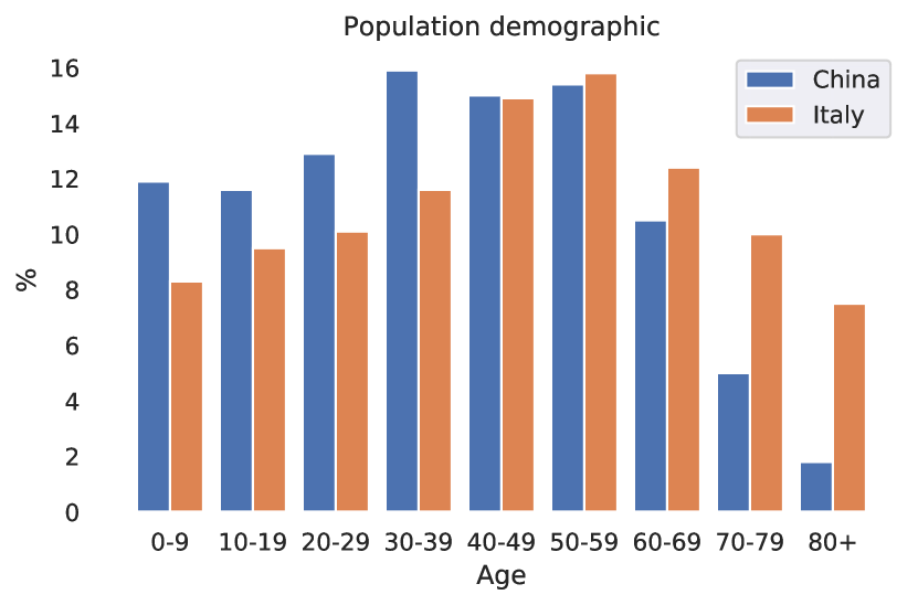
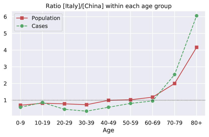
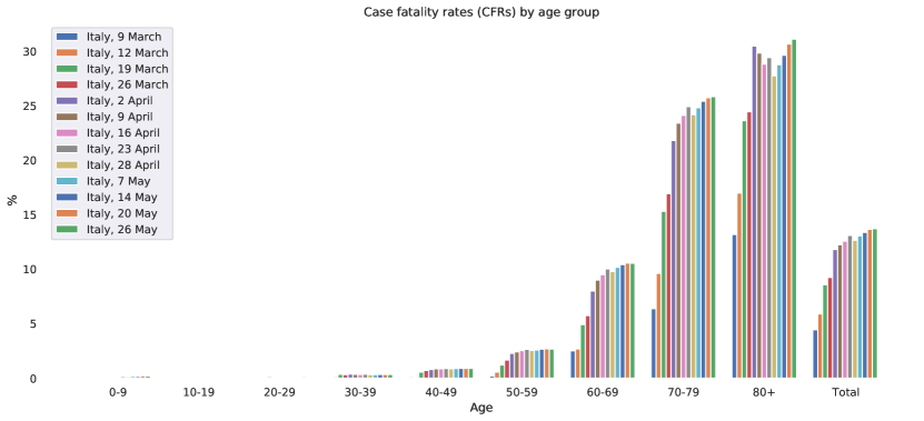
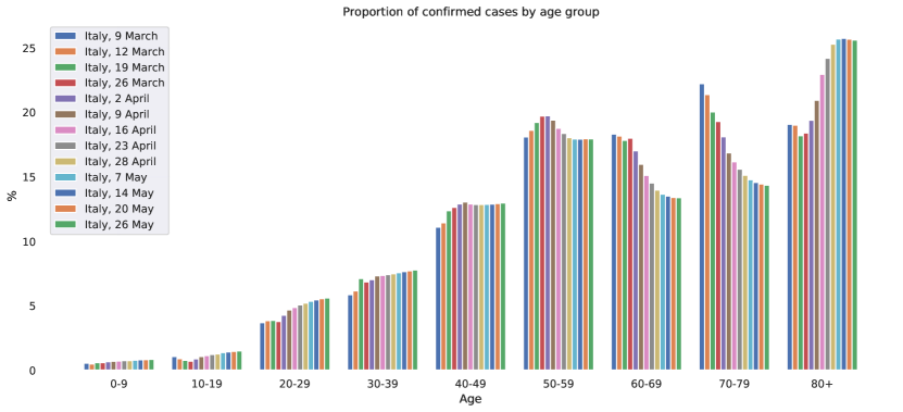
In this Appendix, we provide additional details on the comparison of Italy and China that gives rise to the instance of Simpson’s paradox in section II and that was further investigated with a longitudinal approach in Fig. 3. Tables III, IV, and V show the cfrs, case demographic, and demographic of the general population for the two countries, respectively. The relationship between case demographic and demographic of the general population is further investigated and visualised in Fig. 7. Fig. 8 shows the temporal evolution of age-specific cfrs and case demographic for the longitudinal data from Italy used in Fig. 3.

TABLE III: Exact numbers for the comparison of case fatality rates (cfrs) by age group for Italy and China shown in Fig. 1. Absolute numbers of fatalities/confirmed cases are shown in brackets below. Lower cfrs are highlighted in bold face. Sources: [70] and [29].

Age	0–9	10–19	20–29	30–39	40–49	50–59	60–69	70–79	$\geq$ 80	Total
Italy	0% (0/43)	0% (0/85)	0% (0/296)	0% (0/470)	0.1% (1/891)	0.2% (3/1,453)	2.5% (37/1,471)	6.4% (114/1,785)	13.2% (202/1,532)	4.4% (357/8,026)
China	0%  (0/0)	0.2% (1/549)	0.2% (7/3,619)	0.2% (18/7,600)	0.4% (38/8,571)	1.3% (130/10,008)	3.6% (309/8,583)	8% (312/3,918)	14.8% (208/1,408)	2.3% (1,023/44,672)

TABLE IV: Proportion of confirmed cases from Table III by age group. This corresponds to the case demographics shown in Fig. 1.

Age	0–9	10–19	20–29	30–39	40–49	50–59	60–69	70–79	$\geq$ 80
Italy	0.5%	1.0%	3.5%	5.6%	10.7%	17.4%	17.7%	21.4%	18.4%
China	0.9%	1.2%	8.1%	17.0%	19.2%	22.4%	19.2%	8.8%	3.2%

TABLE V: Age demographic of the general population for Italy and China.

Age	0–9	10–19	20–29	30–39	40–49	50–59	60–69	70–79	$\geq$ 80
Italy	8.3%	9.5%	10.1%	11.6%	14.9%	15.8%	12.4%	10%	7.5%
China	11.9%	11.6%	12.9%	15.9%	15%	15.4%	10.5%	5%	1.8%

(a) Population demographic

(b) Ratios

Figure 7: Visualisation of the data from Tables IV and  V for the demographic comparison of China and Italy. (a) Demographic of the general population in the two countries (c.f. Fig. 1). (b) Ratios (Italy / China) of the proportion of confirmed cases by age group (shown in dashed green) and the proportion of the general population within each age group from Table V (shown in solid red).

Figure 8: Different snapshots from Italy show the temporal evolution of cfrs by age group (top) and case demographic (bottom) over the time period for which different causal effects with China as a control country are shown in Fig. 3.

-E Additional results and figures

-E1 Temporal cfr data for Spain

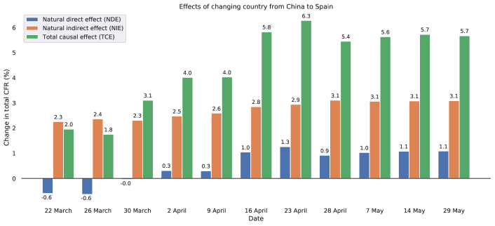
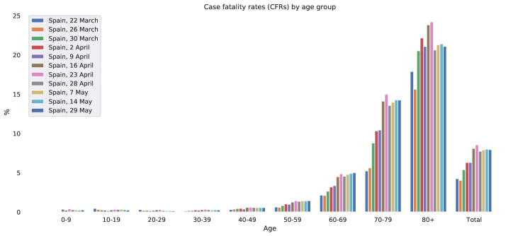
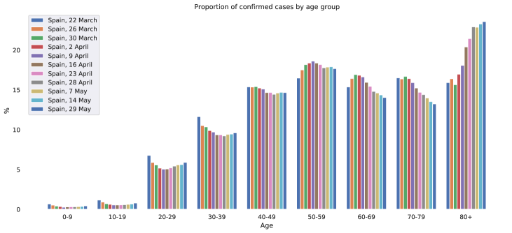
We perform a similar analysis of the temporal evolution of different causal effects of changing country from China to Spain, as done for Italy in section V and Fig. 3. The results are shown in Fig. 9. Recall that the control China remains fixed throughout so that any changes can be attributed to changes in the Spanish data.

Interestingly, a reversal in the sign of the nde can also be observed for Spain, taking place around 30 March. This bears similarity to the reversal of nde observed for Italy. The initial increase in nde is also reflected in the age-specific cfrs shown in the middle of Fig. 9 which are initially increasing for most age groups. Unlike Italy, however, nde and tce do not increase monotonically, but reach a maximum (over the time period considered) around 23 April and subsequently decrease again. The nie also appears less constant than for the case of changing country to Italy shown in Fig. 3, steadily climbing from initially 2.3% to 3.1% at the end of May (ca. 35% increase).

As a remark of caution, we point out that the total number of fatalities reported by the Spanish ministry in age-stratified form is considerably lower than the number of fatalities reported (without separation into age groups) by different sources such as, e.g., [32]. This may have different reasons such as, e.g., latency in their reporting of fatalities in general, or of the exact age group of deceased patients specifically. As a result, cfrs from Spain are lower than other sources suggest, and may thus not be very reliable.

Figure 9: (top) We use different snapshots from Spain to trace tce, nde, and nie of changing country from China to Spain over a time period of  9 weeks, similar to what is shown in Fig. 3 for Italy. We also show the underlying evolution of CFRs by age group (middle) and case demographic (bottom) for the time points considered.

-E2 Comparison of age-specific cfrs and case demographic between different countries

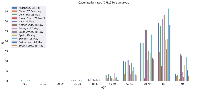
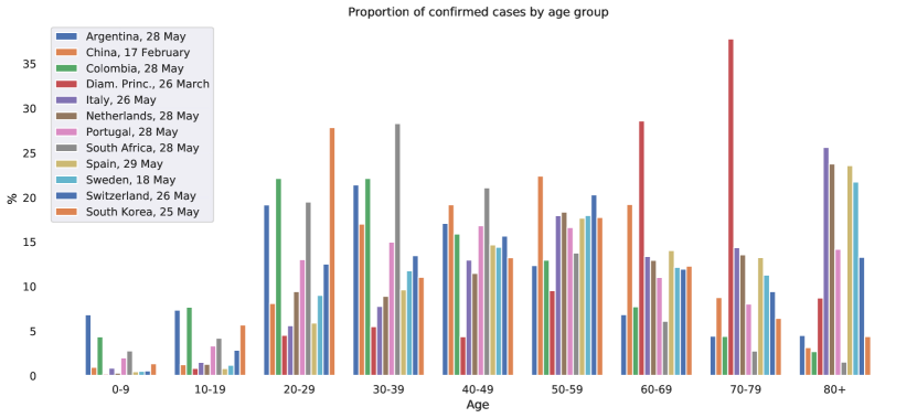
A visual comparison of cfrs by age group and case demographic (similar to that shown in Fig. 1 for only China and Italy) for all different countries in our dataset is shown in Fig. 10.

Figure 10: Comparison of cfrs by age group (top) and case demographic (bottom) for all different countries included in our dataset.

-E3 TCEs between different countries

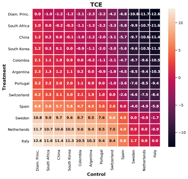
In addition to the pair-wise ndes and nies between the different countries in our dataset, we also show the pair-wise tces for completeness in Fig. 11. Note that—as opposed to nde and nie—the tce is, by definition, symmetric, i.e., $\textsc{tce}_{0\rightarrow 1}=-\textsc{tce}_{1\rightarrow 0}$, as can be seen from Fig. 11.

Figure 11: Total causal effects (tces) for switching from the control country (columns) to the treatment country (rows). Numbers show the change in total cfr in %, i.e., negative numbers indicate that switching to the treatment country’s approach in terms of both cfrs by age group and case demographic would lead to a decrease in total cfr. Countries are ordered by their average treatment effect over the remaining 11 data points as a control.

-F Dataset details

In this Appendix, we provide further details on the datasets of age-stratified case and fatality numbers curated as part of this work. We provide three different datasets:

• A dataset containing the latest age-stratified case and fatality numbers for all different countries considered in our analysis, described in more detail in -F1.

• A dataset containing longitudinal age-stratified case and fatality numbers for Italy, described in more detail in -F2.

• A dataset containing longitudinal age-stratified case and fatality numbers for Spain, described in more detail in -F3.

All datasets are contained in the supplementary material in multiple commonly-used formats (.csv, .xlsx, .json, .pkl) and will be made publicly available upon publication.

-F1 Dataset of latest age-stratified case and fatality numbers for different countries

An overview of the dataset of latest age-stratified case and fatality numbers for different countries in the form of metadata is shown in Table VI.

cfrs and absolute case and fatality numbers in age-stratified form are shown in Table VII.

Case demographics are shown in Table VIII.

TABLE VI: Information on the sources for the data regarding the countries in the case study.

Country	Date of reporting	Confirmed cases	Fatalities	Source
Argentina	28 May	14,675	507	[40]
China	17 February	44,672	1023	[70]
Colombia	28 May	25,366	822	[28]
Diam. Princ.	26 March	619	7	[59]
Italy	26 May	230,760	31676	[30]
Netherlands	28 May	45,947	5903	[57]
Portugal	28 May	31,596	1369	[62]
South Africa	28 May	27,280	577	[26]
South Korea	25 May	11,190	266	[34]
Spain	29 May	258,760	20585	[12]
Sweden	18 May	34,432	4125	[20]
Switzerland	26 May	30,707	1648	[19]

TABLE VII: Exact numbers for the comparison of case fatality rates (cfrs) by age group for all countries discussed in section V. Absolute numbers of fatalities/confirmed cases are shown in brackets below.

Age	0–9	10–19	20–29	30–39	40–49	50–59	60–69	70–79	$\geq$ 80	Total
Argentina	0.0% (0/1,002)	0.1% (1/1,080)	0.0% (1/2,813)	0.3% (9/3,142)	1.0% (24/2,508)	3.0% (54/1,812)	10.0% (101/1,005)	18.9% (123/651)	29.3% (194/662)	3.5% (507/14,675)
China	0.0% (0/416)	0.2% (1/549)	0.2% (7/3,619)	0.2% (18/7,600)	0.4% (38/8,571)	1.3% (130/10,008)	3.6% (309/8,583)	8.0% (312/3,918)	14.8% (208/1,408)	2.3% (1,023/44,672)
Colombia	0.5% (5/1,105)	0.1% (1/1,950)	0.2% (13/5,614)	0.4% (24/5,615)	1.5% (61/4,033)	3.7% (121/3,286)	9.8% (192/1,961)	19.2% (214/1,117)	27.9% (191/685)	3.2% (822/25,366)
Diam. Princ.	0.0% (0/1)	0.0% (0/5)	0.0% (0/28)	0.0% (0/34)	0.0% (0/27)	0.0% (0/59)	0.0% (0/177)	1.3% (3/234)	7.4% (4/54)	1.1% (7/619)
Italy	0.2% (4/1,919)	0.0% (0/3,442)	0.1% (12/12,933)	0.3% (62/17,934)	0.9% (273/29,942)	2.7% (1,109/41,435)	10.6% (3,259/30,880)	25.8% (8,562/33,141)	31.1% (18,395/59,134)	13.7% (31,676/230,760)
Netherlands	0.0% (0/128)	0.2% (1/587)	0.1% (3/4,336)	0.2% (10/4,093)	0.5% (28/5,269)	1.7% (142/8,437)	8.1% (484/5,949)	25.6% (1,596/6,229)	33.3% (3,639/10,919)	12.8% (5,903/45,947)
Portugal	0.0% (0/626)	0.0% (0/1,052)	0.0% (1/4,114)	0.0% (1/4,736)	0.3% (15/5,315)	0.8% (42/5,253)	3.5% (122/3,484)	10.6% (269/2,537)	20.5% (919/4,479)	4.3% (1,369/31,596)
South Africa	0.3% (2/755)	0.1% (1/1,147)	0.1% (4/5,319)	0.4% (33/7,720)	1.1% (61/5,754)	3.8% (144/3,753)	9.2% (153/1,663)	15.0% (113/754)	15.9% (66/415)	2.1% (577/27,280)
South Korea	0.0% (0/149)	0.0% (0/636)	0.0% (0/3,117)	0.2% (2/1,235)	0.2% (3/1,481)	0.8% (15/1,987)	2.8% (39/1,375)	10.8% (78/719)	26.3% (129/491)	2.4% (266/11,190)
Spain	0.3% (3/1,123)	0.2% (5/2,068)	0.2% (24/15272)	0.3% (65/24,902)	0.6% (218/37,970)	1.4% (663/45750)	5.0% (1,825/36,355)	14.3% (4,896/34,294)	21.1% (12,886/61,026)	8.0% (20,585/258,760)
Sweden	0.6% (1/168)	0.0% (0/401)	0.3% (8/3,104)	0.3% (12/4,051)	0.8% (39/4,962)	2.1% (129/6,190)	7.0% (294/4,186)	23.4% (909/3,888)	36.5% (2,733/7,482)	12.0% (4,125/34,432)
Switzerland	0.0% (0/162)	0.0% (0/877)	0.0% (0/3,844)	0.1% (5/4,136)	0.1% (4/4,809)	0.6% (37/6,232)	3.3% (121/3,671)	11.6% (335/2,896)	28.1% (1,146/4,080)	5.4% (1,648/30,707)

TABLE VIII: Proportion of confirmed cases by age group for all of the countries considered in section V.

Age	0–9	10–19	20–29	30–39	40–49	50–59	60–69	70–79	$\geq$ 80
Argentina	6.8%	7.4%	19.2%	21.4%	17.1%	12.3%	6.8%	4.4%	4.6%
China	0.9%	1.2%	8.1%	17.0%	19.2%	22.4%	19.2%	8.8%	3.2%
Colombia	4.4%	7.7%	22.1%	22.1%	15.9%	13.0%	7.7%	4.4%	2.7%
Diam. Princ.	0.2%	0.8%	4.5%	5.5%	4.4%	9.5%	28.6%	37.8%	8.7%
Italy	0.8%	1.5%	5.6%	7.8%	13.0%	18.0%	13.4%	14.4%	25.5%
Netherlands	0.3%	1.3%	9.4%	8.9%	11.5%	18.4%	12.9%	13.6%	23.7%
Portugal	2.0%	3.3%	13.0%	15.0%	16.8%	16.6%	11.0%	8.0%	14.3%
South Africa	2.8%	4.2%	19.5%	28.3%	21.1%	13.8%	6.1%	2.8%	1.4%
South Korea	1.3%	5.7%	27.9%	11.0%	13.2%	17.8%	12.3%	6.4%	4.4%
Spain	0.4%	0.8%	5.9%	9.6%	14.7%	17.7%	14.0%	13.3%	23.6%
Sweden	0.5%	1.2%	9.0%	11.8%	14.4%	18.0%	12.2%	11.3%	21.7%
Switzerland	0.5%	2.9%	12.5%	13.5%	15.7%	20.3%	12.0%	9.4%	13.2%

-F2 Dataset of longitudinal age-stratified case and fatality numbers for Italy

An overview of the dataset of longitudinal age-stratified case and fatality numbers for Italy, in the form of metadata, is shown in Table IX. The source for all different time points is the same as that shown in Table VI for Italy, queried at the corresponding dates shown in Table IX. cfrs and absolute case and fatality numbers in age-stratified form are shown in Table X. Case demographics are shown in Table XI.

TABLE IX: Metadata for the longitudinal data from Italy.

Date of reporting	Confirmed cases	Fatalities
9 March	8,026	357
12 March	13,317	785
19 March	35,529	3,047
23 March	57,695	5,018
26 March	73,534	6,801
2 April	106,231	12,548
9 April	135,968	16,653
16 April	159,003	19,994
23 April	177,025	23,118
28 April	199,389	25,215
7 May	214,047	27,955
14 May	222,022	29,691
20 May	227,153	31,017
26 May	230,760	31,676

TABLE X: Age-specific cfrs for the longitudinal data for Italy.

Age	0–9	10–19	20–29	30–39	40–49	50–59	60–69	70–79	$\geq$ 80	Total
9 March	0.0% (0/43)	0.0% (0/85)	0.0% (0/296)	0.0% (0/470)	0.1% (1/891)	0.2% (3/1453)	2.5% (37/1471)	6.4% (114/1785)	13.2% (202/1532)	4.4% (357/8026)
12 March	0.0% (0/63)	0.0% (0/118)	0.0% (0/511)	0.1% (1/819)	0.1% (1/1523)	0.6% (14/2480)	2.7% (65/2421)	9.6% (274/2849)	17.0% (430/2533)	5.9% (785/13317)
19 March	0.0% (0/205)	0.0% (0/270)	0.0% (0/1374)	0.4% (9/2525)	0.6% (25/4396)	1.2% (83/6834)	4.9% (312/6337)	15.3% (1090/7121)	23.6% (1528/6467)	8.6% (3047/35529)
23 March	0.0% (0/318)	0.0% (0/386)	0.0% (0/2192)	0.3% (12/3995)	0.6% (41/7267)	1.5% (168/11280)	5.2% (541/10423)	15.6% (1768/11320)	23.7% (2488/10514)	8.7% (5018/57695)
26 March	0.0% (0/428)	0.0% (0/512)	0.0% (0/2778)	0.3% (17/5033)	0.7% (67/9295)	1.7% (243/14508)	5.7% (761/13243)	16.9% (2403/14198)	24.4% (3310/13539)	9.2% (6801/73534)
2 April	0.0% (0/693)	0.0% (0/931)	0.1% (6/4530)	0.4% (29/7466)	0.8% (110/13701)	2.3% (479/20975)	8.0% (1448/18089)	21.8% (4196/19238)	30.5% (6280/20608)	11.8% (12548/106231)
9 April	0.1% (1/938)	0.0% (0/1432)	0.1% (7/6360)	0.4% (36/9956)	0.9% (153/17745)	2.4% (638/26391)	9.0% (1957/21734)	23.4% (5366/22934)	29.8% (8495/28478)	12.2% (16653/135968)
16 April	0.1% (1/1123)	0.0% (0/1804)	0.1% (7/7737)	0.3% (40/11686)	0.9% (178/20519)	2.5% (756/29858)	9.5% (2284/24040)	24.1% (6203/25717)	28.8% (10525/36519)	12.6% (19994/159003)
23 April	0.2% (2/1304)	0.0% (0/2146)	0.1% (7/8963)	0.4% (48/13137)	0.9% (203/22767)	2.6% (861/32524)	10.0% (2576/25707)	24.9% (6882/27615)	29.4% (12609/42862)	13.1% (23188/177025)
28 April	0.1% (2/1478)	0.0% (0/2511)	0.1% (8/10377)	0.3% (49/14907)	0.9% (224/25644)	2.6% (918/35986)	9.8% (2727/27880)	24.2% (7291/30158)	27.7% (13996/50448)	12.6% (25215/199389)
7 May	0.2% (3/1642)	0.0% (0/2908)	0.1% (9/11457)	0.3% (54/16189)	0.9% (246/27553)	2.6% (993/38399)	10.2% (2976/29252)	24.8% (7849/31627)	28.8% (15825/55020)	13.1% (27955/214047)
14 May	0.2% (3/1774)	0.0% (0/3148)	0.1% (12/12115)	0.3% (59/16981)	0.9% (258/28627)	2.7% (1063/39822)	10.4% (3127/30010)	25.4% (8221/32353)	29.6% (16948/57192)	13.4% (29691/222022)
20 May	0.2% (4/1851)	0.0% (0/3312)	0.1% (14/12599)	0.3% (61/17528)	0.9% (268/29390)	2.7% (1101/40803)	10.6% (3219/30466)	25.7% (8447/32824)	30.7% (17903/58380)	13.7% (31017/227153)
26 May	0.2% (4/1919)	0.0% (0/3442)	0.1% (12/12933)	0.3% (62/17934)	0.9% (273/29942)	2.7% (1109/41435)	10.6% (3259/30880)	25.8% (8562/33141)	31.1% (18395/59134)	13.7% (31676/230760)

TABLE XI: Proportion of confirmed cases by age group for longitudinal data for Italy.

Age	0–9	10–19	20–29	30–39	40–49	50–59	60–69	70–79	$\geq$ 80
9 March	0.5%	1.1%	3.7%	5.9%	11.1%	18.1%	18.3%	22.2%	19.1%
12 March	0.5%	0.9%	3.8%	6.2%	11.4%	18.6%	18.2%	21.4%	19.0%
19 March	0.6%	0.8%	3.9%	7.1%	12.4%	19.2%	17.8%	20.0%	18.2%
23 March	0.6%	0.7%	3.8%	6.9%	12.6%	19.6%	18.1%	19.6%	18.1%
26 March	0.6%	0.7%	3.8%	6.8%	12.6%	19.7%	18.0%	19.3%	18.5%
2 April	0.7%	0.9%	4.3%	7.0%	12.9%	19.7%	17.0%	18.1%	19.4%
9 April	0.7%	1.1%	4.7%	7.3%	13.1%	19.4%	16.0%	16.9%	20.8%
16 April	0.7%	1.1%	4.9%	7.3%	12.9%	18.8%	15.1%	16.2%	23.0%
23 April	0.7%	1.2%	5.1%	7.4%	12.9%	18.4%	14.5%	15.6%	24.2%
28 April	0.7%	1.3%	5.2%	7.5%	12.9%	18.0%	14.0%	15.1%	25.3%
7 May	0.8%	1.4%	5.4%	7.6%	12.9%	17.9%	13.7%	14.7%	25.6%
14 May	0.8%	1.4%	5.5%	7.6%	12.9%	17.9%	13.5%	14.6%	25.8%
20 May	0.8%	1.5%	5.5%	7.7%	12.9%	18.0%	13.4%	14.5%	25.7%
26 May	0.8%	1.5%	5.6%	7.8%	13.0%	18.0%	13.4%	14.4%	25.5%

-F3 Dataset of longitudinal age-stratified case and fatality numbers for Spain

An overview of the dataset of longitudinal age-stratified case and fatality numbers for Spain, in the form of metadata, is shown in Table XII. The source for all different time points is the same as that shown in Table VI for Spain, queried at the corresponding dates shown in Table XII.

cfrs and absolute case and fatality numbers in age-stratified form are shown in Table XIII.

Case demographics are shown in Table XIV.

TABLE XII: Metadata for the longitudinal data from Spain.

Date of reporting	Confirmed cases	Fatalities
22 March	18,959	805
26 March	32,816	1,326
30 March	51,626	2,784
2 April	69,177	4,361
9 April	106,447	6,729
16 April	133,082	10,793
23 April	152,687	13,078
28 April	204,866	15,853
7 May	220,444	17,460
14 May	239,095	19,115
29 May	258,760	20,585

TABLE XIII: Longitudinal age-stratified data for Spain.

Age	0–9	10–19	20–29	30–39	40–49	50–59	60–69	70–79	$\geq$ 80	Total
22 March	0.0% (0/129)	0.5% (1/221)	0.3% (4/1285)	0.1% (3/2208)	0.3% (9/2919)	0.6% (20/3129)	2.2% (63/2916)	5.2% (164/3132)	17.9% (541/3020)	4.2% (805/18959)
26 March	0.0% (0/175)	0.3% (1/302)	0.2% (4/1932)	0.2% (7/3454)	0.4% (19/5045)	0.6% (35/5749)	2.1% (114/5397)	5.6% (303/5377)	15.7% (843/5385)	4.0% (1326/32816)
30 March	0.0% (0/212)	0.3% (1/368)	0.2% (6/2883)	0.2% (10/5351)	0.5% (36/7965)	0.8% (78/9390)	2.7% (232/8744)	8.8% (759/8625)	20.5% (1662/8088)	5.4% (2784/51626)
2 April	0.0% (0/250)	0.2% (1/434)	0.2% (6/3590)	0.3% (18/6853)	0.5% (49/10551)	1.0% (131/12722)	3.2% (373/11657)	10.3% (1176/11368)	22.2% (2607/11752)	6.3% (4361/69177)
9 April	0.4% (1/285)	0.2% (1/588)	0.2% (11/5381)	0.2% (24/10341)	0.4% (61/16088)	1.0% (197/19836)	3.4% (597/17713)	10.5% (1773/16957)	21.1% (4064/19258)	6.3% (6729/106447)
16 April	0.2% (1/423)	0.3% (2/734)	0.3% (19/6763)	0.3% (37/12466)	0.6% (116/19536)	1.3% (312/24471)	4.5% (958/21249)	14.1% (2868/20287)	23.9% (6480/27153)	8.1% (10793/133082)
23 April	0.4% (2/502)	0.3% (3/869)	0.3% (25/7962)	0.3% (50/14304)	0.6% (138/22430)	1.4% (400/27795)	4.9% (1149/23595)	15.0% (3374/22470)	24.2% (7937/32760)	8.6% (13078/152687)
28 April	0.3% (2/660)	0.3% (4/1206)	0.2% (22/11138)	0.3% (55/18924)	0.6% (172/29629)	1.4% (497/36423)	4.6% (1387/30361)	13.6% (4012/29550)	20.7% (9702/46975)	7.7% (15853/204866)
7 May	0.3% (2/765)	0.4% (5/1398)	0.2% (21/12321)	0.3% (57/20759)	0.6% (185/32239)	1.4% (569/39418)	4.8% (1541/32226)	14.0% (4320/30861)	21.3% (10760/50457)	7.9% (17460/220444)
14 May	0.2% (2/871)	0.3% (5/1619)	0.2% (23/13439)	0.3% (62/22643)	0.6% (201/35175)	1.4% (610/42874)	4.9% (1693/34380)	14.3% (4628/32395)	21.4% (11931/55699)	8.0% (19155/239095)
29 May	0.3% (3/1123)	0.2% (5/2068)	0.2% (24/15272)	0.3% (65/24902)	0.6% (218/37970)	1.4% (663/45750)	5.0% (1825/36355)	14.3% (4896/34294)	21.1% (12886/61026)	8.0% (20585/258760)

TABLE XIV: Proportion of confirmed cases by age group for the longitudinal data from Spain.

Age	0–9	10–19	20–29	30–39	40–49	50–59	60–69	70–79	$\geq$ 80
22 March	0.5%	2.9%	12.5%	13.5%	15.7%	20.3%	12.0%	9.4%	13.2%
26 March	0.5%	0.9%	5.9%	10.5%	15.4%	17.5%	16.4%	16.4%	16.5%
30 March	0.4%	0.7%	5.6%	10.4%	15.4%	18.2%	16.9%	16.7%	15.7%
2 April	0.4%	0.6%	5.2%	9.9%	15.3%	18.4%	16.9%	16.4%	16.9%
9 April	0.3%	0.6%	5.1%	9.7%	15.1%	18.6%	16.6%	15.9%	18.1%
16 April	0.3%	0.6%	5.1%	9.4%	14.7%	18.4%	16.0%	15.2%	20.3%
23 April	0.3%	0.6%	5.2%	9.4%	14.7%	18.2%	15.5%	14.7%	21.4%
28 April	0.3%	0.6%	5.4%	9.2%	14.5%	17.8%	14.8%	14.4%	23.0%
7 May	0.3%	0.6%	5.6%	9.4%	14.6%	17.9%	14.6%	14.0%	23.0%
14 May	0.4%	0.7%	5.6%	9.5%	14.7%	17.9%	14.4%	13.5%	23.3%
29 May	0.4%	0.8%	5.9%	9.6%	14.7%	17.7%	14.0%	13.3%	23.6%

References

- Alsdurf et al. [2020] Hannah Alsdurf, Edmond Belliveau, Yoshua Bengio, Tristan Deleu, Prateek Gupta, Daphne Ippolito, Richard Janda, Max Jarvie, Tyler Kolody, Sekoul Krastev, et al. COVI white paper. arXiv e-prints, pages arXiv–2005, 2020.
- Armocida et al. [2020] Benedetta Armocida, Beatrice Formenti, Silvia Ussai, Francesca Palestra, and Eduardo Missoni. The Italian health system and the COVID-19 challenge. The Lancet Public Health, 2020.
- Bareinboim and Pearl [2016] Elias Bareinboim and Judea Pearl. Causal inference and the data-fusion problem. Proceedings of the National Academy of Sciences, 113(27):7345–7352, 2016.
- Bareinboim and Tian [2015] Elias Bareinboim and Jin Tian. Recovering causal effects from selection bias. In Twenty-Ninth AAAI Conference on Artificial Intelligence, 2015.
- Bareinboim et al. [2015] Elias Bareinboim, Andrew Forney, and Judea Pearl. Bandits with unobserved confounders: A causal approach. Advances in Neural Information Processing Systems, 28:1342–1350, 2015.
- Barstugan et al. [2020] Mucahid Barstugan, Umut Ozkaya, and Saban Ozturk. Coronavirus (Covid-19) classification using CT images by machine learning methods. arXiv preprint arXiv:2003.09424, 2020.
- Barthe et al. [2021] Gilles Barthe, Roberta De Viti, Peter Druschel, Deepak Garg, Manuel Gomez Rodriguez, Pierfrancesco Ingo, Heiner Kremer, Matthew Lentz, Lars Lorch, Aastha Mehta, et al. Listening to bluetooth beacons for epidemic risk mitigation. medRxiv, 2021.
- Baud et al. [2020] David Baud, Xiaolong Qi, Karin Nielsen-Saines, Didier Musso, Léo Pomar, and Guillaume Favre. Real estimates of mortality following COVID-19 infection. The Lancet Infectious Diseases, 2020.
- Bayer and Kuhn [2020] Christian Bayer and Moritz Kuhn. Intergenerational ties and case fatality rates: A cross-country analysis. Technical report, Institute of Labor Economics (IZA), 2020.
- Besserve et al. [2020] Michel Besserve, Simon Buchholz, and Bernhard Schölkopf. Assaying large-scale testing models to interpret Covid-19 case numbers. a cross-country study. arXiv preprint arXiv:2012.01912, 2020.
- Bickel et al. [1975] Peter J Bickel, Eugene A Hammel, and J William O’Connell. Sex bias in graduate admissions: Data from Berkeley. Science, 187(4175):398–404, 1975.
- Centro de Coordinación de Alertas y Emergencias Sanitarias; , Ministerio de Sanidad, Consumo y Bienestar Social; (MISAN, Ministry of Health, Consumer Affairs and Social Welfare)(2020) [CCAES] Centro de Coordinación de Alertas y Emergencias Sanitarias; (CCAES), Ministerio de Sanidad, Consumo y Bienestar Social; (MISAN, Ministry of Health, Consumer Affairs and Social Welfare). 29 May report. https://www.mscbs.gob.es/profesionales/saludPublica/ccayes/alertasActual/nCov-China/documentos/Actualizacion_120_COVID-19.pdf, 2020.
- Cereda et al. [2020] Diletta Cereda, Marcello Tirani, Francesca Rovida, Vittorio Demicheli, Marco Ajelli, Piero Poletti, Frédéric Trentini, Giorgio Guzzetta, Valentina Marziano, Angelica Barone, et al. The early phase of the COVID-19 outbreak in lombardy, italy, 2020.
- Chernozhukov et al. [2021] Victor Chernozhukov, Hiroyuki Kasahara, and Paul Schrimpf. Causal impact of masks, policies, behavior on early Covid-19 pandemic in the US. Journal of Econometrics, 220(1):23–62, 2021.
- Chiappa [2019] Silvia Chiappa. Path-specific counterfactual fairness. In Proceedings of the AAAI Conference on Artificial Intelligence, volume 33, pages 7801–7808, 2019.
- Cohen and Nagel [1936] Morris R Cohen and Ernest Nagel. Introduction to logic and scientific method. Allied Publishers Private Limited, New Delhi, 1936.
- Correa et al. [2019] Juan Correa, Jin Tian, and Elias Bareinboim. Adjustment criteria for generalizing experimental findings. In International Conference on Machine Learning, pages 1361–1369, 2019.
- Elaziz et al. [2020] Mohamed Abd Elaziz, Khalid M Hosny, Ahmad Salah, Mohamed M Darwish, Songfeng Lu, and Ahmed T Sahlol. New machine learning method for image-based diagnosis of COVID-19. Plos one, 15(6):e0235187, 2020.
- Federal Office of Public Health Switzerland [2020] Federal Office of Public Health Switzerland. 26 May report. https://www.bag.admin.ch/bag/en/home/krankheiten/ausbrueche-epidemien-pandemien/aktuelle-ausbrueche-epidemien/novel-cov/situation-schweiz-und-international.html#-1199962081, 2020.
- Folkhalsomyndigheten (2020) [Public Health Agency of Sweden] Folkhalsomyndigheten (Public Health Agency of Sweden). 18 May report. https://en.wikipedia.org/wiki/COVID-19_pandemic_in_Sweden#cite_note-306, 2020. Accessed 29 May.
- Forney et al. [2017] Andrew Forney, Judea Pearl, and Elias Bareinboim. Counterfactual data-fusion for online reinforcement learners. In International Conference on Machine Learning, pages 1156–1164. PMLR, 2017.
- Griffith et al. [2020] Gareth J Griffith, Tim T Morris, Matthew J Tudball, Annie Herbert, Giulia Mancano, Lindsey Pike, Gemma C Sharp, Jonathan Sterne, Tom M Palmer, George Davey Smith, et al. Collider bias undermines our understanding of COVID-19 disease risk and severity. Nature communications, 11(1):1–12, 2020.
- Harmer et al. [1999] Greg P Harmer, Derek Abbott, et al. Parrondo’s paradox. Statistical Science, 14(2):206–213, 1999.
- Harmer and Abbott [2002] Gregory P Harmer and Derek Abbott. A review of Parrondo’s paradox. Fluctuation and Noise Letters, 2(02):R71–R107, 2002.
- Health [2021] The Lancet Digital Health. Artificial intelligence for COVID-19: saviour or saboteur? The Lancet. Digital Health, 3(1):e1, 2021.
- Health Department republic of South Africa [2020] Health Department republic of South Africa. 28 May report. https://sacoronavirus.co.za/2020/05/29/update-on-covid-19-28th-may-2020/, 2020. Accessed 29 May.
- Hernán et al. [2011] Miguel A Hernán, David Clayton, and Niels Keiding. The Simpson’s paradox unraveled. International journal of epidemiology, 40(3):780–785, 2011.
- Instituto Nacional de Salud [2020] Instituto Nacional de Salud. 28 May report. https://www.ins.gov.co/Noticias/Paginas/Coronavirus.aspx, 2020.
- Istituto Superiore di Sanità [2020] Istituto Superiore di Sanità. Epidemia COVID-19: Aggiornamento nazionale, 09 Marzo 2020 – ore 16:00. https://www.epicentro.iss.it/coronavirus/bollettino/Bollettino-sorveglianza-integrata-COVID-19_09-marzo-2020.pdf, 2020.
- Istituto Superiore di Sanità (2020) [ISS, Italian National Institute of Health] Istituto Superiore di Sanità (ISS, Italian National Institute of Health). 26 May report. https://www.epicentro.iss.it/coronavirus/bollettino/Bollettino-sorveglianza-integrata-COVID-19_26-maggio-2020.pdf, 2020.
- Jain et al. [1999] Anil K Jain, M Narasimha Murty, and Patrick J Flynn. Data clustering: a review. ACM computing surveys (CSUR), 31(3):264–323, 1999.
- Johns Hopkins University [Retrieved 28 September 2020] Johns Hopkins University. COVID-19 dashboard by the center for systems science and engineering (csse). https://coronavirus.jhu.edu/map.html, Retrieved 28 September 2020.
- Kilbertus et al. [2017] Niki Kilbertus, Mateo Rojas-Carulla, Giambattista Parascandolo, Moritz Hardt, Dominik Janzing, and Bernhard Schölkopf. Avoiding discrimination through causal reasoning. In Proceedings of the 31st International Conference on Neural Information Processing Systems, pages 656–666, 2017.
- Korea Centers for Disease Control and Prevention [2020] Korea Centers for Disease Control and Prevention. 25 May report. https://www.cdc.go.kr/board/board.es?mid=a20501000000&bid=0015&list_no=367317&act=view, 2020.
- Korolev [2020] Ivan Korolev. What does the case fatality ratio really measure? Available at SSRN 3572891, 2020.
- Kusner et al. [2017] MJ Kusner, J Loftus, Christopher Russell, and R Silva. Counterfactual fairness. Advances in Neural Information Processing Systems 30, 30, 2017.
- Lalmuanawma et al. [2020] Samuel Lalmuanawma, Jamal Hussain, and Lalrinfela Chhakchhuak. Applications of machine learning and artificial intelligence for Covid-19 (SARS-CoV-2) pandemic: A review. Chaos, Solitons & Fractals, page 110059, 2020.
- Latif et al. [2020] Siddique Latif, Muhammad Usman, Sanaullah Manzoor, Waleed Iqbal, Junaid Qadir, Gareth Tyson, Ignacio Castro, Adeel Razi, Maged N Kamel Boulos, Adrian Weller, et al. Leveraging data science to combat Covid-19: A comprehensive review. IEEE Transactions on Artificial Intelligence, 2020.
- Mackenzie [2020] Dana Mackenzie. Race, COVID mortality, and Simpson’s paradox. http://causality.cs.ucla.edu/blog/index.php/2020/07/06/race-covid-mortality-and-simpsons-paradox-by-dana-mackenzie/ (Retrieved July 6), 2020.
- Ministry of Health of Argentina [2020] Ministry of Health of Argentina. 28 May report. https://www.argentina.gob.ar/salud/coronavirus-COVID-19/sala-situacion, 2020. Accessed 29 May.
- Mossong et al. [2008] Joël Mossong, Niel Hens, Mark Jit, Philippe Beutels, Kari Auranen, Rafael Mikolajczyk, Marco Massari, Stefania Salmaso, Gianpaolo Scalia Tomba, Jacco Wallinga, et al. Social contacts and mixing patterns relevant to the spread of infectious diseases. PLoS Medicine, 5(3), 2008.
- Neufeld [1995] Eric Neufeld. Simpson’s paradox in artificial intelligence and in real life. Computational intelligence, 11(1):1–10, 1995.
- Novick [1983] Melvin R. Novick. The centrality of lord’s paradox and exchangeability for all statistical inference. Principals of modern psychological measurement: A festschrift for Frederic M. Lord, page 41, 1983.
- Ong et al. [2020] Edison Ong, Mei U Wong, Anthony Huffman, and Yongqun He. COVID-19 coronavirus vaccine design using reverse vaccinology and machine learning. Frontiers in immunology, 11:1581, 2020.
- Pearl [2001] Judea Pearl. Direct and indirect effects. In Proceedings of the Seventeenth conference on Uncertainty in artificial intelligence, pages 411–420, 2001.
- Pearl [2009] Judea Pearl. Causality. Cambridge University Press, 2009.
- Pearl [2013] Judea Pearl. Understanding Simpson’s paradox. Available at SSRN 2343788, 2013.
- Pearl [2014] Judea Pearl. Comment: understanding simpson’s paradox. The American Statistician, 68(1):8–13, 2014.
- Pearl and Mackenzie [2018] Judea Pearl and Dana Mackenzie. The book of why: the new science of cause and effect. Basic Books, 2018.
- Pearl et al. [2014] Judea Pearl, Elias Bareinboim, et al. External validity: From do-calculus to transportability across populations. Statistical Science, 29(4):579–595, 2014.
- Perez-Saez et al. [2020] Javier Perez-Saez, Stephen A Lauer, Laurent Kaiser, Simon Regard, Elisabeth Delaporte, Idris Guessous, Silvia Stringhini, Andrew S Azman, Serocov-POP Study Group, et al. Serology-informed estimates of SARS-COV-2 infection fatality risk in geneva, switzerland. medRxiv, 2020.
- Peters et al. [2017] Jonas Peters, Dominik Janzing, and Bernhard Schölkopf. Elements of causal inference: foundations and learning algorithms. MIT Press, 2017.
- Poletti et al. [2020] Piero Poletti, Marcello Tirani, Danilo Cereda, Filippo Trentini, Giorgio Guzzetta, Valentina Marziano, Sabrina Buoro, Simona Riboli, Lucia Crottogini, Raffaella Piccarreta, et al. Age-specific SARS-CoV-2 infection fatality ratio and associated risk factors, Italy, February to April 2020. Eurosurveillance, 25(31):2001383, 2020.
- Prem et al. [2020] Kiesha Prem, Yang Liu, Timothy W Russell, Adam J Kucharski, Rosalind M Eggo, Nicholas Davies, Stefan Flasche, Samuel Clifford, Carl AB Pearson, James D Munday, et al. The effect of control strategies to reduce social mixing on outcomes of the COVID-19 epidemic in wuhan, china: a modelling study. The Lancet Public Health, 2020.
- Rajgor et al. [2020] Dimple D Rajgor, Meng Har Lee, Sophia Archuleta, Natasha Bagdasarian, and Swee Chye Quek. The many estimates of the COVID-19 case fatality rate. The Lancet Infectious Diseases, 2020.
- Reichenbach [1956] Hans Reichenbach. The Direction of Time. University of California Press, Berkeley, CA, 1956.
- Rijksinstituut voor Volksgezondheid en Milieu [2020] Rijksinstituut voor Volksgezondheid en Milieu. 28 May report. https://www.rivm.nl/documenten/epidemiologische-situatie-covid-19-in-nederland-28-mei-2020, 2020.
- Rinaldi and Paradisi [2020] Gianluca Rinaldi and Matteo Paradisi. An empirical estimate of the infection fatality rate of COVID-19 from the first italian outbreak. medRxiv, 2020.
- Russell et al. [2020] Timothy W Russell, Joel Hellewell, Christopher I Jarvis, Kevin Van Zandvoort, Sam Abbott, Ruwan Ratnayake, Stefan Flasche, Rosalind M Eggo, W John Edmunds, Adam J Kucharski, et al. Estimating the infection and case fatality ratio for coronavirus disease (COVID-19) using age-adjusted data from the outbreak on the Diamond Princess cruise ship, February 2020. Eurosurveillance, 25(12):2000256, 2020.
- Schölkopf et al. [2012] B Schölkopf, D Janzing, J Peters, E Sgouritsa, K Zhang, and J Mooij. On causal and anticausal learning. In 29th International Conference on Machine Learning (ICML 2012), pages 1255–1262. International Machine Learning Society, 2012.
- Schwab et al. [2021] Patrick Schwab, Arash Mehrjou, Sonali Parbhoo, Leo Anthony Celi, Jürgen Hetzel, Markus Hofer, Bernhard Schölkopf, and Stefan Bauer. Real-time prediction of COVID-19 related mortality using electronic health records. Nature Communications, 12(1):1–16, 2021.
- Servico Nacional de Saude Republica Portuguesa [2020] Servico Nacional de Saude Republica Portuguesa. 28 May report. https://covid19.min-saude.pt/wp-content/uploads/2020/05/87_DGS_boletim_20200528.pdf, 2020.
- Simpson [1951] Edward H Simpson. The interpretation of interaction in contingency tables. Journal of the Royal Statistical Society: Series B (Methodological), 13(2):238–241, 1951.
- Soltan et al. [2020] Andrew AS Soltan, Samaneh Kouchaki, Tingting Zhu, Dani Kiyasseh, Thomas Taylor, Zaamin B Hussain, Tim Peto, Andrew J Brent, David W Eyre, and David A Clifton. Rapid triage for COVID-19 using routine clinical data for patients attending hospital: development and prospective validation of an artificial intelligence screening test. The Lancet Digital Health, 2020.
- van der Schaar et al. [2021] Mihaela van der Schaar, Ahmed M Alaa, Andres Floto, Alexander Gimson, Stefan Scholtes, Angela Wood, Eoin McKinney, Daniel Jarrett, Pietro Lio, and Ari Ercole. How artificial intelligence and machine learning can help healthcare systems respond to COVID-19. Machine Learning, 110(1):1–14, 2021.
- Verity et al. [2020] Robert Verity, Lucy C Okell, Ilaria Dorigatti, Peter Winskill, Charles Whittaker, Natsuko Imai, Gina Cuomo-Dannenburg, Hayley Thompson, Patrick GT Walker, Han Fu, et al. Estimates of the severity of coronavirus disease 2019: a model-based analysis. The Lancet infectious diseases, 2020.
- von Kügelgen et al. [14 May 2020] Julius von Kügelgen, Luigi Gresele, and Bernhard Schölkopf. Simpson’s paradox in Covid-19 case fatality rates: a mediation analysis of age-related causal effects. arXiv preprint arXiv:2005.07180v1, 14 May 2020.
- WHO [2020] WHO. Statement on the second meeting of the International Health Regulations (2005) Emergency Committee regarding the outbreak of novel coronavirus (2019-nCoV), 2020.
- Wu et al. [2019] Yongkai Wu, Lu Zhang, Xintao Wu, and Hanghang Tong. PC-fairness: A unified framework for measuring causality-based fairness. In Advances in Neural Information Processing Systems 32: Annual Conference on Neural Information Processing Systems 2019, NeurIPS 2019, 2019.
- Wu and McGoogan [2020] Zunyou Wu and Jennifer M McGoogan. Characteristics of and important lessons from the coronavirus disease 2019 (COVID-19) outbreak in China: summary of a report of 72 314 cases from the Chinese Center for Disease Control and Prevention. Jama, 2020.
- Wynants et al. [2020] Laure Wynants, Ben Van Calster, Gary S Collins, Richard D Riley, Georg Heinze, Ewoud Schuit, Marc MJ Bonten, Darren L Dahly, Johanna AA Damen, Thomas PA Debray, et al. Prediction models for diagnosis and prognosis of Covid-19: systematic review and critical appraisal. bmj, 369, 2020.
- Xu et al. [2018] Chenguang Xu, Sarah Brown, and Christan Grant. Detecting simpson’s paradox. In Florida Artificial Intelligence Research Society Conference, 2018.
- Xu and Wunsch [2008] Rui Xu and Don Wunsch. Clustering, volume 10. John Wiley & Sons, 2008.
- Zhang et al. [2020] Juanjuan Zhang, Maria Litvinova, Yuxia Liang, Yan Wang, Wei Wang, Shanlu Zhao, Qianhui Wu, Stefano Merler, Cécile Viboud, Alessandro Vespignani, et al. Changes in contact patterns shape the dynamics of the COVID-19 outbreak in China. Science, 2020.
- Zhang and Bareinboim [2018] Junzhe Zhang and Elias Bareinboim. Fairness in decision-making—the causal explanation formula. In Proceedings of the AAAI Conference on Artificial Intelligence, volume 32, 2018.