Supplementary Material – OctSqueeze: Octree-Structured Entropy Model for LiDAR Compression

Lila Huang1,2  Shenlong Wang2,3  Kelvin Wong2,3  Jerry Liu2  Raquel Urtasun2,3
1University of Waterloo  2Uber Advanced Technologies Group  3University of Toronto
{lila.huang,slwang,kelvin.wong,jerryl,urtasun}@uber.com
Abstract

In this supplementary material, we describe additional experimental results that further validate the efficacy of our proposed method. We also benchmark the runtime of our proposed method and demonstrate its ability to encode LiDAR point clouds in real-time. Moreover, we exhibit an extensive array of qualitative results on NorthAmerica and KITTI that compares our method against Draco in terms of reconstruction quality and downstream task performance.

1 Additional Ablation Studies

We conduct a more thorough analysis on our entropy model to validate our choice of model architecture and the feature set we use. In Sec. 1.1, we show that our model performs best when using K=4𝐾4K=4 levels of aggregation. Then, in Sec. 1.2, we demonstrate that our model’s performance improvements arise as a result of our hierarchical feature aggregation scheme, and not because of the increase in model capacity. Finally, in Sec. 1.3, we present an expanded ablation study on our input feature set at the best level of aggregations; i.e., K=4𝐾4K=4. All experiments are conducted on the NorthAmerica evaluation set.

1.1 Number of Aggregations

Bitrate
# Aggregations Depth = 12 Depth = 14 Depth = 16
0 3.48 8.91 14.97
1 3.39 8.78 14.84
2 3.31 8.59 14.64
3 3.25 8.47 14.51
4 3.17 8.32 14.33
5 3.27 8.51 14.55
Table 1: Ablation study on the number of aggregations.

Tab. 1 extends Tab. 2 in the main paper with an additional row entry for K=5𝐾5K=5 aggregations. We found that K=5𝐾5K=5 aggregations performs worse than K=4𝐾4K=4 in terms of bitrate reduction, suggesting that our choice of K=4𝐾4K=4 aggregations in the main paper is best for our architecture.

1.2 Aggregation of Parental Context Features

Bitrate
Parental Aggregations K Depth = 12 Depth = 14 Depth = 16
0 3.48 8.91 14.97
4 3.47 8.92 14.98
4 3.17 8.32 14.33
Table 2: We compare the performance of our entropy model with and without aggregating parental context features (bottom two rows). Both models have the same model capacity as one with K=4𝐾4K=4 aggregations. For completeness, we also show the performance of our model with K=0𝐾0K=0 aggregations.

We also investigate whether a model that does not aggregate parental context features can achieve similar bitrate reductions as our model with K=4𝐾4K=4 aggregations, holding all else equal. To perform this study, we trained an entropy model with the same architecture as our model with K=4𝐾4K=4 aggregations, except that each node takes in a copy of its own context feature in the aggregation stage, rather than that of its parent. Tab. 2 shows our results. Surprisingly, we found that not only did the model without parental aggregation perform worse than the one with aggregation, it also performed only as well as our original, smaller capacity model with K=0𝐾0K=0 aggregations! This result suggests that adding more layers to the network alone does not translate to performance gains. Moreover, it validates our design of a tree-structured entropy model that progressively incorporates parental information through aggregations.

1.3 Input Context Features

Bitrate
L P O LL Depth = 12 Depth = 14 Depth = 16
3.86 9.79 15.91
3.44 8.89 14.94
3.34 8.72 14.76
3.17 8.32 14.33
Table 3: Ablation study on input context features for our model with K=4𝐾4K=4 aggregations. L, P, O, and LL stand for the node’s octree level, its parent occupancy symbol, its octant index, and its spatial location respectively.

We conduct an ablation study on the input context features used by our entropy model at K=4𝐾4K=4 aggregations: the node’s octree level, its parent occupancy symbol, its octant index, and its spatial location. Note that in Tab. 1 of the main paper, we presented an analogous ablation study on a model with K=0𝐾0K=0 aggregations. In Tab. 3, we observe a similar decrease in bitrate as we increase the number of input context features. This result further corroborates our hypothesis that all four input context features contribute to the predictive power of our entropy model.

2 Additional Baselines

We conduct experiments comparing our compression method with two additional baselines. In Sec. 2.1, we experiment with a range view-based compression method that leverages the popular JPEG2000 image codec. Then in Sec. 2.2, we present results from our experiments with the voxel-based point cloud compression algorithm by Quach et al. [2].

2.1 JPEG Range Encoder
Refer to caption
Refer to caption
Refer to caption
Refer to caption
Refer to caption
Refer to caption
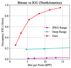
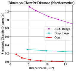
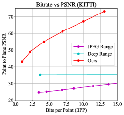
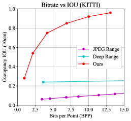
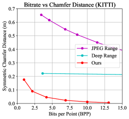
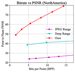
Figure 1: Quantitative results on NorthAmerica and KITTI. From left to right: point-to-plane PSNR, IOU, and Chamfer distance.

We compare against two baselines that use a range image representation of the input point cloud: Deep Range and JPEG Range. Deep Range is the range view-based method discussed in Sec. 4.2 of the main paper. In particular, given a LiDAR point cloud, we first construct a range image by converting it from Euclidean coordinates to polar coordinates, and then storing it as a 2.5D range image. Deep Range then uses a Ballé hyperprior model [1] to compress the 2.5D range image. In contrast, JPEG Range uses the popular JPEG2000 image codec to compress the 2.5D range image.

As shown in Fig. 1, Deep Range outperforms JPEG Range across all reconstruction quality metrics on both NorthAmerica and KITTI. This is a testament to the performance of deep learning-based methods for image compression. Moreover, as we alluded to in Sec. 4.4 of the main paper, our approach significantly outperforms both Deep Range and JPEG Range owing to its use of an octree data structure to represent the LiDAR point cloud and an octree-structured entropy model to compress it.

2.2 Deep Voxel Encoder

We additionally implemented the voxel-based point cloud compression algorithm by Quach et al. [2], consisting of a deep 3D convolutional autoencoder architecture with a fully-factorized entropy model inspired from [1]. We trained and evaluated these models on the NorthAmerica LiDAR point cloud dataset, voxelizing points at (0.25m, 0.25m, 1.0m) for length, width, and depth dimensions respectively. Our best-performing reference model achieves a point-to-plane PSNR of 33.76 at a bitrate of 26.81—this performs much worse than the tree-based methods of Draco (PSNR: 48.47, bpp: 2.778) and our approach (PSNR: 48.95, bpp 1.61). The underperformance of the voxel-based compression method indicates that a dense voxel representation may not be the best fit for compressing LiDAR point clouds due to the inherent sparsity and high frequency information in this data.

3 Runtime

Encoding (ms) Decoding (ms)
Depth Octree Network Range Coding Total Total
11 21.10 13.85 0.80 35.75 92.96
12 23.73 24.67 1.18 49.58 165.70
13 25.51 39.82 2.19 67.52 299.41
14 32.34 56.04 3.15 91.53 486.36
15 34.85 65.17 3.55 103.57 698.98
16 35.52 66.83 3.61 105.96 902.27
Table 4: Runtime of our model with K=4𝐾4K=4 aggregations (in milliseconds). ‘Depth’ is the maximum depth of the octree. ‘Octree’ is the time to build the octree; ‘Network’ the time to run our entropy model; and ‘Range Coding’ the time of range coding.

We benchmarked our approach on a workstation with an Intel Xeon E5-2687W CPU and a Nvidia GeForce GTX 1080 GPU. See Tab. 4 for the results. In our experiments, octree building and range coding were implemented in C++, and our entropy model was implemented in Python with PyTorch. Our approach achieves end-to-end encoding in real-time, meaning that our algorithm can be deployed in an online setting. Moreover, we believe there are many opportunities to speed up our research code significantly, especially in CPU/GPU I/O.

4 Additional Qualitative Results

We exhibit an extensive array of qualitative results that compare our method against Draco across a spectrum of bitrates. In Fig. 2 and 3, we show the reconstruction quality of our method versus Draco. Then, in Fig. 4 and 5, we show their respective downstream semantic segmentation performance. Finally, in Fig. 6, we show their respective downstream object detection performance. As indicated in these figures, our model can attain better results than Draco at comparable—or even lower—bitrates.

5 Change Log

ArXiv v2:

We corrected our definitions of the reconstruction metrics: the symmetric point-to-point Chamfer distance and the symmetric point-to-plane PSNR. We also corrected our estimates of OctSqueeze’s decoding runtime.

\begin{overpic}[width=158.99763pt]{./figures/supplementary_results/54f27a2c-2d88-40a2-ec88-1b583914eedf_116/oracle.jpeg} \put(0.0,55.0){\hbox{\pagecolor{gray!30}\scriptsize GT (NorthAmerica)}} \end{overpic}
\begin{overpic}[width=158.99763pt]{./figures/supplementary_results/54f27a2c-2d88-40a2-ec88-1b583914eedf_116/octree.jpeg} \put(0.0,55.0){\hbox{\pagecolor{gray!30}\scriptsize Ours: PSNR 73.08, Bitrate: 12.23}} \end{overpic}
\begin{overpic}[width=158.99763pt]{./figures/supplementary_results/54f27a2c-2d88-40a2-ec88-1b583914eedf_116/draco.jpeg} \put(0.0,55.0){\hbox{\pagecolor{gray!30}\scriptsize Draco: PSNR 69.81, Bitrate: 12.41}} \end{overpic}
\begin{overpic}[width=158.99763pt]{./figures/supplementary_results/0ea2b29d-2577-4fa7-d85d-3d481a6ebbdb_140/oracle.jpeg} \put(0.0,55.0){\hbox{\pagecolor{gray!30}\scriptsize GT (NorthAmerica)}} \end{overpic}
\begin{overpic}[width=158.99763pt]{./figures/supplementary_results/0ea2b29d-2577-4fa7-d85d-3d481a6ebbdb_140/octree.jpeg} \put(0.0,55.0){\hbox{\pagecolor{gray!30}\scriptsize Ours: PSNR 68.42, Bitrate: 9.38}} \end{overpic}
\begin{overpic}[width=158.99763pt]{./figures/supplementary_results/0ea2b29d-2577-4fa7-d85d-3d481a6ebbdb_140/draco.jpeg} \put(0.0,55.0){\hbox{\pagecolor{gray!30}\scriptsize Draco: PSNR 67.59, Bitrate: 10.42}} \end{overpic}
\begin{overpic}[width=158.99763pt]{./figures/supplementary_results/3d70ca6c-2323-4666-f438-7c24a3bb1510_160/oracle.jpeg} \put(0.0,55.0){\hbox{\pagecolor{gray!30}\scriptsize GT (NorthAmerica)}} \end{overpic}
\begin{overpic}[width=158.99763pt]{./figures/supplementary_results/3d70ca6c-2323-4666-f438-7c24a3bb1510_160/octree.jpeg} \put(0.0,55.0){\hbox{\pagecolor{gray!30}\scriptsize Ours: PSNR 62.48, Bitrate: 7.49}} \end{overpic}
\begin{overpic}[width=158.99763pt]{./figures/supplementary_results/3d70ca6c-2323-4666-f438-7c24a3bb1510_160/draco.jpeg} \put(0.0,55.0){\hbox{\pagecolor{gray!30}\scriptsize Draco: PSNR 58.85, Bitrate: 7.55}} \end{overpic}
\begin{overpic}[width=158.99763pt]{./figures/supplementary_results/007517f3-37ba-4c9e-d54f-a2efc47beab6_027/oracle.jpeg} \put(0.0,55.0){\hbox{\pagecolor{gray!30}\scriptsize GT (NorthAmerica)}} \end{overpic}
\begin{overpic}[width=158.99763pt]{./figures/supplementary_results/007517f3-37ba-4c9e-d54f-a2efc47beab6_027/octree.jpeg} \put(0.0,55.0){\hbox{\pagecolor{gray!30}\scriptsize Ours: PSNR 71.94, Bitrate: 4.63}} \end{overpic}
\begin{overpic}[width=158.99763pt]{./figures/supplementary_results/007517f3-37ba-4c9e-d54f-a2efc47beab6_027/draco.jpeg} \put(0.0,55.0){\hbox{\pagecolor{gray!30}\scriptsize Draco: PSNR 71.03, Bitrate: 6.02}} \end{overpic}
\begin{overpic}[width=158.99763pt]{./figures/supplementary_results/007517f3-37ba-4c9e-d54f-a2efc47beab6_101/oracle.jpeg} \put(0.0,55.0){\hbox{\pagecolor{gray!30}\scriptsize GT (NorthAmerica)}} \end{overpic}
\begin{overpic}[width=158.99763pt]{./figures/supplementary_results/007517f3-37ba-4c9e-d54f-a2efc47beab6_101/octree.jpeg} \put(0.0,55.0){\hbox{\pagecolor{gray!30}\scriptsize Ours: PSNR 46.49, Bitrate: 2.66}} \end{overpic}
\begin{overpic}[width=158.99763pt]{./figures/supplementary_results/007517f3-37ba-4c9e-d54f-a2efc47beab6_101/draco.jpeg} \put(0.0,55.0){\hbox{\pagecolor{gray!30}\scriptsize Draco: PSNR 45.49, Bitrate: 3.95}} \end{overpic}
\begin{overpic}[width=158.99763pt]{./figures/supplementary_results/007517f3-37ba-4c9e-d54f-a2efc47beab6_237/oracle.jpeg} \put(0.0,55.0){\hbox{\pagecolor{gray!30}\scriptsize GT (NorthAmerica)}} \end{overpic}
\begin{overpic}[width=158.99763pt]{./figures/supplementary_results/007517f3-37ba-4c9e-d54f-a2efc47beab6_237/octree.jpeg} \put(0.0,55.0){\hbox{\pagecolor{gray!30}\scriptsize Ours: PSNR 48.61, Bitrate: 1.53}} \end{overpic}
\begin{overpic}[width=158.99763pt]{./figures/supplementary_results/007517f3-37ba-4c9e-d54f-a2efc47beab6_237/draco.jpeg} \put(0.0,55.0){\hbox{\pagecolor{gray!30}\scriptsize Draco: PSNR 47.28, Bitrate: 2.73}} \end{overpic}
Refer to caption
Figure 2: Qualitative results of reconstruction quality for NorthAmerica.
\begin{overpic}[width=158.99763pt]{./figures/supplementary_results/02_001719/oracle.jpeg} \put(0.0,55.0){\hbox{\pagecolor{gray!30}\scriptsize GT (KITTI)}} \end{overpic}
\begin{overpic}[width=158.99763pt]{./figures/supplementary_results/02_001719/octree.jpeg} \put(0.0,55.0){\hbox{\pagecolor{gray!30}\scriptsize Ours: PSNR 65.29, Bitrate: 12.78}} \end{overpic}
\begin{overpic}[width=158.99763pt]{./figures/supplementary_results/02_001719/draco.jpeg} \put(0.0,55.0){\hbox{\pagecolor{gray!30}\scriptsize Draco: PSNR 62.46, Bitrate: 12.90}} \end{overpic}
\begin{overpic}[width=158.99763pt]{./figures/supplementary_results/00_000219/oracle.jpeg} \put(0.0,55.0){\hbox{\pagecolor{gray!30}\scriptsize GT (KITTI)}} \end{overpic}
\begin{overpic}[width=158.99763pt]{./figures/supplementary_results/00_000219/octree.jpeg} \put(0.0,55.0){\hbox{\pagecolor{gray!30}\scriptsize Ours: PSNR 69.99, Bitrate: 9.37}} \end{overpic}
\begin{overpic}[width=158.99763pt]{./figures/supplementary_results/00_000219/draco.jpeg} \put(0.0,55.0){\hbox{\pagecolor{gray!30}\scriptsize Draco: PSNR 66.64, Bitrate: 9.40}} \end{overpic}
\begin{overpic}[width=158.99763pt]{./figures/supplementary_results/08_002401/oracle.jpeg} \put(0.0,55.0){\hbox{\pagecolor{gray!30}\scriptsize GT (KITTI)}} \end{overpic}
\begin{overpic}[width=158.99763pt]{./figures/supplementary_results/08_002401/octree.jpeg} \put(0.0,55.0){\hbox{\pagecolor{gray!30}\scriptsize Ours: PSNR 57.59, Bitrate: 5.23}} \end{overpic}
\begin{overpic}[width=158.99763pt]{./figures/supplementary_results/08_002401/draco.jpeg} \put(0.0,55.0){\hbox{\pagecolor{gray!30}\scriptsize Draco: PSNR 53.42, Bitrate: 5.29}} \end{overpic}
\begin{overpic}[width=158.99763pt]{./figures/supplementary_results/06_000465/oracle.jpeg} \put(0.0,55.0){\hbox{\pagecolor{gray!30}\scriptsize GT (KITTI)}} \end{overpic}
\begin{overpic}[width=158.99763pt]{./figures/supplementary_results/06_000465/octree.jpeg} \put(0.0,55.0){\hbox{\pagecolor{gray!30}\scriptsize Ours: PSNR 52.41, Bitrate: 4.82}} \end{overpic}
\begin{overpic}[width=158.99763pt]{./figures/supplementary_results/06_000465/draco.jpeg} \put(0.0,55.0){\hbox{\pagecolor{gray!30}\scriptsize Draco: PSNR 48.00, Bitrate: 4.88}} \end{overpic}
\begin{overpic}[width=158.99763pt]{./figures/supplementary_results/08_002957/oracle.jpeg} \put(0.0,55.0){\hbox{\pagecolor{gray!30}\scriptsize GT (KITTI)}} \end{overpic}
\begin{overpic}[width=158.99763pt]{./figures/supplementary_results/08_002957/octree.jpeg} \put(0.0,55.0){\hbox{\pagecolor{gray!30}\scriptsize Ours: PSNR 55.06, Bitrate: 2.41}} \end{overpic}
\begin{overpic}[width=158.99763pt]{./figures/supplementary_results/08_002957/draco.jpeg} \put(0.0,55.0){\hbox{\pagecolor{gray!30}\scriptsize Draco: PSNR 50.24, Bitrate: 2.75}} \end{overpic}
\begin{overpic}[width=158.99763pt]{./figures/supplementary_results/07_000777/oracle.jpeg} \put(0.0,55.0){\hbox{\pagecolor{gray!30}\scriptsize GT (KITTI)}} \end{overpic}
\begin{overpic}[width=158.99763pt]{./figures/supplementary_results/07_000777/octree.jpeg} \put(0.0,55.0){\hbox{\pagecolor{gray!30}\scriptsize Ours: PSNR 43.67, Bitrate: 1.52}} \end{overpic}
\begin{overpic}[width=158.99763pt]{./figures/supplementary_results/07_000777/draco.jpeg} \put(0.0,55.0){\hbox{\pagecolor{gray!30}\scriptsize Draco: PSNR 39.09, Bitrate: 2.04}} \end{overpic}
Refer to caption
Figure 3: Qualitative results of reconstruction quality for KITTI.
\begin{overpic}[width=158.99763pt]{./figures/downstream_results/supplemental_visualizations/kitti_seg/08_3013_oracle.jpeg} \put(0.0,55.0){\hbox{\pagecolor{gray!30}\scriptsize Oracle: IOU 40.86, Bitrate: 96.00}} \end{overpic}
\begin{overpic}[width=158.99763pt]{./figures/downstream_results/supplemental_visualizations/kitti_seg/08_3013_octree16.jpeg} \put(0.0,55.0){\hbox{\pagecolor{gray!30}\scriptsize Ours: IOU 39.10, Bitrate: 13.37}} \end{overpic}
\begin{overpic}[width=158.99763pt]{./figures/downstream_results/supplemental_visualizations/kitti_seg/08_3013_draco15.jpeg} \put(0.0,55.0){\hbox{\pagecolor{gray!30}\scriptsize Draco: IOU 38.98, Bitrate: 15.63}} \end{overpic}
\begin{overpic}[width=158.99763pt]{./figures/downstream_results/supplemental_visualizations/kitti_seg/08_3021_oracle.jpeg} \put(0.0,55.0){\hbox{\pagecolor{gray!30}\scriptsize Oracle: IOU 38.39, Bitrate: 96.00}} \end{overpic}
\begin{overpic}[width=158.99763pt]{./figures/downstream_results/supplemental_visualizations/kitti_seg/08_3021_octree15.jpeg} \put(0.0,55.0){\hbox{\pagecolor{gray!30}\scriptsize Ours: IOU 36.70, Bitrate: 10.37}} \end{overpic}
\begin{overpic}[width=158.99763pt]{./figures/downstream_results/supplemental_visualizations/kitti_seg/08_3021_draco14.jpeg} \put(0.0,55.0){\hbox{\pagecolor{gray!30}\scriptsize Draco: IOU 35.61, Bitrate: 12.70}} \end{overpic}
\begin{overpic}[width=158.99763pt]{./figures/downstream_results/supplemental_visualizations/kitti_seg/08_2807_oracle.jpeg} \put(0.0,55.0){\hbox{\pagecolor{gray!30}\scriptsize Oracle: IOU 35.52, Bitrate: 96.00}} \end{overpic}
\begin{overpic}[width=158.99763pt]{./figures/downstream_results/supplemental_visualizations/kitti_seg/08_2807_octree14.jpeg} \put(0.0,55.0){\hbox{\pagecolor{gray!30}\scriptsize Ours: IOU 35.75, Bitrate: 6.87}} \end{overpic}
\begin{overpic}[width=158.99763pt]{./figures/downstream_results/supplemental_visualizations/kitti_seg/08_2807_draco13.jpeg} \put(0.0,55.0){\hbox{\pagecolor{gray!30}\scriptsize Draco: IOU 35.08, Bitrate: 9.30}} \end{overpic}
\begin{overpic}[width=158.99763pt]{./figures/downstream_results/supplemental_visualizations/kitti_seg/08_2990_oracle.jpeg} \put(0.0,55.0){\hbox{\pagecolor{gray!30}\scriptsize Oracle: IOU 39.41, Bitrate: 96.00}} \end{overpic}
\begin{overpic}[width=158.99763pt]{./figures/downstream_results/supplemental_visualizations/kitti_seg/08_2990_octree13.jpeg} \put(0.0,55.0){\hbox{\pagecolor{gray!30}\scriptsize Ours: IOU 29.92, Bitrate: 4.70}} \end{overpic}
\begin{overpic}[width=158.99763pt]{./figures/downstream_results/supplemental_visualizations/kitti_seg/08_2990_draco11.jpeg} \put(0.0,55.0){\hbox{\pagecolor{gray!30}\scriptsize Draco: IOU 23.23, Bitrate: 4.70}} \end{overpic}
\begin{overpic}[width=158.99763pt]{./figures/downstream_results/supplemental_visualizations/kitti_seg/08_2319_oracle.jpeg} \put(0.0,55.0){\hbox{\pagecolor{gray!30}\scriptsize Oracle: IOU 35.20, Bitrate: 96.00}} \end{overpic}
\begin{overpic}[width=158.99763pt]{./figures/downstream_results/supplemental_visualizations/kitti_seg/08_2319_octree13.jpeg} \put(0.0,55.0){\hbox{\pagecolor{gray!30}\scriptsize Ours: IOU 26.38, Bitrate: 2.56}} \end{overpic}
\begin{overpic}[width=158.99763pt]{./figures/downstream_results/supplemental_visualizations/kitti_seg/08_2319_draco11.jpeg} \put(0.0,55.0){\hbox{\pagecolor{gray!30}\scriptsize Draco: IOU 21.02, Bitrate: 2.67}} \end{overpic}
\begin{overpic}[width=158.99763pt]{./figures/downstream_results/supplemental_visualizations/kitti_seg/08_3645_oracle.jpeg} \put(0.0,55.0){\hbox{\pagecolor{gray!30}\scriptsize Oracle: IOU 34.81, Bitrate: 96.00}} \end{overpic}
\begin{overpic}[width=158.99763pt]{./figures/downstream_results/supplemental_visualizations/kitti_seg/08_3645_octree12.jpeg} \put(0.0,55.0){\hbox{\pagecolor{gray!30}\scriptsize Ours: IOU 23.04, Bitrate: 1.62}} \end{overpic}
\begin{overpic}[width=158.99763pt]{./figures/downstream_results/supplemental_visualizations/kitti_seg/08_3645_draco10.jpeg} \put(0.0,55.0){\hbox{\pagecolor{gray!30}\scriptsize Draco: IOU 18.55, Bitrate: 1.96}} \end{overpic}
Figure 4: Qualitative results of semantic segmentation for KITTI. IOU is averaged over all classes.
\begin{overpic}[width=158.99763pt]{./figures/downstream_results/supplemental_visualizations/tor4d_seg/39b907e7-f390-4cad-d3a2-0cba4a920f41_245_oracle.jpeg} \put(0.0,55.0){\hbox{\pagecolor{gray!30}\scriptsize Oracle: IOU 99.55, Bitrate: 96.00}} \end{overpic}
\begin{overpic}[width=158.99763pt]{./figures/downstream_results/supplemental_visualizations/tor4d_seg/39b907e7-f390-4cad-d3a2-0cba4a920f41_245_octree16.jpeg} \put(0.0,55.0){\hbox{\pagecolor{gray!30}\scriptsize Ours: IOU 96.77, Bitrate: 14.87}} \end{overpic}
\begin{overpic}[width=158.99763pt]{./figures/downstream_results/supplemental_visualizations/tor4d_seg/39b907e7-f390-4cad-d3a2-0cba4a920f41_245_draco15.jpeg} \put(0.0,55.0){\hbox{\pagecolor{gray!30}\scriptsize Draco: IOU 95.64, Bitrate: 16.46}} \end{overpic}
\begin{overpic}[width=158.99763pt]{./figures/downstream_results/supplemental_visualizations/tor4d_seg/be53e8ce-e5de-45b7-f69d-2312ab9cac0a_135_oracle.jpeg} \put(0.0,55.0){\hbox{\pagecolor{gray!30}\scriptsize Oracle: IOU 97.21, Bitrate: 96.00}} \end{overpic}
\begin{overpic}[width=158.99763pt]{./figures/downstream_results/supplemental_visualizations/tor4d_seg/be53e8ce-e5de-45b7-f69d-2312ab9cac0a_135_octree15.jpeg} \put(0.0,55.0){\hbox{\pagecolor{gray!30}\scriptsize Ours: IOU 92.50, Bitrate: 11.68}} \end{overpic}
\begin{overpic}[width=158.99763pt]{./figures/downstream_results/supplemental_visualizations/tor4d_seg/be53e8ce-e5de-45b7-f69d-2312ab9cac0a_135_draco14.jpeg} \put(0.0,55.0){\hbox{\pagecolor{gray!30}\scriptsize Draco: IOU 91.28, Bitrate: 12.95}} \end{overpic}
\begin{overpic}[width=158.99763pt]{./figures/downstream_results/supplemental_visualizations/tor4d_seg/4f8665f1-5ca5-4e71-eeef-876feedf4dc3_180_oracle.jpeg} \put(0.0,55.0){\hbox{\pagecolor{gray!30}\scriptsize Oracle: IOU 98.09, Bitrate: 96.00}} \end{overpic}
\begin{overpic}[width=158.99763pt]{./figures/downstream_results/supplemental_visualizations/tor4d_seg/4f8665f1-5ca5-4e71-eeef-876feedf4dc3_180_octree14.jpeg} \put(0.0,55.0){\hbox{\pagecolor{gray!30}\scriptsize Ours: IOU 86.44, Bitrate: 8.62}} \end{overpic}
\begin{overpic}[width=158.99763pt]{./figures/downstream_results/supplemental_visualizations/tor4d_seg/4f8665f1-5ca5-4e71-eeef-876feedf4dc3_180_draco13.jpeg} \put(0.0,55.0){\hbox{\pagecolor{gray!30}\scriptsize Draco: IOU 82.93, Bitrate: 10.21}} \end{overpic}
\begin{overpic}[width=158.99763pt]{./figures/downstream_results/supplemental_visualizations/tor4d_seg/bf4c4374-d1a6-4c1e-d32a-25d726eed474_150_oracle.jpeg} \put(0.0,55.0){\hbox{\pagecolor{gray!30}\scriptsize Oracle: IOU 98.01, Bitrate: 96.00}} \end{overpic}
\begin{overpic}[width=158.99763pt]{./figures/downstream_results/supplemental_visualizations/tor4d_seg/bf4c4374-d1a6-4c1e-d32a-25d726eed474_150_octree13.jpeg} \put(0.0,55.0){\hbox{\pagecolor{gray!30}\scriptsize Ours: IOU 81.95, Bitrate: 5.52}} \end{overpic}
\begin{overpic}[width=158.99763pt]{./figures/downstream_results/supplemental_visualizations/tor4d_seg/bf4c4374-d1a6-4c1e-d32a-25d726eed474_150_draco12.jpeg} \put(0.0,55.0){\hbox{\pagecolor{gray!30}\scriptsize Draco: IOU 80.61, Bitrate: 6.99}} \end{overpic}
\begin{overpic}[width=158.99763pt]{./figures/downstream_results/supplemental_visualizations/tor4d_seg/4a7b1d02-2bd7-4763-e2bd-a051332be0c1_100_oracle.jpeg} \put(0.0,55.0){\hbox{\pagecolor{gray!30}\scriptsize Oracle: IOU 92.31, Bitrate: 96.00}} \end{overpic}
\begin{overpic}[width=158.99763pt]{./figures/downstream_results/supplemental_visualizations/tor4d_seg/4a7b1d02-2bd7-4763-e2bd-a051332be0c1_100_octree12.jpeg} \put(0.0,55.0){\hbox{\pagecolor{gray!30}\scriptsize Ours: IOU 58.62, Bitrate: 2.67}} \end{overpic}
\begin{overpic}[width=158.99763pt]{./figures/downstream_results/supplemental_visualizations/tor4d_seg/4a7b1d02-2bd7-4763-e2bd-a051332be0c1_100_draco11.jpeg} \put(0.0,55.0){\hbox{\pagecolor{gray!30}\scriptsize Draco: IOU 57.18, Bitrate: 3.99}} \end{overpic}
\begin{overpic}[width=158.99763pt]{./figures/downstream_results/supplemental_visualizations/tor4d_seg/4ef8b66b-2e7b-43a9-d13f-cfc6c3bb4d28_215_oracle.jpeg} \put(0.0,55.0){\hbox{\pagecolor{gray!30}\scriptsize Oracle: IOU 95.53, Bitrate: 96.00}} \end{overpic}
\begin{overpic}[width=158.99763pt]{./figures/downstream_results/supplemental_visualizations/tor4d_seg/4ef8b66b-2e7b-43a9-d13f-cfc6c3bb4d28_215_octree11.jpeg} \put(0.0,55.0){\hbox{\pagecolor{gray!30}\scriptsize Ours: IOU 30.87, Bitrate: 1.78}} \end{overpic}
\begin{overpic}[width=158.99763pt]{./figures/downstream_results/supplemental_visualizations/tor4d_seg/4ef8b66b-2e7b-43a9-d13f-cfc6c3bb4d28_215_draco10.jpeg} \put(0.0,55.0){\hbox{\pagecolor{gray!30}\scriptsize Draco: IOU 25.28, Bitrate: 2.90}} \end{overpic}
Figure 5: Qualitative results of semantic segmentation for NorthAmerica. IOU is averaged over all classes.
\begin{overpic}[width=158.99763pt]{./figures/downstream_results/supplemental_visualizations/tor4d_det/aee39080-edc7-4773-dd2f-9d9657011dbe_155_oracle.jpeg} \put(0.0,55.0){\hbox{\pagecolor{gray!30}\scriptsize Oracle: AP: 93.02, Bitrate: 96.00}} \end{overpic}
\begin{overpic}[width=158.99763pt]{./figures/downstream_results/supplemental_visualizations/tor4d_det/aee39080-edc7-4773-dd2f-9d9657011dbe_155_octree16.jpeg} \put(0.0,55.0){\hbox{\pagecolor{gray!30}\scriptsize Ours: AP: 93.00, Bitrate: 14.64}} \end{overpic}
\begin{overpic}[width=158.99763pt]{./figures/downstream_results/supplemental_visualizations/tor4d_det/aee39080-edc7-4773-dd2f-9d9657011dbe_155_draco16.jpeg} \put(0.0,55.0){\hbox{\pagecolor{gray!30}\scriptsize Draco: AP: 92.78, Bitrate: 18.87}} \end{overpic}
\begin{overpic}[width=158.99763pt]{./figures/downstream_results/supplemental_visualizations/tor4d_det/2c3e4798-33c2-46fb-da63-d566660d6131_125_oracle.jpeg} \put(0.0,55.0){\hbox{\pagecolor{gray!30}\scriptsize Oracle: AP: 88.49, Bitrate: 96.00}} \end{overpic}
\begin{overpic}[width=158.99763pt]{./figures/downstream_results/supplemental_visualizations/tor4d_det/2c3e4798-33c2-46fb-da63-d566660d6131_125_octree15.jpeg} \put(0.0,55.0){\hbox{\pagecolor{gray!30}\scriptsize Ours: AP: 88.06, Bitrate: 10.72}} \end{overpic}
\begin{overpic}[width=158.99763pt]{./figures/downstream_results/supplemental_visualizations/tor4d_det/2c3e4798-33c2-46fb-da63-d566660d6131_125_draco14.jpeg} \put(0.0,55.0){\hbox{\pagecolor{gray!30}\scriptsize Draco: AP: 88.27, Bitrate: 11.97}} \end{overpic}
\begin{overpic}[width=158.99763pt]{./figures/downstream_results/supplemental_visualizations/tor4d_det/ccfdd1fe-2eed-4c29-eee1-826a9ba893ed_225_oracle.jpeg} \put(0.0,55.0){\hbox{\pagecolor{gray!30}\scriptsize Oracle: AP: 87.85, Bitrate: 96.00}} \end{overpic}
\begin{overpic}[width=158.99763pt]{./figures/downstream_results/supplemental_visualizations/tor4d_det/ccfdd1fe-2eed-4c29-eee1-826a9ba893ed_225_octree14.jpeg} \put(0.0,55.0){\hbox{\pagecolor{gray!30}\scriptsize Ours: AP: 87.50, Bitrate: 8.52}} \end{overpic}
\begin{overpic}[width=158.99763pt]{./figures/downstream_results/supplemental_visualizations/tor4d_det/ccfdd1fe-2eed-4c29-eee1-826a9ba893ed_225_draco13.jpeg} \put(0.0,55.0){\hbox{\pagecolor{gray!30}\scriptsize Draco: AP: 86.95, Bitrate: 10.16}} \end{overpic}
\begin{overpic}[width=158.99763pt]{./figures/downstream_results/supplemental_visualizations/tor4d_det/df3e28ad-f124-4b73-d56a-8e0d773ec213_130_oracle.jpeg} \put(0.0,55.0){\hbox{\pagecolor{gray!30}\scriptsize Oracle: AP: 89.79, Bitrate: 96.00}} \end{overpic}
\begin{overpic}[width=158.99763pt]{./figures/downstream_results/supplemental_visualizations/tor4d_det/df3e28ad-f124-4b73-d56a-8e0d773ec213_130_octree13.jpeg} \put(0.0,55.0){\hbox{\pagecolor{gray!30}\scriptsize Ours: AP: 89.39, Bitrate: 5.51}} \end{overpic}
\begin{overpic}[width=158.99763pt]{./figures/downstream_results/supplemental_visualizations/tor4d_det/df3e28ad-f124-4b73-d56a-8e0d773ec213_130_draco12.jpeg} \put(0.0,55.0){\hbox{\pagecolor{gray!30}\scriptsize Draco: AP: 89.26, Bitrate: 6.94}} \end{overpic}
\begin{overpic}[width=158.99763pt]{./figures/downstream_results/supplemental_visualizations/tor4d_det/86995fc8-a49f-453a-fe6d-14df9c181aab_080_oracle.jpeg} \put(0.0,55.0){\hbox{\pagecolor{gray!30}\scriptsize Oracle: AP: 86.71, Bitrate: 96.00}} \end{overpic}
\begin{overpic}[width=158.99763pt]{./figures/downstream_results/supplemental_visualizations/tor4d_det/86995fc8-a49f-453a-fe6d-14df9c181aab_080_octree12.jpeg} \put(0.0,55.0){\hbox{\pagecolor{gray!30}\scriptsize Ours: AP: 86.17, Bitrate: 3.39}} \end{overpic}
\begin{overpic}[width=158.99763pt]{./figures/downstream_results/supplemental_visualizations/tor4d_det/86995fc8-a49f-453a-fe6d-14df9c181aab_080_draco11.jpeg} \put(0.0,55.0){\hbox{\pagecolor{gray!30}\scriptsize Draco: AP: 85.27, Bitrate: 5.00}} \end{overpic}
\begin{overpic}[width=158.99763pt]{./figures/downstream_results/supplemental_visualizations/tor4d_det/be53e8ce-e5de-45b7-f69d-2312ab9cac0a_030_oracle.jpeg} \put(0.0,55.0){\hbox{\pagecolor{gray!30}\scriptsize Oracle: AP: 88.08, Bitrate: 96.00}} \end{overpic}
\begin{overpic}[width=158.99763pt]{./figures/downstream_results/supplemental_visualizations/tor4d_det/be53e8ce-e5de-45b7-f69d-2312ab9cac0a_030_octree11.jpeg} \put(0.0,55.0){\hbox{\pagecolor{gray!30}\scriptsize Ours: AP: 87.30, Bitrate: 1.39}} \end{overpic}
\begin{overpic}[width=158.99763pt]{./figures/downstream_results/supplemental_visualizations/tor4d_det/be53e8ce-e5de-45b7-f69d-2312ab9cac0a_030_draco10.jpeg} \put(0.0,55.0){\hbox{\pagecolor{gray!30}\scriptsize Draco: AP: 83.80, Bitrate: 2.42}} \end{overpic}
Figure 6: Qualitative results of object detection for NorthAmerica. AP is averaged over vehicle, motorbike, and pedestrian classes.

References

  • [1] Johannes Ballé, David Minnen, Saurabh Singh, Sung Jin Hwang, and Nick Johnston. Variational image compression with a scale hyperprior. In 6th International Conference on Learning Representations, ICLR 2018, Vancouver, BC, Canada, April 30 - May 3, 2018, Conference Track Proceedings. OpenReview.net, 2018.
  • [2] Maurice Quach, Giuseppe Valenzise, and Frédéric Dufaux. Learning convolutional transforms for lossy point cloud geometry compression. In 2019 IEEE International Conference on Image Processing, ICIP 2019, Taipei, Taiwan, September 22-25, 2019, pages 4320–4324. IEEE, 2019.