On the derivatives of feed-forward neural networks

Abstract

In this paper we present a C++ implementation of the analytic derivative of a feed-forward neural network with respect to its free parameters for an arbitrary architecture, known as back-propagation. We dubbed this code NNAD (Neural Network Analytic Derivatives) and interfaced it with the widely-used ceres-solver [1] minimiser to fit neural networks to pseudodata in two different least-squares problems. The first is a direct fit of Legendre polynomials. The second is a somewhat more involved minimisation problem where the function to be fitted takes part in an integral. Finally, using a consistent framework, we assess the efficiency of our analytic derivative formula as compared to numerical and automatic differentiation as provided by ceres-solver. We thus demonstrate the advantage of using NNAD in problems involving both deep or shallow neural networks.

figuresection

Nikhef/2020-011

PROGRAM SUMMARY

Program Title: NNAD
Licensing provisions: MIT
Programming language: C++
Nature of problem: computation of the gradient of a feed-forward neural network with respect to its parameters (weights and biases). This is a proxy for the computation of the gradient of sensible figures of merit used in optimisation problems.
Solution method: analytic derivative of a feed-forward neural network with arbitrary architecture by means of a recursive application of the chain rule.

1 Introduction

The extraction of information from experimental measurements often requires parametrising some relevant quantities using suitable functional forms that are eventually fitted to the data. In many cases, even the general behaviour of such quantities is largely unknown. In order to avoid unwanted parametric biases, it is convenient to make as few assumptions as possible on the associated functional form. This requires flexible objects able to describe a large variety of behaviours: neural networks (NNs) are thus suitable candidates (see, e.g., Refs. [2, 3, 4] for some applications in high-energy physics). However, the flexibility of NNs comes at the cost of a complex multidimensional parameter space. Therefore, fitting (or training) a NN typically requires a heavy numerical effort aimed at finding the best fit parameters in a very complicated parameter space.

Efficient training algorithms often rely on the knowledge of the gradient in parameter space of the figure of merit chosen to measure the goodness of the fit. Therefore, an efficient computation of the gradient is crucial to achieve performance. This is especially true for complicated figures of merit involving NNs.

There are fundamentally two main approaches to the computation of a gradient. The first is the numerical approach. The second is the analytic approach that can be further branched off into: “fully” analytic (henceforth simply analytic) and automatic differentiations (See Sect. 5 for more details).

In this paper we consider feed-forward NNs with arbitrary architecture and derive a compact back-propagation algorithm to analytically compute their gradient in parameter space. We then implement this algorithm in a C++ code and compare it to numerical and automatic differentiation as implemented in ceres-solver [1].

The paper is organised as follows. In Sect. 2, we first define the figure of merit that we will use throughout the paper and then derive the analytic back-propagation algorithm (NNAD) for a feed-forward NN. In Sect. 4, we use NNAD in two specific cases: 1) a fit of pseudodata generated using a Legendre polynomial and 2) a fit of functions involved in convolution integrals. We devote Sect. 5 to assess the performance of our algorithm as compared to numerical and automatic differentiations. Finally, we give some conclusive remarks in Sect. 6. A provides some details concerning the main functionalities of the C++ implementation.

2 Definition and optimisation of the figure of merit

In this section we define the particular figure of merit that we will be using throughout the paper. The figure of merit has the purpose of “measuring” the degree of agreement between a set of data and some parametric model. A common choice for the figure of merit is the likelihood function.

The likelihood function can be defined as the probability of observing a given sample of data for a given set of parameters of the given model. Let $\bm{D}=\{D_{1},D_{2},...D_{n}\}$ be a set of random variables having a joint probability density $\mathcal{F}$ depending on a set of parameters $\bm{\theta}=\{\theta_{1},\theta_{2},...,\theta_{m}\}$ of some parametric model. From the definition above, one can write the likelihood function as:

$$\mathcal{L}(\bm{\theta}|\bm{d})=\mathcal{F}_{\bm{\theta}}(\bm{d})\equiv\prod_{i}^{n}f_{i,\bm{\theta}}(d_{i})\,,$$ (1)

where $\bm{d}=\{d_{1},d_{2},...,d_{n}\}$ are the observed values of $\bm{D}$ (the data) and $f_{i,\bm{\theta}}$ is the single probability distribution of $D_{i}$ given the set of parameters $\bm{\theta}$. Let us take all $f_{i}$ to be mutually independent normal distributions, therefore:

$$\mathcal{L}(\bm{\theta}|\bm{d})=\prod_{i}^{n}\frac{1}{\sqrt{2\pi\sigma_{i}^{2}}}e^{-\frac{(m_{i}({\bm{\theta}})-d_{i})^{2}}{2\sigma_{i}^{2}}}\,,$$ (2)

where $d_{i}$ and $\sigma_{i}$ are respectively the central value and the uncertainty of the $i$-th datapoint, and $m_{i}$ is the corresponding model prediction obtained with the set of parameters $\bm{\theta}$.

The goal of a regression analysis is to find a particular set of parameters $\bm{\theta}$ that maximises the likelihood $\mathcal{L}(\bm{\theta})$, thus maximising the probability of observing the given data. This procedure typically goes under the name of maximum likelihood estimation. However, finding the maximum of the likelihood turns out to be computationally expensive. In order to simplify the problem, one can equivalently maximise the logarithm of the likelihood, that reads:

$$\ln\left(\mathcal{L}(\bm{\theta}|\bm{d})\right)=-\frac{n}{2}\ln{(2\pi)}+\sum_{i}^{n}\ln{\frac{1}{\sigma_{i}}}-\frac{1}{2}\sum_{i}^{n}\left(\frac{m_{i}(\bm{\theta})-d_{i}}{\sigma_{i}}\right)^{2}\,.$$ (3)

Since the first two terms on the right-hand side are constant and the last term is negative, maximising the likelihood is equivalent to minimising this last term, that is:

$$\max_{\bm{\theta}}\ln\left(\mathcal{L}(\bm{\theta}|\bm{d})\right)\rightarrow\min_{\bm{\theta}}\sum^{n}_{i}\left(\frac{m_{i}(\bm{\theta})-d_{i}}{\sigma_{i}}\right)^{2}\equiv\min_{\bm{\theta}}\chi^{2}(\bm{\theta})\,.$$ (4)

This defines the $\chi^{2}$ as an effective loss function to be minimised in a regression analysis. In the studies below, we will use the $\chi^{2}$ as a figure of merit.

There exist numerous strategies to solve Eq. (4). In this paper we will focus on deterministic derivative-based algorithms whereby the solution of Eq. (4) is reached by following the steepest descending path on the hyper-surface defined by the $\chi^{2}$. Alternatives to the deterministic approach are the derivative-free algorithms that broadly consist of exploring random paths of the parameter space until the minimum of the $\chi^{2}$ is found. Examples of derivative-free algorithms are the genetic algorithm and the covariance-matrix-adaptation evolution-strategy [5].

Within deterministic derivative-based algorithms, we have chosen to work with the quite popular Levenberg-Marquardt algorithm [6]. It combines the gradient-descent algorithm to the Gauss-Newton method. When the parameters are far from their optimal value, the Levenberg-Marquardt method behaves more like a gradient-descent algorithm in which the $\chi^{2}$ is reduced by updating the parameters along the steepest-descent direction. The Gauss-Newton method is instead used when the parameters are close to their optimal value to identify the minimum of the $\chi^{2}$ by assuming it to be locally quadratic. Both the gradient-descent and Gauss-Newton methods rely on the knowledge of the derivatives of the $\chi^{2}$ with respect to the parameters $\bm{\theta}$. In fact, the computation of the gradient of the $\chi^{2}$ is a bottleneck for all deterministic algorithms in general and, as such, for the Levenberg-Marquardt one in particular. Therefore, an efficient computation of this quantity is highly desirable.

3 Derivative of the $\chi^{2}$

In this section we discuss how to treat the gradient of the $\chi^{2}$ for a model parameterised by a feed-forward NN. This will automatically result into the derivative of the NN itself that we will then explicitly work out.

For the sake of simplicity, we consider one single experimental point measured at ${\boldsymbol{\xi}}\in\mathbb{R}^{m}$ with central value ${\boldsymbol{d}}\in\mathbb{R}^{n}$ and standard deviation $\boldsymbol{\sigma}\in\mathbb{R}^{n}$ that we want to fit with a NN ${\boldsymbol{N}}:\mathbb{R}^{m}\rightarrow\mathbb{R}^{n}$ with $L$ layers and parametrised by a set of weights and biases $\{\omega_{ij}^{(\ell)},\theta_{i}^{(\ell)}\}$. The corresponding $\chi^{2}$ reads:

$$\chi^{2}[\{\omega_{ij}^{(\ell)},\theta_{i}^{(\ell)}\}]=\sum_{k=1}^{n}\left(\frac{N_{k}({\boldsymbol{\xi}};\{\omega_{ij}^{(\ell)},\theta_{i}^{(\ell)}\})-d_{k}}{\sigma_{k}}\right)^{2}\,,$$ (5)

where $N_{k}$ is the $k$-th output of the NN. We also assume that all the nodes belonging to the $\ell$-th layer have the same activation function $\phi_{\ell}$. The $k$-th output of the NN can then be written recursively as:

$$\begin{array}[]{rcl}\displaystyle N_{k}({\boldsymbol{\xi}};\{\omega_{ij}^{(\ell)},\theta_{i}^{(\ell)}\})&=&\displaystyle\phi_{L}\left(\sum_{j^{(1)}}^{N_{L-1}}\omega_{kj^{(1)}}^{(L)}y_{j^{(1)}}^{(L-1)}+\theta_{k}^{(L)}\right)\\ \\ &=&\displaystyle\phi_{L}\left(\sum_{j^{(1)}=1}^{N_{L-1}}\omega_{kj^{(1)}}^{(L)}\phi_{L-1}\left(\sum_{j^{(2)}=1}^{N_{L-2}}\omega_{j^{(1)}j^{(2)}}^{(L)}y_{j^{(2)}}^{(L-2)}+\theta_{j^{(1)}}^{(L-1)}\right)+\theta_{k}^{(L)}\right)\\ &=&\dots\,.\end{array}$$ (6)

The nesting in Eq. (6) continues until the input layer is reached. The derivative of the $\chi^{2}$ in Eq. (5) with respect to the weight $\omega_{ij}^{(\ell)}$, relevant to the computation of the gradient, takes the form:

$$\frac{\partial\chi^{2}}{\partial\omega_{ij}^{(\ell)}}=2\sum_{k=1}^{n}\left(\frac{N_{k}({\boldsymbol{\xi}};\{\omega_{ij}^{(\ell)},\theta_{i}^{(\ell)}\})-d_{k}}{\sigma_{k}^{2}}\right)\frac{\partial N_{k}}{\partial\omega_{ij}^{(\ell)}}\,,$$ (7)

and similarly for the derivative with respect to the bias $\theta_{i}^{(\ell)}$. Eq. (7) reduces the computation of the derivatives of the $\chi^{2}$ in Eq. (5) to the computation of the derivatives of ${\boldsymbol{N}}$. In this respect, the feed-forward structure of the NN in Eq. (6) is crucial to work out an explicit expression for such derivatives. We start by defining:

$$\begin{array}[]{l}\displaystyle x_{i}^{(\ell)}=\sum_{j=1}^{N_{\ell-1}}\omega_{ij}^{(\ell)}y_{j}^{(\ell-1)}+\theta_{i}^{(\ell)}\,,\\ \\ \displaystyle y_{i}^{(\ell)}=\phi_{\ell}\left(x_{i}^{(\ell)}\right)\,,\\ \\ \displaystyle z_{i}^{(\ell)}=\phi^{\prime}_{\ell}\left(x_{i}^{(\ell)}\right)\,.\end{array}$$ (8)

We then apply the chain rule to compute the derivative of $N_{k}$ w.r.t. $\omega_{ij}^{(\ell)}$:

$$\begin{array}[]{rcl}\displaystyle\frac{\partial N_{k}}{\partial\omega_{ij}^{(\ell)}}&=&\displaystyle\frac{\partial y_{k}^{(L)}}{\partial\omega_{ij}^{(\ell)}}\\ \\ &=&\displaystyle z_{k}^{(L)}\frac{\partial x_{k}^{(L)}}{\partial\omega_{ij}^{(\ell)}}\\ \\ &=&\displaystyle\sum_{j^{(1)}=1}^{N_{L-1}}\left[z_{k}^{(L)}\omega_{kj^{(1)}}^{(L)}\right]\frac{\partial y_{j^{(1)}}^{(L-1)}}{\partial\omega_{ij}^{(\ell)}}\\ \\ &=&\displaystyle\sum_{j^{(1)}=1}^{N_{L-1}}\sum_{j^{(2)}=1}^{N_{L-2}}\left[z_{k}^{(L)}\omega_{kj^{(1)}}^{(L)}\right]\left[z_{j^{(1)}}^{(L-1)}\omega_{j^{(1)}j^{(2)}}^{(L-1)}\right]\frac{\partial y_{j^{(2)}}^{(L-2)}}{\partial\omega_{ij}^{(\ell)}}\\ \\ &=&\displaystyle\dots\end{array}$$ (9)

As evident, the chain rule penetrates into the NN starting from the output layer all the way back until the $\ell$-th layer (i.e. the layer where the parameter $\omega_{ij}^{(\ell)}$ belongs to). In order to write the derivative in a closed form, we define the $(i,j)$ entry of the matrix $\mathbf{S}^{(\ell)}$ as:

$$z_{i}^{(\ell)}\omega_{ij}^{(\ell)}=S_{ij}^{(\ell)}\left(=\frac{\partial y_{i}^{(\ell)}}{\partial y_{j}^{(\ell-1)}}\right)\,,$$ (10)

so that:

$$\frac{\partial{\boldsymbol{N}}}{\partial\omega_{ij}^{(\ell)}}=\mathbf{S}^{(L)}\cdot\mathbf{S}^{(L-1)}\cdots\mathbf{S}^{(\ell+1)}\cdot\frac{\partial{\boldsymbol{y}}^{(\ell)}}{\partial\omega_{ij}^{(\ell)}}\,,$$ (11)

with ${\boldsymbol{y}}^{(\ell)}$ the $N_{\ell}$-dimensional vector of all $y_{i}^{(\ell)}$. This expression can be written in a more compact form as:

$$\frac{\partial{\boldsymbol{N}}}{\partial\omega_{ij}^{(\ell)}}=\left[\prod_{\alpha=L}^{\ell+1}\mathbf{S}^{(\alpha)}\right]\cdot\frac{\partial{\boldsymbol{y}}^{(\ell)}}{\partial\omega_{ij}^{(\ell)}}\,.$$ (12)

It is important to notice that the product of matrices $\mathbf{S}^{(\alpha)}$ in Eq. (12) runs backwards from $L$ to $\ell+1$. The derivative in the r.h.s. of Eq. (12) can finally be computed explicitly and for the $k$-th component of ${\boldsymbol{y}}^{(\ell)}$ it reads:

$$\frac{\partial y_{k}^{(\ell)}}{\partial\omega_{ij}^{(\ell)}}=z_{k}^{(\ell)}\frac{\partial x_{k}^{(\ell)}}{\partial\omega_{ij}^{(\ell)}}=\delta_{ki}z_{i}^{(\ell)}y_{j}^{(\ell-1)}\,.$$ (13)

Similarly, the derivative of ${\boldsymbol{N}}$ w.r.t. the bias $\theta_{i}^{(\ell)}$ takes the form:

$$\frac{\partial{\boldsymbol{N}}}{\partial\theta_{i}^{(\ell)}}=\left[\prod_{\alpha=L}^{\ell+1}\mathbf{S}^{(\alpha)}\right]\cdot\frac{\partial{\boldsymbol{y}}^{(\ell)}}{\partial\theta_{i}^{(\ell)}}\,,$$ (14)

with:

$$\frac{\partial y_{k}^{(\ell)}}{\partial\theta_{i}^{(\ell)}}=\delta_{ki}z_{i}^{(\ell)}\,.$$ (15)

The presence of $\delta_{ki}$ in both Eqs. (13) and (15) simplifies the computation yielding:

$$\begin{array}[]{rcl}\displaystyle\frac{\partial N_{k}}{\partial\theta_{i}^{(\ell)}}&=&\displaystyle{\Sigma}_{ki}^{(\ell)}z_{i}^{(\ell)}\,,\\ \\ \displaystyle\frac{\partial N_{k}}{\partial\omega_{ij}^{(\ell)}}&=&\displaystyle{\Sigma}_{ki}^{(\ell)}z_{i}^{(\ell)}y_{j}^{(\ell-1)}\,,\end{array}$$ (16)

where ${\Sigma}_{ki}^{(\ell)}$ is the $(k,i)$ entry of the matrix:

$$\mathbf{\Sigma}^{(\ell)}=\prod_{\alpha=L}^{\ell+1}\mathbf{S}^{(\alpha)}\,.$$ (17)

The identities in Eq. (16) can finally be used to compute the gradient of the $\chi^{2}$ through Eq. (7) (and its respective for the bias $\theta_{i}^{(\ell)}$). From the point of view of a numerical implementation, it is crucial to notice that the matrix $\mathbf{\Sigma}^{(\ell)}$ can be computed recursively moving backwards (hence the name back-propagation) from the output layer as:

$$\mathbf{\Sigma}^{(\ell-1)}=\mathbf{\Sigma}^{(\ell)}\cdot\mathbf{S}^{(\ell)}\,,$$ (18)

starting from the initial condition:

$$\mathbf{\Sigma}^{(L)}=\mathbf{I}\,.$$ (19)

This feature allows one to compute the derivatives w.r.t. all free parameters of a NN with a single iteration of the chain rule. We point out that the iterative nature of Eq. (16) is a direct consequence of the structure of the object being derived, i.e. a feed-forward NN. Therefore, Eq. (16) does not generally apply to any artificial NN.

The implementation of Eq. (16) is made public through a C++ code that we dubbed NNAD, for Neural-Network Analytic Derivatives. This code provides an interface to construct and compute feed-forward NNs with arbitrary architecture along with their derivarives w.r.t. weights and biases. A brief discussion on the main features and usage of this code can be found in A.

4 Applications

In this section, we present two applications of NNAD where we implemented Eq. (16) derived in the previous section. The first application is a fit of a NN to pseudodata generated using an oscillating Legendre polynomial as an underlying law. This represents the simplest environment in which the NN needs to adapt locally to the single data points. The second example is instead more involved as the NN to be fitted appears inside a convolution integral. As a consequence, each single data point has a non-local impact on the NN, making the fit harder. This example is reminiscent of fits of collinear parton-distribution and fragmentation functions but with some simplification aimed at highlighting the robustness of our implementation.

In order to carry out the studies outlined above, we have developed a separate code, named NNAD-Interface, meant to interface NNAD to other publicly available tools. Specifically, NNAD-Interface is interfaced to the ceres-solver minimiser [1], an open source C++ library for modeling and solving large optimisation problems that has been used in production at Google since 2010, and to APFELgrid [7] that provides a fast computation of the convolution integrals.

4.1 Fitting Legendre polynomials

As a first application, we take the simple example of fitting pseudodata generated using a Legendre polynomial as an underlying law. To this purpose, we generated $N_{\rm data}=100$ pseudodata points over an equally-spaced grid $\{\xi_{i}\}$, with $i=1,\dots,N_{\rm data}$ and $\xi_{i}\in[-1,1]$. The corresponding sets of central values $\{d_{i}\}$ and uncertainties $\{\sigma_{i}\}$ is obtained as:

$$\begin{array}[]{l}d_{i}=[1+P_{10}(\xi_{i})]\times\mathcal{G}(1,0.1)\,,\\ \\ \sigma_{i}=[1+P_{10}(\xi_{i})]\times\mathcal{G}(0,0.1)\,,\end{array}$$ (20)

where $P_{n}$ is the Legendre polynomial of degree $n$ and $\mathcal{G}(\mu,\sigma)$ is the normal distribution with mean value $\mu$ and standard deviation $\sigma$. The shift by $1$ in both equations in Eq. (20) has the goal to make the underlying law positive definite and facilitate thus the generation of the pseudodata.

The model used to fit the data is a NN with one input node, one output node, and a single hidden layer with 25 fully-connected nodes (architecture $[1,25,1]$) for a total of 76 free parameters.

Fig. 1 shows the result of a fit of 1000 iterations.

Figure 1: Fit of a NN with architecture $[1,25,1]$ to 100 pseudodata points generated according to Eq. (20). The black points represent the pseudodata with the corresponding uncertainty, the red line is underlying law (truth), and the blue line is the result of a 1000-iteration fit.

It is evident that the fitted NN reproduces the underlying law quite accurately. This provides a first proof of the correctness of our derivation, Eq. (16).

4.2 Fitting parton-distribution functions

As a further application, we consider a somewhat more complicated but realistic problem in which the functions to be determined appear inside a convolution integral. This makes the fit harder in that each single data point has a delocalised impact on the functions being fitted. Purposely, this procedure resembles very closely the extraction of collinear parton-distribution functions (PDFs) [4, 8] or fragmentation functions [9] from experimental data. However, we stripped the problem of some complications unnecessary to the purpose of showing the robustness of our analytic back-propagation implementation.

First, we consider uncorrelated data points. This makes the computation of the $\chi^{2}$ easier due to the absence of off-diagonal terms in the covariance matrix. Second, we consider an unphysical case in which theoretical predictions only depend on two independent unknown functions. With this setup, the $\chi^{2}$ takes the form:

$$\chi^{2}[\{\omega_{ij}^{(\ell)},\theta_{i}^{(\ell)}\}]=\sum_{k=1}^{N_{\rm data}}\left(\frac{\hat{F}(\xi_{k},\zeta_{k};\{\omega_{ij}^{(\ell)},\theta_{i}^{(\ell)}\})-d_{k}}{\sigma_{k}}\right)^{2}\,.$$ (21)

The theoretical predictions $\hat{F}$ are computed in terms of convolution integrals w.r.t. the variable $\xi$ between two distinct sets of quantities: $C_{i}$ and $N_{i}$, with $i=1,2$:

$$\hat{F}(\xi,\zeta)\equiv\sum_{i=1}^{2}\left[C_{i}\otimes_{\xi}N_{i}\right](\xi,\zeta)\equiv\left[{\boldsymbol{C}}\otimes_{\xi}{\boldsymbol{N}}\right](\xi,\zeta)\,,$$ (22)

where $C_{i}$ are know functions of $\xi$ and $\zeta$, while $N_{i}$ only depend on $\xi$ and are the functions to be extracted. The convolution sign $\otimes_{\xi}$ is defined as:

$$\left[f\otimes_{\xi}g\right](\xi)\equiv\int_{0}^{1}dy\int_{0}^{1}dz\,f(y)g(z)\delta(yz-\xi)\,.$$ (23)

In order to compute these convolution integrals very efficiently, we employ the APFELgrid fast interface [7].

Finally, the computation of the gradient of the $\chi^{2}$ in Eq. (21) requires the following derivatives:

$$\begin{array}[]{rcl}\displaystyle\frac{\partial\chi^{2}}{\partial\omega_{ij}^{(\ell)}}&=&\displaystyle 2\sum_{k=1}^{N_{\rm data}}\left(\frac{\left[{\boldsymbol{C}}\otimes_{\xi}{\boldsymbol{N}}\right](\xi_{k},\zeta_{k})-d_{k}}{\sigma_{k}^{2}}\right)\left[{\boldsymbol{C}}\otimes_{\xi}\frac{\partial{\boldsymbol{N}}}{\partial\omega_{ij}^{(\ell)}}\right](\xi_{k},\zeta_{k})\,,\\ \\ \displaystyle\frac{\partial\chi^{2}}{\partial\theta_{i}^{(\ell)}}&=&\displaystyle 2\sum_{k=1}^{N_{\rm data}}\left(\frac{\left[{\boldsymbol{C}}\otimes_{\xi}{\boldsymbol{N}}\right](\xi_{k},\zeta_{k})-d_{k}}{\sigma_{k}^{2}}\right)\left[{\boldsymbol{C}}\otimes_{\xi}\frac{\partial{\boldsymbol{N}}}{\partial\theta_{i}^{(\ell)}}\right](\xi_{k},\zeta_{k})\,,\end{array}$$ (24)

involving derivatives of the NN that we compute with NNAD.

The central values of the pseudodata $\{d_{i}\}$ are generated convoluting the functions $C_{1}$ and $C_{2}$ with the appropriate combinations of PDFs taken from the NNPDF31_nlo_pch_as_0118 set of the NNPDF3.1 family [4] accessed through the LHAPDF interface [11]. The set of variables $(\xi_{k},\zeta_{k})$ is such that, for each of the five values of $\zeta_{k}\in\{3.5,\,22.5,\,144.9,\,932.5,\,6000\}$, 200 points logarithmically distributed in the interval $[10^{-3},\,1]$ are generated for the variable $\xi_{k}$. This amounts to a total of $N_{\rm data}=1000$ pseudodata points. In addition, for each point $d_{i}$ an uncertainty $\sigma_{i}$ is randomly generated according to:

$$\sigma_{i}=d_{i}\times\mathcal{U}(0.05,\,0.07)\,,$$ (25)

where $\mathcal{U}(a,\,b)$ is a uniform distribution between $a$ and $b$ and zero elsewhere. In other words, the pseudodata points have a relative uncertainty between 5% and 7%. Fig. 3 displays the full set of pseudodata points used in our fit as a function of $\xi$ for the different values of $\zeta$.

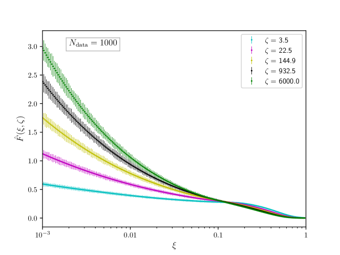
Figure 2: The pseudodata set for the observable $\hat{F}(\xi,\zeta)$, Eq. (22), used in our determination of the functions $N_{1}$ and $N_{2}$. The data points correspond to 200 points in $\xi$ logarithmically distributed in the interval $[10^{-3},\,1]$ for each of 5 different values of $\zeta$. The uncertainties are uniformly distributed between $5\%$ and $7\%$.

For ${\boldsymbol{N}}$ in Eq. (22) we have chosen the architecture $[2,10,2]$ for a total of 52 free parameters. The complexity of such a large parameter space may lead to a possible dependence of the results on the starting point of the fit in the parameter space. To avoid this problem, we performed $N_{\rm rep}=100$ replica fits of 1000 iterations each, initialising the parameters of the NN randomly in the interval $[-1,1]$ with a uniform distribution. The results will then be presented as averages over the 100 replicas with uncertainties given by the standard deviation.

Fig. 3 shows the predictions obtained after the fit, normalised to the central value of the pseudodata, plotted as a function of $\xi$ for all values of $\zeta$. The vertical error bars correspond to the pseudodata uncertainties. The agreement is evidently excellent. Indeed, the predictions overlap perfectly with the central value of the pseudodata. In addition, the uncertainty band of the predictions (plotted but not visible) is much smaller than the pseudodata uncertainties. This last observation leads to the conclusion that the final results are almost completely insensitive to the starting point of the fit in the parameter space.

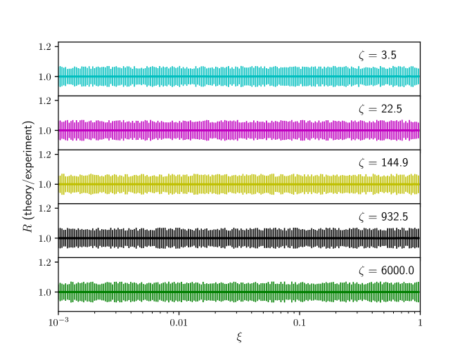
Figure 3: Ratio of predictions over data for the observable $\hat{F}(\xi,\zeta)$ for all the data included in the fit. The ratios are plotted as functions of $\xi$ for all the different values of $\zeta$.

Finally, it is interesting to compare the fitted quantities $N_{1}$ and $N_{2}$ appearing in Eq. (22) to their “truth”, i.e. the functions used to produce the pseudodata. This comparison is shown in Fig. 4. As expected, the agreement is excellent, particularly for the function $N_{2}$. The lower insets of Fig. 4 clearly show that the spread deriving from starting the fit from different points in the parameter space is generally small. This points to the fact that, despite the complexity of the parameter space, all the fits converge towards the same minimum of the $\chi^{2}$ irrespective of the starting point.

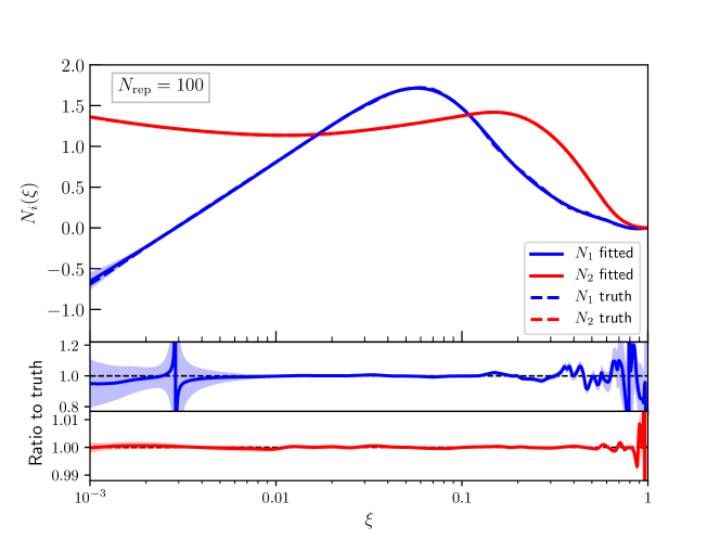
Figure 4: The central value and standard deviation of the fitted $N_{1}$ and $N_{2}$ compared to their respective “truth” taken from NNPDF31_nlo_pch_as_0118.

In conclusion, the ability of fitting functions involved in convolution integrals is a further validation of the goodness of our derivative formula in Eq. (16).

5 Performance assessment

In this section, we gauge the performance advantage of using the analytic back-propagation formula Eq. (16), detailed in Sect. 3 and used in Sect. 4, over the automatic and numerical methods as implemented in ceres-solver [1].

Numerical differentiation only relies on the knowledge of the function to be differentiated in the vicinity of the differentiation point, in a way that derivatives are computed in terms of incremental ratios. This method has the advantage that it applies straightforwardly to any function. The drawback is that it is typically slower and potentially less accurate than an analytic approach.

Automatic differentiation is instead an analytic approach that relies on dual numbers (or Jets in the language of ceres-solver). In our context, a Jet represents a parameter and its derivatives w.r.t. all other parameters in the computational graph that either precede it (in forward-mode) or succeed it (in backward-mode). Specifically, it contains a scalar value corresponding to the parameter itself and the vector of its derivatives. With a set of elementary operations, it allows for an iterative application of the derivative chain rule so that any parameter derivative could be easily computed from another connected one in the graph. Our method closely follows this procedure. However, as pointed out in Sect. 3, Eq. (16) has the advantage that the full set of derivatives is obtained in one shot iterating backwards through the NN. Conversely, standard automatic derivatives are typically computed in batches - not simultaneously - and not necessarily taking advantage of any possible iterative structure of the function being differentiated. Nonetheless, it should be pointed out that automatic differentiation is a totally general method, not specific to feed-forward NNs as our method is.

In order to compare the efficiency of the different differentiation strategies, we considered the same minimisation problem discussed in Sect. 4.1 in which a NN with a single hidden layer was fitted to pseudodata produced using a (shifted) Legendre polynomial of degree 10 as an underlying law. As in Sect. 4.1, each fit was stopped at the 1000-th iteration but the data set was extended from $N_{\rm data}=100$ to $N_{\rm data}=1000$ pseudodata points evenly distributed in the interval $[-1,1]$.

The comparison is done by recording, for all the three differentiation strategies, the fitting time as a function of the number of nodes of the hidden layer. Despite the fitting time for each differentiation strategy only depends on the number of iterations (1000 in our case), we required that only successful fits that converged towards the global minimum of the $\chi^{2}$ were considered. To this end, for every architecture, we performed 50 independent fits to the same data set with the NN initialised differently at each fit. We then selected the running time of that with the smallest $\chi^{2}$. The result of this procedure for the three differentiation strategies is shown in Fig. 5. Somewhat expectedly, the numerical differentiation (green curve) is by far the least efficient (note the logarithmic scale on the $y$ axis), being around a factor 5 slower than the automatic differentiation (red curve) and by a factor between 15 (for 22 parameters) and 50 (for 148 parameters) slower than the analytic differentiation (blue curve). More surprising is instead the difference between automatic and analytic differentiations. While the departure is smaller for relatively small numbers of parameters, it steadily increases as the number of parameters grows, with automatic differentiation being around 10 times slower than the analytic one for 148 parameters. This behaviour suggests that the iterative structure of Eq. (16) provides a performance advantage w.r.t. standard automatic differentiation as implemented in ceres-solver.

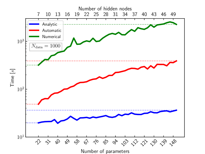
Figure 5: Comparison of the performance of the three differentiation strategies. The plot shows the minimisation time as a function of the number of parameters/nodes for fits of 1000 iterations of a single-layer NN to a Legendre polynomial of degree 10.

In order to support this hypothesis, we have increased the number of hidden layers of the NN (depth), this time limiting the comparison to automatic and analytic derivatives only. The conjecture is that deeper NNs make automatic differentiation increasingly more expensive, the reason being that the chain of derivatives to be computed is on average longer for a NN with more layers. Despite this should be the case also for the analytic back-propagation, Eq. (16), the performance worsening is expected to be milder. The reason is that the derivative w.r.t. a parameter belonging to a given layer only depends on the derivatives of the parameters in the preceding layer. Since at each iteration of a fit the derivatives w.r.t. all free parameters are used, our approach is advantageous in that a single iteration through the NN allows one to obtain them all.

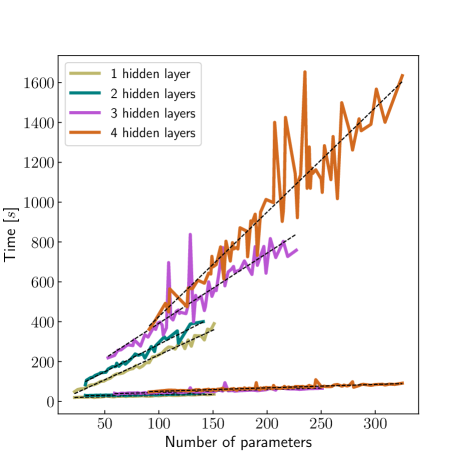
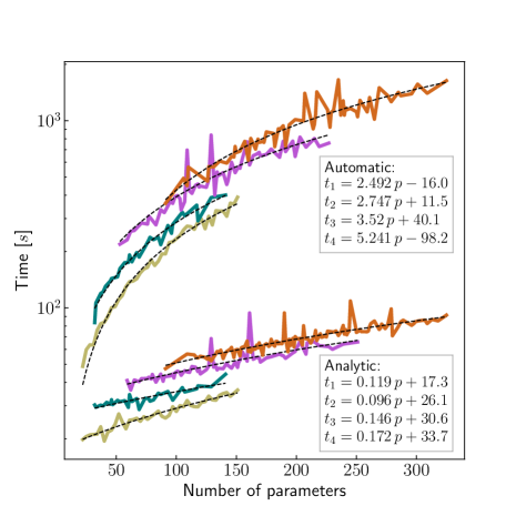
Figure 6: Performance comparison between automatic (ceres-solver) and analytic (NNAD) differentiations based on the minimisation problem discussed in Sect. 4.1. Different NN depths are also probed to highlight the differences between the two methods.

Fig. 6 clearly shows a different pattern between the analytic curves (lower part of the plot) and the automatic ones (upper part) as the depth increases. The left and right panels display the same curves in linear and logarithmic scale on the $y$ axis, respectively: the latter has the goal to make the single curves distinguishable, while the former highlights the difference in slope. To make the comparison more quantitative, we have fitted the curves with a straight line and reported slope and offset in the right panel of Fig. 6. We observe the following differences:

• In the analytic case, the performance proportionality with the number of parameters remains roughly constant across all NN depths. This is proven by the limited variation of the slopes and particularly evident in the left panel of Fig. 6 where the corresponding curves are remarkably flat.

• Conversely, in the automatic case, the slope increases significantly by increasing the NN depth. This is also evident from the left panel of Fig. 6 and the numerical values of the slopes.

From the right panel of Fig. 6, it is easier to see that both analytic and automatic curves tend to shift upwards as the NN depth is increased. This is a common feature probably because the time spent to iterate over the layers of a deeper NN is longer in both cases.

The observations concerning the performance of the different differentiation strategies seem to support our conjecture that the iterative structure of Eq. (16) is more efficient than numerical and standard automatic differentiations as implemented in ceres-solver. More specifically, our analytic derivation is accomplished through a reduced amount of computations, making it particularly efficient for large-scale problems involving deep feed-forward NNs.

6 Conclusions

In this paper, we derived a compact expression for the analytic derivatives of a feed-forward NN w.r.t. its free parameters known as back-propagation (Eq. (16)) and implemented it in the C++ NNAD code (see NNAD.git).

We presented two applications: a fit of pseudodata generated using a Legendre polynomial and a fit of functions involved in convolution integrals. These applications, implemented in the NNAD-Interface repository (see NNAD-Interface.git), prove the robustness of our analytic derivation.

We finally assessed the performance gain of using our analytic derivatives over automatic and numeric differentiation as provided by ceres-solver [1]. In order to do so, we measured the time spent to fit the “Legendre” pseudodata as a function of the number of free parameters of the NN for each of the three methods. On top of the expected performance improvement w.r.t. to numeric differentiation, we find that our analytic implementation is also significantly faster than the automatic one provided by ceres-solver. We also find that the improvement does not only trivially scale with the number of parameters, but also with the depth of the NN architecture. We interpreted this behaviour as a consequence of the exploitation of the specific recursive structure of a feed-forward NN in our analytic back-propagation formula. We thus conclude that NNAD is particularly suited for large-scale problems.

We would finally like to stress that we are aware of the plethora of available minimisers dedicated to problems involving neural networks, such as Tensorflow [12], PyTorch [13], and Keras [14]. However, a typical feature of these tools is that their mainstream user interface is written in python. Therefore, a direct comparison of our back-propagation formula to the differentiation strategies of these codes, would require a python implementation of NNAD. We do plan to carry out such an implementation, along with comparisons to the main available tools, in a future publication.

Appendix A General overview of the NNAD code

In this appendix we discuss the main functionalities of the NNAD implementation of a feed-forward NN and its analytic derivatives. An example code can be found in the public distribution of the NNAD code under the name tests/TestDerivatives.cc. The purpose of that code is to build a NN, compute the NN itself and all its derivatives at some particular point, and finally compare the results to a fully numerical calculation.

The first step to take is the definition of the architecture of the NN in terms of a std::vector of int’s, for example:

  // Define architecture
  const std::vector<int> arch{3, 5, 5, 3};

This defines the architecture $[3,\,5,\,5,\,3]$ with three input nodes, two fully-connected hidden layers with five nodes each, and three output nodes. The next step is to build the NN itself and this is easily done as follows:

  // Initialise NN
  const nnad::FeedForwardNN<double> nn{arch, 0, true};

The NN is an object of the template namespaced class FeedForwardNN that takes as (mandatory) inputs the architecture and a random seed (0 in this case) required to randomly initialise weights and biases between zero and one. There are further optional inputs. The first is a switch to turn on or off the report of the NN features. This parameter is off by default but it is turned on in the example above. As a further input, the user can specify the functional form of the activation function $\phi$ (that is used for all non-input nodes) and its derivative $\phi^{\prime}$. It is responsibility of the user to make sure that activation function and its derivative correctly match. Both these inputs should be passed as std::function’s taking a double as an input and returning a double. The default for these parameters is the sigmoid function and its derivative:

$$\phi(x)=\frac{1}{1+e^{-x}}\,,\qquad\phi^{\prime}(x)=\phi(x)\left[1-\phi(x)\right]\,.$$ (26)

The final optional input is whether the output nodes should use the same activation function of the hidden nodes or if their activation function should be linear. The code uses linear activation functions as a default for the output nodes.

Once the NN object has been built, one needs to define an input that has to be a std::vector of double’s with as many elements as input nodes: three, in this case. For example:

  // Input vector
  std::vector<double> x{0.1, 2.3, 4.5};

There are two main methods to evaluate the NN at x. The first is:

  // Get NN at x
  std::vector<double> nnx = nn.Evaluate(x);

that returns a std::vector of double’s with as many elements as output nodes (three, in this case) corresponding to the NN values. In order to also access the derivatives, one can call:

  // Get NN and its derivatives at x
  std::vector<double> dnnx = nn.Derive(x);

Also this function returns a std::vector of double’s but with as many elements as output nodes plus the number of parameters times the number output nodes. In fact, the function Derive, not only returns the derivatives, but also the values of the NN itself that are placed in the first (three, in this case) entries of the vector dnnx.

The class FeedForwardNN provides more methods to handle its objects. A more detailed documentation can be found in the online repository.

References

- [1] S. Agarwal, K. Mierle, Others, Ceres solver, http://ceres-solver.org.
- [2] S. Forte, L. Garrido, J. I. Latorre, A. Piccione, Neural network parametrization of deep inelastic structure functions, JHEP 05 (2002) 062. arXiv:hep-ph/0204232, doi:10.1088/1126-6708/2002/05/062.
- [3] K. Kumericki, D. Mueller, A. Schafer, Neural network generated parametrizations of deeply virtual Compton form factors, JHEP 07 (2011) 073. arXiv:1106.2808, doi:10.1007/JHEP07(2011)073.
- [4] R. D. Ball, et al., Parton distributions from high-precision collider data, Eur. Phys. J. C 77 (10) (2017) 663. arXiv:1706.00428, doi:10.1140/epjc/s10052-017-5199-5.
- [5] A. Auger, N. Hansen, A restart cma evolution strategy with increasing population size, in: 2005 IEEE Congress on Evolutionary Computation, Vol. 2, 2005, pp. 1769–1776 Vol. 2.
- [6] H. P. Gavin, The levenberg-marquardt method for nonlinear least squares curve-fitting problems c ©, 2013.
- [7] V. Bertone, S. Carrazza, N. P. Hartland, APFELgrid: a high performance tool for parton density determinations, Comput. Phys. Commun. 212 (2017) 205–209. arXiv:1605.02070, doi:10.1016/j.cpc.2016.10.006.
- [8] R. Abdul Khalek, J. J. Ethier, J. Rojo, Nuclear parton distributions from lepton-nucleus scattering and the impact of an electron-ion collider, Eur. Phys. J. C 79 (6) (2019) 471. arXiv:1904.00018, doi:10.1140/epjc/s10052-019-6983-1.
- [9] V. Bertone, S. Carrazza, N. P. Hartland, E. R. Nocera, J. Rojo, A determination of the fragmentation functions of pions, kaons, and protons with faithful uncertainties, Eur. Phys. J. C 77 (8) (2017) 516. arXiv:1706.07049, doi:10.1140/epjc/s10052-017-5088-y.
- [10] V. Bertone, S. Carrazza, J. Rojo, APFEL: A PDF Evolution Library with QED corrections, Comput. Phys. Commun. 185 (2014) 1647–1668. arXiv:1310.1394, doi:10.1016/j.cpc.2014.03.007.
- [11] A. Buckley, J. Ferrando, S. Lloyd, K. Nordström, B. Page, M. Rüfenacht, M. Schönherr, G. Watt, LHAPDF6: parton density access in the LHC precision era, Eur. Phys. J. C 75 (2015) 132. arXiv:1412.7420, doi:10.1140/epjc/s10052-015-3318-8.
-
[12]
TensorFlow: Large-scale machine learning on
heterogeneous systems, software available from tensorflow.org (2015).
URL http://tensorflow.org/ -
[13]
Pytorch:
An imperative style, high-performance deep learning library, in: Advances in
Neural Information Processing Systems 32, Curran Associates, Inc., 2019, pp.
8024–8035.
URL http://papers.neurips.cc/paper/9015-pytorch-an-imperative-style-high-performance-deep-learning-library.pdf - [14] F. Chollet, et al., Keras, https://keras.io (2015).
- [15] V. Bertone, et al., xFitter 2.0.0: An Open Source QCD Fit Framework, PoS DIS2017 (2018) 203. arXiv:1709.01151, doi:10.22323/1.297.0203.