Plane-Activated Mapped Microstructure

Abstract

Querying and interacting with models of massive material micro-structure requires localized on-demand generation of the micro-structure since the full-scale storing and retrieving is cost prohibitive. When the micro-structure is efficiently represented as the image of a canonical structure under a non-linear space deformation to allow it to conform to curved shape, the additional challenge is to relate the query of the mapped micro-structure back to its canonical structure.

This paper presents an efficient algorithm to pull back a mapped micro-structure to a partition of the canonical domain structure into boxes and only activates boxes whose image is likely intersected by a plane. The active boxes are organized into a forest whose trees are traversed depth first to generate mapped micro-structure only of the active boxes. The traversal supports, for example, 3D print slice generation in additive manufacturing.

jyoungquist@ufl.eduJeremy Youngquist

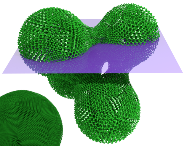
Figure 1: Mapped micro-structure and slice plane. The map is piecewise cubic. Left foreground: High-resolution micro-structure.

1 Introduction

State-of-the-art 3D printers are capable of printing structure at the micrometer [1] and even nanometer [2] scale. Additive manufacturing therefore, in principle, allows designs that spatially vary and optimize the material properties of objects via their micro-structure [3, 4, 5, 6]. However, a one meter cube with micrometer structures challenges existing storage capacities and deliberate access. The natural response, to generate the micro-structure on demand, is not without its own problems. New fast printers are able to print fine-scale micro-structures over regions up to one million times larger than the feature size [7, 8]. Therefore micro-structure generation must be very fast and activated with keen focus on the query.

An additional challenge is to conform to curved shapes without breaking the structure at a boundary, compromising its structural integrity. One solution is to generate micro-structure as the mapped image of a canonical structure, i.e. under a non-linear space deforming map. This kind of 3D morphing allows the micro-structure to fill, for example, a curved tetrahedral partition of a macro-shape as in Figure 1 adapted from [9, 10]. However, any query now has to be pulled back from the mapped image to the canonical domain micro-structure.

This paper presents an efficient algorithm to pull back and so activate mapped micro-structure intersected by a plane; and so enable slice generation of massive mapped micro-structures for 3D printing. The approach generates micro-structure only in a close neighborhood of the plane in $\mathbb{R}^{3}$, and is agnostic as to the shape of the canonical structure and its partition into local pre-images. We will illustrate the approach by hex-paving the tetrahedral domain of a piecewise total degree 3 map in Bernstein-Bézier form.

\begin{overpic}[scale={0.48}]{fig_1_v8_smaller.png} \put(38.0,26.0){\huge$\displaystyle\mathbf{g}$} \end{overpic}

Figure 2: Mapping $\mathbf{g}(\footnotesize{\Box}_{\beta})$. Left: Tetrahedron $\Delta$ with box partition. Middle: Curved $\mathbf{g}(\Delta)$ with overlapping cuboids. Note that the pre-image of the slicing plane is a curved surface. Right: The full set $\mathbf{g}_{i}(\Delta)$ with the exterior face of the specific $\mathbf{g}(\Delta)$ is marked yellow.

2 Related Work

2.1 Slicing

Surface slicing algorithms take as input a triangulated surface and return a set of oriented boundary curves representing the intersection of that surface with a set of slice planes. These boundary curves are used to generate infill and machine instructions for the printer.

Leveraging massively parallel architecture, GPU-based methods can provide up to a 30x speedup over similar CPU-based algorithms [11, 12, 13] and out-of-core slicing algorithms reduce the memory burden for larger meshes by keeping the mesh on the hard drive rather than the memory of the computer[14, 15]. However, these out-of-core methods have quadratic complexity in the number of triangles. An optimal slicing algorithm [16] can be designed to have complexity linear in the number of triangles, the number of slice planes, and the number of triangle-plane intersections, provided the slices have uniform thickness. However, this algorithm takes as input the entire mesh, and thus is ruled out for procedurally generated or massive micro-structures.

Generating micro-structure on-demand has been explored [17]. However the materials are defined directly as the voxelized signed-distance map in the physical space $\mathbb{R}^{3}$ rather than as a parametric map of some simpler pre-image. It therefore does not conform to curved shapes and does not follow the spirit of state-of-the-art modelling and analysis tools, such as isogeometric analysis. Isogeometric analysis uses parametric maps, splines or Bézier functions. A second drawback of the approach in [17] is that each slice has to be generated in its entirety and is therefore limited in size and fineness of the micro-structure.

In this paper, we address both challenges, introducing a streaming architecture capable of printing micro-structures defined on parametric spaces with slices of massive size.

2.2 Procedural Microstructure

Procedural micro-structures are defined by a function $p:\mathbb{R}^{3}\rightarrow\{0,1\}$ identifying points belonging to the micro-structure [18, 19, 20]. In order to be computationally efficient, $p$ must have $\mathcal{O}({1})$ time and space complexity independent of the evaluation point. Furthermore, if the structure is to be printed, $p$ must define support structures (if required) and satisfy overhang criteria [20].

Many classes of sufficiently fine-scale micro-structures behave as if they were a continuum, with the continuum behavior increasing in accuracy as the micro-structure grows finer [21, 22, 23]. This allows for specification of functionally graded material properties of procedural models while still treating them with continuum analysis. This has been successfully integrated into analysis tools to optimize microstructure to conform to a spatially varying compliance matrix [3, 4, 5, 6].

However, for such micro-structure to be used with state-of-the-art isogeometric analysis tools, they should be defined in the parametric space of the isogeometric elements. Defining micro-structure in the parametric space of a free-form deformation is also necessary to leverage the standard tools of computer-aided geometric design and conform the micro-structure to curved objects [9, 24, 25]. Although micro-structure defined by $p$ directly in $\mathbb{R}^{3}$ is mostly straightforward to locally generate on-demand [17], for $p$ mapped by a macro-scale parametric function it is necessary to find the pre-image of every voxel in $\mathbb{R}^{3}$ – and isogeometric elements do not in general have analytic inverses.

The algorithm presented in the following addresses these challenges by generating on-demand micro-structure defined on parametric elements.

3 Preliminaries and Definitions

We consider a typical 3D deformation map [26] in total degree $m$ Bernstein-Bézier form (BB-form), see e.g. [27]:

$$\mathbf{g} :\Delta\subset\mathbb{R}^{3}\rightarrow\mathbb{R}^{3}\qquad\sum\alpha_{i}=m,\ \alpha_{i}\geq 0,$$

$$\mathbf{g}(\mathbf{u}) :=\sum_{\alpha}\mathbf{g}_{\alpha}B_{\alpha}(\mathbf{u}),\quad B_{\alpha}(\mathbf{u}):=\frac{m!}{\alpha_{0}!\alpha_{1}!\alpha_{2}!\alpha_{3}!}\prod_{i=0}^{3}\mathbf{u}^{\alpha_{i}}_{i},$$ (1)

Since injectivity is mandatory when generating micro-structure and large deformations unduly stretch or squeeze, we may assume that $\mathbf{g}$ satisfies $0<\det{\nabla\mathbf{g}}<M$ for some constant $M$. That is the Jacobian determinant is nonzero and bounded. Assuming, without loss of generality, a slicing plane of constant $z=z_{0}$ and denoting the z-coordinate of $\mathbf{g}$ by $\mathbf{g}^{z}$, the Pre-image Theorem then certifies the pre-image $\{\mathbf{u}:\mathbf{g}^{z}(\mathbf{u})=z_{0}\}$ is bivariate without jumps, and with holes only due to the boundaries of $\Delta$.

3.1 Safe pre-image traversal

The key to efficiently activating polyhedral sub-regions $\footnotesize{\Box}_{\beta}$ of $\Delta$ in order to fill it with micro-structure is to determine whether $\mathbf{g}(\footnotesize{\Box}_{\beta})$ intersects the slice plane. For the vertices $\mathbf{v}_{i}$ of $\footnotesize{\Box}_{\beta}$, let $\footnotesize{\Diamond}_{\beta}$ be a polyhedral sub-region of $\mathbb{R}^{3}$ delineated by $\mathbf{g}(\mathbf{v}_{i})$.We will test against an enlargement of $\footnotesize{\Diamond}_{\beta}$ whose intersection with the slicing plane then identifies $\footnotesize{\Box}_{\beta}$ with $\mathbf{g}(\footnotesize{\Box}_{\beta})$ that can intersect the plane.

The enlargement depends on how much $\mathbf{g}(\Delta)$ differs from the linear function $\ell:\Delta\to\mathbb{R}^{3}$ that interpolates the mapped vertices $\mathbf{g}(\mathbf{v}_{i})=\mathbf{g}_{3\mathbf{e}_{k}}$ that form a simplex $S$. Generalizing an estimate for the bivariate total degree case [28], we obtain for the trivariate case

$$\sup_{\mathbf{u}\in\Delta}\|\mathbf{g}-\ell\|\leq\frac{1}{8}\sum_{i,j\in\{1,2,3\}}l_{i}l_{j}\sup_{\mathbf{u}\in\Delta}\|\partial_{\mathbf{u}_{i}\mathbf{u}_{j}}\mathbf{g}\|$$ (2)

where $l_{i}$ is initially the unit length of the domain with respect to variable $\mathbf{u}_{i}$. Here the mixed partials $i\neq j$ are counted twice for a total of 9 terms of which only 6 are different.

For $\mathbf{g}$ of degree 3, $\partial_{\mathbf{u}_{i}\mathbf{u}_{j}}\mathbf{g}$ is linear, and each of the six expressions, attains its maximum at one of its four vertices. As is well-known for polynomials in BB-form [29], the values of $\partial_{\mathbf{u}_{i}\mathbf{u}_{j}}\mathbf{g}$ at each of its four vertices are $6$ times the second differences at the vertex. Equivalently, we compute for $k\in\{1,2,3,4\}$ the six second differences of the BB-coefficients

$$\mathbf{d}_{ijk}:=\mathbf{g}_{3\mathbf{e}_{k}}-\mathbf{g}_{2\mathbf{e}_{k}+\mathbf{e}_{i}}-\mathbf{g}_{2\mathbf{e}_{k}+\mathbf{e}_{j}}+\mathbf{g}_{\mathbf{e}_{k}+\mathbf{e}_{i}+\mathbf{e}_{j}},\quad\text{ for }i\neq k\neq j$$ (3)

Then $\mathbf{g}(\Delta)$ is enclosed by offsetting $S$ in $x$ by

$$\mu^{x}:=\frac{6}{8}\sum_{i,j\in\{1,2,3\}}l_{i}l_{j}\max_{k}|\mathbf{d}^{x}_{ijk}|$$ (4)

where $\mathbf{d}^{x}_{ijk}$ is the $x$-coordinate of $\mathbf{d}_{ijk}$, and offset likewise in $y$ and $z$.

If we split each edge of the domain $\Delta$ into $n=2^{\nu}$ pieces then $l_{i}l_{j}$ becomes $4^{-\nu}$ times the initial unit edge length and for polyhedral $\footnotesize{\Box}_{\beta}$ with side-lengths $l_{i}<2^{-\nu}$, it suffices to test $\footnotesize{\Diamond}_{\beta}$ offset by $\mu/4^{\nu}$. The algorithm intersects the edges of $\footnotesize{\Diamond}_{\beta}$ with the planar slice using a tolerance of $\mu/4^{\nu}$.

While tighter bounds of the images of the $\footnotesize{\Box}_{\beta}$ can be obtained, by explicit subdivision of $\mathbf{g}$ or by sleves [30], we expect the number of sub-regions to be very large so that $4^{-\nu}$ is the dominant factor.

3.2 Box paving

To emphasize the generality of the approach, we choose the sub-regions $\footnotesize{\Box}_{\beta}$ of $\Delta$ to be deformed cubes, called boxes. Then the $\footnotesize{\Diamond}_{\beta}\in\mathbb{R}^{3}$ are called (image) $cuboids$. Crucially, the boxes will conform to and fill the domain $\Delta$ without overlap. So we do not need to be concerned about partially filled or clipped boxes as occur when superimposing a uniform grid on $\Delta$. By contrast, the cuboids $\footnotesize{\Diamond}_{\beta}$ typically overlap when offset by $\mu$, but this is of little consequence since they only serve to identify their domain boxes.

\begin{overpic}[scale={0.35},trim=40.15pt 60.22499pt 200.74998pt 70.2625pt,clip,width=346.89731pt]{fig_14_smaller.pdf} \put(50.0,38.0){\footnotesize{ijk}} \put(35.0,40.0){\footnotesize{120}} \put(23.0,40.0){\footnotesize{110}} \put(13.0,40.0){\footnotesize{100}} \put(12.0,15.0){\footnotesize{000}} \put(25.0,15.0){\footnotesize{010}} \put(37.0,15.0){\footnotesize{020}} \put(47.0,15.0){\footnotesize{030}} \put(12.0,80.0){\footnotesize{300}} \end{overpic}

Figure 3: Paving of a tetrahedral $\Delta$ by boxes with resolution $n=2^{\nu}$.

Figure 3 illustrates the approach by paving a tetrahedron so that layer $i$ has $n-i$ rows and row $j$ of the layer $i$ has $n-i-j$ boxes. Each box can then be identified by the ID triple of integers $(layer,row,col)$. At the apex, the paving degenerates into a tetrahedron but this is not a problem since boxes are only used to identify neighbors in $\Delta$. Each box has up to 12 neighbors in this partition.

While, at first, it may seem odd to pave a tetrahedron with boxes, we note that a partition into small tetrahedra requires more complex indexing to visit neighbors.

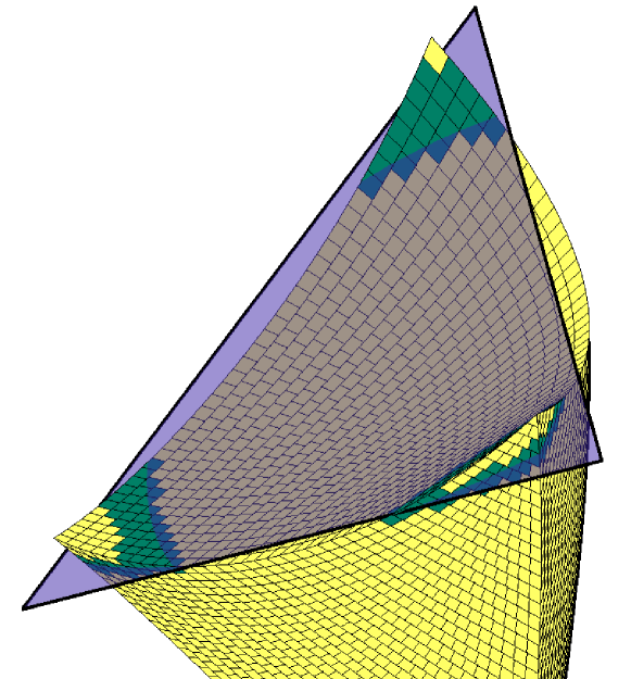
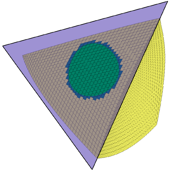
Figure 4: Top: A single slice with multiple components due to intersecting edges. Bottom: Closed loop intersection on a face (does not intersect any edges).

4 Algorithm

Given a set $G$ of maps $\mathbf{g}_{i}$, a partition of the shared domain $\Delta$ into boxes $\footnotesize{\Box}_{\beta}$, and a set of planes $p_{j}\in P$, the goal is to efficiently traverse, for each $\mathbf{g}_{i}$ and $p_{j}$, all boxes $\footnotesize{\Box}_{\beta}$ such that $\mathbf{g}_{i}(\footnotesize{\Box}_{\beta})\cap p_{j}\not=\emptyset$. The key to efficiency is to activate (generate or retrieve from temporary storage) only those boxes whose image can overlap the current slice plane $p_{j}$. Then depth-first traversal minimizes generation and temporary storage of micro-structure.

4.1 Reduction to a single map and plane

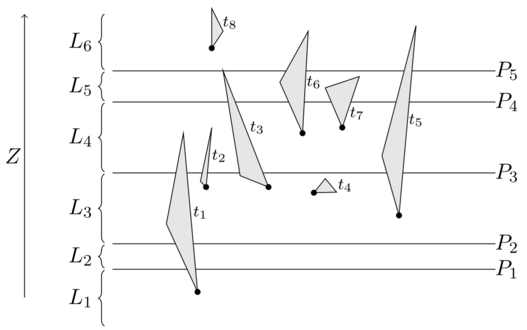
Figure 11: Illustration of the tetrahedral list algorithm, from [16]. Each $L[i]$ contains the tetrahedra whose lowest value is between $P[i-1]$ and $P[i]$.

After sorting the $\mathbf{g}_{j}$ into range list $L$ (see Figure 11) the outer loop of the algorithm performs an optimized plane sweep through all $\mathbf{g}_{j}$ that possibly intersect plane $p_{i}$. Appendix A lists the simple main Algorithm 1 where highlighted routines perform the intersection of one map-plane pair discussed below and $L[i]$ in Algorithm 2 is the set of $\mathbf{g}_{j}$ which become active at plane $P[i]$. The minimal $z$ coordinate of the Bézier coefficients of $\mathbf{g}_{j}$, $\mathbf{g}^{z}_{j}$ must lie between the $z$ coordinates of $p_{i}$ and $p_{i+1}$: $P[i]\leq\mathbf{g}^{z}_{j}<P[i+1]$. The convex hull property of the BB-form then guarantees that no $\mathbf{g}_{j}$ outside the list is intersected by the slicing plane. Building the list, Algorithm 2, generalizes [16] to maps $\mathbf{g}_{j}$; this can be optimized if the $\mathbf{g}_{j}$ are already sorted or the planes have uniform thickness.

In the following we illustrate the algorithm with a single polynomial map $\mathbf{g}$ of total degree 3 in Bernstein-Bezier form, $\Delta$ a tetrahedron, and a single plane $p$ with normal $(0,0,1)$.

4.2 Components of one map-plane intersection

Due to the curvature of $\mathbf{g}$, the intersection $\mathbf{g}(\Delta)\cap p$ can have multiple disconnected components (see Figure 4). If we consider each box as a node connected via an edge to its neighboring boxes, the algorithm traces out a tree for each component starting a depth-first search from a box known to straddle the plane. Since we can assume that the pre-images of slices through $\mathbf{g}(\Delta)$ are surfaces, disconnected components occur only by slicing through the boundary. We find all disconnected components by testing the cuboids of the edges of $S$ (Algorithm 4), and then test the faces of $S$ for closed loops. A closed loop intersection can occur only if a face’s surface $\mathbf{g}^{s}(t_{1},t_{2})$, $i=0,1,2,3$ has a normal $\mathbf{n}^{s}$ orthogonal to the slicing plane [31]. If the BB-coefficients of $\det(\mathbf{n},\partial_{t_{1}}\mathbf{g}^{s},\partial_{t_{2}}\mathbf{g}^{s})$ are of one sign there is no loop. If the criterion fails to rule out an intersection, we find any by traversing and testing all cuboids of the face.

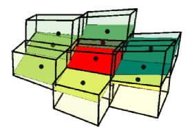
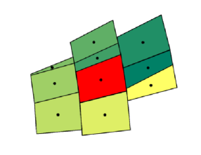
Figure 5: Planar cut through active cuboids $\footnotesize{\Diamond}_{\beta}$. Top: 3D view, bottom: intersection with slice plane only. The current $\footnotesize{\Diamond}_{\beta}$ is red, the neighbors are sorted counterclockwise by their centers $\bullet$ and colored in traversal order from dark green to yellow.

4.3 Traversal of one map-plane pair

For each new tetrahedron-plane pair, the algorithm initializes (Algorithm 3 in Appendix B) and starts with a box found by Algorithm 4. A stack, $toRevisit$, and a hashmap, $visitedBoxes$, store the box IDs of cuboid-plane intersections.

With each iterator increment, we are either at the first and only box of an isolated component and jump to another component by Algorithm 8; or we activate an intersecting neighbor (Algorithm 6).

4.4 Iteration

To find the next box (Algorithm 6) we first find the set of neighboring boxes whose cuboids intersect the plane and, associating each box with the center of its cuboid’s intersection with the plane (see $\bullet$ in Figure 5), sort the centers clockwise about the center of the current box with respect to the previous box. After removing the boxes we have already visited, we proceed to the next box in the list, setting $currBox$ to this box ID and adding the ID to both $toRevisit$ and $visitedBoxes$. Once all eligible neighbors have been visited, Figure 6, we backtrack (Algorithm 7) by popping box IDs off the $toRevisit$ stack until an eligible box is found.

If the $toRevisit$ stack is empty, we continue with another connected component (Algorithm 8), restarting the iteration with a box ID in the list of eligible boundary boxes until empty. If there are no more boundary boxes, then the intersection is complete and $isValid$ is set to false.

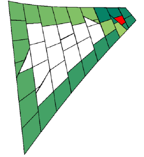
Figure 6: A red leaf node of the traversal tree: all neighbors have been visited, but the slice is not yet fully covered and requires backtracking. The completed traversal tree is shown in Figure 7.

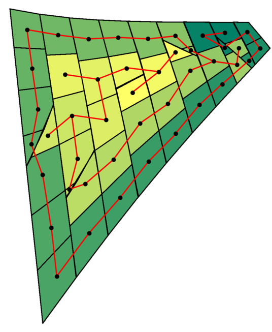
Figure 7: The path traced out by the algorithm is a tree.

5 Complexity Analysis

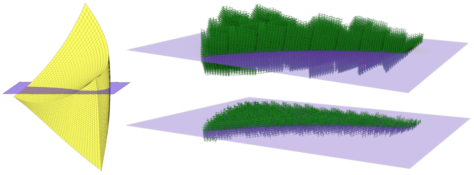
Figure 8: As the number of boxes increases, less micro-structure (bottom vs. top) needs to be generated.

Here we analyze the complexity of activating a single map-plane pair.

Letting $n$ be the number of boxes along one axis of $\Delta$ there are $\mathcal{O}({n^{2}})$ boxes on each face of the tetrahedron. Because the pre-image of the slice plane is a bivariate manifold, there are $k{n^{2}}$ $\footnotesize{\Diamond}_{\beta}$ straddling the slice, where $k$ depends on the tightness of the estimate $\mu^{x}$ of (4) since the cuboids will overlap.

Each push or pop on the $toRevisit$ stack, and each get or put on the $alreadyVisited$ hashmap has unit cost.

5.1 Initialization

The complexity of initializing the iterator is bounded by the time it takes to build the list of cuboids that straddle the boundary. It takes just $\mathcal{O}({n})$ to iterate across each edge but $\mathcal{O}({n^{2}})$ to iterate over a face.

5.2 Iteration

Construct a graph by treating each intersecting cuboid as a node connected to its neighboring cuboids by edges. Since there are $\mathcal{O}({n^{2}})$ cuboids in the intersection, this graph has $\mathcal{O}({n^{2}})$ vertices. The algorithm traces out a spanning forest of this graph, which is linear in the number of vertices. Thus the iteration complexity is $\mathcal{O}({n^{2}})$.

5.3 Space Complexity

The $\mathcal{O}({n^{2}})$ triple integer lists of IDs, $toRevisit$ and $visitedBoxes$, are the only data structures that grow in size proportional to $n^{2}$. They are lightweight and reset for each tetrahedron and slice plane.

6 Generating Micro-structure

Since our focus is on accessing the micro-structure, Section 4 intentionally did not discuss the actual slicing of the micro-structure with the mapped box for streamed printing, which depends on the details of the printing setup and micro-structure definition.

For a fixed micro-structure, increasing the number $n$ of boxes decreases the box size and hence the amount $g(n)$ of micro-structure to be generated per box. Thus the total complexity for iterating through the slice and generating the micro-structure is $\mathcal{O}({n^{2}g(n)+n^{2}})$. Since $g(n)$ is inversely proportional to $n$, note that $\mathcal{O}({n^{2}g(n)})$ can decrease with $n$ due to reduced thickness, see Figure 8.

Trading time and space complexity, we can re-generate micro-structure repeatedly for each slice, or store it under its box ID in a list of active boxes as the plane moves.

Examples

The practicality of the algorithm is illustrated by slicing an extremely fine micro-structure on a mesh with 738 maps, 235 of which intersect the slice plane. Figure 9 shows the slices of the cuboids colored for traversal per $\mathbf{g}_{i}$ from dark to light.

Figure 10 shows the micro-structure generated on the mesh.

Table 1 lists run times for the generation of boxes, not including micro-structure generation or slicing.

n	Time(s)	Boxes in Intersection	Total Boxes in Tetrahedron	Intersect/Total
4	1.797e-4	7	20	35.00%
8	6.368e-4	22	120	18.33%
16	2.729e-3	79	816	9.681%
32	1.410e-2	312	5984	5.214%
64	0.1037	1,256	45,760	2.745%
128	1.462	4,914	357,760	1.374%
256	21.59	18,826	2,829,056	0.6655%
512	405.1	76,793	22,500,864	0.3413%

Table 1: Run times and number of boxes $\footnotesize{\Box}_{\beta}$ in the intersection vs number in the entire $\Delta$.

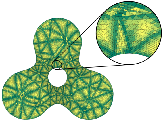
Figure 9: A slice through the mapped micro-structure of Figure 1. Each tile records one of 24,789 intersections between a cuboid and the slice plane. The colors represent the ordering of boxes within each map.

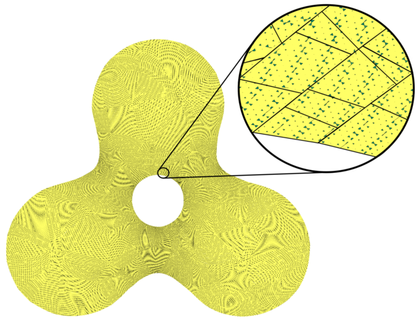
Figure 10: Slice through the mapped micro-structure of Figure 1. The enlargement reveals the micro-structure and cuboids.

7 Conclusion

This paper proposed and implemented an algorithm for selectively generating mapped micro-structure only near a plane of interest. The algorithm partitions parametric space into boxes and uses their neighborhood relations to generate only micro-structure contained in those boxes whose images intersect the plane. The algorithm has optimal asymptotic complexity.

We applied the algorithm to the slicing problem for additive manufacturing, demonstrating that our algorithm is capable of generating large slices of extremely fine-scale micro-structure. The implementation can easily be applied to hexahedra $\Delta$ in place of tetrahedra.

Appendix A: Pseudocode: Slicing Multiple $\Delta_{i}$

input : $n,T,k,P,\mathcal{G}$

$L[1,\cdots,k+1]\leftarrow$ buildTetrahedronList$(n,T,k,P)$

$A\leftarrow\{\}$ set of active tetrahedra

for $i\in{1,\cdots,k}$ do

       $A\leftarrow A\cup L[i]$

       for $tet\in A$ do

             if $tet.z_{max}<P[i]$ then

                   $A\leftarrow A\setminus{tet}$

                  

            else

                   Iterator-Initialize$(tet,P[i])$

                   while $\textsc{Iterator}-isValid$ do

                         $M\leftarrow tet.\mathbf{g}(\mathcal{G}(\textsc{Iterator-}currBox))$

                         SliceAndPrint$(M,P[i])$

                         Iterator-Increment$()$

                        

                   end while

                  

             end if

            

       end for

      

end for

return

Algorithm 1 Repeated Slicing Loop

input : $n,T,k,P$

output : $L$

$L[1,\cdots,k+1]\leftarrow\{\}$

for each $tet\in T$ do

       $i\leftarrow$ min $i$ such that $P[i]\geq tet.z_{min}$

       $L[i]\leftarrow L[i]\cup{tet}$

      

end for

return $L$

Algorithm 2 BuildTetrahedronList

Appendix B: Pseudocode: Single Map-Plane Micro-structure Activation

input : $tet,plane,\mathcal{G}$

Iterator-Initialize$(tet,plane)$

while $\textsc{Iterator}-isValid$ do

       $M\leftarrow tet.\mathbf{g}(\mathcal{G}(\textsc{Iterator-}currBox))$

       SliceAndPrint$(M,plane)$

       Iterator-Increment$()$

      

end while

return

Algorithm 3 Single Map-Plane loop

input : $tet$

$boundBoxes\leftarrow\{\}$

for each box on an edge of $tet$ do

       if $tet.\mathbf{g}($box$)$ intersects $P$ then

             $boundBoxes\leftarrow boundBoxes\cup box$

            

       end if

      

end for

for each face $F$ of $tet$ do

       if $F.N(u,v)$ is parallel to $P.normal$ for any $u,v$ then

             for each box on $F$ do

                   if $tet.\mathbf{g}($box$)$ intersects $P$ then

                         $boundBoxes\leftarrow boundBoxes\cup box$

                        

                   end if

                  

             end for

            

       end if

      

end for

return $boundaryBoxes$

Algorithm 4 Iterator-FindBoundaryBoxes

$candidates=intersectingNeighbors(currBox,T,P)$

if $candidates$ is not empty then

       FindNextBox() ;

        // Typical case

      

else

       restartOnBoundaryBox() ;

        // Only one box in component

      

end if

return

Algorithm 5 Iterator-Increment

$candidates\leftarrow intersectingNeighbors(currBox,T,P)$

$sortCCW(candidates,currBox,prevBox)$

$removeVisitedBoxes(candidates,visitedBoxes)$

if $candidates$ is not empty then

       $prevBox=currBox$

       $currBox=candidates[0]$

       $visitedBoxes.insert(currBox)$

       $toRevisit.push(currBox)$

      

else

       WalkBack() ;

        // At a leaf box

      

end if

return

Algorithm 6 Iterator-FindNextBox

if $toRevisit$ is not empty then

       while $toRevisit.top()==currBox$ do

             $toRevisit.pop()$

            

       end while

      $prevBox=currBox$

       $currBox=toRevisit.top()$

       $toRevisit.pop()$

       $visitedBoxes.insert(currBox)$

       $toRevisit.push(currBox)$

       findNextBox()

      

else

       restartOnBoundaryBox()

      

end if

return

Algorithm 7 Iterator-WalkBack

$removeVisited(boundaryBoxes,visited)$

if $boundaryBoxes$ is not empty then

       $prevBox=null$

       $currBox=boundaryBoxes[0]$

       $visitedBoxes.insert(currBox)$

       $toRevisit.push(currBox)$

      

else

       $isValid=false$

      

end if

return

Algorithm 8 Iterator-RestartOnBoundary

input : $tet,plane$

$isValid\leftarrow true$

$toRevisit\leftarrow\emptyset$

$visitedBoxes\leftarrow\emptyset$

$boundaryBoxes\leftarrow\textsc{findBoundaryBoxes}(tet)$

$prevBox\leftarrow null$

$currBox\leftarrow boundaryBoxes[0]$

$T\leftarrow tet$

$P\leftarrow plane$

return

Algorithm 9 Iterator-Initialize

References

- Fogel et al. [2018] Fogel, O, Winter, S, Benjamin, E, Krylov, S, Kotler, Z, Zalevsky, Z. 3d printing of functional metallic microstructures and its implementation in electrothermal actuators. Additive Manufacturing 2018;21:307 – 311. URL: http://www.sciencedirect.com/science/article/pii/S2214860418300861. doi:https://doi.org/10.1016/j.addma.2018.03.018.
- Vyatskikh et al. [2018] Vyatskikh, A, Delalande, S, Kudo, A, Zhang, X, Prtela, C, Greer, J. Additive manufacturing of 3d nano-architected metals. Nature Communications 2018;URL: https://doi.org/10.1038/s41467-018-03071-9. doi:10.1038/s41467-018-03071-9.
- Wang et al. [2018] Wang, Y, Zhang, L, Daynes, S, Zhang, H, Feih, S, Wang, MY. Design of graded lattice structure with optimized mesostructures for additive manufacturing. Materials & Design 2018;142:114 – 123. URL: http://www.sciencedirect.com/science/article/pii/S026412751830011X. doi:https://doi.org/10.1016/j.matdes.2018.01.011.
- Bickel et al. [2010] Bickel, B, Bächer, M, Otaduy, MA, Lee, HR, Pfister, H, Gross, M, et al. Design and fabrication of materials with desired deformation behavior. ACM Trans Graph 2010;29(4). URL: https://doi.org/10.1145/1778765.1778800. doi:10.1145/1778765.1778800.
- Schumacher et al. [2015] Schumacher, C, Bickel, B, Rys, J, Marschner, S, Daraio, C, Gross, M. Microstructures to control elasticity in 3d printing. ACM Trans Graph 2015;34(4). URL: https://doi.org/10.1145/2766926. doi:10.1145/2766926.
- Panetta et al. [2015] Panetta, J, Zhou, Q, Malomo, L, Pietroni, N, Cignoni, P, Zorin, D. Elastic textures for additive fabrication. ACM Trans Graph 2015;34(4). URL: https://doi.org/10.1145/2766937. doi:10.1145/2766937.
- Saha et al. [2019] Saha, SK, Wang, D, Nguyen, VH, Chang, Y, Oakdale, JS, Chen, SC. Scalable submicrometer additive manufacturing. Science 2019;366(6461):105–109. URL: https://science.sciencemag.org/content/366/6461/105. doi:10.1126/science.aax8760. arXiv:https://science.sciencemag.org/content/366/6461/105.full.pdf.
- Jonušauskas et al. [2019] Jonušauskas, L, Gailevičius, D, Rekštytė, S, Baldacchini, T, Juodkazis, S, Malinauskas, M. Mesoscale laser 3d printing. Opt Express 2019;27(11):15205--15221. URL: http://www.opticsexpress.org/abstract.cfm?URI=oe-27-11-15205. doi:10.1364/OE.27.015205.
- Sitharam et al. [2019] Sitharam, M, Youngquist, J, Nolan, M, Peters, J. Corner-sharing tetrahedra for modeling micro-structure. In: Xin (Shane) Li Yong-Jin Liu, PA, editor. Symposium on Solid and Physical Modeling 2019. Solid Modelling Association; 2019, p. 1--14.
- Feng et al. [2018] Feng, L, Alliez, P, Busé, L, Delingette, H, Desbrun, M. Curved optimal delaunay triangulation. ACM Trans Graph 2018;37(4). URL: https://doi.org/10.1145/3197517.3201358. doi:10.1145/3197517.3201358.
- Wang et al. [2017] Wang, A, Zhou, C, Jin, Z, Xu, W. Towards scalable and efficient gpu-enabled slicing acceleration in continuous 3d printing. 2017. URL: http://www.aspdac.com/aspdac2017/archive/pdf/7C-1_add_file.pdf; presented in 22nd Asia and South Pacific Design Automation Conference (ASP-DAC) in Chiba, Japan.
- Zhang et al. [2017] Zhang, X, Xiong, G, Shen, Z, Zhao, Y, Guo, C, Dong, X. A gpu-based parallel slicer for 3d printing. In: 2017 13th IEEE Conference on Automation Science and Engineering (CASE). 2017, p. 55--60. URL: https://ieeexplore.ieee.org/document/8256075. doi:10.1109/COASE.2017.8256075.
- Dant [2016] Dant, CC. Design and implementation of asymptotically optimal mesh slicing algorithms using parallel processing. 2016,URL: https://www.semanticscholar.org/paper/Design-and-Implementation-of-Asymptotically-Optimal-Dant/915a1c4296bfa215c55acd4463e9b66672bda2a9.
- Choi and Kwok [2002] Choi, S, Kwok, K. A tolerant slicing algorithm for layered manufacturing. Rapid Prototyping Journal 2002;:2-s2.0-0036299827URL: http://hdl.handle.net/10722/74432. doi:10.1108/13552540210430997.
- Vatani et al. [2009] Vatani, M, Rahimi, A, Brazandeh, F, Sanati Nezhad, A. An enhanced slicing algorithm using nearest distance analysis for layer manufacturing. vol. 37. 2009, p. 721--726.
- Minetto et al. [2017] Minetto, R, Volpato, N, Stolfi, J, Gregori, RM, da Silva, MV. An optimal algorithm for 3d triangle mesh slicing. Computer-Aided Design 2017;92:1 -- 10. URL: http://www.sciencedirect.com/science/article/pii/S0010448517301215. doi:https://doi.org/10.1016/j.cad.2017.07.001.
- Vidimče et al. [2013] Vidimče, K, Wang, SP, Ragan-Kelley, J, Matusik, W. Openfab: A programmable pipeline for multi-material fabrication. ACM Transactions on Graphics 2013;32.
- Pasko et al. [1995] Pasko, A, Adzhiev, V, Sourin, A, Savchenko, V. Function representation in geometric modeling: concepts, implementation and applications. The Visual Computer 1995;11:429--446. doi:10.1007/BF02464333.
- Pasko et al. [2011] Pasko, A, Fryazinov, O, Vilbrandt, T, Fayolle, PA, Adzhiev, V. Procedural function-based modelling of volumetric microstructures. Graphical Models 2011;73(5):165 -- 181. URL: http://www.sciencedirect.com/science/article/pii/S1524070311000087. doi:https://doi.org/10.1016/j.gmod.2011.03.001.
- Martínez et al. [2016] Martínez, J, Dumas, J, Lefebvre, S. Procedural voronoi foams for additive manufacturing. ACM Trans Graph 2016;35(4):44:1--44:12. URL: http://doi.acm.org/10.1145/2897824.2925922. doi:10.1145/2897824.2925922.
- Ostoja-Starzewski [2007] Ostoja-Starzewski, M. Microstructural randomness and scaling in mechanics of materials 2007;doi:10.1201/9781420010275.
- Ostoja-starzewski [????] Ostoja-starzewski, M. Lattice models in micromechanics. App Mech Review ????;55:2002.
- Huet [1990] Huet, C. Application of variational concepts to size effects in elastic heterogeneous bodies. Journal of the Mechanics and Physics of Solids 1990;38(6):813 -- 841. URL: http://www.sciencedirect.com/science/article/pii/0022509690900412. doi:https://doi.org/10.1016/0022-5096(90)90041-2.
- Gupta et al. [2019] Gupta, A, Kurzeja, K, Rossignac, J, Allen, G, Kumar, PS, Musuvathy, S. Programmed-lattice editor and accelerated processing of parametric program-representations of steady lattices. Computer-Aided Design 2019;113:35 -- 47. URL: http://www.sciencedirect.com/science/article/pii/S0010448518303798. doi:https://doi.org/10.1016/j.cad.2019.04.001.
- Antolin et al. [2019] Antolin, P, Buffa, A, Cohen, E, Dannenhoffer, JF, Elber, G, Elgeti, S, et al. Optimizing micro-tiles in micro-structures as a design paradigm. Computer-Aided Design 2019;115:23 -- 33. URL: http://www.sciencedirect.com/science/article/pii/S0010448519301939. doi:https://doi.org/10.1016/j.cad.2019.05.020.
- Sederberg and Parry [1986] Sederberg, TW, Parry, SR. Free-form deformation of solid geometric models. In: Proceedings of the 13th Annual Conference on Computer Graphics and Interactive Techniques. SIGGRAPH ’86; New York, NY, USA: Association for Computing Machinery. ISBN 0897911962; 1986, p. 151–160. URL: https://doi.org/10.1145/15922.15903. doi:10.1145/15922.15903.
- Farin [2001] Farin, G. Curves and Surfaces for CAGD: A Practical Guide. 5th ed.; San Francisco, CA, USA: Morgan Kaufmann Publishers Inc.; 2001. ISBN 1558607374.
- Filip et al. [1986] Filip, D, Magedson, R, Markot, R. Surface algorithms using bounds on derivatives. Computer Aided Geometric Design 1986;3(4):295--311.
- Farin [1988] Farin, G. Curves and Surfaces for Computer Aided Geometric Design: A Practical Guide. Academic Press; 1988.
- Peters and Wu [2004] Peters, J, Wu, X. Sleves for planar spline curves. Computer Aided Geometric Design 2004;21(6):615--635.
- Sinha et al. [1985] Sinha, P, Klassen, E, Wang, KK. Exploiting topological and geometric properties for selective subdivision. In: Proceedings of the First Annual Symposium on Computational Geometry. SCG ’85; New York, NY, USA: Association for Computing Machinery. ISBN 0897911636; 1985, p. 39–45. URL: https://doi.org/10.1145/323233.323239. doi:10.1145/323233.323239.