Diffusion tensor driven image registration: a deep learning approach

Abstract

Tracking microsctructural changes in the developing brain relies on accurate inter-subject image registration. However, most methods rely on either structural or diffusion data to learn the spatial correspondences between two or more images, without taking into account the complementary information provided by using both. Here we propose a deep learning registration framework which combines the structural information provided by t2w images with the rich microstructural information offered by dti scans. This allows our trained network to register pairs of images in a single pass. We perform a leave-one-out cross-validation study where we compare the performance of our multi-modality registration model with a baseline model trained on structural data only, in terms of Dice scores and differences in fractional anisotropy (FA) maps. Our results show that in terms of average Dice scores our model performs better in subcortical regions when compared to using structural data only. Moreover, average sum-of-squared differences between warped and fixed FA maps show that our proposed model performs better at aligning the diffusion data.

1 Introduction

Medical image registration is a vital component of a large number of clinical applications. For example, image registration is used to track longitudinal changes occurring in the brain. However, most applications in this field rely on a single modality, without taking into account the rich information provided by other modalities. Although t2w mri scans provide good contrast between different brain tissues, they do not have knowledge of the extent or location of white matter tracts. Moreover, during early life, the brain undergoes dramatic changes, such as cortical folding and myelination, processes which affect not only the brain’s shape, but also the mri tissue contrast.

In order to establish correspondences between images acquired at different gestational ages, we propose a deep learning image registration framework which combines both t2w and dti scans. More specifically, we build a neural network starting from the popular diffeomorphic VoxelMorph framework [2], on which we add layers capable of dealing with dt images. The key novelties in our proposed deep learning registration framework are:

• The network is capable of dealing with higher-order data, such as dt images, by accounting for the change in orientation of diffusion tensors induced by the predicted deformation field.

• During inference, our trained network can register pairs of t2w images without the need to provide the extra microstructural information. This is helpful when higher-order data is missing in the test dataset.

Throughout this work we use 3-D mri brain scans acquired as part of the developing Human Connectome Project (dHCP). We showcase the capabilities of our proposed framework on images of infants born and scanned at different gestational ages and we compare the results against the baseline network trained on only t2w images. Our results show that by using both modalities to drive the learning process we achieve superior alignment in subcortical regions and a better alignment of the white matter tracts.

2 Method

Let $F,\,M$ represent the fixed (target) and the moving (source) mr volumes, respectively, defined over the 3-D spatial domain $\Omega$, and let $\phi$ be the deformation field. In this paper we focus on t2w images ($F^{T2w}$ and $M^{T2w}$ which are single channel data) and dt images ($F^{DTI}$ and $M^{DTI}$ which are 6 channels data) acquired from the same subjects. Our aim is to align pairs of t2w volumes using similarity metrics defined on both the t2w and dti data, while only using the structural data as input to the network.

In order to achieve this, we model a function $g_{\theta}(F^{T2w},M^{T2w})=v$ a velocity field (with learnable parameters $\theta$) using a cnn architecture based on VoxelMorph [2]. In addition to the baseline architecture, we construct layers capable of dealing with the higher-order data represented by our dt images. Throughout this work we use t2w and dti scans that have been affinely aligned to a common $40$ weeks gestational age atlas space [14], prior to being used by the network.

Figure 1 shows the general architecture of the proposed network. During training, our model uses pairs of t2w images to learn a velocity field $v$, while the squaring and scaling layers [2] transform it into a topology-preserving deformation field $\phi$. The moving images $M$ are warped by the deformation field using a SpatialTransform layer [5] which outputs the moved (linearly resampled) t2w and dt images. The dt images are further processed to obtain the final moved and reoriented image.

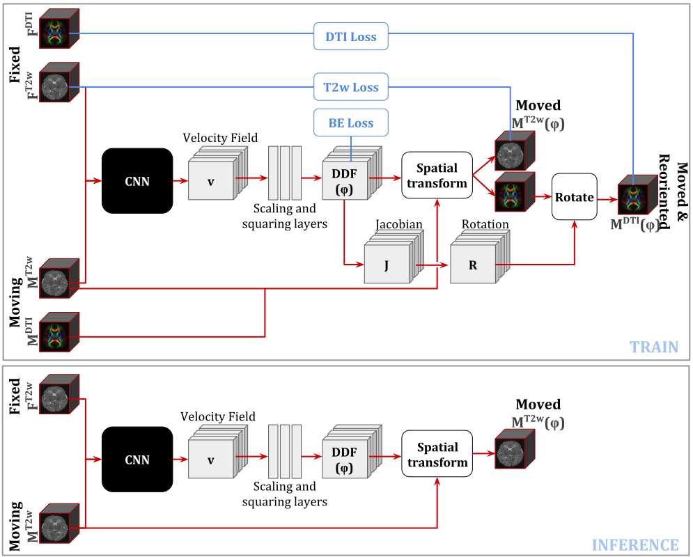
Figure 1: The proposed network architecture at both training and inference time.

The model is trained using stochastic gradient descent to find the optimal parameters $\hat{\theta}$ that minimize a sum of three loss functions, representing the tensor similarity measure, the scalar-data similarity measure and a regulariser applied on the predicted deformation field. The dti data is not used as input to our cnn, but only used to drive the learning process through calculating the similarity measure. During inference, our model uses only t2w images to predict the deformation field, without the need for a second modality. In the following subsections, we describe our model in further detail.

Network architecture

The baseline architecture of our network is a 3-D UNet [12] based on VoxelMorph [2]. The encoding branch is made up of four 3D convolutions of $16,32,32$, and $32$ filters, respectively, with a kernel size of $3\times 3\times 3$, followed by Leaky ReLU ($\alpha=0.2$) activations [18]. The decoding branch contains four transverse 3D convolutions of 32 filters each, with the same kernel size and activation function. Skip connections are used to concatenate the encoding branch’s information to the decoder branch. Two more convolutional layers, one with $16$ filters and a second one with $3$ filters, are added at the end, both with the same kernel size and activation function as before.

A pair of t2w images are concatenated on the channel axis and become a $96\times 96\times 64\times 2$ input for the cnn network. The output is a three channel velocity field of the same size as the input images. The velocity field is smoothed with a $3\times 3\times 3$ Gaussian kernel (with $\sigma=1.2$ mm), and passed onto seven squaring and scaling layers [2], which transform it into a topology-preserving deformation field. The SpatialTransform layer [5] receives as input the predicted field $\phi$ and the moving scalar-valued t2w image, and outputs the warped and resampled image. A similar process is necessary to warp the moving dt image, with a few extra steps which are explained in the next subsection.

Tensor reorientation

Registration of dt images is not as straightforward to perform as scalar-valued data. When transforming the latter, the intensities in the moving image are interpolated at the new locations determined by the deformation field $\phi$ and copied to the corresponding location in the target image space. However, after interpolating dt images, the diffusion tensors need to be reoriented to remain anatomically correct [1]. In this work we use the finite strain (FS) strategy [1].

When the transformation is non-linear, such as in our case, the reorientation matrix can be computed at each point in the deformation field $\phi$ through a polar decomposition of the local Jacobian matrix. This factorisation transforms the non-singular matrix $J$ into a unitary matrix $R$ (the pure rotation) and a positive-semidefinite Hermitian matrix $P$, such that $J=RP$ [15]. The rotation matrices $R$ are then used to reorient the tensors without changing the local microstructure.

Loss function

We train our model using a loss function composed of three parts. First, the structural loss $\mathcal{L}_{struct}$ (applied on the t2w data only) is a popular similarity measure used in medical image registration, called ncc. We define it as:

$$NCC(F,M(\phi))=-\frac{\sum_{\mathbf{x}\in\Omega}(F(\mathbf{x})-\overline{F})\cdot(M(\phi(\mathbf{x}))-\overline{M})}{\sqrt{\sum_{\mathbf{x}\in\Omega}(F(\mathbf{x})-\overline{F})^{2}\cdot\sum_{\mathbf{x}\in\Omega}(M(\phi(\mathbf{x}))-\overline{M})^{2}}}$$

where $\overline{F}$ is the mean voxel value in the fixed image $F$ and $\overline{M}$ is the mean voxel value in the transformed moving image $M(\phi)$.

Second, to encourage a good alignment between the dt images, we set $\mathcal{L}_{tensor}$ to be one of the most commonly used diffusion tensor similarity measures, known as the Euclidean distance squared. We define it as:

$$EDS(F,M(\phi))=\sum_{\mathbf{x}\in\Omega}\lvert\lvert F(\mathbf{x})-M(\phi(\mathbf{x}))\rvert\rvert_{C}^{2}$$

where the euclidean distance between two pairs of tensors $\mathbf{D_{1}}$ and $\mathbf{D_{2}}$ is defined as $\lvert\lvert\mathbf{D_{1}}-\mathbf{D_{2}}\rvert\rvert_{C}=\sqrt{Tr((\mathbf{D_{1}}-\mathbf{D_{2}})^{2})}$ [19].

Finally, to ensure a smooth deformation field $\phi$ we use a regularisation penalty $\mathcal{L}_{reg}$ in the form of bending energy [13]:

$$BE(\phi)=\sum_{\mathbf{x}\in\Omega} \Big{[}\Big{(}\frac{\partial^{2}\phi(\mathbf{x})}{\partial x^{2}}\Big{)}^{2}+\Big{(}\frac{\partial^{2}\phi(\mathbf{x})}{\partial y^{2}}\Big{)}^{2}+\Big{(}\frac{\partial^{2}\phi(\mathbf{x})}{\partial z^{2}}\Big{)}^{2}+$$

$$2\Big{(}\frac{\partial^{2}\phi(\mathbf{x})}{\partial xy}\Big{)}^{2}+2\Big{(}\frac{\partial^{2}\phi(\mathbf{x})}{\partial xz}\Big{)}^{2}+2\Big{(}\frac{\partial^{2}\phi(\mathbf{x})}{\partial yz}\Big{)}^{2}\Big{]}$$

Thus, the final loss function is:

$$\mathcal{L}(F,M(\phi))=\alpha\,EDS(F^{DTI},M^{DTI}(\phi))+\beta\,NCC(F^{T2w},M^{T2w}(\phi))+\lambda\,BE(\phi)$$

We compare our network with a baseline trained on t2w data only. For the latter case the loss function becomes: $\mathcal{L}(F,M(\phi))=\beta\,NCC(F^{T2w},M^{T2w}(\phi))+\lambda\,BE(\phi)$. In all of our experiments we set the weights to $\alpha=1.0$, $\beta=1.0$ and $\lambda=0.001$ when using both dti and t2w images, and to $\beta=1.0$ and $\lambda=0.001$ when using t2w data only. These hyper-parameters were found to be optimal on our validation set.

3 Experiments

Dataset

The image dataset used in this work is part of the developing Human Connectome Project. Both the t2w images and the dw images were acquired using a 3T Philips Achieva scanner and a 32-channels neonatal head coil [6]. The structural data was acquired using a turbo spin echo (TSE) sequence in two stacks of 2D slices (sagittal and axial planes), with parameters: $T_{R}=12$ s, $T_{E}=156$ ms, and SENSE factors of 2.11 for the axial plane and 2.58 for the sagittal plane. The data was subsequently corrected for motion [4, 8] and resampled to an isotropic voxel size of $0.5$ mm.

The dw images were acquired using a monopolar spin echo echo-planar imaging (SE-EPI) Stejksal-Tanner sequence [7]. A multiband factor of 4 and a total of 64 interleaved overlapping slices ($1.5$ mm in-plane resolution, $3$ mm thickness, $1.5$ mm overlap) were used to acquire a single volume, with parameters $T_{R}=3800$ ms, $T_{E}=90$ ms. This data underwent outlier removal, motion correction and it was subsequently super-resolved to a $1.5$ mm isotropic voxel resolution [3]. All resulting images were checked for abnormalities by a paediatric neuroradiologist.

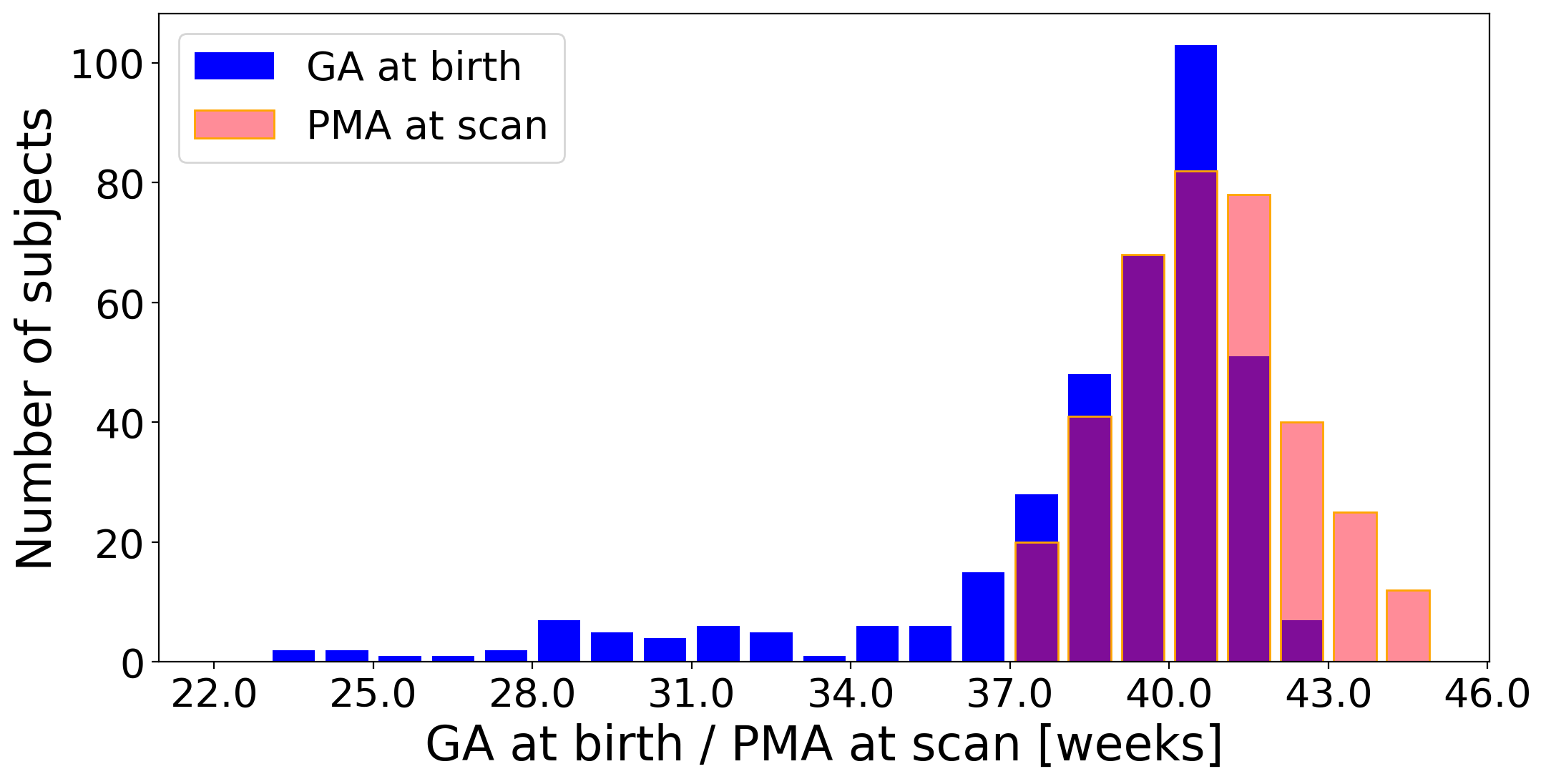
Figure 2: Distribution of gestational ages at birth (GA) and post-menstrual ages at scan (PMA) in our dataset.

For this study, we use a total of 368 t2w and dt volumes of neonates born between $23-42$ weeks ga and scanned at term-equivalent age ($37-45$ weeks ga). The age distribution in our dataset is found in Figure 2, where ga at birth is shown in blue, and pma at scan is shown in orange. In order to use both the t2w and dt volumes in our registration network, we first resampled the t2w data into the dw space of $1.5$ mm voxel resolution. Then, we affinely registered all of our data to a common 40 weeks gestational age atlas space [14] available in the MIRTK software toolbox [13] and obtained the dt images using the dwi2tensor [17] command available in the MRTRIX toolbox. Finally, we performed skull-stripping using the available dHCP brain masks [3] and we cropped the resulting images to a $96\times 96\times 64$ volume size.

Training

We trained our models using the rectified Adam (RAdam) optimiser [9] with a cyclical learning rate [16] varying from $10^{-9}$ to $10^{-4}$, for $90,000$ iterations. Out of the 368 subjects in our entire dataset, 318 were used for training, 25 for validation and 25 for test. The subjects in each category were chosen such that their ga at birth and pma at scan were distributed across the entire range. The validation set was used to help us choose the best hyperparameters for our network and the best performing models. The results reported in the next section are on the test set.

Final model results

In both our t2w-only and t2w+dti cases we performed a leave-one-out cross-validation, where we aligned 24 of the test subjects to a single subject, and repeated until all the subjects were used as target. Each of the 25 subjects had tissue label segmentations (obtained using the Draw-EM pipeline for automatic brain MRI segmentation of the developing neonatal brain [10]) which were propagated using NiftyReg [11] and the predicted deformation fields. The average resulting Dice scores are summarised in Figure 3, where the initial pre-alignment is shown in pink, the t2w-only results are shown in light blue and the t2w+dti are shown in purple. Our proposed model performs better than the baseline model for all subcortical structures (cerebellum, deep gray matter, brainstem and hippocampi and amygdala), while performing similarly well in white matter structures. In contrast, cortical gray matter regions were better aligned when using the t2w-only model, as structural data has higher contrast than DTI in these areas.

We also computed the FA maps for all the initial affinely aligned and all the warped subjects in the cross-validation study and calculated the sum-of-squared differences (SSD) between the moved FA maps and the fixed FA maps. The resulting average values are summarised in Table 1, which shows that our proposed model achieved better alignment in terms of FA maps.

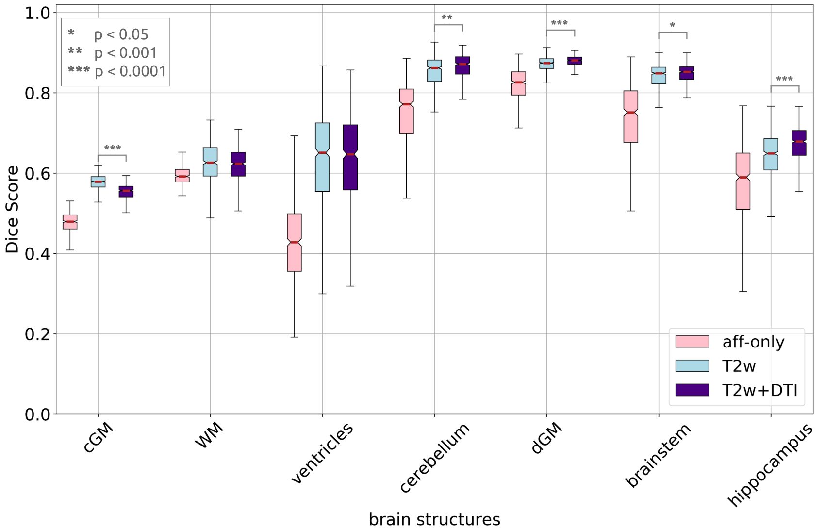
Figure 3: Average Dice scores for our cross-validation study for 7 tissue types: cortical gray matter (cGM), white matter (WM), ventricles, cerebellum, deep gray matter (dGM), brainstem and the hippocampus. For both of our trained models the input images, $F^{T2w\lvert DTI}$ and $M^{T2w\lvert DTI}$, have been affinely aligned to a template, prior to being used by the models. Our proposed model outperforms the t2w-only training in terms of obtaining higher Dice scores for the cerebellum, dGM, brainstem and hippocampus.

Method	Mean(SSD)	Std.Dev.(SSD)	p-value
Affine	1087	174	Affine	vs	T2w	$p<1e^{-5}$
T2w	1044	168	Affine	vs	T2w+DTI	$p<1e^{-5}$
T2w+DTI	981	181	T2w	vs	T2w+DTI	$p<1e^{-5}$

Table 1: Average sum-of-squared differences between warped and fixed FA maps in our leave-one-out cross-validation study. The first line shows mean and standard deviation SSD values for the initial affine alignment.

Finally, Figure 4 shows two example registrations. The target images are from two term-born infants with GA = 40.86 weeks and PMA = 41.43 weeks, and GA = 40.57w and PMA = 41w, respectively, while the moving images are from infants with GA = 40.57 weeks and PMA = 41 weeks, and GA = 37.14w and PMA = 37.28w, respectively. The figure shows both t2w and FA maps of axial slices of the fixed (first column), the moving (second column) and the warped images by our proposed method (third column) and the baseline method (fourth column), respectively. The moved FA maps show that by using dti data to drive the learning process of a deep learning registration framework, we were able to achieve good alignment not only on the structural data, but also on the diffusion data as well.

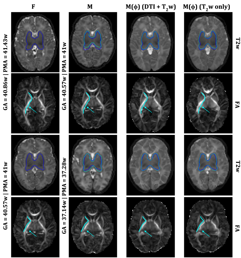
Figure 4: First two rows show an example registration between a neonate with GA = 40.57w and PMA = 41w as moving, and one with GA = 40.86w and PMA = 41.43w as fixed, last two rows show an example where the moving image is from a neonate with GA = 37.14w and PMA = 37.28w, and fixed is a neonate with GA = 40.57w and PMA = 41w. First column shows axial slices of the fixed t2w images and FA maps, the second column shows axial slices of the moving t2w images and FA maps, and the third and fourth columns show the moved images using our proposed network and the baseline network, respectively. In the t2w maps the deep gray matter (dGM) labels are shown for the fixed images in dark blue and for the moving and moved in cyan. In both cases a higher dGM Dice score was obtained for the t2w+dti model (0.88 and 0.88, respectively), than when using t2w-only (0.84 and 0.87, respectively). The arrows point at areas where the underlying anatomy was better preserved when using t2w+dti, than when using t2w-only.

4 Discussion and future work

In this work we showed for the first time a deep learning registration framework capable of aligning both structural (T2w) and microstructural (DTI) data, while using only t2w data at inference time. A key result from our study is that our proposed t2w+dti model performed better in terms of aligning subcortical structures, even though the labels for these regions were obtained from structural data only. For future work we plan to focus on improving the registration in the cortical regions, and to compare our deep learning model with classic registration algorithms.

References

- [1] Alexander, D.C., Pierpaoli, C., Basser, P.J., Gee, J.C.: Spatial transformations of diffusion tensor magnetic resonance images. IEEE transactions on medical imaging 20(11), 1131–1139 (2001)
- [2] Balakrishnan, G., Zhao, A., Sabuncu, M.R., Guttag, J., Dalca, A.V.: Voxelmorph: A learning framework for deformable medical image registration. IEEE Transactions on Medical Imaging 38(8), 1788–1800 (Aug 2019)
- [3] Christiaens, D., Cordero-Grande, L., Pietsch, M., Hutter, J., Price, A.N., Hughes, E.J., Vecchiato, K., Deprez, M., Edwards, A.D., Hajnal, J.V., et al.: Scattered slice shard reconstruction for motion correction in multi-shell diffusion MRI of the neonatal brain. arXiv preprint arXiv:1905.02996 (2019)
- [4] Cordero-Grande, L., Hughes, E.J., Hutter, J., Price, A.N., Hajnal, J.V.: Three-dimensional motion corrected sensitivity encoding reconstruction for multi-shot multi-slice MRI: Application to neonatal brain imaging. Magnetic Resonance in Medicine 79(3), 1365–1376 (2018)
- [5] Dalca, A.V., Balakrishnan, G., Guttag, J., Sabuncu, M.R.: Unsupervised learning for fast probabilistic diffeomorphic registration. Lecture Notes in Computer Science p. 729–738 (2018)
- [6] Hughes, E.J., Winchman, T., Padormo, F., Teixeira, R., Wurie, J., Sharma, M., Fox, M., Hutter, J., Cordero-Grande, L., Price, A.N., Allsop, J., Bueno-Conde, J., Tusor, N., Arichi, T., Edwards, A.D., Rutherford, M.A., Counsell, S.J., Hajnal, J.V.: A dedicated neonatal brain imaging system. Magnetic Resonance in Medicine 78(2), 794–804 (2017)
- [7] Hutter, J., Tournier, J.D., Price, A.N., Cordero-Grande, L., Hughes, E.J., Malik, S., Steinweg, J., Bastiani, M., Sotiropoulos, S.N., Jbabdi, S., et al.: Time-efficient and flexible design of optimized multishell hardi diffusion. Magnetic resonance in medicine 79(3), 1276–1292 (2018)
- [8] Kuklisova-Murgasova, M., Quaghebeur, G., Rutherford, M.A., Hajnal, J.V., Schnabel, J.A.: Reconstruction of fetal brain MRI with intensity matching and complete outlier removal. Medical image analysis 16(8), 1550–1564 (2012)
- [9] Liu, L., Jiang, H., He, P., Chen, W., Liu, X., Gao, J., Han, J.: On the variance of the adaptive learning rate and beyond (2019)
- [10] Makropoulos, A., Gousias, I.S., Ledig, C., Aljabar, P., Serag, A., Hajnal, J.V., Edwards, A.D., Counsell, S.J., Rueckert, D.: Automatic whole brain MRI segmentation of the developing neonatal brain. IEEE transactions on medical imaging 33(9), 1818–1831 (2014)
- [11] Modat, M., Ridgway, G.R., Taylor, Z.A., Lehmann, M., Barnes, J., Hawkes, D.J., Fox, N.C., Ourselin, S.: Fast free-form deformation using graphics processing units. Computer methods and programs in biomedicine 98(3), 278–284 (2010)
- [12] Ronneberger, O., Fischer, P., Brox, T.: U-net: Convolutional networks for biomedical image segmentation. Medical Image Computing and Computer-Assisted Intervention – MICCAI 2015 p. 234–241 (2015)
- [13] Rueckert, D., Sonoda, L.I., Hayes, C., Hill, D.L.G., Leach, M.O., Hawkes, D.J.: Nonrigid registration using free-form deformations: application to breast MR images. IEEE Transactions on Medical Imaging 18(8), 712–721 (1999)
- [14] Schuh, A., Makropoulos, A., Robinson, E.C., Cordero-Grande, L., Hughes, E., Hutter, J., Price, A.N., Murgasova, M., Teixeira, R.P.A.G., Tusor, N., Steinweg, J.K., Victor, S., Rutherford, M.A., Hajnal, J.V., Edwards, A.D., Rueckert, D.: Unbiased construction of a temporally consistent morphological atlas of neonatal brain development. bioRxiv (2018)
- [15] Shoemake, K., Duff, T.: Matrix animation and polar decomposition. In: Proceedings of the conference on Graphics interface. vol. 92, pp. 258–264. Citeseer (1992)
- [16] Smith, L.N.: Cyclical learning rates for training neural networks (2015)
- [17] Veraart, J., Sijbers, J., Sunaert, S., Leemans, A., Jeurissen, B.: Weighted linear least squares estimation of diffusion MRI parameters: strengths, limitations, and pitfalls. NeuroImage 81, 335–346 (2013)
- [18] Xu, B., Wang, N., Chen, T., Li, M.: Empirical evaluation of rectified activations in convolutional network (2015)
- [19] Zhang, H., Yushkevich, P.A., Alexander, D.C., Gee, J.C.: Deformable registration of diffusion tensor mr images with explicit orientation optimization. Medical image analysis 10(5), 764–785 (2006)