Two-pole structures in QCD: Facts, not fantasy!

Abstract

The two-pole structure refers to the fact that particular single states in the spectrum as listed in the PDG tables are often two states. The story began with the $\Lambda(1405)$, when in 2001, using unitarized chiral perturbation theory, it was observed that there are two poles in the complex plane, one close to the $\bar{K}p$ and the other close to the $\pi\Sigma$ threshold. This was later understood combining the SU(3) limit and group-theoretical arguments. Different unitarization approaches that all lead to the two-pole structure have been considered in the mean time, showing some spread in the pole positions. This fact is now part of the PDG book, though it is not yet listed in the summary tables. Here, I will discuss the open ends and critically review approaches that can not deal with this issue. In the meson sector some excited charm mesons are good candidates for such a two-pole structure. Next, I consider in detail the $D_{0}^{*}(2300)$, that is another candidate for this scenario. Combining lattice QCD with chiral unitary approaches in the finite volume, the precise data of the Hadron Spectrum Collaboration for coupled-channel $D\pi$, $D\eta$, $D_{s}\bar{K}$ scattering in the isospin $I=1/2$ channel indeed reveal its two-pole structure. Further states in the heavy meson sector with $I=1/2$ exhibiting this phenomenon are predicted, especially in the beauty meson sector. I also discuss the relation of these two-pole structures and the possible molecular nature of the states under consideration.

1 Introduction

The hadron spectrum is arguably the least understood part of Quantum Chromodynamics (QCD), the theory of the strong interactions. It is part of the successful Standard Model (SM) and thus, we can say that structure formation, that is the emergence of hadrons and nuclei from the underlying quark and gluon degrees of freedom, is indeed the last corner of the SM that is not yet understood. For a long time, the quark model of Gell-Mann [1] and Zweig [2] (and many sophisticated extensions thereof, such as [3]) have been used to bring order into the particle zoo. However, already before QCD it was a puzzling fact that all observed hadrons could be described by the simplest combinations of quarks/antiquarks, namely mesons as quark-antiquark states and baryons as three quark states, while symmetries and quantum numbers would also allow for tetraquarks, pentaquarks and so on. The situation got even worse when QCD finally appeared on the scene, as it allows for the following structures (bound systems of quarks and/or gluons):

• Conventional hadrons, that is mesons and baryons as described before;

• Multiquark hadrons, like tetraquark states (mesons from two quarks and two antiquarks), pentaquark states (baryons made from four quarks and one antiquark), and so on;

• Hadronic molecules and atomic nuclei, that is multiquark states composed of a certain number of conventional hadrons (as discussed in more detail below);

• Hybrid states, which are composed of quarks and (valence) gluons;

• Glueballs, bound states solely made of gluons, arguably the most exotic form of matter, which has so far been elusive in all searches.

The observed hadrons are listed with their properties in the tables of the Particle Data Group (PDG) (also called “Review of Particle Physics” (RPP)) [4] within a certain rating scheme, just telling us that some states are better understood as others. What complicates matters a lot is the fact that almost all hadrons are resonances, that is unstable states. These decay into other hadrons and leptons, like e.g. the $\rho$ meson decays into two pions or into a pion and a photon (and other final states). Such a resonance is thus described by a complex energy, more precisely, the real part is called the mass, $m_{R}$, and the imaginary part the half-width, $\Gamma_{R}/2$. Consequently, all other properties are also given by complex numbers. The only model-independent way to pin down these basic resonance properties is to look for poles in the complex plane, where resonances are usually located on the second Riemann sheet at

$$z_{R}=(\Re z_{R},\textrm{Im}\,z_{R})=(m_{R},\Gamma_{R}/2)~{}.$$ (1)

The residues at these poles contain information about the possible decays of such a resonance, as will be discussed in more detail below.

As I will discuss in what follows, the hunt for such poles in the complex plane has revealed the astonishing feature of the two-pole structure, namely that certain states that are listed in the RPP are indeed superpositions of two states. The most prominent example is the $\Lambda(1405)$, which is discussed in detail in Sect. 3. More recently, the $D_{0}^{*}(2300)$, an excited charm meson, has become another prime candidate for the two-pole scenario, paving the way for a whole set of such states in the heavy-light sector (mesons made of one light $(u,d,s)$ and one heavy $(c,b)$ quark), see Sect. 4. Before discussing these intricate states, it is, however, necessary to review the pertinent methods underlying the theoretical analyses, see Sect. 2. The conclusions and outlook are given in Sect. 5.

2 Methods

We start with the Lagrangian of QCD for up, down and strange quarks ($N_{f}=3$), which can be written as:

$${\cal L}_{\rm QCD} = {\cal L}^{0}_{\rm QCD}-\bar{q}{\cal M}q~{},$$

$${\cal L}^{0}_{\rm QCD} = -\frac{1}{2g^{2}}{\rm Tr}\left[G_{\mu\nu}G^{\mu\nu}\right]+\bar{q}i\gamma^{\mu}(\underbrace{\partial_{\mu}-iA_{\mu}}_{=D_{\mu}})q~{}.$$ (2)

Here, $q=(u,d,s)^{T}$ is the quark triplet, $A_{\mu}$ is the gluon field, $G_{\mu\nu}$ the gluon field strength tensor, $g$ is the strong coupling constant and the color indices related to the underlying SU(3)_c local gauge symmetry have not been displayed. Further, ${\cal M}={\rm diag}(m_{u},m_{d},m_{s})$ is the quark matrix and the heavy flavors charm and bottom can be added analogously. Also, gauge fixing and the CP-violating $\theta$-term are not displayed. Remarkably, ${\cal L}^{0}_{\rm QCD}$ displays a SU(3)$\times$SU(3) flavor symmetry (I do not discuss the additional U(1) symmetries/non-symmetries here),

$${\cal L}^{0}_{\rm QCD}(G_{\mu\nu},q^{\prime},D_{\mu}q^{\prime})={\cal L}^{0}_{\rm QCD}(G_{\mu\nu},q,D_{\mu}q)~{},$$ (3)

in terms of left- and right-handed quark fields,

$$q^{\prime}=g_{R}P_{R}q+g_{L}P_{L}q~{},~{}~{}P_{R,L}=\frac{1}{2}(1\pm\gamma_{5})~{},~{}~{}g_{I}g^{\dagger}_{I}=\mathds{1}~{},~{}~{}{\rm det}g_{I}=1~{},~{}~{}I=L,R~{}.$$ (4)

This is the chiral symmetry of QCD. It leads to $16=2\cdot(N_{f}^{2}-1)$ conserved Noether currents, that can be rearranged as 8 conserved vector and 8 conserved axial-vector currents. However, we know that the symmetry of the groundstate is not the symmetry of the QCD Hamiltonian, as e.g. there is no parity-doubling in the spectrum. The symmetry is spontaneously broken (or hidden, as Nambu preferred to say) to its vectorial subgroup:

$${\rm SU(3)}_{L}\times{\rm SU(3)}_{R}\to{\rm SU(3)}_{V}~{}.$$ (5)

The Goldstone theorem then tells us that for each broken generator there should be a massless boson (the famous Goldstone bosons). Therefore, in the absence of quark masses, we are dealing with a theory without a mass gap, which implies that Taylor expansions are not analytic. When the quark masses are included, the pseudoscalar Goldstone bosons acquire a small mass. In fact, the lightest hadrons are the eight pseudoscalar mesons ($\pi,K,\eta$). All this is the basis for the formulation of an effective field theory (EFT), that allows for perturbative calculations at low energy. Similarly, for the heavy quarks $c$ and $b$ one can formulate a different EFT, based on the fact that the $c$ ad $b$ masses are large, $m_{c,b}\gg\Lambda_{\rm QCD}$, as discussed next.

2.1 Limits of QCD

We have just discussed one particular limit of QCD, namely the chiral limit of the three light flavor theory. Such a special formulation can be extended also to the heavy quark sector and to so-called heavy-light systems. The various limits of QCD are:

• Light quarks:

  $${\cal L}_{\rm QCD}=\bar{q}_{L}\,iD\!\!\!\!/\,q_{L}+\bar{q}_{R}\,iD\!\!\!\!/\,q_{R}+{\cal O}(m_{f}/\Lambda_{\rm QCD})~{}~{}~{}[f=u,d,s]~{}.$$ (6)

  In this limit, left- and right-handed quarks decouple which is the chiral symmetry. As stated, it is spontaneously broken leading to the appearance of 8 pseudo-Goldstone bosons. The pertinent EFT is chiral perturbation theory (CHPT), see Sect. 2.2. Note that the corrections due to the quark masses are powers in $m_{f}$.

• Heavy quarks:

  $${\cal L}_{\rm QCD}=\bar{Q}_{f}\,iv\cdot D\,Q_{f}+{\cal O}(\Lambda_{\rm QCD}/m_{f})~{}~{}~{}[f=c,b]~{},$$ (7)

  where $Q$ denotes the field of a heavy quark. In this limit, the Lagrangian is independent of quark spin and flavor, which leads to SU(2) spin and SU(2) flavor symmetries, called HQSS and HQFS, respectively. The pertinent EFT is heavy quark effective field theory (HQEFT), see e.g. [5, 6]. Here, the corrections due to the quark masses are powers in $1/m_{Q}$.

• Heavy-light systems: Here, heavy quarks act as matter fields coupled to light pions and one thus can combine CHPT and HQEFT as pioneered in [7, 8, 9], see also Sect. 2.3.

2.2 A factsheet on chiral perturbation theory

Chiral perturbation theory is the EFT of QCD at low energies [11, 10]. For introduction and reviews, see e.g. [12, 13, 14]. Its basic properties are:

• ${\cal L}$ is symmetric under some Lie group ${\cal G}$, here ${\cal G}$ = SU(3)${}_{L}\times$ SU(3)_R.

• The ground state $|0\rangle$ is asymmetric and ${\cal G}$ is spontaneously broken to ${\cal H}\subset{\cal G}$, leading to the the appearance of Goldstone bosons (GBs) $|\phi^{i}(p)\rangle$. In QCD, ${\cal H}$ = SU(3)_V and the Goldstone bosons are the aforementioned eight pseudoscalar mesons.

• In QCD, the matrix element of the axial-vector current ${\cal A}_{\mu}^{i}$, $\langle 0|{\cal A}_{\mu}^{i}|\phi^{k}(p)\rangle=i\delta^{ik}p_{\mu}F\neq 0$ $(i=1,\ldots,8)$, where $F$ is related to the pseudoscalar decay constant in the chiral limit. $F\neq 0$ is a sufficient and necessary condition for spontaneous chiral symmetry breaking.

• There are no other massless strongly interacting particles.

Universality tells us that at low energies, any theory with these properties looks the same as long as the number of space-time dimensions is larger than two. One can readily deduce that the interactions of the GBs are weak in the low-energy regime and indeed vanish at zero energy. This allows for a systematic expansion in small momenta and energies, and the quark masses lead to finite but small GB masses, which defines a second expansion parameter. In fact, these two parameters can be merged in one. The corresponding effective Lagrangian is readily constructed, it takes the form

$${\cal L}_{\rm eff}={\cal L}^{(2)}+{\cal L}^{(4)}+{\cal L}^{(6)}+\ldots\,,$$ (8)

where the superscript denotes the power of the small expansion parameter $p$ (derivatives and/or GB mass insertions). This expansion is systematic, as an underlying power counting [11] can be derived. This shows that graphs with $n$ loops are suppressed by powers of $p^{2n}$ and that at each order, we have local operators accompanied by unknown coupling constants, also called low-energy constants (LECs). These LECs must be determined from fits to experimental data or can be calculated using lattice QCD. Their specific values single out QCD from the whole universality class of theories discussed above. One important issue concerns unitarity. Leading order calculations are based on tree diagrams with insertions from ${\cal L}^{(2)}$, which means that such amplitudes are real. Imaginary parts are only generated at one-loop order through the loop diagrams, which means that unitarity is fulfilled perturbatively but not exactly in CHPT, for a general discussion, see [15]. We will come to this issue in Sect. 2.4.

Matter fields like baryons can also be included in a systematic fashion. There is one major complication, namely the matter field mass that is of the same size as the breakdown scale of the EFT, here $\Lambda_{\chi}\sim 1\,$GeV. Therefore, only three-momenta of the matter fields can be small and the mass must be dealt with in some manner. Various schemes like the heavy baryon approach [16, 17], infrared regularization [18] and the extended on-mass-shell scheme [19] exist to restore the power counting. For details, I refer to the reviews [20, 21, 22].

2.3 Chiral perturbation theory for heavy-light systems

In this section, we display the effective Lagrangians that we need for the discussion of charm mesons and their interactions. Consider first Goldstone boson scattering off $D$-mesons. The effective Lagrangian takes the form [23, 24, 25]:

$${\cal L}_{\rm eff} = {\cal L}^{(1)}+{\cal L}^{(2)}~{},$$

$${\cal L}^{(1)} = {\cal D}_{\mu}D{\cal D}^{\mu}D^{\dagger}-M_{D}^{2}DD^{\dagger}~{},$$

$${\cal L}^{(2)} = D\left[-h_{0}\langle\chi_{+}\rangle-h_{1}\chi_{+}+h_{2}\langle u_{\mu}u^{\mu}\rangle-h_{3}u_{\mu}u^{\mu}\right]\bar{D}+{\cal D}_{\mu}D\left[h_{4}\langle u^{\mu}u^{\nu}\rangle-h_{5}\{u^{\mu},u^{\nu}\}\right]{\cal D}_{\nu}\bar{D}~{}.$$ (9)

Here, $D=(D^{0},D^{+},D_{s}^{+})$ is the $D$-meson triplet, $M_{D}$ the average mass of the $D$-mesons, and we utilize the standard chiral building blocks $u_{\mu}\sim\partial_{\mu}\phi$, with $\phi$ a member of the GB octet, and $\chi_{+}\sim{\rm diag}(m_{u},m_{d},m_{s})$. The pertinent LECs can all be determined: $h_{1}=0.42$ from the $D_{s}$-$D$ splitting, while $h_{2,3,4,5}$ are fixed from a fit to lattice data [26]. Further, $h_{0}$ can be fixed from the pion mass dependence of the $D$ meson masses.

In what follows, we will also consider $\bar{B}\to D$ transitions with the emission of two light pseudoscalars (pions). Here, chiral symmetry puts constraints on one of the two pions while the other one moves fast and does not participate in the final-state interactions. The corresponding chiral effective Lagrangian has been developed in Ref. [27]:

$${\cal L}_{\rm eff} = \bar{B}\big{[}c_{1}\left(u_{\mu}tM+Mtu_{\mu}\right)+c_{2}\left(u_{\mu}M+Mu_{\mu}\right)t+c_{3}\,t\left(u_{\mu}M+Mu_{\mu}\right)$$ (10)

$$+ c_{4}\left(u_{\mu}\langle Mt\rangle+M\langle u_{\mu}t\rangle\right)+c_{5}\,t\langle Mu_{\mu}\rangle+c_{6}\langle\left(Mu_{\mu}+u_{\mu}M\right)t\rangle\big{]}\partial^{\mu}D^{\dagger}~{},$$

in terms of the $B$-meson triplet $\bar{B}=(B^{-},\bar{B}^{0},\bar{B}_{s}^{0})$, $M$ is the matter field for the fast-moving pion and $t=uHu$ is a spurion field for Cabbibo-allowed decays,

$$H=\begin{pmatrix}0&0&0\\ 1&0&0\\ 0&0&0\end{pmatrix}~{}.$$ (11)

In the $B\to D\pi\pi$ decays that we will discuss later, only some combinations of the LECs $c_{i}$ ($i=1,\ldots,6$) appear, see Sect. 4.3.

2.4 Unitarization schemes

As stated before, unitarity is only fulfilled perturbatively in CHPT. The hard scale in this EFT is set by the appearance of resonances, like the $f_{0}(500)$ or the $\rho(770)$ in various partial waves of pion-pion scattering. CHPT is thus not the proper framework to describe resonances. One possible way to extend the energy region where this can be applied is unitarization, originally proposed in Ref. [28]. However, this comes at a price, usually crossing symmetry is violated in such type of approach and the coefficient of subleading chiral logarithms are often incorrectly given, see [15]. Here, let us just discuss a familiar approach on solving the Bethe-Salpeter equation in the on-shell approximation, see e.g [39, 40]. To be specific, let us consider the coupled-channel process $\phi+D\to\phi+D$ (suppressing all indices). The basic unitarization method is depicted in Fig. 1. It amounts to a resummation of the so-called “fundamental bubble” (the 2-point loop function). To describe resonances like e.g. the $D_{s0}^{*}(2317)$, one has to search for poles of the $T$-matrix, which is generated from the CHPT potential by unitarization.

Figure 1: The $T$-matrix for GB (dashed lines) scattering off $D$-mesons (solid lines) as a bubble sum based on the effective potential $V$, that is obtained from the underlying chiral effective Lagrangian.

This version of unitarized CHPT is based on the fundamental equation

$$T^{-1}(s)=V^{-1}(s)-G(s)~{},$$ (12)

where $V(s)$ is derived from the effective Lagrangian Eq. (2.3) and $G(s)$ is the 2-point scalar loop function regularized by a subtraction constant ${a}(\mu)$,

$$G(s) \!= \!\frac{1}{16\pi^{2}}\bigg{\{}{a}(\mu)+\ln{\frac{m_{2}^{2}}{\lambda^{2}}}+\frac{m_{1}^{2}-m_{2}^{2}+s}{2s}\ln{\frac{m_{1}^{2}}{m_{2}^{2}}}+\frac{\sigma}{2s}\left[\ln({s-m_{1}^{2}+m_{2}^{2}+\sigma})\right.$$ (13)

$$\left.-\ln({-s+m_{1}^{2}-m_{2}^{2}+\sigma})+\ln({s+m_{1}^{2}-m_{2}^{2}+\sigma})-\ln({-s-m_{1}^{2}+m_{2}^{2}+\sigma})\right]\bigg{\}},$$

with $\sigma=\left\{[s-(m_{1}+m_{2})^{2}][s-(m_{1}-m_{2})^{2}]\right\}^{1/2}$ and $m_{1}$ and $m_{2}$ are the masses of the two mesons in the loop, here one $D$-meson and one GB. $\mu$ is the scale of dimensional regularization, and a change of $\mu$ can be absorbed by a corresponding change of ${a}(\mu)$. Promoting $T(s)$, $V(s)$ and $G(s)$ to be matrix-valued quantities, it is easy to generalize Eq. (12) to coupled channels. More details on the unitarization schemes will be given in the subsequent sections.

2.5 Unitarized chiral perturbation theory in a finite volume

To compare with lattice data, we need to formulate the unitarization scheme in a finite volume (FV). Obviously, in any FV scheme, momenta are no longer continuous but quantized,

$$\vec{q}=\displaystyle\frac{2\pi}{L}\vec{n}~{},~{}~{}\vec{n}\in\mathbb{Z}^{3}~{},$$ (14)

in a cubic volume of length $L$, i.e. $V=L^{3}$. An appropriate FV representation of the scalar 2-point function is (see Ref. [29] for details)

$$\tilde{G}(s,L)=\displaystyle\lim_{\Lambda\to\infty}\left[\frac{1}{L^{3}}\sum_{\vec{n}}^{|\vec{q}|<\Lambda}I(\vec{q}\,)-\int_{0}^{\Lambda}\frac{q^{2}dq}{2\pi^{2}}I(\vec{q}\,)\right]~{},$$ (15)

with $I(\vec{q}\,)$ the corresponding integrand. The FV energy levels of the process under consideration are then obtained from the poles of $\tilde{T}(s,L)$:

$$\tilde{T}^{-1}(s,L)=V^{-1}(s)-\tilde{G}(s,L)~{}.$$ (16)

Note that all volume dependence resides in $\tilde{G}(s,L)$, the effective Lagrangian and thus the effective potential are the same as in the continuum [30]. Again, in case of coupled channels, Eq. (16) is promoted to a matrix equation.

3 The story of the $\Lambda(1405)$

3.1 Basic facts

In the quark model, the $\Lambda(1405)$ is a $uds$ excitation with $J^{P}=1/2^{-}$ a few hundred MeV above the ground-state $\Lambda(1116)$. The RPP gives one corresponding state with

$$m=1405.1^{+1.3}_{-1.0}~{}{\rm MeV}\,,~{}\Gamma=50.5\pm 2.0\,{\rm MeV}~{}.$$ (17)

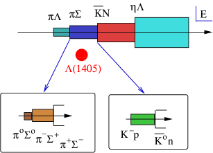
Figure 2: Complex energy plane in the vicinity of the $\Lambda(1405)$.

In fact, the $\Lambda(1405)$ was predicted long before the quark model as a resonance in the coupled $\pi\Sigma$ and $\bar{K}N$ channels, see [31] and also [32], and considered as a $\bar{K}N$ bound state, arguably the first “exotic” hadron ever. The analytical structure in the complex energy plane between the $\pi\Lambda$ and the $\eta\Lambda$ thresholds is shown in Fig. 2, together with the location of the the $\Lambda(1405)$ and the further isospin splitting of the pertinent $\pi\Sigma$ and $\bar{K}N$ thresholds. The $\Lambda(1405)$ was clearly seen in $K^{-}p\to\Sigma 3\pi$ reactions at 4.2 GeV at CERN [33]. The spin and parity were only recently determined directly in photoproduction reactions at Jefferson Laboratory, consistent with the theoretical expectation of $J^{P}=1/2^{-}$ [34]. However, it is too low in mass for the quark model, but can be described in certain models like the cloudy bag model or the Skyrme model. However, these models are only loosely rooted in QCD and do not allow for controlled error estimates, an important ingredient in any theoretical prediction.

3.2 Enter chiral dynamics

An important step in the theory of the $\Lambda(1405)$ was based on the idea of combining the (leading order) chiral SU(3) meson-baryon Lagrangian with coupled-channel dynamics [36]. This study gave an excellent description of the $K^{-}p\to K^{-}p,K^{0}n,\pi^{0}\Lambda,\pi^{\pm}\Sigma^{\mp},\pi^{0}\Sigma^{0}$ scattering data and the $\pi\Sigma$ mass distribution, and it was found that the Weinberg-Tomozawa (WT) term gave the most important contribution. In this scheme, the $\Lambda(1405)$ appears as a dynamically generated state, a meson-baryon molecule, connecting the pioneering coupled-channel works with the chiral dynamics of QCD. This led to a number of highly cited follow-up papers by the groups from Munich and Valencia, see e.g. Refs. [37, 38] and the early review [39]. These groundbreaking works were, however, beset by certain shortcomings. In particular, there was an unpleasant regulator dependence for the employed Yukawa-type functions or momentum cutoffs and the issue of maintaining gauge invariance in such type of regulated theories was only resolved years later [41, 42, 43].

3.3 The two-pole structure

A re-analysis of coupled-channel $K^{-}p$ scattering and the $\Lambda(1405)$ in the framework of unitarized CHPT was performed in Ref. [44]. This work was originally motivated by developing methods to overcome some of the shortcomings discussed before. The following technical improvements were worked out: 1) The subtracted meson-baryon loop function based on dimensional regularization, cf. Eq. (13), which has become the standard regularization method; 2) A coupled-channel approach to the $\pi\Sigma$ mass distribution, which replaced the common assumption that this process is dominated by the $I=0$ $\pi\Sigma$ system and thus can be calculated directly from the $\pi\Sigma\to\pi\Sigma$ S-wave amplitude; 3) Matching formulas to any order in chiral perturbation theory were established, which allows for a better constraining of such non-perturbative amplitudes. The most significant finding of that work was, however, the finding of the two-pole structure: “Note that the $\Lambda(1405)$ resonance is described by two poles on sheets II and III with rather different imaginary parts indicating a clear departure from the Breit-Wigner situation.”

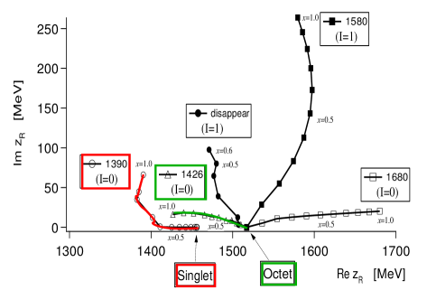
Figure 3: Trajectories of the poles in the scattering amplitudes obtained by changing the SU(3) breaking parameter $x$. In the SU(3) limit ($x=0$), only two poles appear, one for the singlet and the other for the octets. The symbols correspond to the step size $\delta x=0.1$ and the two trajectories contributing to the $\Lambda(1405)$ are high-lighted.

The location of the poles are: Pole 1 at $(1379.2-i27.6)~{}{\rm MeV}$ and pole 2 at $(1433.7-i11.0)~{}{\rm MeV}$ on sheet II, close to the $\pi\Sigma$ and $K^{-}p$ thresholds, respectively. This two-pole structure was also found in follow-up works by other groups [45, 46]. A better understanding of this two-pole structure was achieved in Ref. [47] using SU(3) symmetry considerations and group theory. For the case under consideration, namely the dynamical generation of resonances in Goldstone boson scattering off baryons, the following group theoretical consideration applies: The decomposition of the combination of the two octets, the Goldstone bosons and the ground-state baryons, is

$$8\otimes 8=\underbrace{1\oplus 8_{s}\oplus 8_{a}}_{\rm binding~{}at~{}LO}\oplus 10\oplus\overline{10}\oplus 27~{},$$ (18)

where using the leading order WT-term one finds poles in the singlet and in the two octets. The two octets are degenerate and the poles are located on the real axis, see Fig. 3. One can now follow the developments of these poles in the complex plane. For that, one parameterizes the departure from the SU(3) limit for the GB ($M_{i}$) and baryon masses ($m_{i}$) and subtraction constants $a_{i}$ (the subtraction constants can be channel-dependent but collapse to one value in the SU(3) limit) as follows:

$$M_{i}^{2}(x)=M_{0}^{2}+x(M_{i}^{2}-M_{0}^{2})~{},~{}~{}m_{i}(x)=m_{0}+x(m_{i}-m_{0})~{},~{}~{}a_{i}(x)=a_{0}+x(a_{i}-a_{0})~{},$$ (19)

with $0\leq x\leq 1$, where $x=0$ corresponds to the SU(3) limit and $x=1$ describes the physical world. Further, $m_{0}=1151\,$MeV, $M_{0}=368\,$MeV and $a_{0}=-2.148$. The trajectories of the various poles in the complex plane as the SU(3) breaking is gradually increased up to the physical values at $x=1$ is shown in Fig. 3. First, we observe that not all poles present in the SU(3) limit appear for $x=1$ (using the LO WT term only). Second, what concerns the $\Lambda(1405)$, we see that the singlet pole moves towards the $\pi\Sigma$ threshold and becomes rather broad, whereas the second pole from the octet comes out close to the $K^{-}p$ threshold and stays rather narrow. So there are in fact two resonances. Having determined these poles, one can determine the couplings of these resonances to the physical states by studying the amplitudes in the vicinity of the poles,

$$T_{ij}=\frac{g_{i}g_{j}}{z-z_{R}}+{\rm regular~{}terms}~{},$$ (20)

with $i,j$ channel indices and the couplings $g_{i}$ are complex valued numbers. While the lower pole couples stronger to the $\pi\Sigma$ channel, the higher one displays a stronger coupling to $\bar{K}N$. Consequently, it is possible to find the existence of the two resonances by performing different experiments, since in different experiments the weights by which the two resonances are excited are different, see Ref. [47] for more details. Further early support of the two-pole scenario was provided by the leading order investigation of the reaction $K^{-}p\to\pi^{0}\pi^{0}\Sigma^{0}$ [48].

3.4 Beyond leading order

Figure 4: 3-dimensional plot of the two-pole structure of the $\Lambda(1405)$. $W$ denotes the center-of-mass energy. Figure courtesy of Maxim Mai.

Clearly, to achieve a better precision, one has to go beyond leading order and include the next-to-leading order (NLO) terms in the chiral SU(3) Lagrangian in the effective potential. This task was performed by three groups independently [49, 50, 51]. These investigations were also triggered by the precise measurements of the energy shift and width of kaonic hydrogen [52], which was based on the improved Deser-type formula from Ref. [53], thus resolving the long standing “kaonic hydrogen puzzle” (the discrepancy between the values of the $\bar{K}N$ scattering lengths extracted from scattering data or earlier kaonic hydrogen experiments). This allowed to pin down the subthreshold $K^{-}p$ scattering amplitude to better precision and to make predictions for the $K^{-}n$ scattering lengths. Most importantly, all of these works confirmed the two-pole structure as shown in Fig. 4 from [51].

There was yet another surprise, namely by looking more closely at the scattering and kaonic hydrogen data, one can find at least eight solutions of similar quality with different pairs of poles for the $\Lambda(1405)$, see Ref. [54]. Here, photoproduction comes to the rescue. The CLAS collaboration at Jefferson Laboratory did a superb job in measuring the $\Sigma\pi$ photoproduction line shapes near the $\Lambda(1405)$ [55]. These data were first analyzed using LO unitarized CHPT and a polynomial ansatz for the photoproduction process $\gamma p\to K^{+}M_{i}B_{i}$ in Ref. [56], leading to a good fit of these data and a further check of the two-pole nature of the $\Lambda(1405)$. The same ansatz was used in [54], leaving only two of the eight solutions, as shown for one of the remaining solutions in Fig. 5 for a fraction of the data (the complete fit is shown in [54]). Similarly, the spread in the two poles from the eight solutions was sizeably reduced, although the lower pole could not be pinned down as well as the higher one. This work also supplied error bands, not only for the photoproduction results but also for the underlying hadronic scattering processes. This shows that the inclusion of the photoproduction data serves as a new important constraint on the antikaon-nucleon scattering amplitude. In view of all these NLO results, the two-pole structure first appeared in the RPP in form of a mini-review [57], called “Pole structure of the $\Lambda(1405)$ region” co-authored by Hyodo and Meißner, which give also references to other works related to the two-pole scenario. Still, in the RPP summary tables the $\Lambda(1405)$ was listed (and still is) as one resonance only.

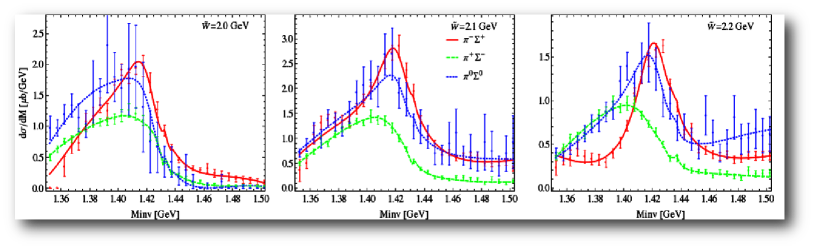
Figure 5: Result of the fits to the CLAS data in all three channels $\pi^{+}\Sigma^{-}$ (green), $\pi^{-}\Sigma^{+}$(red) and $\pi^{0}\Sigma^{0}$. Correspondingly, green (dashed), red (full) and blue (dotted) lines represent the outcome of the model for the solution 4 in the $\pi^{+}\Sigma^{-},\pi^{-}\Sigma^{+},\pi^{0}\Sigma^{0}$ channels, respectively. Figure courtesy of Maxim Mai.

3.5 Where do we stand?

Low-energy meson-baryon interactions in the strangeness $S=-1$ sector have been considered by a number of groups world-wide. A comparative study of various chiral unitary approaches was given in Ref. [58]. These approaches are based on a chiral Lagrangian that includes terms up to NLO, ${\cal O}(p^{2})$ [49, 50, 51, 59]. The various LECs (and others parameters) are determined from a fit to the low-energy $K^{-}p$ scattering data as well as to the properties of kaonic hydrogen measured by the SIDDHARTA collaboration. It was thus possible to not only compare the pole content of these various approaches but also the subthreshold energy dependence of the $\bar{K}N$ scattering amplitudes, which are important e.g. in the description of kaonic nuclei. These models differ in technical details but also in some underlying philosophical aspects. Largely, dimensional regularization is used to tame the ultraviolet divergences in the meson-baryon loop function and the meson-baryon interactions are considered on the energy shell. This holds for the Kyoto-Munich, Murcia and Bonn models. Differently from that, the Prague model introduces off-shell form factors to regularize the Green function and phenomenologically accounts for the off-shell effects. In all but one of these approaches an effective meson-baryon potential is introduced and matched to the chiral amplitude up to a given order. This potential is then iterated in a Lippmann-Schwinger equation to generate the bound and scattering states.

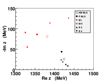
Figure 6: Pole positions for various approaches: Kyoto-Munich (KM) [49], Prag (P) [59], Murcia (M) [50] and Bonn (B) [51].

In case of the Bonn model, a Bethe-Salpeter equation is solved followed by an S-wave projection. Also, the off-shell contributions are neglected. Further, in the Kyoto-Munich and Prague approaches, the NLO corrections to the LO part are kept moderately small while in the Murcia and Bonn models sizable NLO terms are generated. These lead to inter-channel couplings very different from those obtained by only the WT interaction. Nevertheless, these different models reproduce the experimental data on a qualitatively very similar level. They are also in mutual agreement for the data available at the $\bar{K}N$ threshold and they agree on the position of the higher pole for the $\Lambda(1405)$ resonance. The predicted complex energy has a real part $\Re z\approx 1420\ldots 1430$ MeV and an imaginary part $-\textrm{Im}\,z\approx 10\ldots 40$ MeV, see Fig. 6. These different approaches, however, also lead to some distinct differences in their predictions. In particular, one finds very different locations of the lighter pole and different predictions for the elastic $K^{-}p$ and $K^{-}n$ amplitudes at sub-threshold energies. This certainly has impact on the predictions one can make (or has made) for kaonic atoms and antikaon quasi-bound states, see e.g. [60].

Clearly, we need better data to constrain the $\pi\Sigma$ spectra in various processes besides the already mentioned photoproduction data. A step in this direction was performed in Ref. [61]. These authors provide further constraints on the $\bar{K}N$ subthreshold interaction by analyzing $\pi\Sigma$ spectra in various processes, such as the $K^{-}d\to\pi\Sigma n$ reaction and the $\Lambda_{c}\to\pi\pi\Sigma$ decay. Also, the yet to be measured 1S level shift of kaonic deuterium will put further constraints on the $\bar{K}N$ interaction [63, 62]. For the status of such measurements, see [64]. Further progress has also been made by including the P-waves and performing a sophisticated error analysis [65], confirming again and sharpening further the two-pole scenario of the $\Lambda(1405)$ (note that the P-waves had already been included earlier with a focus on the $S=0$ sector [66]). Despite these remaining uncertainties, it must be stated clearly that the two-pole nature of the $\Lambda(1405)$ is established!

To end this section, I briefly discuss two recent works that challenged the two-pole structure. It was claimed in Ref. [67] that the two-pole nature is an artifact of the on-shell approximation used in most studies. Including off-shell effects, only one pole is generated in that study. However, as convincingly shown in Ref. [68], that approach violates constraints imposed by chiral symmetry. What is the origin of this violation? It is partly due to the treatment of the off-shell chiral-effective vertices, in combination with the employed regularization scheme and the use of the non-relativistic approximation. Overcoming these deficiencies, the two-pole scenario reappears. This does not come as a surprise as the NLO study of Ref. [51] already went beyond the on-shell approximation. Another recent paper with only one pole is Ref. [69], based on the phenomenological Bonn-Gatchina (BnGa) approach. In this framework, a large number of scattering and photoproduction data is fitted. However, this scheme does not allow for the dynamical generation of resonances and no pole searches in the complex-energy plane are reported in [69]. In a recent update, these authors also included a second pole in their model [70]. They find that the second pole does not considerably worsen the description of the considered data but still they prefer the solution with one pole. Thus, these results are not conclusive. In addition, data that further support the two-pole nature on $\pi^{-}p\to K^{0}\pi\Sigma$ and $pp\to pK^{+}\pi\Sigma$ [71] as well as $K^{+}\Lambda(1405)$ electroproduction [72] are also not included. It can therefore safely be said that these papers do indeed not challenge the two-pole scenario.

4 Meson sector: The $D_{0}^{*}(2300)$ and related states

So far, one might consider the two-pole structure a curiosity related to just one particular state. In the meson sector, a similar doubling of states was already considered in 1986 in the discussion of the mysterious decay properties of the $f_{0}(980)$ (then called $\delta(980)$), but that remained largely unnoticed [73]. However, let us now take a closer look at the spectrum of the excited charmed mesons, especially the $D_{s0}^{*}(2317)$ first observed by BaBar [74] and the $D_{0}^{*}(2300)$ first observed by Belle [75] (see also Ref. [76]). According to the recent edition of the PDG, the characteristics of these states are:

$$D_{0}^{*}(2300) : ~{}~{}M=2300\pm 19~{}{\rm MeV}~{},~{}~{}\Gamma=274\pm 40~{}{\rm MeV}~{},~{}~{}I(J^{P})=\frac{1}{2}(0^{+})~{},$$ (21)

$$D_{s0}^{*}(2317) : ~{}~{}M=2318.0\pm 0.7~{}{\rm MeV}~{},~{}~{}\Gamma<3.8~{}{\rm MeV}~{},~{}~{}I(J^{P})=0(0^{+})~{}.$$ (22)

According to the quark model, the quark composition for these scalar mesons is $c\bar{u}$ and $c\bar{s}$, respectively. This immediately poses the question: Why is the $D_{s0}^{*}(2317)$ as heavy as the $D_{0}^{*}(2300)$, it should be about 100 MeV, which is the mass of the strange quark, heavier? Also, why is the $D_{s0}^{*}(2317)$ about 150 MeV below the prediction of the quark model, that has been rather successful [3]? While this is an interesting question (I refer to the review [77] which has a very detailed discussion of this state), here I will focus on the the non-strange charmed scalar meson, as it appears to be too heavy, but in fact will give further support to the two-pole scenario.

4.1 Two-pole structure

Let us consider first the fine lattice QCD work by the Hadron Spectrum Collaboration, who investigated coupled-channel $D\pi$, $D\eta$ and $D_{s}\bar{K}$ scattering with $J^{P}=0^{+}$ and $I=1/2$ in three lattice volumes, one value for the temporal and the spatial lattice spacing, respectively, at a pion mass $M_{\pi}=391\,$MeV and $D$-meson mass $M_{D}=1885\,$MeV [78]. They used various $K$-matrix type extrapolations of the type

$$K_{ij}=\left(g_{i}^{(0)}+g_{i}^{(1)}s\right)\left(g_{j}^{(0)}+g_{j}^{(1)}s\right)\frac{1}{m^{2}-s}+\gamma_{ij}^{(0)}+\gamma_{ij}^{(1)}s~{},$$ (23)

to find the poles in the complex plane, by fitting the parameters $g,\gamma$ to the computed energy levels, and use the $T$-matrix to extract the poles. They found one S-wave pole at $(2275.0\pm 0.9)\,$MeV, extremely close to the $D\pi$ threshold at 2276 MeV. This state is consistent with the $D_{0}^{*}(2300)$ of the PDG. However, the extrapolations in Eq. (23) do not take into account chiral symmetry.

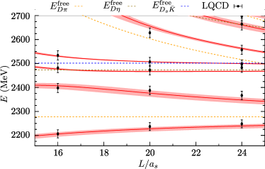
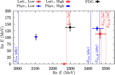
Figure 7: Left panel: Energy levels calculated in finite-volume unitarized chiral perturbation theory with all LECs determined before (red bands representing the 1$\sigma$ uncertainties) in comparison to the lattice QCD results of [78] (black circles). The dashed lines give the various free levels of the two-particle systems $D\pi$, $D\eta$ and $D_{s}\bar{K}$. Right panel: Location of the two poles in the complex energy plane for the lattice masses (red symbols) and physical masses (blue symbols). The black diamond represents the PDG value. The various thresholds are indicated by the dotted lines. Figures courtesy of Feng-Kun Guo.

Therefore, this topic was revisited in Ref. [79], where the chiral Lagrangian, Eq. (2.3), together with LECs from Ref. [26] was implemented within the finite volume formalism outlined in Sect. 2.5 to postdict in a parameter-free manner the energy levels measured by the Hadron Spectrum Collaboration. The stunning result of this unitarized CHPT calculation is shown in the left panel of Fig. 7, a very accurate postdiction of the lattice levels is achieved (note that this is not a fit). Note further that the region above 2.7 GeV is beyond the range of applicability of this NLO calculation. The level below the $D\pi$ threshold is interpreted in Ref. [78] as a bound state associated to the $D_{0}^{*}(2300)$ as stated before. The finite-volume UCHPT calculation also finds this pole at $M=2264_{-14}^{+8}\,$MeV and half-width $\Gamma/2=0\,$MeV, very similar to the results of Ref. [78]. However, there is a second pole at $M=2468_{-25}^{+32}\,$MeV with $\Gamma/2=113^{+18}_{-16}\,$MeV, see also the right panel of Fig. 7. Using chiral extrapolations, one can then evaluate the spectroscopic content of the scattering amplitudes for the physical pion mass, collected in Tab. 1.

Table 1: Position $\sqrt{s}=M-i\Gamma/2$ (in MeV) and couplings (in GeV) of the two poles in the (0,1/2) sector using physical pion masses.

$M$ (MeV)	$\Gamma/2$ (MeV)	$|g_{D\pi}|$	$|g_{D\eta}|$	$|g_{D_{s}\bar{K}}|$
$2105^{+6}_{-8}$	$102^{+10}_{-12}$	$9.4^{+0.2}_{-0.2}$	$1.8^{+0.7}_{-0.7}$	$4.4^{+0.5}_{-0.5}$
$2451^{+36}_{-26}$	$134^{+7}_{-8}$	$5.0^{+0.7}_{-0.4}$	$6.3^{+0.8}_{-0.5}$	$12.8^{+0.8}_{-0.6}$

The bound state below the $D\pi$ threshold evolves into a resonance above it when the physical masses are used, where the threshold is now at 2005 MeV. This behaviour is typical for S-wave poles. The second pole moves very little and its couplings are rather independent of the meson masses. It is a resonance located between the $D\eta$ and $D_{s}\bar{K}$ thresholds on the (110) Riemann sheet, continuously connected to the phyical sheet. Thus, the $D_{0}^{*}(2300)$ of the RPP is produced by two different poles, and in fact the lower pole solves the enigma discussed in the beginning of this section. Note that this two-pole structure was observed earlier in Refs. [80, 81, 82] but only explained properly in  [79] as discussed next.

Consider again the SU(3) limit, where the eight Goldstone bosons take the common value $M_{0}$ and the three heavy $D$-mesons the common value $M_{D0}$, so that departures from the SU(3) limit are parameterized as

$$M_{\phi,i} = M_{\phi,i}^{\rm phys}+x(M_{0}-M_{\phi,i}^{\rm phys})~{}(i=1,\ldots 8)~{},$$

$$M_{D,j} = M_{D,j}^{\rm phys}+x(M_{D0}-M_{D,j}^{\rm phys})~{}(j=1,\ldots 3)~{},$$

with $x=0$ and $x=1$ corresponding to the physical and the SU(3) symmetric case, respectively, and $M_{0}=0.49\,$ GeV and $M_{D0}=1.95\,$GeV. In that study, only one subtraction constant for all channels was used and kept fixed with varying $x$. Note that in contrast to the work of Ref. [47] discussed before, here a linear extrapolation formula is used for the GB masses, which is also legitimate. As before, the two-pole nature is understood from group theory,

$$\bar{3}\otimes 8=\underbrace{\bar{3}\oplus 6}_{\rm attractive}\oplus\overline{15}~{}.$$ (24)

This means one has attraction in the $\bar{3}$ and $6$ irreducible representations (irreps) but repulsion in the $\overline{15}$ irrep at leading order in the effective potential. The most attractive irrep, the $\bar{3}$, admits a $c\bar{q}$ ($q=u,d,s$) configuration. At NLO, the potentials receive corrections, but the qualitative features remain. The evolution from the SU(3) limit to the physical case is shown in the left panel of Fig. 8. Shown are the two poles corresponding to the $D_{0}^{*}(2300)$ and its strange sibling, the $D_{s0}^{*}(2317)$. As one moves away from the SU(3) limit, the lower pole of the $D_{0}^{*}(2300)$ moves down in the complex plane, restoring the expected ordering that the $c\bar{u}$ excitation should be lighter than its $c\bar{s}$ partner.

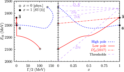
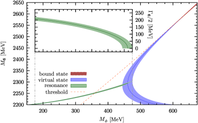
Figure 8: Left panel: Pole paths in the complex plane when recovering the SU(3) limit (left subpanel). Mass evolution of the different poles with $x$. Besides the two (0,1/2) poles, denoted as high and low (blue dashed and green solid lines), the evolution of the (1,0) bound state, the $D_{s0}^{*}(2317)$ resonance (orange dot-dashed line), is shown (right subpanel). Figure courtesy of Feng-Kun Guo. Right panel: Mass of the predicted sextet state $M_{6}$ at the SU(3) symmetric point as a function of the Goldstone boson mass $M_{\phi}$. The inset shows the half-width of the resonance for GB masses below 475 MeV.

It was already observed in Ref. [79] that the higher pole connects with a virtual state in the sextet representation due to the weaker binding. This issue was further elaborated on in Ref. [83], where the SU(3) limit was studied in more detail. In the right panel of Fig. 8 the sextet pole is shown for varying GB masses. Below $M_{\phi}\lesssim 475$ MeV, the pole is a resonance with its imaginary part ($\Gamma_{\bm{6}}/2$) shown in the inserted sub-figure. Above $M_{\phi}\simeq 475$ MeV, it evolves into a pair of virtual states, and finally it becomes a bound state at $M_{\phi}\simeq 600$ MeV. Such a study in the SU(3) limit $m_{u}=m_{d}=m_{s}$ at large GB masses could be performed on the lattice and offer another test of this scenario. Finally, let me come back to the lattice calculation of Ref. [78]. Indeed, while various of the amplitudes employed in that analysis contained a second pole, its location was strongly parameterization-dependent [84], and therefore not reported in that paper.

4.2 Other candidates

As already noted, in the $(S,I)=(1,0)$ sector, the same chiral Lagrangian produces a pole at $2315^{+18}_{-28}$ MeV which is naturally identified with the $D_{s0}^{*}(2317)$. It emerges from the pole in the triplet representation. The $D_{s0}^{*}(2317)$ is dominantly a $DK$ molecule. Substituting the $D$-meson by a $D^{*}$ and employing HQSS, the molecular picture naturally gives [85]

$$M_{D_{s1}(2460)}-M_{D_{s0}^{*}(2317)}\simeq M_{D^{*}}-M_{D}~{},$$ (25)

which is also obtained in the so-called doublet model [86, 87, 88]. Similar to the $D_{0}^{*}(2300)$, the nonstrange charmed meson $D_{1}$ also comes with two poles, see Tab. 2. This was noted before in [89]. In both cases the single RPP pole sits in between the lower and the higher pole.

Using HQFS, one can further predict similar states in the $B$-meson sector, by just replacing the corresponding $D$-mesons with their bottom counterparts at leading order [81, 85]. Using the NLO framework employed in the charm sector, one has to scale the LECs $h_{0,1,2,3}\sim m_{Q}$ and $h_{4,5}\sim 1/m_{Q}$ and the subtraction constant is adjusted as described in Ref.  [81]. This leads again to the two-pole structures also collected in Tab. 2.

For the lowest positive-parity heavy strange mesons, it is instructive to compare with lattice QCD results. This gives for the masses of the charm-strange mesons $M_{D_{s0}^{*}}=2315^{+18}_{-28}[2348^{+7}_{-4}]$ [90] , $M_{D_{s1}}=2456^{+15}_{-21}[2459.5\pm 0.6]$ [90] , and for the strange-bottom ones $M_{B_{s0}^{*}}=5720^{+16}_{-23}[5711\pm 23]$ [91] , $M_{D_{s1}}=5772^{+15}_{-21}[5750\pm 25]$ [91] , where the first [second] number refers to the molecular [lattice QCD] prediction. The agreement is rather remarkable.

Table 2: Predicted poles corresponding to the positive-parity heavy-light nonstrange mesons given as ($M,\Gamma/2$), with $M$ the mass and $\Gamma$ the total decay width, in units of MeV. The current RPP [4] values are listed in the last column.

	lower pole	higher pole	RPP
$D_{0}^{*}$	$\left(2105^{+6}_{-8},102^{+10}_{-11}\right)$	$\left(2451^{+35}_{-26},134^{+7}_{-8}\right)$	$(2300\pm 19,137\pm 20)$
$D_{1}$	$\left(2247^{+5}_{-6},107^{+11}_{-10}\right)$	$\left(2555^{+47}_{-30},203^{+8}_{-9}\right)$	$(2427\pm 26\pm 25,192^{+54}_{-38}\pm 37)$
$B_{0}^{*}$	$\left(5535^{+9}_{-11},113^{+15}_{-17}\right)$	$\left(5852^{+16}_{-19},36\pm 5\right)$	-
$B_{1}$	$\left(5584^{+9}_{-11},119^{+14}_{-17}\right)$	$\left(5912^{+15}_{-18},42^{+5}_{-4}\right)$	-

So the plot of the two-pole scenario thickens. In the absence of direct measurements of some of these states, one might ask the question whether there is further experimental support for the picture just outlined?

4.3 Analysis of $B\to D\pi\pi$ data

To further test the mechanism of the dynamical generation of the charm-light flavored mesons discussed so far, let me turn to the high precision results of the LHCb collaboration for the decays $B\to D\pi\pi$ [92]. As shown in Ref. [83], the amplitudes with the two $D_{0}^{*}$ states are fully consistent with the LHCb measurements of the reaction $B^{-}\to D^{+}\pi^{-}\pi^{-}$, which are at present the best data providing access to the $D\pi$ system and thus to the nonstrange scalar charm mesons. This information is encoded in the so-called angular momenta, which are discussed in detail in the LHCb paper [92].

The theoretical framework to analyse this process is based on the unitarized chiral effective Lagrangian, Eq. (10), where one pion is fast and the other participates in the $D\pi$ final-state interactions (for more details, see Ref. [83]). To be specific, consider the reaction $B^{-}\to D^{+}\pi^{-}\pi^{-}$. For sufficiently low energies in the $D\pi$ system, it suffices to include the lowest partial waves (S,P,D), so we can write the decay amplitude as

$${\cal{A}}(B^{-}\to D^{+}\pi^{-}\pi^{-})=\sum_{L=0}^{2}\sqrt{2L+1}{\cal{A}}_{L}(s)P_{L}(z)\,,$$ (26)

where ${\cal{A}}_{0,1,2}(s)$ correspond to the amplitudes with $D^{+}\pi^{-}$ in the S- , P- and D-waves, respectively, and $P_{L}(z)$ are the Legendre polynomials. For the P- and D-wave amplitudes we use the same Breit-Wigner form as in the LHCb analysis [92], containing the $D^{*}$ and $D^{*}(2680)$ mesons in the P-wave and the $D_{2}(2460)$ in the D-wave. For the S-wave, however, we employ

$${\cal{A}}_{0}(s) = A\bigg{\{}E_{\pi}\!\left[2+G_{1}(s)\left(\frac{5}{3}T^{1/2}_{11}(s)+\frac{1}{3}T^{3/2}(s)\right)\right]$$ (27)

$$+\frac{1}{3}E_{\eta}G_{2}(s)T^{1/2}_{21}(s)+\sqrt{\frac{2}{3}}E_{\bar{K}}G_{3}(s)T^{1/2}_{31}(s)\bigg{\}}+BE_{\eta}G_{2}(s)T^{1/2}_{21}~{},$$

where $A$ and $B$ are two independent couplings following from SU(3) flavor symmetry (i.e. combinations of the LECs $c_{i}$, $A=\sqrt{2}(c_{1}+c_{4})/F_{\phi}$ and $B=2\sqrt{2}(c_{2}+c_{6})/(3F_{\phi})$, with $F_{\phi}$ the GB decay constant), and $E_{\pi,\eta,\bar{K}}$ are the energies of the light mesons. Further, the $T^{I}_{ij}(s)$ are the S-wave scattering amplitudes for the coupled-channel system with total isospin $I$, where $i,j$ are channel indices with $1,2$ and $3$ referring to $D\pi$, $D\eta$ and $D_{s}\bar{K}$, respectively, and the $G_{i}(s)$ are the corresponding 2-point loop functions. These scattering amplitudes are again taken from Ref. [26] where also all the other parameters were fixed. To filter out the S-wave, the following (combinations of) angular moments are used:

$$\langle P_{0}\rangle \propto |{\mathcal{A}}_{0}|^{2}+|{\mathcal{A}}_{1}|^{2}+|{\mathcal{A}}_{2}|^{2}~{},$$

$$\langle P_{2}\rangle \propto \frac{2}{5}|{\mathcal{A}}_{1}|^{2}+\frac{2}{7}|{\mathcal{A}}_{2}|^{2}+\frac{2}{\sqrt{5}}|{\mathcal{A}}_{0}||{\mathcal{A}}_{2}|\cos(\delta_{2}-\delta_{0})~{},$$

$$\langle P_{13}\rangle = \langle P_{1}\rangle-\frac{14}{9}\langle P_{3}\rangle\propto\frac{2}{\sqrt{3}}|{\mathcal{A}}_{0}||{\mathcal{A}}_{1}|\cos(\delta_{1}-\delta_{0})~{},$$ (28)

with $\delta_{0},\delta_{1},\delta_{2}$ the S-, P-, D-wave phase shift, respectively.

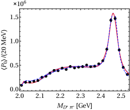
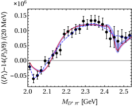
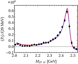
Figure 9: Fit to the LHCb data for the angular moments $\langle P_{0}\rangle$, $\langle P_{13}\rangle$ and $\langle P_{2}\rangle$ for the $B^{-}\to D^{+}\pi^{-}\pi^{-}$ reaction [92]. The largest error among $\langle P_{1}\rangle$ and $14\langle P_{3}\rangle/9$ in each bin is taken as the error of $\langle P_{1}\rangle-14\langle P_{3}\rangle/9$. The solid lines show the results of [83], with error bands corresponding to the one-sigma uncertainties propagated from the input scattering amplitudes, while the dashed lines stand for the LHCb fit using cubic splines for the S-wave [92].

The best fit to the LHCb data is shown in Fig. 9 together with their best fit provided by LHCb based on cubic splines (dashed lines). The bands in Fig. 9 reflect the one-sigma errors of the parameters in the scattering amplitudes determined in Ref. [26]. It is worthwhile to notice that in $\langle P_{13}\rangle$, where the $D_{2}(2460)$ does not play any role, the data show a significant variation between 2.4 and 2.5 GeV. Theoretically this feature can now be understood as a signal for the opening of the $D^{0}\eta$ and $D_{s}^{+}K^{-}$ thresholds at 2.413 and 2.462 GeV, respectively, which leads to two cusps in the amplitude. This effect is amplified by the higher pole which is relatively close to the $D_{s}\bar{K}$ threshold on the unphysical sheet. There is some discrepancy between the chiral amplitude and the data for $\langle P_{13}\rangle$ at low energies: Does this point at a deficit of the former? Fortunately the LHCb Collaboration provided more detailed information on their S-wave amplitude in Ref. [92]: In the analysis of the data a series of anchor points were defined where the strength and the phase of the S-wave amplitude were extracted from the data. Then cubic splines were used to interpolate between these anchor points.

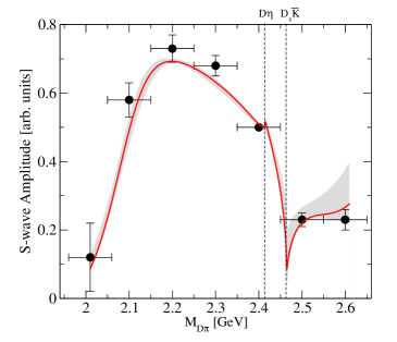
Figure 10: Comparison of the S-wave amplitude based on UCHPT to the S-wave anchor points found in the experimental analysis, shown as the data points [92]. The red line gives the best fit results and the grey band quantifies the uncertainties that emerged from the fitting procedure. The fitting range extends up to 2.55 GeV. The dashed perpendicular lines indicate the location of the $D\eta$ and $D_{s}\bar{K}$ threshold, respectively.

In Fig. 10 the S-amplitude fixed as described above is compared to the LHCb anchor points. Not only shows this figure very clearly that the strength of the S-wave amplitude largely determined by the fits to lattice data is fully consistent with the one extracted from the data for $B^{-}\to D^{+}\pi^{-}\pi^{-}$, the shown amplitude also shows the importance of the $D\eta$ and $D_{s}\bar{K}$ cusps and thus also of the role of the higher pole in the $I=1/2$ and $S=0$ channel even more clearly than the angular moments discussed above. This clearly highlights the importance of a coupled-channel treatment for this reaction. An updated analysis of the LHC Run-2 data is called for to confirm the prominence of the two cusps.

LHCb presented also data on $B_{s}^{0}\to\bar{D}^{0}K^{-}\pi^{+}$, which are, however, less precise than the ones just discussed. Using the same formalism as before, with one different combination of the LECs $c_{i}$ and the same resonances in the P- and D-wave as LHCb, these data can be well described by a one parameter fit, see Ref. [83] for more details. A combined analysis including also data for $B^{0}\to\bar{D}^{0}\pi^{-}\pi^{+}$, $B^{-}\to D^{+}\pi^{-}K^{-}$ and $B_{s}^{0}\to\bar{D}^{0}K^{-}\pi^{+}$ performed in Ref. [93] gives further credit to this picture.

4.4 The $K_{1}$ meson

Another state that offered support to the two-pole scenario even before the heavy-light mesons just discussed is the axial-vector meson $K_{1}(1270)$, which in the quark model is a kaonic excitation with angular momentum one, $I(J^{P})=\frac{1}{2}(1^{+})$. The two-pole nature of the $K_{1}(1270)$ was first noted in the study of the scattering of vector mesons off the Goldstone bosons in a chiral unitary approach at tree level [94]. This was further sharpened in Ref. [95]. There, the high-statistics data from the WA3 experiment on $K^{-}p\to K^{-}\pi^{+}\pi^{-}p$, analyzed by the ACCMOR collaboration [96], were reanalyzed and shown to favor a two-pole interpretation of the $K_{1}(1270)$. The authors of Ref. [95] also reanalyzed the traditional K-matrix interpretation of the WA3 data and found that the good fit of the data obtained there was due to large cancellations of terms of unclear physical interpretation. It was recently shown how this two-pole scenario can show up in $D$-meson decays, in particular $D^{0}\to\pi^{+}VP$ and $D^{+}\to\nu e^{+}VP$, where $P$ and $V$ are pseudoscalar and vector mesons, respectively [97, 98].

5 Discussion and Outlook

Let me summarize briefly:

• The story with the two-pole structure started with the $\Lambda(1405)$, which can now be considered as established. Still, the position of lighter pole close to the $\pi\Sigma$ threshold needs to be determined better whereas the higher pole close to the $K^{-}p$ threshold is pretty well pinned down. It is comforting to note that the re-analysis of the Jülich $\bar{K}N$ meson-exchange model from the 1990s also confirmed the two-pole structure of the $\Lambda(1405)$, see Ref. [99] (and references therein). I again point out that approaches, that do not allow for the dynamical generation of resonances, like e.g. the BnGa model, are insufficient for describing the whole hadron spectrum.

• Further support of the two-pole scenario comes from charmed baryons. Recently, an analysis of the LHCb data on $\Lambda_{b}\to pD^{0}\pi^{-}$ in the near-$pD^{0}$-threshold region also revealed a two-pole structure of the $\Sigma_{c}(2800)^{+}$ when isospin-breaking is taken into account [100].

• The spectrum of excited charmed mesons, made from a heavy $c$ quark and a light $u,d,s$ quark, offers further support of the two-pole structure and the dynamical generation of hadron resonances. Here, a beautiful interplay of experimental results, unitarized chiral perturbation theory and lattice QCD gives very strong indications that this picture is indeed correct. Further lattice calculations and the measurement of the corresponding $B$-mesons will serve as further tests.

• This leads to a new paradigm in hadron physics: The hadron spectrum must not be viewed as a collection of quark model states, but rather as a manifestation of a more complex dynamics that leads to an intricate pattern of various types of states that can only be understood by an interplay of theory and experiment (cf. the light scalar mesons or the states discussed here).

• The dynamical generation of hadron states through hadron-hadron interactions ties together nuclear and particle physics, as these molecular compounds bear resemblance to the light nuclei, the deuteron, the triton and so on. Therefore, such molecular states were called “deusons” by Törnquist, one of the pioneers in the field of hadronic molecules [101].

From all this, it is rather obvious that the PDG tables published in the RPP must undergo a drastic change and finally acknowledge the two-pole structure in the main listings, not just in the review section. Time will tell how long this necessary change will take.

References

- [1] M. Gell-Mann, “A Schematic Model of Baryons and Mesons,” Phys. Lett. 8 (1964) 214.
- [2] G. Zweig, “An SU(3) model for strong interaction symmetry and its breaking. Version 1,” CERN-TH-401 (1964).
- [3] S. Godfrey and N. Isgur, “Mesons in a Relativized Quark Model with Chromodynamics,” Phys. Rev. D 32 (1985) 189
- [4] M. Tanabashi et al. [Particle Data Group], “Review of Particle Physics,” Phys. Rev. D 98 (2018) no.3, 030001.
- [5] M. Neubert, “Heavy quark symmetry,” Phys. Rept. 245 (1994) 259. [hep-ph/9306320].
- [6] A. V. Manohar and M. B. Wise, “Heavy quark physics,” Camb. Monogr. Part. Phys. Nucl. Phys. Cosmol. 10 (2000) 1.
- [7] G. Burdman and J. F. Donoghue, “Union of chiral and heavy quark symmetries,” Phys. Lett. B 280 (1992) 287.
- [8] M. B. Wise, “Chiral perturbation theory for hadrons containing a heavy quark,” Phys. Rev. D 45 (1992) R2188.
- [9] T. M. Yan, H. Y. Cheng, C. Y. Cheung, G. L. Lin, Y. C. Lin and H. L. Yu, “Heavy quark symmetry and chiral dynamics,” Phys. Rev. D 46 (1992) 1148 Erratum: [Phys. Rev. D 55 (1997) 5851].
- [10] J. Gasser and H. Leutwyler, “Chiral Perturbation Theory to One Loop,” Annals Phys. 158 (1984) 142.
- [11] S. Weinberg, “Phenomenological Lagrangians,” Physica A 96 (1979) 327.
- [12] G. Ecker, “Chiral perturbation theory,” Prog. Part. Nucl. Phys. 35 (1995) 1 [hep-ph/9501357].
- [13] A. Pich, “Chiral perturbation theory,” Rept. Prog. Phys. 58 (1995) 563 [hep-ph/9502366].
- [14] V. Bernard and U.-G. Meißner, “Chiral perturbation theory,” Ann. Rev. Nucl. Part. Sci. 57 (2007) 33 [hep-ph/0611231].
- [15] J. Gasser and U.-G. Meißner, “Chiral expansion of pion form-factors beyond one loop,” Nucl. Phys. B 357 (1991) 90.
- [16] E. E. Jenkins and A. V. Manohar, “Baryon chiral perturbation theory using a heavy fermion Lagrangian,” Phys. Lett. B 255 (1991) 558.
- [17] V. Bernard, N. Kaiser, J. Kambor and U.-G. Meißner, “Chiral structure of the nucleon,” Nucl. Phys. B 388 (1992) 315.
- [18] T. Becher and H. Leutwyler, “Baryon chiral perturbation theory in manifestly Lorentz invariant form,” Eur. Phys. J. C 9 (1999) 643.
- [19] T. Fuchs, J. Gegelia, G. Japaridze and S. Scherer, “Renormalization of relativistic baryon chiral perturbation theory and power counting,” Phys. Rev. D 68 (2003) 056005.
- [20] V. Bernard, N. Kaiser and U.-G. Meißner, “Chiral dynamics in nucleons and nuclei,” Int. J. Mod. Phys. E 4 (1995) 193 [hep-ph/9501384].
- [21] V. Bernard, “Chiral Perturbation Theory and Baryon Properties,” Prog. Part. Nucl. Phys. 60 (2008) 82. [arXiv:0706.0312 [hep-ph]].
- [22] S. Scherer and M. R. Schindler, “Chiral perturbation theory for baryons,” Lect. Notes Phys. 830 (2012) 145.
- [23] H. Cheng, C. Cheung, G. Lin, Y. Lin, T. Yan and H. Yu, “Corrections to chiral dynamics of heavy hadrons: SU(3) symmetry breaking,” Phys. Rev. D 49 (1994), 5857-5881 [arXiv:hep-ph/9312304 [hep-ph]].
- [24] M. F. Lutz and M. Soyeur, “Radiative and isospin-violating decays of -mesons in the hadrogenesis conjecture,” Nucl. Phys. A 813 (2008), 14-95 [arXiv:0710.1545 [hep-ph]].
- [25] F. K. Guo, C. Hanhart, S. Krewald and U.-G. Meißner, “Subleading contributions to the width of the D*(s0)(2317),” Phys. Lett. B 666 (2008) 251 [arXiv:0806.3374 [hep-ph]].
- [26] L. Liu, K. Orginos, F. K. Guo, C. Hanhart and U.-G. Meißner, “Interactions of charmed mesons with light pseudoscalar mesons from lattice QCD and implications on the nature of the ,” Phys. Rev. D 87 (2013) no.1, 014508 [arXiv:1208.4535 [hep-lat]].
- [27] M. J. Savage and M. B. Wise, “SU(3) Predictions for Nonleptonic B Meson Decays,” Phys. Rev. D 39 (1989) 3346 Erratum: [Phys. Rev. D 40 (1989) 3127].
- [28] A. Dobado, M. J. Herrero and T. N. Truong, “Unitarized Chiral Perturbation Theory for Elastic Pion-Pion Scattering,” Phys. Lett. B 235 (1990) 134.
- [29] M. Döring, U.-G. Meißner, E. Oset and A. Rusetsky, “Unitarized Chiral Perturbation Theory in a finite volume: Scalar meson sector,” Eur. Phys. J. A 47 (2011) 139 [arXiv:1107.3988 [hep-lat]].
- [30] J. Gasser and H. Leutwyler, “Spontaneously Broken Symmetries: Effective Lagrangians at Finite Volume,” Nucl. Phys. B 307 (1988) 763.
- [31] R. H. Dalitz and S. F. Tuan, “A possible resonant state in pion-hyperon scattering,” Phys. Rev. Lett. 2 (1959) 425.
- [32] J. K. Kim, “Low Energy K- p Interaction of the 1405 MeV Resonance as KbarN Bound State,” Phys. Rev. Lett. 14 (1965) 29.
- [33] R. J. Hemingway, “Production of in Reactions at 4.2-GeV/,” Nucl. Phys. B 253 (1985) 742.
- [34] K. Moriya et al. [CLAS Collaboration], “Spin and parity measurement of the baryon,” Phys. Rev. Lett. 112 (2014) 082004 [arXiv:1402.2296 [hep-ex]].
- [35] P. J. Fink, Jr., G. He, R. H. Landau and J. W. Schnick, “Bound States, Resonances and Poles in Low-energy Interaction Models,” Phys. Rev. C 41 (1990) 2720.
- [36] N. Kaiser, P. B. Siegel and W. Weise, “Chiral dynamics and the low-energy kaon - nucleon interaction,” Nucl. Phys. A 594 (1995) 325 [nucl-th/9505043].
- [37] N. Kaiser, T. Waas and W. Weise, “SU(3) chiral dynamics with coupled channels: Eta and kaon photoproduction,” Nucl. Phys. A 612 (1997) 297 [hep-ph/9607459].
- [38] E. Oset and A. Ramos, “Nonperturbative chiral approach to s wave interactions,” Nucl. Phys. A 635 (1998) 99 [nucl-th/9711022].
- [39] J. A. Oller, E. Oset and A. Ramos, “Chiral unitary approach to meson meson and meson - baryon interactions and nuclear applications,” Prog. Part. Nucl. Phys. 45 (2000) 157 [hep-ph/0002193].
- [40] J. Oller, “Coupled-channel approach in hadron-hadron scattering,” Prog. Part. Nucl. Phys. 110 (2020) 103728 [arXiv:1909.00370 [hep-ph]].
- [41] J. Nacher, E. Oset, H. Toki and A. Ramos, “Radiative production of the Lambda(1405) resonance in K- collisions on protons and nuclei,” Phys. Lett. B 461 (1999) 299 [arXiv:nucl-th/9902071 [nucl-th]].
- [42] B. Borasoy, P. C. Bruns, U.-G. Meißner and R. Nissler, “Gauge invariance in two-particle scattering,” Phys. Rev. C 72 (2005) 065201 [hep-ph/0508307].
- [43] B. Borasoy, P. Bruns, U.-G. Meißner and R. Nissler, “A Gauge invariant chiral unitary framework for kaon photo- and electroproduction on the proton,” Eur. Phys. J. A 34 (2007) 161 [arXiv:0709.3181 [nucl-th]].
- [44] J. A. Oller and U.-G. Meißner, “Chiral dynamics in the presence of bound states: Kaon nucleon interactions revisited,” Phys. Lett. B 500 (2001) 263 [hep-ph/0011146].
- [45] D. Jido, A. Hosaka, J. C. Nacher, E. Oset and A. Ramos, “Magnetic moments of the and resonances,” Phys. Rev. C 66 (2002) 025203 [hep-ph/0203248].
- [46] C. Garcia-Recio, J. Nieves, E. Ruiz Arriola and M. J. Vicente Vacas, “S = -1 meson baryon unitarized coupled channel chiral perturbation theory and the S(01) Lambda(1405) and Lambda(1670) resonances,” Phys. Rev. D 67 (2003) 076009 [hep-ph/0210311].
- [47] D. Jido, J. A. Oller, E. Oset, A. Ramos and U.-G. Meißner, “Chiral dynamics of the two states,” Nucl. Phys. A 725 (2003) 181 [nucl-th/0303062].
- [48] V. Magas, E. Oset and A. Ramos, “Evidence for the two pole structure of the Lambda(1405) resonance,” Phys. Rev. Lett. 95 (2005) 052301 [arXiv:hep-ph/0503043 [hep-ph]].
- [49] Y. Ikeda, T. Hyodo and W. Weise, “Chiral SU(3) theory of antikaon-nucleon interactions with improved threshold constraints,” Nucl. Phys. A 881 (2012) 98 [arXiv:1201.6549 [nucl-th]].
- [50] Z. H. Guo and J. A. Oller, “Meson-baryon reactions with strangeness -1 within a chiral framework,” Phys. Rev. C 87 (2013) no.3, 035202 [arXiv:1210.3485 [hep-ph]].
- [51] M. Mai and U.-G. Meißner, “New insights into antikaon-nucleon scattering and the structure of the Lambda(1405),” Nucl. Phys. A 900 (2013) 51 [arXiv:1202.2030 [nucl-th]].
- [52] M. Bazzi et al. [SIDDHARTA Collaboration], “A New Measurement of Kaonic Hydrogen X-rays,” Phys. Lett. B 704 (2011) 113 [arXiv:1105.3090 [nucl-ex]].
- [53] U.-G. Meißner, U. Raha and A. Rusetsky, “Spectrum and decays of kaonic hydrogen,” Eur. Phys. J. C 35 (2004) 349 [hep-ph/0402261].
- [54] M. Mai and U.-G. Meißner, “Constraints on the chiral unitary amplitude from photoproduction data,” Eur. Phys. J. A 51 (2015) 30 [arXiv:1411.7884 [hep-ph]].
- [55] K. Moriya et al. [CLAS Collaboration], “Measurement of the photoproduction line shapes near the ,” Phys. Rev. C 87 (2013) no.3, 035206 [arXiv:1301.5000 [nucl-ex]].
- [56] L. Roca and E. Oset, “ poles obtained from photoproduction data,” Phys. Rev. C 87 (2013) no.5, 055201 [arXiv:1301.5741 [nucl-th]].
- [57] C. Patrignani et al. [Particle Data Group], “Review of Particle Physics,” Chin. Phys. C 40 (2016) no.10, 100001.
- [58] A. Cieply, M. Mai, U.-G. Meißner and J. Smejkal, “On the pole content of coupled channels chiral approaches used for the system,” Nucl. Phys. A 954 (2016) 17 [arXiv:1603.02531 [hep-ph]].
- [59] A. Cieply and J. Smejkal, “Chirally motivated amplitudes for in-medium applications,” Nucl. Phys. A 881 (2012) 115 [arXiv:1112.0917 [nucl-th]].
- [60] J. Mares, N. Barnea, A. Cieply, E. Friedman, A. Gal and D. Gazda, “Calculations of -nuclear quasi-bound states using chiral amplitudes,” EPJ Web Conf. 66 (2014) 09012.
- [61] Y. Kamiya, K. Miyahara, S. Ohnishi, Y. Ikeda, T. Hyodo, E. Oset and W. Weise, “Antikaon-nucleon interaction and (1405) in chiral SU(3) dynamics,” Nucl. Phys. A 954 (2016) 41 [arXiv:1602.08852 [hep-ph]].
- [62] T. Hoshino, S. Ohnishi, W. Horiuchi, T. Hyodo and W. Weise, “Constraining the interaction from the level shift of kaonic deuterium,” Phys. Rev. C 96 (2017) no.4, 045204 [arXiv:1705.06857 [nucl-th]].
- [63] U.-G. Meißner, U. Raha and A. Rusetsky, “Kaon-nucleon scattering lengths from kaonic deuterium experiments,” Eur. Phys. J. C 47 (2006) 473 [nucl-th/0603029].
- [64] C. Curceanu et al., “Kaonic Atoms to Investigate Global Symmetry Breaking,” Symmetry 12 (2020) no.4, 547.
- [65] D. Sadasivan, M. Mai and M. Döring, “S- and p-wave structure of meson-baryon scattering in the resonance region,” Phys. Lett. B 789 (2019) 329 [arXiv:1805.04534 [nucl-th]].
- [66] J. Caro Ramon, N. Kaiser, S. Wetzel and W. Weise, “Chiral SU(3) dynamics with coupled channels: Inclusion of P wave multipoles,” Nucl. Phys. A 672 (2000) 249 [nucl-th/9912053].
- [67] J. Revai, “Are the chiral based potentials really energy dependent?,” Few Body Syst. 59 (2018) 49 [arXiv:1711.04098 [nucl-th]].
- [68] P. C. Bruns and A. Cieply, “Importance of chiral constraints for the pole content of the scattering amplitude,” Nucl. Phys. A 996 (2020) 121702 [arXiv:1911.09593 [nucl-th]].
- [69] A. V. Anisovich, A. V. Sarantsev, V. A. Nikonov, V. Burkert, R. A. Schumacher, U. Thoma and E. Klempt, “Hyperon I: Study of the ,” arXiv:1905.05456 [nucl-ex].
- [70] A. V. Anisovich, A. V. Sarantsev, V. A. Nikonov, V. Burkert, R. A. Schumacher, U. Thoma and E. Klempt, “Hyperon III: coupled-channel dynamics in the mass region,” Eur. Phys. J. A 56 (2020) 139.
- [71] M. Bayar, R. Pavao, S. Sakai and E. Oset, “Role of the triangle singularity in production in the and processes,” Phys. Rev. C 97 (2018) no.3, 035203 [arXiv:1710.03964 [hep-ph]].
- [72] H. Y. Lu et al. [CLAS Collaboration], “First Observation of the Line Shape in Electroproduction,” Phys. Rev. C 88 (2013) 045202 [arXiv:1307.4411 [nucl-ex]].
- [73] R. Cahn and P. Landshoff, “Mystery of the Delta (980),” Nucl. Phys. B 266 (1986) 451.
- [74] B. Aubert et al. [BaBar], “Observation of a narrow meson decaying to at a mass of 2.32-GeV/c2,” Phys. Rev. Lett. 90 (2003) 242001 [arXiv:hep-ex/0304021 [hep-ex]].
- [75] K. Abe et al. [Belle], “Study of decays,” Phys. Rev. D 69 (2004), 112002 [arXiv:hep-ex/0307021 [hep-ex]].
- [76] J. Link et al. [FOCUS], “Measurement of masses and widths of excited charm mesons D(2)* and evidence for broad states,” Phys. Lett. B 586 (2004), 11-20 [arXiv:hep-ex/0312060 [hep-ex]].
- [77] F. Guo, C. Hanhart, U.-G. Meißner, Q. Wang, Q. Zhao and B. Zou, “Hadronic molecules,” Rev. Mod. Phys. 90 (2018) no.1, 015004 [arXiv:1705.00141 [hep-ph]].
- [78] G. Moir, M. Peardon, S. M. Ryan, C. E. Thomas and D. J. Wilson, “Coupled-Channel , and Scattering from Lattice QCD,” JHEP 10 (2016), 011 [arXiv:1607.07093 [hep-lat]].
- [79] M. Albaladejo, P. Fernandez-Soler, F. Guo and J. Nieves, “Two-pole structure of the ,” Phys. Lett. B 767 (2017), 465-469 [arXiv:1610.06727 [hep-ph]].
- [80] E. Kolomeitsev and M. Lutz, “On Heavy light meson resonances and chiral symmetry,” Phys. Lett. B 582 (2004) 39 [arXiv:hep-ph/0307133 [hep-ph]].
- [81] F. Guo, P. Shen, H. Chiang, R. Ping and B. Zou, “Dynamically generated 0+ heavy mesons in a heavy chiral unitary approach,” Phys. Lett. B 641 (2006) 285 [arXiv:hep-ph/0603072 [hep-ph]].
- [82] F. Guo, C. Hanhart and U.-G. Meißner, “Interactions between heavy mesons and Goldstone bosons from chiral dynamics,” Eur. Phys. J. A 40 (2009), 171-179 [arXiv:0901.1597 [hep-ph]].
- [83] M. L. Du, M. Albaladejo, P. Fernandez-Soler, F. K. Guo, C. Hanhart, U.-G. Meißner, J. Nieves and D. L. Yao, “Towards a new paradigm for heavy-light meson spectroscopy,” Phys. Rev. D 98 (2018) no.9, 094018 [arXiv:1712.07957 [hep-ph]].
- [84] David Wilson, private communication.
- [85] M. Cleven, F. K. Guo, C. Hanhart and U.-G. Meißner, “Light meson mass dependence of the positive parity heavy-strange mesons,” Eur. Phys. J. A 47 (2011) 19 [arXiv:1009.3804 [hep-ph]].
- [86] W. A. Bardeen, E. J. Eichten and C. T. Hill, “Chiral multiplets of heavy - light mesons,” Phys. Rev. D 68 (2003) 054024 [hep-ph/0305049].
- [87] M. A. Nowak, M. Rho and I. Zahed, “Chiral doubling of heavy light hadrons: BABAR 2317-MeV/ and CLEO 2463-MeV/ discoveries,” Acta Phys. Polon. B 35 (2004) 2377 [hep-ph/0307102].
- [88] T. Mehen and R. P. Springer, “Even- and odd-parity charmed meson masses in heavy hadron chiral perturbation theory,” Phys. Rev. D 72 (2005) 034006 [hep-ph/0503134].
- [89] F. Guo, P. Shen and H. Chiang, “Dynamically generated 1+ heavy mesons,” Phys. Lett. B 647 (2007), 133-139 [arXiv:hep-ph/0610008 [hep-ph]].
- [90] G. S. Bali, S. Collins, A. Cox and A. Schäfer, “Masses and decay constants of the and from lattice QCD close to the physical point,” Phys. Rev. D 96, 074501 (2017) [arXiv:1706.01247 [hep-lat]].
- [91] C. B. Lang, D. Mohler, S. Prelovsek and R. M. Woloshyn, “Predicting positive parity Bs mesons from lattice QCD,” Phys. Lett. B 750, 17 (2015) [arXiv:1501.01646 [hep-lat]].
- [92] R. Aaij et al. [LHCb Collaboration], “Amplitude analysis of decays,” Phys. Rev. D 94, 072001 (2016) [arXiv:1608.01289 [hep-ex]].
- [93] M. L. Du, F. K. Guo and U.-G. Meißner, “Implications of chiral symmetry on -wave pionic resonances and the scalar charmed mesons,” Phys. Rev. D 99 (2019) no.11, 114002 [arXiv:1903.08516 [hep-ph]].
- [94] L. Roca, E. Oset and J. Singh, “Low lying axial-vector mesons as dynamically generated resonances,” Phys. Rev. D 72 (2005), 014002 [arXiv:hep-ph/0503273 [hep-ph]].
- [95] L. S. Geng, E. Oset, L. Roca and J. A. Oller, “Clues for the existence of two resonances,” Phys. Rev. D 75 (2007) 014017 [hep-ph/0610217].
- [96] C. Daum et al. [ACCMOR Collaboration], “Diffractive Production of Strange Mesons at 63 GeV,” Nucl. Phys. B 187 (1981) 1.
- [97] G. Y. Wang, L. Roca and E. Oset, “Discerning the two poles in decay,” Phys. Rev. D 100 (2019) no.7, 074018 [arXiv:1907.09188 [hep-ph]].
- [98] G. Y. Wang, L. Roca, E. Wang, W. H. Liang and E. Oset, “Signatures of the two poles in decay,” Eur. Phys. J. C 80 (2020) 388 [arXiv:2002.07610 [hep-ph]].
- [99] J. Haidenbauer, G. Krein, U.-G. Meißner and L. Tolos, “DN interaction from meson exchange,” Eur. Phys. J. A 47 (2011), 18 [arXiv:1008.3794 [nucl-th]].
- [100] S. Sakai, F. Guo and B. Kubis, “Extraction of scattering lengths from the decay and properties of the ,” [arXiv:2004.09824 [hep-ph]].
- [101] N. A. Tornqvist, “From the deuteron to deusons, an analysis of deuteron - like meson meson bound states,” Z. Phys. C 61 (1994), 525-537 [arXiv:hep-ph/9310247 [hep-ph]].