Kuramoto model with additional nearest-neighbor interactions: Existence of a nonequilibrium tricritical point

Abstract

A paradigmatic framework to study the phenomenon of spontaneous collective synchronization is provided by the Kuramoto model comprising a large collection of phase oscillators of distributed frequencies that are globally coupled through the sine of their phase differences. We study here a variation of the model by including nearest-neighbor interactions on a one-dimensional lattice. While the mean-field interaction resulting from the global coupling favors global synchrony, the nearest-neighbor interaction may have cooperative or competitive effects depending on the sign and the magnitude of the nearest-neighbor coupling. For unimodal and symmetric frequency distributions, we demonstrate that as a result, the model in the stationary state exhibits in contrast to the usual Kuramoto model both continuous and first-order transitions between synchronized and incoherent phases, with the transition lines meeting at a tricritical point. Our results are based on numerical integration of the dynamics as well as an approximate theory involving appropriate averaging of fluctuations in the stationary state.

Keywords: Spontaneous synchronization, Kuramoto model, Phase transitions

I Introduction

Competing interactions are known to result in interesting stationary and dynamical features in systems comprising many interacting degrees of freedom. Here, we explore this theme within the ambit of a many-body system involving phase oscillators of distributed natural frequencies interacting via a mean-field and a nearest-neighbor interaction on a one-dimensional periodic lattice. In the absence of the nearest-neighbor interaction, the dynamics is that of the Kuramoto model Kuramoto (1984), well known in the field of nonlinear dynamics as a paradigmatic framework to study the phenomenon of spontaneous synchronization abound in nature Strogatz (2004); Pikovsky et al. (2003). The model has been extensively employed over the years to explain the emergence of collective synchrony in a diverse range of scenarios, from Josephson junction arrays Wiesenfeld et al. (1998) and chemical oscillators Taylor et al. (2009), to power-grids Taher et al. (2019), rhythmic applause in concert halls Néda et al. (2000), and many more.

The dynamics of the Kuramoto model is strictly non-Hamiltonian: it cannot be obtained as an overdamped dynamics on a potential energy landscape, as is possible when the natural frequencies are same for all the oscillators. For unimodal and symmetric frequency distributions, the model in the limit of infinite system-size shows as a function of the mean-field coupling a continuous phase transition between a synchronized and an incoherent phase Kuramoto (1984); Strogatz (2000). The former phase is characterized by a macroscopic number of oscillators having different phases but nevertheless sharing a common frequency. In the incoherent phase, however, there is no macroscopic cluster of coherent oscillators. The Kuramoto model when considered with solely nearest-neighbor interaction has been shown to not exhibit any macroscopic phase locking and hence any synchronized phase on a one-dimensional periodic lattice Strogatz and Mirollo (1988).

In the aforementioned backdrop, we explore in this work the issue of what happens when one includes both a mean-field and a nearest-neighbor interaction in the Kuramoto setting. We show that as a result, the system in the stationary state exhibits both synchronized and incoherent phases; thus, the scenario of nonexistence of a synchronized phase with solely nearest-neighbor interaction is significantly modified on adding a mean-field interaction, in that the system now does exhibit a synchronized phase. Moreover, a phase transition occurs between the two phases as one tunes the relevant dynamical parameters, with the transition being either continuous (with continuous variation of the order parameter) or first-order (showing jumps in the behavior of the order parameter at the transition point). The two transition lines meet at a so-called tricritical point, defined as the termination of a continuous transition and a first-order transition point Huang (1987). While existence of such points has been demonstrated earlier for Hamiltonian systems relaxing to equilibrium stationary states, see recent works, e.g.,  Barré et al. (2001); Antoniazzi et al. (2007), our work is a demonstration of existence of a tricritical point in a non-Hamiltonian dynamics relaxing to a nonequilibrium stationary state, and is to the best of our knowledge a hitherto unreported existence of such a point in the framework of the Kuramoto model. An earlier demonstration of the existence of a tricritical point in a nonequilibrium setting has been in the context of stochastic dynamics of interacting many-particle systems Maji and Bhattacharjee (2007), thus very much different from the setup considered in this work. Our claims are supported by extensive numerical integration results as well as an approximate theory valid in the limit of large system size that considers an appropriate averaging of fluctuations in the stationary state.

The layout of the paper is as follows. In Section II, we define our model of study. In Section III, we discuss a reparametrization of the model convenient for further analysis, and list the main queries addressed in this work. In Section IV, we present our results on the complete phase diagram of the model, together with reporting on numerical results that demonstrate the existence of both continuous and first-order transitions in the stationary state of our model, and a discussion on how to obtain numerically the lines of continuous and first-order transitions in the parameter space. In Section V, we discuss an approximate theory to obtain the order parameter variation in our model. The paper ends with conclusions in Section VI. In Appendix A, we motivate our model from a perspective different from that of interacting phase oscillators, namely, that of classical rotors interacting via a mean-field and a nearest-neighbor interaction which arises as a reduced model describing layered magnetic structures. Appendix B provides a reminder of the scaling theory of continuous transitions in equilibrium.

II Model and dynamics

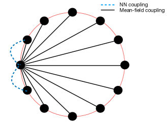
Figure 1: (Color online) Schematic diagram showing the coupling scheme for the model (1) on a one-dimensional periodic lattice. The phase oscillators occupying the lattice sites (black filled circles) have a mean-field and a nearest-neighbor coupling. For a representative site, we have shown by black full lines (respectively, by blue dashed lines) the mean-field (respectively, the nearest-neighbor (NN)) coupling.

We consider a one-dimensional periodic lattice of $L$ sites, with sites labeled $i=1,2\ldots,L$. On each site resides a phase oscillator interacting with oscillators on all other sites via a mean-field coupling with strength $J$ and also with oscillators on its nearest-neighbor sites with strength $K$. Figure 1 shows the coupling scheme. We take $J$ to be positive, while $K$ can be of either sign. Denoting by $\theta_{i}\in[0,2\pi);~{}\theta_{i+L}=\theta_{i}$ the angle not (a) of the oscillator on the $i$-th site, the dynamics is defined by $L$ coupled nonlinear differential equations of the form

$$\frac{{\rm d}\theta_{i}}{{\rm d}t}=\omega_{i}+Jr\sin(\psi-\theta_{i})+K\sum_{j\in nn_{i}}\sin(\theta_{j}-\theta_{i}).$$ (1)

Here, $\omega_{i}$ is the natural frequency of the $i$-th oscillator, while the second term on the right hand side (rhs) may be interpreted as a torque (in suitable units) arising from a mean-field interaction and expressed in terms of the usual Kuramoto synchronization order parameter Kuramoto (1984); Strogatz (2000)

$$re^{{\rm i}\psi}\equiv\frac{1}{L}\sum_{j=1}^{L}e^{{\rm i}\theta_{j}}.$$ (2)

On the other hand, the third term on the rhs of Eq. (1) is the torque due to a nearest-neighbor interaction, with the sum over $j$ restricted to the nearest neighbors of $i$. The $\omega_{i}$’s denote a set of quenched-disordered random variables sampled independently from a common distribution $G(\omega)$ with finite mean $\omega_{0}>0$ and width $\sigma>0$. The quantity $r;~{}0\leq r\leq 1$ in Eq. (2) is a measure of the amount of synchrony present in the system at a given time instant, while $\psi$ measures the average angle Strogatz (2000). As is usual in studies of the Kuramoto model, we consider $G(\omega)$ to be unimodal, i.e., symmetric about $\omega_{0}$ and decreasing monotonically and continuously to zero with increasing $|\omega-\omega_{0}|$. In view of rotational invariance of the dynamics (1), the effect of $\omega_{0}$ can be gotten rid of from the dynamics by effecting the transformation $\theta_{i}\to\theta_{i}+\omega_{0}t~{}\forall~{}i$. On implementing such a transformation, one evidently has $\omega_{i}$’s having zero mean in the resulting dynamics; we will from now on consider such an implementation to have been made, and consider instead of (1) the dynamics

$$\frac{{\rm d}\theta_{i}}{{\rm d}t}=\sigma\omega_{i}+Jr\sin(\psi-\theta_{i})+K\sum_{j\in nn_{i}}\sin(\theta_{j}-\theta_{i}).$$ (3)

Here, the $\omega_{i}$’s are now distributed according to a distribution $g(\omega)$ that has zero mean and unit variance.

The dynamics (3) is intrinsically non-Hamiltonian. This may be understood as follows: although the torque due to the mean-field and the nearest-neighbor interaction may be obtained from a potential $V(\{\theta_{i}\})\equiv(J/2L)\sum_{i,j=1}^{L}[1-\cos(\theta_{i}-\theta_{j})]-K\sum_{i=1}^{L}[\cos(\theta_{i+1}-\theta_{i})+\cos(\theta_{i-1}-\theta_{i})]$, a similar procedure cannot be implemented for the frequency term. This is because an ad hoc potential $\sim-\sum_{i=1}^{L}\sigma\omega_{i}\theta_{i}$ that would nevertheless allow to obtain the frequency term in the dynamics (3) would not be periodic in the angle variables and thus cannot be regarded as a bona fide potential of the system. As a result of the foregoing, the dynamics (3) cannot be interpreted as an overdamped dynamics on a potential landscape, as is possible with $\omega_{i}=0~{}\forall~{}i$ Gupta et al. (2018). In the latter case, the dynamics may be written as

$$\frac{{\rm d}\theta_{i}}{{\rm d}t}=-\frac{\partial V(\{\theta_{i}\})}{\partial\theta_{i}},$$ (4)

and then the long-time stationary solution corresponds to values of $\theta_{i}$’s that minimize the potential $V(\{\theta_{j}\})$ Strogatz (2014). A consequence of the non-Hamiltonian nature of the dynamics (3) is that the stationary state it relaxes to is not an equilibrium but rather a nonequilibrium stationary state Gupta et al. (2018).

Setting $K$ to zero in Eq. (3) recovers the usual Kuramoto model that has only mean-field interaction Kuramoto (1984); Acebrón et al. (2005); Gupta et al. (2014); Rodrigues et al. (2016); Gupta et al. (2018), while setting $J$ to zero reduces the dynamics to the version of the Kuramoto model with only nearest-neighbor interaction Strogatz and Mirollo (1988). In the former case, it is known in the limit $L\to\infty$ that in the stationary state, attained as $t\to\infty$, the model shows a continuous phase transition from a low-$J$ incoherent phase (zero value of the stationary $r$) to a high-$J$ synchronized phase (a non-zero value for the stationary $r$) across the critical point $J_{c}=2\sigma/(\pi g(0))$ Strogatz (2000); Gupta et al. (2018). Study of the model with only nearest-neighbor interaction has established that in the limit $L\to\infty$, no angle locking and consequently, a non-zero value for stationary $r$ is possible Strogatz and Mirollo (1988).

III Reparametrization of the dynamics and queries

For further analysis, we reduce the dynamics (3) to a dimensionless form. To this end, implementing for $J\neq 0$ the transformations $t\to Jt,~{}\sigma\to\sigma/J,~{}K\to K/J$, one obtains the dimensionless form as

$$\frac{{\rm d}\theta_{i}}{{\rm d}t}=\sigma\omega_{i}+r\sin(\psi-\theta_{i})+K\sum_{j\in nn_{i}}\sin(\theta_{j}-\theta_{i}).$$ (5)

The aforementioned transformations are tantamount to considering the dynamics (3) with $J=1$. We will show later in this section that the relevant parameters to obtain phase transitions in the dynamics (3) are the ratios $\sigma/J$ and $K/J$, and hence, the results on the order parameter variation when plotted, e.g., as a function of $K/J$ and for a fixed $\sigma/J$, with different values of $J\neq 0$, all coincide. The latter fact justifies the transformations that have been invoked to rewrite the dynamics in the form (5). From now on, we will study the dynamics (5) in the parameter space $(\sigma,K)$. In obtaining numerical results reported later in the paper, we employ as representative examples of the frequency distribution a Gaussian and a Lorentzian $g(\omega)$; $\sigma$ is identified with the variance of the Gaussian distribution, and with the half-width at half-maximum of the Lorentzian distribution.

In the dimensionless dynamics (5), the continuous transition of the usual Kuramoto model is observed as one tunes $\sigma$ across the critical value $\sigma_{c}=\pi g(0)/2$, with the system existing in the synchronized phase at low $\sigma$ and in the incoherent phase at high $\sigma$. In this backdrop, we ask: How does the inclusion of nearest-neighbor interaction modify the stationary-state phase diagram? Do new phases emerge? What is the order of transition between the different phases? We may anticipate new features in view of the fact that for $K<0$, the mean-field and nearest-neighbor interactions have competing tendencies: while the former favors global synchrony, the latter would like to make oscillator angles get out of phase on nearest-neighbor sites. For $K>0$, however, we expect both the mean-field and the local interaction to have cooperative effect in establishing global synchrony. In both the scenarios, an essential role will be played also by the parameter $\sigma$. In view of the foregoing, it is evidently pertinent to embark on a detailed analysis of the dynamics (5), an issue we take up in this work. The results presented in the whole of Section IV correspond to Gaussian $g(\omega)$, while the case of Lorentzian $g(\omega)$ is discussed in Section VI.

IV Phase diagram of the model (5) in ($\sigma-K$) plane

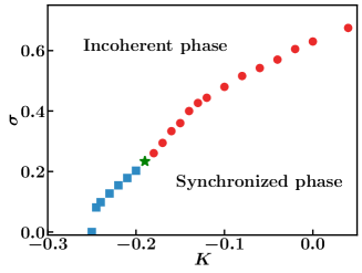
Figure 2: (Color online) The complete phase diagram of the model (5) in the ($\sigma-K$) plane, showing synchronized and incoherent phases separated by a line of transition that is either first-order (blue squares) or continuous (red circles). The two lines meet at a tricritical point, shown by a green star. The frequency distribution $g(\omega)$ is a Gaussian with zero mean and unit variance. Exact results are obtained for (i) $K=0$, yielding the critical point $(\sigma_{c}=\sqrt{\pi}/(2\sqrt{2}),0)$, and (ii) $\sigma=0$, yielding the critical point $(K_{c}=-0.25,\sigma=0)$.

The stationary-state phase diagram of the model (5) in the ($\sigma-K$) plane is shown in Fig. 2 for Gaussian $g(\omega)$, where the circles in red constitute the line of continuous transition, while the line of first-order transition is represented by squares in blue. The tricritical point is located at ($\sigma_{\rm Tricritical}\approx 0.23,~{}K_{\rm Tricritical}\approx-0.19$), and is denoted by a green star. We discuss below how we obtain the phase diagram in Fig.  2 from numerical integration results of the dynamics (5) for large but finite $L$. For the system sizes scanned, we did not observe any appreciable dependence of the transition points on $L$.

From the phase diagram, we see that for $K>0$, when both the mean-field and the nearest-neighbor interaction favour global synchrony, one has a continuous phase transition from a low-$\sigma$ synchronized phase to a high-$\sigma$ incoherent phase. For negative values of $K$, there is instead a competition between the two types of interaction. One has a continuous transition as long as $K>K_{\rm Tricritical}$ and otherwise a first-order transition. As stated earlier, for $K=0$, we recover the transition point of the usual Kuramoto model.

For $\sigma=0$, we now discuss how one may obtain exact results for the critical value $K_{c}$. In this case, the dynamics (5) takes the form of Eq. (4), with the potential in dimensionless form given by

$$V(\{\theta_{i}\})=-r\sum_{i=1}^{L}\cos(\psi-\theta_{i})$$

$$-K\sum_{i=1}^{L}[\cos(\theta_{i+1}-\theta_{i})+\cos(\theta_{i-1}-\theta_{i})].$$ (6)

As mentioned in Section II, the stationary solution then corresponds to values of $\theta_{i}$’s that minimize the potential $V$. Consider first the incoherent phase, which has by definition a zero value for stationary $r$, and the potential is minimized by having angles of oscillators on nearest-neighbor sites differing by an amount equal to $\pi$ (since $K$ is here negative, see Fig. 2). The corresponding minimum value of the potential (6) is given by

$$V_{\rm inc}=2KL.$$ (7)

On the other hand, the potential can also be minimized by having all the angles equal to one another (which is the favored state for $\sigma=0$), yielding unity for the stationary $r$ (maximally synchronized phase) and the potential having the corresponding value

$$V_{\rm sync}=-L-2KL.$$ (8)

It is then evident that equating $V_{\rm inc}$ with $V_{\rm sync}$ defines $K_{c}$ such that on either side of this critical value, it is the incoherent or the synchronized phase that minimizes the potential and is consequently observed in the stationary state. The equality $2K_{c}L=-L-2K_{c}L$ yields the exact critical value $K_{c}=-0.25$.

The rest of this section is devoted to a detailed discussion of how one may obtain the phase diagram in Fig. 2 from an analysis of the dynamics (5).

IV.1 Continuous versus first-order transitions

In order to gain preliminary insights into possible dynamical behavior, one may start off with performing numerical integration of the dynamics (5) by employing a fourth-order Runge-Kutta algorithm with integration time step ${\rm d}t=0.01$ and for Gaussian $g(\omega)$. Figure 3(a) shows for several values of $\sigma$ the variation of the order parameter $r$ with $K$ in the stationary state on a lattice of size $L=3200$ not (b). In obtaining the results depicted in the figure, we initiate, for every individual pair of values of $\sigma$ and $K$, the dynamics (5) in a state in which all the oscillators have the same angle; we then let the system relax to stationarity, signalled by a time-independent value of $r$, and record the latter value. Unless stated otherwise, the results for the order parameter presented here and elsewhere in the paper have been obtained by taking time average of the data in the stationary state for a given frequency realization $\{\omega_{i}\}$ and considering a further average over different frequency realizations. The figure suggests the existence of both synchronized and incoherent phases and a phase transition between them. The latter appears to be continuous (continuous variation) for high values of $\sigma$, and to be first-order-like (sharp jump) for low $\sigma$.

Our phase diagram 2 clearly shows that varying $K$ at a fixed $\sigma$ lets us reveal the nature of the phase transition in a way that is completely equivalent to varying $\sigma$ at a fixed $K$. That this is indeed the case is evident from the results presented in Fig. 3(b) that shows for several values of $K$ the variation of the order parameter $r$ with $\sigma$ in the stationary state on a lattice of size $L=3200$ not (b). Again, we see both synchronized and incoherent phases, with a phase transition between them that appears to be continuous for positive and low negative values of $K$, and to be first-order-like for large negative $K$.

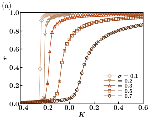
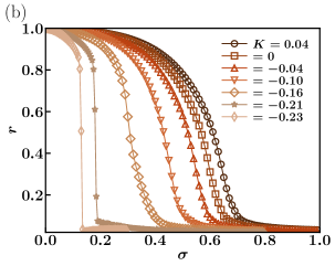
Figure 3: (Color online) Variation of order parameter $r$ with $K$ for several values of $\sigma$ (panel (a)) and that with $\sigma$ for several values of $K$ (panel (b)) in the stationary state of the dynamics (5) on a lattice of size $L=3200$. The frequency distribution $g(\omega)$ is a Gaussian with zero mean and unit variance. The data have been averaged, first over dynamical evolution in the stationary state for a given frequency realization $\{\omega_{i}\}$, and then over different frequency realizations. Both the figures suggest the existence of both synchronized and incoherent phases and a phase transition between them. The latter appears to be continuous (continuous variation of $r$) for high values of $\sigma$, and to be first-order-like (sharp jump of $r$) for low $\sigma$, as shown in panel (a). Similarly, the figure in panel (b) shows that the transition from the synchronized to the incoherent phase appears continuous for positive and low negative values of $K$ and first-order-like for large negative $K$. The data are obtained from numerical integration of the dynamics (5). In obtaining the results depicted in the figure, we initiate, for every individual pair of values of $\sigma$ and $K$, the dynamics (5) in a state in which all the oscillators have the same angle; we then let the system relax to stationarity, signalled by a time-independent value of $r$, and record the latter value.

Since a clear distinguishing feature between first-order and continuous transitions is the occurrence of hysteresis in the former Binder (1987), we now proceed to report on results of such a study. Numerical results reported in Fig. 4 correspond to the situation in which for a fixed value of $\sigma$, we let the system relax to the stationary state at $\sigma=0$ while starting from an initial state in which all the oscillators have the same angle, and then tune $\sigma$ adiabatically to high values and back in a cycle, while recording concomitantly the value of the order parameter $r$. Adiabatic tuning ensures that the system is at every instant of time close to a stationary state as $\sigma$ is tuned in time. Figures 4(a),(b) show the variation of $r$ with adiabatically-tuned $\sigma$, for $K=0.04$ and $K=-0.1$, respectively. In both cases, the curves corresponding to forward and backward variation of $\sigma$ coincide up to numerical precision, and consequently, we do not observe any hysteresis behavior, thereby hinting at the corresponding transition from the synchronized to the incoherent phase being a continuous one. On the other hand, results displayed in Figs. 4(c),(d) for $K=-0.21$ and $-0.23$, respectively, show the existence of a hysteresis loop, thereby bearing a clear signature of a first-order transition. It may be noted from the results for the backward variation of $\sigma$ shown in panels (c) and (d) that $r$ does not attain the value of unity as $\sigma$ is reduced to zero, but instead has a value close to zero. We understand this as due to the system being stuck in long-lived metastable states during relaxation to a synchronized state for $K$ negative and large in magnitude. To illustrate this point, consider the plots in Fig. 5 for a large negative value of $K$ and at a fixed $\sigma$ at which an initial synchronized state is stable. The figure shows time evolution of $r$ for several realizations of an initial incoherent state. It may be seen that only a fraction $\eta$ of these realizations relax to the synchronized state over the time window of observation, with the fraction decreasing fast with the increase of system size $L$ (inset of Fig. 5). This result implies that in the limit of large $L$, the system does not exhibit relaxation to the synchronized state but remains close to the initial incoherent state, consistent with the results displayed in Fig. 4, panels (c) and (d).

Figure 6 shows the variation of the order parameter $r$ with adiabatically-tuned $K$ in the stationary state of the dynamics (5) for two values of $\sigma$, namely, $\sigma=0.1$ (panel (a)), and $\sigma=0.5$ (panel (b)). Hysteresis behaviour is observed only in panel (a) and not in panel (b), consistent with the fact that for $\sigma=0.1$ (respectively, $\sigma=0.5$), one has a first-order (respectively, a continuous) transition, see Fig. 2. As claimed following Eq. (5), Fig. 7 demonstrates that the relevant parameters to obtain our observed phase transitions for the model (3) are the ratios $\sigma/J$ and $K/J$, as a result of which $r$ when plotted as a function of $K/J$ and for a fixed $\sigma/J$, with different values of $J\neq 0$, all coincide. This justifies the transformations invoked in reducing the dynamics (3) to (5).

One may wonder as to why the plots in Fig. 3 corresponding to first-order transitions do not show hysteresis, while the ones in Figs. 4 and 6 do show hysteresis. To understand this, attention may be called to the fact the plots in Fig. 3 do not correspond to adiabatic tuning of the parameter plotted in the $x$-axis. For example, the plots of $r$ versus $K$ at a given value of $\sigma$ correspond of several independent numerical runs at the given $\sigma$ for each of which $K$ is fixed at given values, letting each run relaxing the system to stationarity and recording the corresponding stationary value of $r$. In contrast, the plots in, e.g., Fig. 6 correspond to a single numerical run in which in the stationary state and for a fixed $\sigma$, the parameter $K$ is continuously and adiabatically tuned in time and the corresponding value of $r$ is recorded. As follows from the theory of first-order phase transitions Binder (1987), it is only in the latter case of adiabatic tuning that one should observe hysteresis and not in the case of Fig. 3.

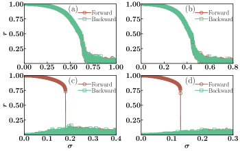
Figure 4: (Color online) Variation of order parameter $r$ with adiabatically-tuned $\sigma$ in the stationary state of the dynamics (5) on a lattice of size $L=3200$ and for four values of $K$, namely, $K=0.04$ (panel (a)), $K=-0.1$ (panel (b)), $K=-0.21$ (panel (c)), and $K=-0.23$ (panel (d)). The frequency distribution $g(\omega)$ is a Gaussian with zero mean and unit variance. The results correspond to a typical realization of the frequencies. Hysteresis behaviour is observed only in panels (c) and (d). The data are obtained from numerical integration of the dynamics (5).

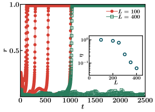
Figure 5: (Color online) Considering the dynamics (5) for a large negative value of $K$ (namely, $K=-0.21$) and at a fixed $\sigma$ at which an initial synchronized state is stable (we have taken $\sigma=0.05$), the main figure shows for two system sizes the time evolution of $r$ for five realizations of an initial incoherent state. The frequency distribution $g(\omega)$ is a Gaussian with zero mean and unit variance. It may be seen that with increase of $L$, a smaller number of initial realizations relax to the synchronized state over the time window of observation. The inset shows this fraction $\eta$ as a function of $L$, indicating fast decrease with increase of $L$. This result implies that in the limit of large $L$, the system does not exhibit relaxation to the synchronized state but remains close to the initial incoherent state, consistent with the results displayed in Fig. 4, panels (c) and (d). The data are obtained from numerical integration of the dynamics (5).

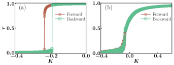
Figure 6: (Color online) Variation of order parameter $r$ with adiabatically-tuned $K$ in the stationary state of the dynamics (5) on a lattice of size $L=3200$ and for two values of $\sigma$, namely, $\sigma=0.1$ (panel (a)), and $\sigma=0.5$ (panel (b)). The frequency distribution $g(\omega)$ is a Gaussian with zero mean and unit variance. The results correspond to a typical realization of the frequencies. Hysteresis behaviour is observed only in panel (a) and not in panel (b), consistent with the fact that for $\sigma=0.1$ (respectively, $\sigma=0.5$), one has a first-order (respectively, a continuous) transition, see Fig. 2. The data are obtained from numerical integration of the dynamics (5).

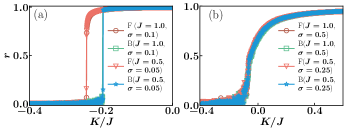
Figure 7: (Color online) Variation of order parameter $r$ with adiabatically-tuned $K$, rescaled by $J$, in the stationary state of the dynamics (3) on a lattice of size $L=3200$. The values of $J$ and $\sigma$ are mentioned in the individual panels for both forward (F) and backward (B) variation of $K$ in time. The frequency distribution $g(\omega)$ is a Gaussian with zero mean and unit variance. The results correspond to a typical realization of the frequencies. The data are obtained from numerical integration of the dynamics (3). The results are a clear demonstration of the fact that the relevant parameters to obtain phase transitions for the model (3) are the ratios $\sigma/J$ and $K/J$, as a result of which $r$ when plotted as a function of $K/J$ and for a fixed $\sigma/J$, with different values of $J\neq 0$, all coincide. This justifies the transformations invoked in reducing the dynamics (3) to (5).

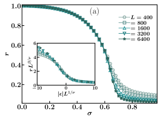
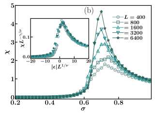
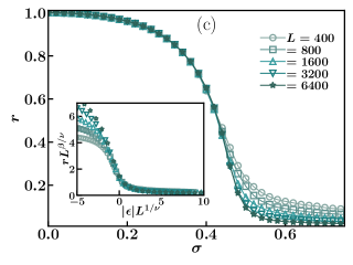
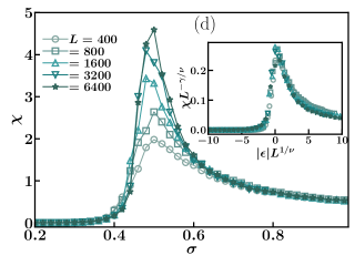
Figure 8: (Color online) For two values of $K$, the figure shows the variation with $\sigma$ of the finite-$L$ order parameter $r\equiv r(L)$ and the quantity $\chi\equiv\chi(L)$ (see Eq. (9)) in the stationary state of the model (5), for five values of the system size $L$. In the insets, we show scaling collapse of the data according to Eq. (10). The frequency distribution $g(\omega)$ is a Gaussian with zero mean and unit variance. We have $K=0.04$ for panels (a) and (b) and $K=-0.1$ for panels (c) and (d). The data involve time averaging in the stationary state for a given frequency realization $\{\omega_{i}\}$ as well as over different frequency realizations. The critical point $\sigma_{c}\equiv\sigma_{c}(K)$ is obtained by plotting the maximum of $\chi(L)$ as a function of $L$ and fitting it to a power law, while the values of the critical exponents $\beta,\nu,\gamma$ are obtained from the scaling collapse of the data for $r$ and $\chi$. The data are obtained from numerical integration of the dynamics (5).

On the basis of the foregoing, we may conclude the existence of both continuous and first-order phase transitions in the stationary state of the dynamics (5). Our next task would be to explain how we obtain numerically the phase-transition lines in the $(\sigma,K)$-plane, as shown in Fig. 2, and to explain in particular how we locate the tricritical point, defined as the point at which the first-order and continuous transition lines meet. In the following, we will discuss the phase diagram and the phase transitions presented therein by varying $\sigma$ at a fixed $K$, though we emphasize that this way of uncovering the nature of the phase transition is completely equivalent to varying $K$ at a fixed $\sigma$, with the latter being perhaps more amenable to experimental implementation; the equivalence is evidently true from the phase diagram 2.

IV.2 Obtaining the line of continuous transition

In order to locate numerically the line of continuous transition, we proceed as follows. At values of $K$ at which no hysteresis is observed in the variation of $r$ with adiabatically-tuned $\sigma$, our aim is to estimate the value of $\sigma_{c}\equiv\sigma_{c}(K)$, namely, the value of $\sigma$ at the critical point of transition at fixed $K$. To this end, we analyze the finite-$L$ data for stationary $r$ by resorting to the finite-size scaling theory for equilibrium critical phenomena briefly summarized in Appendix B. By drawing an analogy with Eq. (41), we write scaling forms for the order parameter $r(L)$ obtained in a system of size $L$ and the stationary-state temporal fluctuations of the order parameter defined as

$$\chi(L)\equiv L~{}\overline{\langle r^{2}(L)\rangle-\langle r(L)\rangle^{2}},$$ (9)

where the angular brackets and the overbar denote respectively time average in the stationary state for a given frequency realization $\{\omega_{i}\}$ and average over frequency realizations. The scaling forms are

$$r(L)\sim L^{-\beta/\nu}f(|\epsilon|L^{1/\nu}),$$

(10)

$$\chi(L)\sim L^{\gamma/\nu}g(|\epsilon|L^{1/\nu}),$$

with $\beta,\nu,\gamma$ being the critical exponents, and

$$\epsilon\equiv\frac{\sigma-\sigma_{c}}{\sigma_{c}}.$$ (11)

As discussed in Appendix B, the scaling functions $f(x)$ and $g(x)$, defined with $x>0$, behave in the limit $x\to\infty$ as $f(x)\sim x^{\beta}$ and $g(x)\sim x^{-\gamma}$. In the limit $x\to 0$, both the functions behave as constants.

Now, following the procedure detailed in Appendix B to obtain the critical point, $\sigma_{c}\equiv\sigma_{c}(K)$ is estimated from the plot of the maximum of $\chi(L)$ as a function of $L$ and fitting it to a power law. Using the value of $\sigma_{c}$ estimated this way, and requiring for large $L$ scaling collapse of the finite-$L$ data for $r(L)$ and $\chi(L)$ according to the forms in Eq. (10) allow to obtain values for the critical exponents $\beta,\gamma,\nu$. In Fig. 8, we show for two values of $K$ the behavior of $r$ (panels (a) and (c)) and $\chi$ (panels (b) and (d)) as a function of $\sigma$ and scaling collapse in the corresponding insets. We have $K=0.04$ for panels (a) and (b) and $K=-0.1$ for panels (c) and (d). The values of the critical exponents that yielded scaling collapse are: for $K=0.04$, we have $\beta\approx 0.52,\nu\approx 2.0,\gamma\approx 0.76$, while for $K=-0.1$, we have $\beta\approx 0.78,\nu\approx 3.13,\gamma\approx 1.06$. We note that one requires data for larger $L$ in order to estimate more reliably the critical exponent values. Our focus here is primarily on establishing the existence of a continuous phase transition in the dynamics (5) for a range of values of $K$, and in this regard, a confirmation, in addition to the no-hysteresis data presented in Fig. 4, is provided by the very good scaling collapse for large $L$ demonstrated in Fig. 8 for which the underlying theory invoked is that of finite-size scaling for continuous transitions. That we have been able to estimate $\sigma_{c}$ accurately is evident from the quality of scaling collapse seen in Fig. 8.

The aforementioned procedure of obtaining $\sigma_{c}(K)$ from the data of $\chi(L)$ is repeated for several values of $K$ at which one does not observe any hysteresis in the behavior of $r$ as a function of adiabatically-tuned $\sigma$. In this way, we obtain the values of $\sigma_{c}(K)$ as a function of $K$, which we use to construct the phase diagram in the $(\sigma,K)$-plane, that is, draw the line of continuous transition, see Fig. 2.

IV.3 Obtaining the line of first-order transition

Having obtained in the preceding section the line of continuous transition, we now proceed to obtain the line of first-order transition. In the absence of a scaling theory akin to the one that exists on general grounds for continuous transitions, we proceed to obtain the first-order transition point as follows. At a first-order phase transition, the order parameter as a function of time shows bistability, with the system switching back and forth between two phases. For our system (5), we show in Fig. 9(a) the behavior of $r$ versus time in the stationary state and at a value of $K$ at which we have observed hysteresis (cf. Fig. 4). Such a bistable behavior may be characterized by drawing the probability distribution $P(r)$ of stationary $r$. When bistable, $P(r)$ is bimodal with two peaks of equal heights. Contrarily, while on either side of the transition point when the system is no more bistable, the distribution $P(r)$ is bimodal, but the peaks are not of equal heights. Considering our model (5), when one is at a value of $\sigma$ smaller (respectively, greater) than the critical value of first-order transition, $P(r)$ will have a higher peak at a value of $r$ corresponding to the synchronized (respectively, incoherent) phase. Then, in order to locate the transition point, we adopt the following strategy. For a fixed $K$ and a given (large) system size $L$, we scan the range of $\sigma$, obtaining for each value the distribution $P(r)$ from the time variation of $r$ in the stationary state, and estimate the transition point as the value of $\sigma$ at which $P(r)$ has two peaks of equal heights. An example is shown in Fig. 9(b). Note that unlike a first-order transition point that is characterized by two equally likely values of the order parameter, a continuous transition is characterized by a distribution $P(r)$ that is single peaked, with the peak shifting continuously from non-zero to zero values as $\sigma$ is tuned from below to above the transition point.

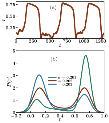
Figure 9: (Color online) Time variation of the order parameter $r$ (panel (a)) and the corresponding distribution $P(r)$ (panel (b)) in the stationary state of the dynamics (5) and at a value of $K$ (namely, $K=-0.202$) at which one has a first-order transition. The system size is $L=3200$. The frequency distribution $g(\omega)$ is a Gaussian with zero mean and unit variance. The results correspond to a typical realization of the frequencies. Exactly at the transition point, the distribution has two peaks of equal height, while on either side, the peaks have different heights. Note that the switching time between the two bistable states, as in panel (a), becomes with increasing $L$ so prohibitively large that one does not observe enough switching within a reasonable time interval of observation, and then, one does not have enough statistics to draw the distribution $P(r)$. The data are obtained from numerical integration of the dynamics (5).

The above background on how to locate first-order and continuous transition points in the $(\sigma,K)$-plane armed us to draw in Fig. 2 the corresponding transition lines and to locate the tricritical point at which the two lines meet.

In the following section, we embark on an analysis of the dynamics (5) based on an approximate theory that allows to obtain the behavioral trend of the order parameter in the stationary state.

V Theoretical analysis

In this section, we discuss a suitably-modified version of an approximate time-averaged theory proposed in Restrepo et al. (2005), see also Rodrigues et al. (2016), which allows to obtain quite accurately the behavior of the order parameter in the stationary state of our model (5) in parameter regimes of continuous transitions. To proceed, let us define a weighted adjacency matrix as

$$W_{ij}\equiv\frac{1}{L}(1-\delta_{ij})+K\delta_{i,j\pm 1};~{}~{}i,j=1,2,\ldots,L,$$ (12)

in terms of which we rewrite Eq. (5) as

$$\frac{{\rm d}\theta_{i}}{{\rm d}t}=\sigma\omega_{i}+{\rm Im}\left[e^{-i\theta_{i}}\sum_{j=1}^{L}W_{ij}e^{i\theta_{j}}\right].$$ (13)

Let us now consider the above dynamics in the stationary state, and express it as

$$\frac{{\rm d}\theta_{i}}{{\rm d}t} = \sigma\omega_{i}+r_{i}^{({\cal T})}\sin(\psi_{i}-\theta_{i})+h_{i}(t),$$ (14)

where we have defined a time-averaged local order parameter for the $i$-th site as

$$r_{i}^{({\cal T})}e^{i\psi_{i}}\equiv\sum_{j=1}^{L}W_{ij}\langle e^{i\theta_{j}}\rangle$$

$$=re^{i\psi}+K\left(\langle e^{i\theta_{i+1}}\rangle+\langle e^{i\theta_{i-1}}\rangle\right)-\frac{1}{L}\langle e^{i\theta_{i}}\rangle,$$ (15)

with the angular brackets denoting as usual time average over dynamics in the stationary state for a given frequency realization $\{\omega_{i}\}$, while $h_{i}(t)$ denotes stationary-state fluctuations:

$$h_{i}(t)\equiv{\rm Im}\left[e^{-i\theta_{i}}\sum_{j=1}^{L}W_{ij}\left(e^{i\theta_{j}}-\langle e^{i\theta_{j}}\rangle\right)\right].$$ (16)

In obtaining the first term on the rhs of Eq. (15), we have used the fact that since we are in the stationary state, we have $\langle re^{i\psi}\rangle=re^{i\psi}$. Note that the quantities $r_{i}^{({\cal T})}$ and $\psi_{i}$ are by definition time independent.

The time-averaged theory aims to study the synchronized phase by neglecting for large $L$ the fluctuations $h_{i}(t)$ in the dynamics (14) Restrepo et al. (2005); Rodrigues et al. (2016), which therefore reads

$$\frac{{\rm d}\theta_{i}}{{\rm d}t}=\sigma\omega_{i}+r_{i}^{({\cal T})}\sin(\psi_{i}-\theta_{i}).$$ (17)

Considering the dynamics (17), it is well known from the study of a similar equation occurring in the usual Kuramoto model Strogatz (2000); Gupta et al. (2018) that if the $i$-th oscillator has $r_{i}^{({\cal T})}$ having such a value that $\sigma|\omega_{i}|\leq r_{i}^{({\cal T})}$, the quantity $\theta_{i}-\psi_{i}$ would have a stable fixed point given by $\sin(\theta_{i}-\psi_{i})=\sigma\omega_{i}/r_{i}^{({\cal T})};~{}\cos(\theta_{i}-\psi_{i})=+\sqrt{1-\sigma^{2}\omega_{i}^{2}/(r_{i}^{({\cal T})})^{2}}$, the latter determining the value of $\theta_{i}-\psi_{i}$ in the stationary state. All such oscillators satisfying $\sigma|\omega_{i}|\leq r_{i}^{({\cal T})}$ are therefore called phase-locked or synchronized oscillators. On the other hand, oscillators with $\sigma|\omega_{i}|>r_{i}^{({\cal T})}$ constitute the so-called drifting oscillators, for which the dynamics (17) does not allow for a stable fixed point.

Let $\rho_{j}(\theta)d\theta$ denote the stationary probability that the $j$-th oscillator, with its natural frequency equal to $\omega_{j}$, has its angle in the range ($\theta,\theta+{\rm d}\theta$). If the $j$-th oscillator is phase locked, the normalized density is given by Acebrón et al. (2005); Gupta et al. (2018)

$$\rho_{j}^{\rm locked}(\theta-\psi) = r_{j}^{({\cal T})}\cos(\theta-\psi)\delta\left(\sigma\omega_{j}-r_{j}^{({\cal T})}\sin(\theta-\psi)\right)$$ (18)

$$\times\Theta\left(\cos(\theta-\psi)\right),$$

with $\Theta(x)$ being the Heaviside step function. On the other hand, the probability density in the case that the $j$-th oscillator is drifting is given by Acebrón et al. (2005); Gupta et al. (2018)

$$\rho_{j}^{\rm drift}(\theta-\psi)=\frac{1}{2\pi}\frac{\sqrt{\sigma^{2}{\omega_{j}}^{2}-(r_{j}^{({\cal T})})^{2}}}{|\sigma\omega_{j}-r_{j}^{({\cal T})}\sin(\theta-\psi)|}.$$ (19)

The value of $r_{i}^{({\cal T})}$ may then be found self-consistently as

$$r_{i}^{({\cal T})}=r_{i}^{(\cal T)}\big{|}_{\rm locked}+r_{i}^{(\cal T)}\big{|}_{\rm drift}$$

$$=\sum_{j;~{}\sigma|\omega_{j}|\leq r_{j}^{({\cal T})}}W_{ij}\langle e^{i(\theta_{j}-\psi_{i})}\rangle+\sum_{j;~{}\sigma|\omega_{j}|>r_{j}^{({\cal T})}}W_{ij}\langle e^{i(\theta_{j}-\psi_{i})}\rangle.$$

(20)

The contribution of the locked oscillators to the order parameter is calculated as follows:

$$r_{i}^{({\cal T})}\big{|}_{\rm locked}=\sum_{j;~{}\sigma|\omega_{j}|\leq r_{j}^{({\cal T})}}W_{ij}\langle e^{i(\theta_{j}-\psi_{j})}e^{i(\psi_{j}-\psi_{i})}\rangle.$$ (21)

These oscillators have $\theta_{j}-\psi_{j}$ taking up time-independent values in the stationary state, so that the corresponding factor may be taken out of the angular brackets in Eq. (21), Moreover, $\psi_{i}$ and $\psi_{j}$ being time independent, we have $\langle e^{i(\psi_{j}-\psi_{i})}\rangle=e^{i(\psi_{j}-\psi_{i})}$. The time-independent values for $\theta_{j}-\psi_{j}$ are distributed according to the delta-function distribution (18), implying that we have $(\theta_{j}-\psi_{j})=\sin^{-1}\left(\sigma\omega_{j}/r_{j}^{({\cal T})}\right);~{}\cos(\theta_{j}-\psi_{j})=+\sqrt{1-\sigma^{2}\omega_{j}^{2}/(r_{j}^{({\cal T})})^{2}}$). Putting all these together, we have

$$r_{i}^{({\cal T})}\big{|}_{\rm locked} = \sum\limits_{j;~{}\sigma|\omega_{j}|\leq r_{j}^{({\cal T})}}W_{ij}e^{i(\psi_{j}-\psi_{i})}$$ (22)

$$\times\left[\left(\sqrt{1-\frac{\sigma^{2}\omega_{j}^{2}}{(r_{j}^{({\cal T})})^{2}}}\right)+i\left(\frac{\sigma\omega_{j}}{r_{j}^{({\cal T})}}\right)\right].$$

Proceeding in the same manner as for the locked oscillators, we may obtain the contribution of the drifting oscillators:

$$r_{i}^{({\cal T})}\big{|}_{\rm drift}=\sum_{j;~{}\sigma|\omega_{j}|>r_{j}^{({\cal T})}}W_{ij}\langle e^{i(\theta_{j}-\psi_{j})}e^{i(\psi_{j}-\psi_{i})}\rangle$$

$$=\sum_{j;~{}\sigma|\omega_{j}|>r_{j}^{({\cal T})}}W_{ij}e^{i(\psi_{j}-\psi_{i})}\langle e^{i(\theta_{j}-\psi_{j})}\rangle$$

$$=\sum_{j;~{}\sigma|\omega_{j}|>r_{j}^{({\cal T})}}W_{ij}e^{i(\psi_{j}-\psi_{i})}\left[\langle\cos(\theta_{j}-\psi_{j})\rangle+i\langle\sin(\theta_{j}-\psi_{j})\rangle\right].$$

(23)

Now, the drifting oscillators, unlike the locked ones, do not have time-independent values for their angle $\theta_{j}-\psi_{j}$, but instead have their values distributed according to the stationary distribution (19). Consequently, in computing the time average $\langle e^{i(\theta_{j}-\psi_{j})}\rangle$, we need to consider that $(\theta_{j}-\psi_{j})$ would take values following the distribution (19), so that we have

$$\langle\cos(\theta_{j}-\psi_{j})\rangle=\int_{0}^{2\pi}{\rm d}(\theta-\psi)~{}\rho_{j}^{\rm drift}(\theta-\psi)\cos(\theta-\psi)=0,$$

(24)

and

$$\langle\sin(\theta_{j}-\psi_{j})\rangle = \int_{0}^{2\pi}{\rm d}(\theta-\psi)\rho_{j}^{\rm drift}(\theta-\psi)\sin(\theta-\psi)$$ (25)

$$= \frac{\sigma\omega_{j}}{r_{j}^{({\cal T})}}\left[1-\sqrt{1-\frac{(r_{j}^{({\cal T})})^{2}}{\sigma^{2}{\omega_{j}}^{2}}}\right],$$

finally yielding

$$r_{i}^{({\cal T})}\big{|}_{\rm drift} =\sum_{j;~{}\sigma|\omega_{j}|>r_{j}^{({\cal T})}}W_{ij}e^{i(\psi_{j}-\psi_{i})}$$ (26)

$$\times\left[i\frac{\sigma\omega_{j}}{r_{j}^{({\cal T})}}\left(1-\sqrt{1-\frac{(r_{j}^{({\cal T})})^{2}}{\sigma^{2}{\omega_{j}}^{2}}}\right)\right].$$

Using Eqs. (22) and (26) in Eq. (20), and then equating real and imaginary parts from both sides of it, we get

$$r_{i}^{({\cal T})}=$$

$$\sum_{j;~{}\sigma|\omega_{j}|\leq r_{j}^{({\cal T})}}W_{ij}\left[\cos(\psi_{j}-\psi_{i})\left(\sqrt{1-\frac{\sigma^{2}\omega_{j}^{2}}{(r_{j}^{({\cal T})})^{2}}}\right)-\sin(\psi_{j}-\psi_{i})\left(\frac{\sigma\omega_{j}}{r_{j}^{({\cal T})}}\right)\right]-\sum_{j;~{}\sigma|\omega_{j}|>r_{j}^{({\cal T})}}W_{ij}\left[\sin(\psi_{j}-\psi_{i})\frac{\sigma\omega_{j}}{r_{j}^{({\cal T})}}\left(1-\sqrt{1-\frac{(r_{j}^{({\cal T})})^{2}}{\sigma^{2}{\omega_{j}}^{2}}}\right)\right],$$

(27)

$$0=$$

$$\sum_{j;~{}\sigma|\omega_{j}|\leq r_{j}^{({\cal T})}}W_{ij}\left[\sin(\psi_{j}-\psi_{i})\left(\sqrt{1-\frac{\sigma^{2}\omega_{j}^{2}}{(r_{j}^{({\cal T})})^{2}}}\right)+\cos(\psi_{j}-\psi_{i})\left(\frac{\sigma\omega_{j}}{r_{j}^{({\cal T})}}\right)\right]+\sum_{j;~{}\sigma|\omega_{j}|>r_{j}^{({\cal T})}}W_{ij}\left[\cos(\psi_{j}-\psi_{i})\frac{\sigma\omega_{j}}{r_{j}^{({\cal T})}}\left(1-\sqrt{1-\frac{(r_{j}^{({\cal T})})^{2}}{\sigma^{2}{\omega_{j}}^{2}}}\right)\right].$$

(28)

The above equations are solved with the choice $\psi_{i}=\psi_{j}~{}\forall~{}i,j$. Equation (28) then reduces to

$$0=\sum_{j}W_{ij}\left(\frac{\sigma\omega_{j}}{r_{j}^{({\cal T})}}\right)-\sum_{j;~{}\sigma|\omega_{j}|>r_{j}^{({\cal T})}}W_{ij}\frac{\sigma\omega_{j}}{r_{j}^{({\cal T})}}\left(\sqrt{1-\frac{(r_{j}^{({\cal T})})^{2}}{\sigma^{2}{\omega_{j}}^{2}}}\right),$$ (29)

while Eq. (27) now reads

$$r_{i}^{({\cal T})}=\sum_{j;~{}\sigma|\omega_{j}|\leq r_{j}^{({\cal T})}}W_{ij}\left(\sqrt{1-\frac{\sigma^{2}\omega_{j}^{2}}{(r_{j}^{({\cal T})})^{2}}}\right).$$ (30)

Equations (29) and (30) are simultaneously satisfied by taking all $r_{i}^{({\cal T})}$’s to be even in $\{\omega_{j}\}$:  $r_{i}^{({\cal T})}(\{\omega_{j}\})=r_{i}^{({\cal T})}(\{-\omega_{j}\})~{}\forall~{}i$ and satisfying Eq. (30). With our choice of $\omega_{j}$’s being sampled from a symmetric $g(\omega):~{}g(\omega)=g(-\omega)$, Eq. (29) is then automatically satisfied for large $L$, as the contributions in the two sums for every pair of positive and negative $\omega_{j}$ cancel each other. The set of $L$ coupled equations (30) when solved numerically determines the set $\{r_{i}^{({\cal T})}\}$. Equation (15) then allows to obtain the order parameter $r$ for a given frequency realization $\{\omega_{j}\}$ as

$$r=\frac{1}{(1+2K)L-1}\left|\sum_{i=1}^{L}r_{i}^{({\cal T})}e^{i\psi_{i}}\right|=\frac{1}{(1+2K)L-1}\left|\sum_{i=1}^{L}r_{i}^{({\cal T})}\right|,$$ (31)

where in the last step we have used the fact that all the $\psi_{i}$’s are equal. Finally, we average the value of $r$ so obtained over different frequency realizations.

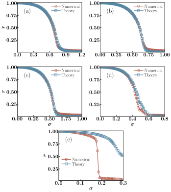
Figure 10: (Color online) The figure shows the variation with $\sigma$ of the stationary order parameter $r$ obtained for the dynamics (5) on a lattice of size $L=3200$, for five values of $K$: $K=0.1$ (panel (a)), $K=0.04$ (panel (b)), $K=-0.04$ (panel (c)), $K=-0.1$ (panel (d)), and $K=-0.21$ (panel (e)). The frequency distribution is a Gaussian with zero mean and unit variance. The figure shows data obtained from numerical integration of the dynamics and from the time-averaged theory discussed in Section V.

We use Eq. (31) to obtain the behaviour of the order parameter $r$ versus $\sigma$ for various values of $K$ and compare with that obtained from direct numerical integration of the dynamics (5) for a lattice of size $L=3200$, see Fig. 10. The values of $K$ are: $K=0.1$ (panel (a)), $K=0.04$ (panel (b)), $K=-0.04$ (panel (c)), $K=-0.1$ (panel (d)), and $K=-0.21$ (panel (e)). The data have been averaged over several frequency realizations. Note that the time-averaged theory described above is valid in the synchronized phase. For positive as well as low negative $K$, the order parameter behaviour obtained from the theory is in very good agreement with numerics, see Fig. 10, panels (a), (b) and (c). With $K$ becoming more negative so that one approaches the tricritical point (see Fig. 2), the deviation between theory and numerics becomes evident, especially close to the phase transition point, see Fig. 10(d). For $K$ values for which one has a first-order transition, the match between the theory and numerical results worsens substantially, even somewhat deep into the synchronized phase, see Fig. 10(e). Nevertheless, the remarkable agreement in the case of continuous transitions lets us conclude that there is good enough merit in using the time-averaged theory in obtaining the behavioral trend of stationary $r$ in the synchronized phase. We anticipate that in parameter regimes of first-order transitions, the local field set up by the nearest-neighbor interaction competing with the global mean-field leads to enhanced fluctuations neglected in our time-averaged theory. It would be interesting to formulate a theory that would explain the variation of $r$ for $K$ values for which $r$ shows a first-order transition as well as for $K$ values to the right of the tricritical point as the latter is approached from the side of continuous transition, see Fig. 2. One crucial issue would then be to devise a suitable measure that is analytically tractable and yet able to take into account local fluctuations. A possibility is that the one-oscillator distribution function that was employed in the time-averaged theory is dispensed with, and one considers instead, e.g., a two-oscillator distribution function that gives the joint probability density for two consecutive-site oscillators to observe given angle values at a given time instant.

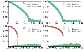
Figure 11: (Color online) Variation of order parameter $r$ with adiabatically-tuned $\sigma$ in the stationary state of the dynamics (5) on a lattice of size $L=3200$ and for four values of $K$, namely, $K=0.04$ (panel (a)), $K=-0.1$ (panel (b)), $K=-0.23$ (panel (c)), and $K=-0.24$ (panel (d)). The frequency distribution $g(\omega)$ is a Lorentzian with zero mean and unit width. The results correspond to a typical realization of the frequencies. Hysteresis behaviour is observed only in panels (c) and (d). The data are obtained from numerical integration of the dynamics (5).

VI Conclusions

In this work, we studied a variation of the celebrated Kuramoto model of spontaneous collective synchronization, by including in the dynamics a nearest-neighbor interaction on a one-dimensional lattice with periodic boundary conditions. For unimodal and symmetric frequency distributions, we demonstrated that the resulting dynamics exhibits a rich phase diagram in the stationary state, with the system exhibiting synchronized and incoherent phases separated by transition lines that could be either continuous or first-order. The first-order and continuous transition lines meet at a tricritical point. For such frequency distributions, the usual Kuramoto model that has only mean-field interaction exhibits continuous transitions and the model with solely nearest-neighbor interactions exhibits the incoherent phase with no transitions. Our work highlights that a competition between the two types of interactions brings in new features, namely, that the system in contrast to the only-nearest-neighbor case does exhibit global synchrony, and moreover, that transitions between the synchronized and the incoherent phase can be either continuous or first-order depending on parameter regimes. Although we have studied in detail the case of Gaussian frequency distributions, we have verified for another choice of the distribution, namely, a Lorentzian, the existence of continuous and first-order transitions, see Fig. 11. In the light of the results presented here in the context of the model (1) that is a special case of the dynamics (37) discussed in Appendix A, it would be interesting to study the phase diagram of the latter model that is more general. Investigations in these directions will be reported elsewhere.

Appendix A Motivating the form of the dynamics (1)

The dynamics (1) may be motivated from a completely different perspective than that of coupled oscillators, which serves to rationalize the physical setting of the model. To this end, consider a system of interacting rotors occupying the sites of a one-dimensional periodic lattice of $L$ sites, with sites labeled $i=1,2,\ldots,L$. Let $(\theta_{i},p_{i})$ be the canonically-conjugate variables for the $i$-th rotor; here, the angle $\theta_{i}\in[0,2\pi)$, with $\theta_{i+L}=\theta_{i}$, is the generalized coordinate, while $p_{i}$ is the corresponding conjugate momentum. The Hamiltonian of the system is given by Campa et al. (2006); Dauxois et al. (2010); Campa et al. (2014)

$$H=\sum_{i=1}^{L}\frac{p_{i}^{2}}{2I}+\frac{J}{2L}\sum_{i,j=1}^{L}\left[1-\cos(\theta_{i}-\theta_{j})\right]$$

$$~{}~{}~{}~{}~{}~{}~{}~{}~{}~{}~{}~{}~{}~{}-K\sum_{i=1}^{L}[\cos(\theta_{i+1}-\theta_{i})+\cos(\theta_{i-1}-\theta_{i})],$$ (32)

which models two kinds of interactions between the rotors: a nearest-neighbor interaction with coupling $K$ that can be either positive or negative, and a mean-field ferromagnetic interaction with coupling $J>0$. Here, $I$ is the common moment of inertia of the rotors. The model (32) naturally arises in the context of a class of layered magnets (such as $\mathrm{(CH_{3}NH_{3})_{2}CuCl_{4}}$) that in specific temperature ranges and for certain sample shapes is faithfully described by a microscopic Hamiltonian reducible to a Hamiltonian of classical rotators on a one-dimensional lattice with both a nearest-neighbor and a mean-field interaction, namely, of the form (32), see Refs. Sato and Sievers (2004); Wrubel et al. (2005); Sato and Sievers (2005); Dauxois et al. (2010). Such a reduction is supposed to be generic for systems dominated by dipolar forces Dauxois et al. (2009); Landau and Lifshitz (1960), and so the Hamiltonian (32) is not just a model of academic interest but is strongly grounded in the physics of layered magnetic structures.

The dynamics of the system (32) is generated by the Hamilton’s equations of motion derived from the Hamiltonian (32), as

$$\frac{{\rm d}\theta_{i}}{{\rm d}t}=\frac{p_{i}}{I},$$

$$\frac{{\rm d}p_{i}}{{\rm d}t}=\frac{J}{L}\sum_{j=1}^{L}\sin(\theta_{j}-\theta_{i})+K\sum_{j\in nn_{i}}\sin(\theta_{j}-\theta_{i}).$$ (33)

With $K=0$, the model (32) reduces to a paradigmatic model of long-range interactions, the so-called Hamiltonian mean-field (HMF) model, which has been extensively studied over the years to exemplify a number of peculiar static and dynamic properties exhibited by long-range interacting systems Campa et al. (2014). The dynamics (33) conserves total energy of the system and as such models time evolution within a microcanonical ensemble. In order to mimic the interaction of the system with the external environment modeled as a heat bath at a constant temperature $T$, one introduces in the spirit of Langevin dynamics a suitable friction term in the dynamics resulting in the following time evolution within a canonical ensemble:

$$\frac{{\rm d}\theta_{i}}{{\rm d}t}=\frac{p_{i}}{I},$$

(34)

$$\frac{{\rm d}p_{i}}{{\rm d}t}=-\gamma\frac{p_{i}}{I}+\frac{J}{L}\sum_{j=1}^{L}\sin(\theta_{j}-\theta_{i})+K\sum_{j\in nn_{i}}\sin(\theta_{j}-\theta_{i})+\eta_{i}(t).$$

Here, $\gamma>0$ is the friction constant, while $\eta_{i}(t)$ is a Gaussian, white noise with properties

$$\langle\eta_{i}(t)\rangle=0,~{}~{}\langle\eta_{i}(t)\eta_{j}(t^{\prime})\rangle=2\gamma k_{B}T\delta_{ij}\delta(t-t^{\prime}),$$ (35)

where angular brackets denote averaging with respect to noise realizations, and $k_{B}$ is the Boltzmann constant.

From the form of the Hamiltonian (32), it is clear that the interaction terms may induce (depending on the relative magnitudes of $J$ and $K$) a clustering of rotor angles and consequently a macroscopic order in the system. It is then natural to define the so-called (complex) magnetization order parameter

$$me^{{\rm i}\psi}\equiv\frac{1}{L}\sum_{j=1}^{L}e^{{\rm i}\theta_{j}},$$ (36)

with $m$ denoting the magnetization or the amount of clustering present in the system at any time instant. Both the dynamics (33) and (34) allow a stationary state that is an equilibrium one, namely, microcanonical equilibrium for the former and canonical equilibrium for the latter. The phase diagram of the model in both microcanonical and canonical equilibrium has been studied in the past, and it has been found that the model with $K=0$ exhibits a continuous phase transition between a magnetized ($m\neq 0$) and a non-magnetized ($m=0$) phase at the critical temperature $k_{B}T_{c}=J/2$ in canonical equilibrium and at the corresponding critical energy $\epsilon_{c}=3J/4$ in microcanonical equilibrium. With $K\neq 0$, the model exhibits a very rich phase diagram with both first-order and continuous phase transitions and a tricritical point Campa et al. (2006); Dauxois et al. (2010).

Being rotors, it is natural that they may be subject to external torques that vary from one rotor to the other. To model this situation, we may modify the dynamics (34) to read

$$\frac{{\rm d}\theta_{i}}{{\rm d}t}=\frac{p_{i}}{I},$$

(37)

$$\frac{{\rm d}p_{i}}{{\rm d}t}=\omega_{i}-\gamma\frac{p_{i}}{I}+\frac{J}{L}\sum_{j=1}^{L}\sin(\theta_{j}-\theta_{i})$$

$$~{}~{}~{}~{}~{}~{}~{}~{}~{}~{}~{}~{}+K\sum_{j\in nn_{i}}\sin(\theta_{j}-\theta_{i})+\eta_{i}(t),$$

where $\omega_{i}$ is a quenched random variable denoting the external torque acting on the $i$-th rotor. We may consider all the $\omega_{i}$’s to be sampled from a common distribution. The dynamics (37) does not derive from an underlying Hamiltonian, since the presence of $\omega_{i}$’s does not allow an interparticle potential to be defined that is periodic in the $\theta_{i}$’s (see the discussion preceding Eq. (4)), and this is but natural as the $\omega_{i}$’s represent after all torques applied externally to the system. An immediate consequence is that the dynamics (37) has a stationary state that is generically a nonequilibrium one, in contrast to the case with $\omega_{i}=0~{}\forall~{}i$ when as argued above the stationary state is an equilibrium one. As opposed to equilibrium stationary states that are time-reversal invariant, encoded in the so-called principle of detailed balance that such states satisfy, nonequilibrium stationary states (NESSs) manifestly violate detailed balance leading to nonzero loops of probability current in the configuration space, and offer an active area of research in the arena of modern day statistical mechanics Livi and Politi (2017). Unlike equilibrium states that may all be characterized in terms of the well-founded Gibbs-Boltzmann ensemble theory encompassing microcanonical and canonical ensembles, a general tractable framework built in the same vein that allows to study NESSs on a common footing is as yet lacking, implying that NESSs need to be studied on a case-by-case basis. It is then evidently of interest to study model systems with NESSs which are simple enough to allow for detailed analytical characterization and yet are general enough to capture the essential features of observed physical phenomena.

Now, we may imagine a situation in which the friction constant has such a high value that the ration $I/\gamma\to 0$, and the dynamics (37) needs to be considered in the overdamped limit. The resulting dynamics in this limit is obtained from Eq. (37) as

$$\gamma\frac{{\rm d}\theta_{i}}{{\rm d}t}=\omega_{i}+\frac{J}{L}\sum_{j=1}^{L}\sin(\theta_{j}-\theta_{i})+K\sum_{j\in nn_{i}}\sin(\theta_{j}-\theta_{i})+\eta_{i}(t).$$ (38)

Dividing throughout by $\gamma$, and redefining the couplings as $J/\gamma\to J$, $K/\gamma\to K$ and the torque as $\omega_{i}\to\omega_{i}/\gamma$, one obtains

$$\frac{{\rm d}\theta_{i}}{{\rm d}t}=\omega_{i}+\frac{J}{L}\sum_{j=1}^{L}\sin(\theta_{j}-\theta_{i})+K\sum_{j\in nn_{i}}\sin(\theta_{j}-\theta_{i})+\zeta_{i}(t),$$ (39)

where $\zeta_{i}(t)\equiv\eta_{i}(t)/\gamma$ satisfies $\langle\zeta_{i}(t)\rangle=0,~{}\langle\zeta_{i}(t)\zeta_{j}(t^{\prime})\rangle=(2k_{B}T/\gamma)\delta_{ij}\delta(t-t^{\prime})$. Noting that the magnetization order parameter (36) is exactly identical to the Kuramoto synchronization order parameter (2), the dynamics (39) may be rewritten in terms of the quantities $r$ and $\psi$, as

$$\frac{{\rm d}\theta_{i}}{{\rm d}t}=\omega_{i}+Jr\sin(\psi-\theta_{i})+K\sum_{j\in nn_{i}}\sin(\theta_{j}-\theta_{i})+\zeta_{i}(t).$$ (40)

It is then evident that the dynamics (1) is a special case of the dynamics (40) with $T$ set to zero. We have thus provided a concrete rationale for the model (1) from a perspective other than that of Kuramoto oscillators.

Appendix B Scaling theory of continuous transitions in equilibrium

Equilibrium continuous phase transitions are associated with a singularity in the second derivative of the free energy, and are observed strictly in an infinite system Fisher (1967). While the limit of an infinite system can be achieved in theoretical analysis, experiments and numerical analysis invariably involve systems of finite size. Finite-size scaling theory allows to estimate the phase transition point, i.e., the parameter value at which a singularity occurs in an infinite system, by analyzing the data for large but finite systems. For our discussions of the finite-size scaling theory, consider a system with two different phases characterized by a real scalar order parameter $\Psi$, and a continuous phase transition occurring as a function of temperature $T$ with the system existing in an ordered phase with $|\Psi|>0$ (respectively, in a disordered phase with $\Psi=0$) at temperatures below a critical temperature $T_{c}$ (respectively, at and above $T_{c}$). Defining $t\equiv(T-T_{c})/T_{c}$ and considering a system with linear dimension $L$ (so that $N$, the number of degrees of freedom, scales as $N\sim L^{d}$, with $d$ being the dimension of the embedding space), let us denote the correlation length as $\xi(L)$, the order parameter as $\Psi(L)$, and consider the quantity $\chi(L)\equiv L^{d}\left(\langle(\Psi(L))^{2}\rangle-\langle\Psi(L)\rangle^{2}\right)$, measuring stationary-state fluctuations of the order parameter and related to the zero-field susceptibility. Here, $\langle\cdot\rangle$ denotes time average in the stationary state. Then, a continuous phase transition, observed as $L\to\infty$, is characterized by the divergence of the correlation length $\xi(\infty)$ at temperatures around the critical point as $\xi(\infty)\sim|t|^{-\nu};~{}t\to 0$, where $\nu$ is a critical exponent Fisher (1967). The critical exponent $\beta$ characterizes the behavior of $\Psi(\infty)$ close to the critical point, as $\Psi(\infty)\sim(-t)^{\beta};~{}t\to 0^{-}$. The quantity $\chi(\infty)$ is on the other hand known to diverge as $\chi(\infty)\sim|t|^{-\gamma};~{}t\to 0$, where $\gamma$ is another critical exponent. For large but finite $L$ and at a given $|t|\to 0$, if one has $L\gg\xi(\infty)$, no significant finite-size effects should be observed. On the other hand, for $L\ll\xi(\infty)$, the system size will cut-off long-distance correlations, and hence, finite-size rounding off of critical-point singularities is expected. It is then reasonable to expect for small $|t|$ that the ratio $\xi(\infty)/L$ (or, equivalently, the ratio $|t|L^{1/\nu}$) controls the behavior of $\chi,~{}\Psi$, etc, so that one may write under the assumptions of the finite-size scaling theory the following scaling forms Landau and Binder (2009):

$$\Psi(L)\sim L^{-\beta/\nu}f(|t|L^{1/\nu}),$$

(41)

$$\chi(L)\sim L^{\gamma/\nu}g(|t|L^{1/\nu}).$$

The scaling functions $f(x)$ and $g(x)$, defined with $x>0$, behave in the limit $x\to\infty$ as $f(x)\sim x^{\beta}$ and $g(x)\sim x^{-\gamma}$. In the limit $x\to 0$, the functions behave as $f(x)|_{x\to 0}\to$ constant and $g(x)|_{x\to 0}\to$ constant. Such forms ensure that as required, in the limit $L\to\infty$ at a fixed and small $|t|$, we have $\Psi(\infty)\sim t^{\beta}$ and $\chi(\infty)\sim|t|^{-\gamma}$. On the other hand, at a fixed $L$, as $|t|\to 0$, one has $\Psi(L)\sim L^{-\beta/\nu}$ and $\chi(L)\sim L^{\gamma/\nu}$.

In order to estimate the critical point of a continuous transition, one proceeds as follows. For finite $L$, the infinite-$L$ divergence in $\chi$ is rounded and shifted over a finite range of temperature around a pseudo-critical point $T_{c}(L)$; in the limit $L\to\infty$, the region shrinks to zero and $T_{c}(L)$ converges to infinite-$L$ value $T_{c}$ as Binder

$$T_{c}(L)-T_{c}\propto L^{-1/\lambda_{T}},$$ (42)

with $\lambda_{T}$ a phenomenological exponent to characterize the shifting of $T_{c}(L)$ with $L$. In numerics, one uses the data for the maximum of $\chi(L)$ for different $L$ to obtain $T_{c}(L)$ as a function of $L$. Fitting the plot to a power law of the form (42) then allows to estimate $T_{c}$. Using this value of $T_{c}$ and the scaling forms (41), one then plots the finite-$L$ data ($L^{\beta/\nu}\Psi(L)$ vs. $|t|L^{1/\nu}$ and $L^{-\gamma/\nu}\chi(L)$ vs. $|t|L^{1/\nu}$) and obtains estimates of the critical exponents by requiring that the data for large $L$ collapse onto each other.