Multi-Node EM Algorithm for Finite Mixture Models

Abstract

Finite mixture models are powerful tools for modelling and analyzing heterogeneous data. Parameter estimation is typically carried out using maximum likelihood estimation via the Expectation-Maximization (EM) algorithm. Recently, the adoption of flexible distributions as component densities has become increasingly popular. Often, the EM algorithm for these models involves complicated expressions that are time-consuming to evaluate numerically. In this paper, we describe a parallel implementation of the EM-algorithm suitable for both single-threaded and multi-threaded processors and for both single machine and multiple-node systems. Numerical experiments are performed to demonstrate the potential performance gain in different settings. Comparison is also made across two commonly used platforms - R and MATLAB. For illustration, a fairly general mixture model is used in the comparison.

1 Introduction

In recent years there has been an increasing use of finite mixtures of flexible distributions for the modelling and analysis of heterogeneous and non-normal data McLachlan et al. (2019). These models adopt component densities that offer a high degree of flexibility in distributional shapes. In particular, the skew-symmetric family of distributions, which includes the classical skew normal and skew $t$-distributions, has become increasingly popular Wang et al. (2009), Lin (2010), Frühwirth-Schnatter and Pyne (2010), Cabral et al. (2012), Lin et al. (2014), Lee and McLachlan (2016). It has enjoyed applications in a range of areas including astrophysics, bioinformatics, biology, climatology, medicine, finance, fisheries, and social sciences Riggi and Ingrassia (2013), Allard and Soubeyrand (2012), Tagle et al. (2019), Pyne et al. (2009), Lee et al. (2016b), Hejblum et al. (2019), Contreras-Reyes and Arellano-Valle (2013), Asparouhov and Muthén (2015), Hohmann et al. (2018).

Traditionally, finite mixture models are fitted by maximum likelihood estimation, carried out via the Expectation-Maximization (EM) algorithm Dempster et al. (1977). For simple component densities like the normal and $t$-distributions, the E- and M-steps are usually quite straightforward. But for some flexible distributions such as the skew normal and skew-$t$ mixture models, the E-step often involves complicated expressions; see the aforementioned references. For example, the conditional expectations in the E-step may require calculation of the moments of truncated (multivariate) distributions. Depending on the particular characterization of the component densities, this may involve numerical evaluations of multidimensional integrals that are computationally demanding.

To speed up the model fitting process, a number of recent works have presented modified versions of the EM algorithm for parallel computing. The vast majority of these contributions are aimed at large scale distributed and/or cloud platforms such as GraphLab, Piccolo, and Spark; see, for example Low et al. (2012), Gonzalez et al. (2012), Power and Li (2010), Li et al. (2011), Zaharia et al. (2010). Relatively few have focused on smaller scale environments with a single machine or a small local network of machines. The paper Lee et al. (2016a) presented a simple parallel version of the EM algorithm for single machine, taking advantage of multithreading. For a $g$-component mixture model, the authors proposed to split the computations across $g$ threads. We shall refer to this as the multi-EM algorithm. The advantage of this approach is its simplicity and ease of implementation, as it requires minimal modification to the original (serial) code. More recently, Lee et al. (2019) presented a block EM algorithm where the data are horizontally split into $b$ blocks, allowing for an arbitrary number of threads to be used. Their algorithm was illustrated on multi-core machines. Note that both the multi-EM and block-EM algorithms were implemented in R and aimed at single (standalone) machines.

In this paper, we describe another parallel implementation of the EM algorithm that is suitable for both single and small networks of machines. The structure of the EM algorithm allows easy splitting of the E-step into a single thread for each single observation and component. The M-step can also be naturally split into $g$ separate threads. Depending on the physical system used, the user may choose an appropriate number of threads to use for the E- and M-steps. For illustration, we adopt the finite mixture of canonical fundamental skew $t$ (CFUST) distributions Arellano-Valle and Genton (2005) to assess the performance of the parallel algorithms. In addition, we implemented the algorithms in two commonly used mathematical platforms, namely R and MATLAB, and compared the performance gain across these platforms.

2 The EM algorithm for finite mixture models

Finite mixture models provide a convenient mathematical representation of heterogeneous clusters within the data. Formally, the density of a finite mixture model is a convex combination of component densities. Let $Y$ denotes a $p$-dimensional random vector consisting of $p$ feature variables of interest, and $y$ be a realization of $Y$. Then the density of a $g$-component mixture model takes the form

$$f(\mbox{\boldmath$y$};\mbox{\boldmath$\Psi$}) = \sum_{i=1}^{g}\pi_{i}f_{i}(\mbox{\boldmath$y$};\mbox{\boldmath$\theta$}_{i}),$$ (1)

where $\pi_{i}$ denotes the mixing proportion for component $i$, $f_{i}(\cdot)$ denotes the density of the $i$th component of the mixture model, and $\mbox{\boldmath$\theta$}_{i}$ denotes the vector of unknown parameters of the $i$th component, for $i=1,2,\ldots,g$. The vector $\Psi$ contains all the unknown parameters of the mixture model, that is, $\mbox{\boldmath$\Psi$}=(\pi_{1},\ldots,\pi_{g-1},\mbox{\boldmath$\theta$}_{1}^{\top},\ldots,\mbox{\boldmath$\theta$}_{g}^{\top})$. Note that the mixing proportions satisfy $\pi_{i}>0$ and $\sum_{i=1}^{g}\pi_{i}=1$.

Traditionally, the component density is taken to be the (multivariate) normal distribution, that is, $f_{i}(\cdot)=\phi_{p}(\mbox{\boldmath$y$};\mbox{\boldmath$\mu$},\mbox{\boldmath$\Sigma$})$ where $\mu$ is a $p$-dimensional vector of location parameters and $\Sigma$ is a positive-definite scale matrix. For illustration purposes, we consider $f_{i}(\cdot)$ to be the CFUST density in this paper, which is given by

$$f_{\mbox{\tiny{CFUST}}}(\mbox{\boldmath$y$};\mbox{\boldmath$\mu$},\mbox{\boldmath$\Sigma$},\mbox{\boldmath$\Delta$},\nu)=2^{q}\,t_{p}(\mbox{\boldmath$y$};\mbox{\boldmath$\mu$},\mbox{\boldmath$\Omega$},\nu)\,T_{q}\left(\mbox{\boldmath$\delta$}^{\top}\mbox{\boldmath$\Omega$}^{-1}(\mbox{\boldmath$y$}-\mbox{\boldmath$\mu$})\sqrt{\frac{\nu+p}{\nu+d(\mbox{\boldmath$y$})}};\mbox{\boldmath$0$},\mbox{\boldmath$\Lambda$},\nu+p\right),$$ (2)

where $t_{p}(\cdot)$ denotes the $p$-dimensional $t$-density and $T_{p}(\cdot)$ denote its corresponding cumulative distribution function. In the above, we let $\mbox{\boldmath$\Omega$}=\mbox{\boldmath$\Sigma$}+\mbox{\boldmath$\Delta$}\mbox{\boldmath$\Delta$}^{\top}$, $\mbox{\boldmath$\Lambda$}=\mbox{\boldmath$I$}_{q}-\mbox{\boldmath$\Delta$}^{\top}\mbox{\boldmath$\Omega$}^{-1}\mbox{\boldmath$\Delta$}$, and $d(\mbox{\boldmath$y$})=(\mbox{\boldmath$y$}-\mbox{\boldmath$\mu$})^{\top}\mbox{\boldmath$\Omega$}^{-1}(\mbox{\boldmath$y$}-\mbox{\boldmath$\mu$})$ is the Mahalanobis distance between $y$ and $\mu$. We shall refer to finite mixtures of (2) as FM-CFUST. The CFUST distribution is fairly flexible and contains, as special and/or limiting cases, many commonly used distributions including the normal, $t$, Cauchy, and skew normal distributions. These are obtained by letting $\mbox{\boldmath$\Delta$}=\mbox{\boldmath$0$}$ and $\nu\to\infty$; $\mbox{\boldmath$\Delta$}=\mbox{\boldmath$0$}$; $\mbox{\boldmath$\Delta$}=\mbox{\boldmath$0$}$ and $\nu=1$; and $\nu\to\infty$, respectively. In addition, several characterizations of skew normal and skew $t$-distributions are also special and/or limiting cases of (2) Lee and McLachlan (2013).

Estimation of $\Psi$ for mixture models is typically undertaken by maximum likelihood via the EM algorithm. The EM algorithm begins with an initialization step, where an initial estimate $\mbox{\boldmath$\Psi$}^{(0)}$ of $\Psi$ are computed from an initial partition or via other strategies. We then alternate the E- and M-steps until some stopping criterion is satisfied. To facilitate parameter estimation via the EM algorithm, a set of latent binary variables $\mbox{\boldmath$Z$}_{j}$ is introduced, representing the component membership of $\mbox{\boldmath$y$}_{j}$ – the $j$th observation in the data. More formally, $Z_{ij}=(Z_{j})_{i}=1$ if $\mbox{\boldmath$y$}_{j}$ belongs to the $i$th component of the mixture model and zero otherwise. Depending on the choice of the component density, additional latent variables may be introduced to simplify calculations. In the case of FM-CFUST, these include latent gamma random variables and latent truncated normal random variables. The technical details of the EM algorithm for FM-CFUST are omitted here, but can be found in Lee and McLachlan (2016). An outline of the procedure of the EM algorithm is given below.

1. Initialization: Obtain $\mbox{\boldmath$\Psi$}^{(0)}$ from an initial partition or some other starting strategies. Calculate the initial log likelihood value using the following with $k=0$:

   $$\ell^{(k)}=\sum_{j=1}^{n}\log f(\mbox{\boldmath$y$}_{j};\mbox{\boldmath$\Psi$}^{(k)}).$$ (3)

2. E-step: Calculate the posterior probability of component membership:

   $$\tau_{ij}^{(k)}=\frac{\pi_{i}^{(k)}f_{i}(\mbox{\boldmath$y$}_{j};\mbox{\boldmath$\theta$}_{i}^{(k)})}{f(\mbox{\boldmath$y$}_{j};\mbox{\boldmath$\Psi$}^{(k)})}=\frac{f_{ij}^{(k)}}{f_{j}^{(k)}},$$ (4)

   for $i=1,2,\ldots,g$ and $j=1,2,\ldots,n$. Calculate any other required conditional expectations $\mbox{\boldmath$e$}_{1ij}^{(k)}$, $\mbox{\boldmath$e$}_{2ij}^{(k)},\ldots$.

3. M-step: Compute updated parameter estimates $\mbox{\boldmath$\Psi$}^{(k+1)}$ based on the output of the E-step.

4. Stopping criterion: Update the log likelihood value using (3). Check whether the stopping criterion is satisfied. If so, return the output of the M-step. Otherwise, increment $k$ to $k+1$ and return to the E-step.

3 A multi-node EM algorithm

The computation of the conditional expectations in the E-step can be quite time consuming, especially for large values of $p$ (and $q$ in the case of FM-CFUST). We now describe a parallel implementation of the EM algorithm that is suitable for multi-core and/or multi-node operating systems. As can be observed from the structure of the EM algorithm outlined above, the computation of $\tau_{ij}^{(k)}$ and other conditional expectations in the E-step can be carried out separately for each $i$ and $j$. It is thus intuitive to split the data into $m$ blocks where $1\leq m\leq gn$. The value of $m$ can be user-specified or chosen to best match the physical systems. In R, $m$ needs to be specified explicitly, whereas for MATLAB $m$ will be set to the number of physical cores in the system by default. Note that the system may comprise of more than one machine and thus $m$ is the total number of physical cores across all machines.

3.1 Parallel initialization

The EM algorithm is sensitive to starting values and thus it is important to choose good initial estimates for the parameters of the model. With $m$ threads, we can trial $m$ different initializations concurrently. The algorithm begins with $m$ different initial partitions that can be obtained, for example, by $k$-means or random partitions. Each of the $m$ threads computes $\mbox{\boldmath$\Psi$}^{(0)}$ based on the given initial partition. The initial log likelihood value $\ell^{(0)}$ is then computed. There is an option for each thread to compute a small number $r$ of (burn-in) EM iterations. However, for simplicity we have used $r=0$ in the numerical experiments, that is, without any burn-in iterations. A master thread then gathers the $\ell^{(0)}$ from the $m$ threads and selects the one with the smallest value of $\ell^{(0)}$ to provide the starting values for the multi-node EM algorithm.

In the process of computing $\ell^{(k)}$, the quantities $f_{ij}^{(k)}$ and hence $f_{j}^{(k)}$ (4), were evaluated for $i=1,2,\ldots,g$ and $j=1,2,\ldots,n$. They correspond to the numerator and denominator of $\tau_{ij}^{(k)}$, respectively. Hence, the $\tau_{ij}^{(1)}=f_{ij}^{(0)}/f_{j}^{(0)}$ are also computed during the initialization step and are passed on to the E-step in the first iteration. A summary of the parallel initialization step is presented in Algorithm 1.

Algorithm 1 Parallel initialization step of multi-node EM algorithm

1:Compute $m$ different initial partitions of the data.

2:for thread $l\in\{1,2,\ldots,m\}$ do concurrently

3:     Compute $\mbox{\boldmath$\Psi$}^{(0)}$.

4:     Compute $f_{ij}^{(0)}$ for $i=1,2\ldots,g$ and $j=1,2,\ldots,n$.

5:     Calculate $f_{j}^{(0)}=\sum_{i=1}^{n}\pi_{i}^{(0)}f_{ij}^{(0)}$.

6:     Calculate $\ell^{(0)}=\sum_{j=1}^{n}\log f_{j}^{(0)}$.

7:     Calculate $\tau_{ij}^{(1)}=f_{ij}^{(0)}/f_{j}^{(0)}$.

8:     (Optional) Run $r$ iterations of the EM algorithm.

9:     Return $\ell^{(0)}$, $\mbox{\boldmath$\Psi$}^{(0)}$, and $\tau_{ij}^{(1)}$ to the master thread.

10:end for

11:Select $l$ that corresponds to the smallest $\ell^{(0)}$ from the results of the $m$ threads.

12:Return the selected $\ell^{(0)}$, $\mbox{\boldmath$\Psi$}^{(0)}$, and $\tau_{ij}^{(1)}$.

3.2 Parallel E-step

Computation of the conditional expectations $\mbox{\boldmath$e$}_{1ij}^{(k)},\mbox{\boldmath$e$}_{2ij}^{(k)},\ldots$ can be performed in parallel for each $i$ and $j$. Depending on the total number of threads, if $m<ng$ then a thread $l$ may be responsible for more than one value of $i$ and $j$. For performance, preference would be given to $i$ so that $\tau_{ij}^{(k)}$ can be computed in the same thread for each $j$. Let $l=1,2,\ldots,m$ be the index of the threads and $J_{l}$ be the set of index (of observations) assigned to thread $l$. An outline of the E-step is presented in Algorithm 2. During the E-step, each thread calculates $\tau_{ij}^{(k)}$, $\ell_{l}^{(k-1)}$, and $\mbox{\boldmath$e$}_{1ij}^{(k)},\mbox{\boldmath$e$}_{2ij}^{(k)},\ldots$ for observations $\mbox{\boldmath$y$}_{j}$ in $i\in J_{l}$. For the first iteration, $\tau_{ij}^{(1)}$ have been passed on from the initialization step and hence can be skipped. Unlike the traditional implementation of the EM-algorithm, we also compute partial sums of conditional expectations that will be required in the M-step. These are denoted by $s_{1il}^{(k)}=\sum_{j\in J_{l}}\tau_{ij}^{(k)}$, $\mbox{\boldmath$s$}_{2il}^{(k)}$, etc. The expression for these partial sums depend on the component density. In the case of the FM-CFUST model, the eight partial sums are given by equations (27) to (34) in Lee et al. (2019).

Algorithm 2 Parallel E-step of multi-node EM algorithm

1:for thread $l\in\{1,2,\ldots,m\}$ do concurrently

2:     for $j\in J_{1}$ do

3:         if k¿1 then for $i\in\{1,2,\ldots,g\}$

4:              Compute $f_{ij}^{(k-1)}$.

5:              Calculate $f_{j}^{(k-1)}=\sum_{i=1}^{n}\pi_{i}^{(k-1)}f_{ij}^{(k-1)}$.

6:              Calculate $\tau_{ij}^{(k)}=f_{ij}^{(k-1)}/f_{j}^{(k-1)}$.

7:              Calculate $\ell_{l}^{(k-1)}=\sum_{j=1}^{n}\log f_{j}^{(k-1)}$.

8:         end if

9:         Compute conditional expectations $\mbox{\boldmath$e$}_{1ij}^{(k)},\mbox{\boldmath$e$}_{2ij}^{(k)},\ldots$.

10:         Compute partial sums $s_{1il}^{(k)},\mbox{\boldmath$s$}_{2il}^{(k)},\ldots$

11:         Return conditional expectations and partial sums to the master thread.

12:     end for

13:end for

3.3 Parallel M-step

The M-step can be inherently separated into $g$ threads. It is also possible to split into a larger number of threads by separately the calculations of each component of $\mbox{\boldmath$\Psi$}_{i}^{(k)}$ into a number of threads. However, given that the M-step expressions are often relatively inexpensive to evaluate, it may be preferable for all components of $\mbox{\boldmath$\Psi$}_{i}^{(k)}$ to be computed by the same thread. While the $g$ threads are computing $\mbox{\boldmath$\Psi$}_{i}^{(k)}$ simultaneously, the master thread computes $\ell^{(k-1)}$ by calculating the summation of $\ell_{l}^{(k-1)}$ returned by the $l$ threads after the parallel E-step. Once the calculation of $\mbox{\boldmath$\Psi$}_{i}^{(k)}$ is completed by the $g$ parallel threads, these can be combined into $\mbox{\boldmath$\Psi$}^{(k)}$ by the master thread. A summary of the parallel M-step of the multi-node EM algorithm is presented in Algorithm 3.

Algorithm 3 Parallel M-step of multi-node EM algorithm

Split the E-step results from $l$ threads by component

1:for thread $i\in\{1,2,\ldots,g\}$ do concurrently

2:     Compute $\mbox{\boldmath$\Psi$}_{i}^{(k)}$ using $\mbox{\boldmath$e$}_{1ij}^{(k)},\mbox{\boldmath$e$}_{2ij}^{(k)},\ldots$.

3:     Return $\mbox{\boldmath$\Psi$}_{i}^{(k)}$ to master thread.

4:end for

5:Compute $\ell^{(k-1)}=\sum_{l=1}^{m}\ell_{l}^{(k-1)}$.

6:Combine $\mbox{\boldmath$\Psi$}_{i}^{(k)}$ into $\mbox{\boldmath$\Psi$}^{(k)}$.

3.4 Stopping criterion

We adopt the Aitken acceleration-based stopping criterion to determine whether the EM algorithm can be stopped after the $k$th iteration. The details are given in Algorithm 4. It can be observed from Algorithm 4 that the calculations are rather simple and hence can be performed by a single thread (that is, the master thread).

Algorithm 4 Stopping criterion for multi-node EM algorithm

1:Calculate Aitken’s acceleration $a^{(k-1)}=\frac{\ell^{(k)}-\ell^{(k-1)}}{\ell^{(k-1)}-\ell^{(k-2)}}$.

2:Calculate $\ell_{\infty}^{(k)}=\ell^{(k-1)}+\frac{\ell^{(k)}-\ell^{(k)}}{1+a^{(k-1)}}$.

3:if $|\ell_{\infty}^{(k)}-\ell^{(k)}|<\epsilon$ then

4:     Return $\mbox{\boldmath$\Psi$}^{(k)}$ and $\ell^{(k-1)}$.

5:     Terminate the algorithm.

6:end if

7:Set $k$ to $k+1$.

8:Return to Algorithm 2.

4 Numerical experiments

We performed numerical experiments to assess the performance of the multi-node EM algorithm under three different physical settings. The algorithm was implemented using both R and MATLAB and executed on machine(s) running Windows. The machine(s) have four physical cores. For the R implementation, the parallel package that is available in base R was used. For the MATLAB implementation, the Parallel Computing Toolbox was used. For a fair comparison between MATLAB and R, efforts have been made so that the R and MATLAB codes are almost direct transcriptions of each other. For example, the same set of commands were implemented for the computation of (multivariate) truncated moments. For illustration, the algorithm was implemented for the FM-CFUST model and applied to the Australian Institute of Sport (AIS) data Cook and Weisberg (1994). The AIS data comprises $p=11$ body measurements on $n=202$ athletes. We apply the clustering algorithms to predict the gender of each athlete. For consistency, the same set of initial partitions was used and the number of components were fixed at $g=2$. The three settings for parallel computing are listed below.

1. single-threaded: using a single thread on a CPU core on a single machine

2. multi-threaded: using 2 to $12$ threaded on a single machine. Note that the threads may be virtual threads.

3. multi-node: using multiple threads from two or more machines connected through a local network.

For each of the above setting, the MATLAB and R implementations were ran separately on the same machine(s) for 100 replications each. We note that the multi-node version can be rather complicated to setup in R. As such, for the multi-node setting, we focus on the MATLAB implementation.

As our main interest is the performance gain of the multi-node EM algorithm, details of the accuracy of the estimates and the clustering performance will not be reported here. However, we noted that the parameter estimates are almost identical to that obtained from the traditional (non-parallel) implementation, and all trials yielded the same final clustering.

4.1 MATLAB versus R in single-threaded implementation

The single-threaded version of the multi-node EM algorithm corresponds to the traditional implementation of the EM algorithm. This is the default setting in R and MATLAB. The mean and standard deviation (sd) of the run time for R are 2310.83 seconds and 62.04 seconds, respectively; see the third row of Table 1. For MATLAB, the mean run time of the 100 trials are 2635.69 seconds, with sd being 142.63 seconds. On average, MATLAB appears to be slightly slower than R (approximately $14\%$) in this case. These results can be used as baseline measurements for comparison with multi-threaded and multi-node implementations.

4.2 MATLAB versus R in multi-threaded implementation

With the multi-core/muti-threaded implementation, we would expect the computation to reduce as the number of threads increases. But linear reduction in $m$ should not expected as there are overheads associated with the setting up of the parallel process. In this experiment, we considered $m$ ranging from $2$ to $20$ threads. As there are only four cores in this machine, the threads are virtual when $m>4$. The total computation time (in seconds) in each trial and setting were recorded. For $m>2$, the reduction in time (in %) against the baseline was computed using (total time in MATLAB - total time in R)/(total time in R) $\times$ 100. These results are reported in table 1 an displayed in Figure 1. As can be observed the table and figure, significant reduction in time is achieved when the parallel implementation is used. With only two threads, the total time is reduced by $49\%$ and $34\%$ for R and MATLAB, respectively. At $m=4$ (the number of physical cores), a reduction of $67\%$and $64\%$ were achieved for R and MATLAB, respectively. However, the trend of decrease in total time starts to level out at around $m=10$ threads. For R, we could observe the total time even begins to increase mildly at $m=12$, possibly due to the overhead costs. On the other hand, the trend continued to decrease for large $m$ in the case of MATLAB. Although MATLAB implementation was slightly slower than the R implementation for small number of threads, it became faster than R for $m\geq 15$.

In Figure 1, the shaded region around each line is a representation of the standard deviation across the 100 trials in each setting. These trials indicate that the computation time for MATLAB seems to be more stable than R. This can also be gauged visually from the top panel of Figure 1, where the R (red) line has a slightly broader shaded region than the MATLAB (blue) line, especially for larger values of $m$. The visual message from the bottom panel of Figure 1 suggests that both implementations have comparable percentage reduction in time, with MATLAB slightly more efficient when the number of threads is large.

Number of threads ($m$)	R		MATLAB
	Total time (sec)	Time reduction (%)	Total time (sec)	Time reduction (%)
1	2310.82	–	2635.69	–
2	1171.65	49.30	1735.80	34.14
3	902.00	60.97	1115.17	57.69
4	756.48	67.26	952.46	63.86
5	669.72	71.02	854.23	67.59
6	623.03	73.04	768.07	70.86
7	591.08	74.42	706.83	73.18
8	570.85	75.30	664.17	74.80
9	552.47	76.09	643.54	75.58
10	539.92	76.64	625.11	76.28
11	532.29	76.97	608.86	76.90
12	544.34	76.44	594.21	77.46
13	551.34	76.14	581.34	77.94
14	565.21	75.54	568.77	78.42
15	580.05	74.90	556.78	78.88
16	593.98	74.30	545.38	79.31
17	603.16	73.90	534.20	79.73
18	609.62	73.62	523.43	80.14
19	613.66	73.44	525.70	80.05
20	615.02	73.39	516.34	80.41

Table 1: Total computation time (sec) and time reduction (%) of the R and MATLAB implementation on a single multi-core machine. The reported values are the mean and standard deviation (sd) from 100 trials for each setting of $m=1,2,\ldots,20$. The experiment applied the FM-CFUST model on the AIS data set.

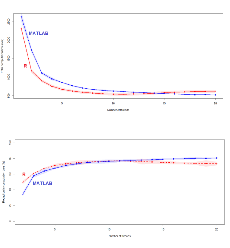
Figure 1: Performance gain of R and MATLAB implementations of the multi-node EM algorithm on the AIS data set, using $m=1,2,\ldots,20$ threads. The results for R is shown in red, whereas the results for MATLAB is shown in blue. Top panel: The circles represents the mean total computation time (seconds) across 100 trials. Shaded region around the lines indicate the standard deviation at each value of $m$. Bottom panel: The percentage reduction in time (PRT) against the baseline of $m=1$ were calculated for all cases of $m>2$. The circles represents the mean PRT across 100 trials. Shaded regions around the lines indicate the standard deviation of PRT at each value of $m$.

4.3 MATLAB multi-node implementation

For illustration, we tested the multi-node EM algorithm on a small local network of three machines with the same specifications. The number of threads is set to the total number of physical cores in the network. We recorded the total computation time of 100 trials in the case of one, two, and three machines. The results obtained by running on one machine is taken as the baseline for computing the percentage reduction in time for the case of two machines and three machines. With the multi-node setting, we would not expect a particularly good reduction in time for small data sets like in this experiment, as the high overhead associated with network communicating between the machines can overshadow the time gained by parallelizing the E- and M-steps. Indeed, we only observed a modest $2\%$ and $4.5\%$ mean reduction in time for the case of two and three machines, respectively. However, we expect these numbers to increase for larger data sets and its usefulness would be more apparent for models that are more computationally demanding.

5 Conclusions

We have described a parallel implementation of the EM algorithm for the fitting of mixture models. The multi-node EM algorithm takes advantage of parallel computing to speed up the model fitting process. Quantitative comparisons were made between the MATLAB and R implementations of the same algorithm. We find that R is a little more efficient than MATLAB, despite the latter had built-in multi-threading capabilities. For both implementations (and in the single machine setting), a significant reduction of time was observed even for small number of parallel threads. For example, the total computation time for R had reduced to almost half when only two threads were used. For big data and/or models that are more computationally demanding, the multi-node setting could provide further reduction in computation time.

References

- Allard and Soubeyrand (2012) Allard, A. and Soubeyrand, S. (2012). Skew-normality for climatic data and dispersal models for plant epidemiology: when application fields drive spatial statistics. Spatial Statistics 1, 50–64.
- Arellano-Valle and Genton (2005) Arellano-Valle, R.B. and Genton, M.G. (2005). On fundamental skew distributions. Journal of Multivariate Analysis 96, 93–116.
- Asparouhov and Muthén (2015) Asparouhov, T. and Muthén, B. (2015). Structural equation models and mixture models with continuous non-normal skewed distributions. Structural Equation Modeling .
- Cabral et al. (2012) Cabral, C.R.B., Lachos, V.H., and Prates, M.O. (2012). Multivariate mixture modeling using skew-normal independent distributions. Computational Statistics and Data Analysis 56, 126–142.
- Contreras-Reyes and Arellano-Valle (2013) Contreras-Reyes, J.E. and Arellano-Valle, R.B. (2013). Growth estimates of cardinalfish (epigonus crassicaudus) based on scale mixtures of skew-normal distributions. Fisheries Research 147, 137–144.
- Cook and Weisberg (1994) Cook, R.D. and Weisberg, S. (1994). An Introduction to Regression Graphics. New York: Wiley.
- Dempster et al. (1977) Dempster, A.P., Laird, N.M., and Rubin, D.B. (1977). Maximum likelihood from incomplete data via the EM algorithm. Journal of Royal Statistical Society B 39, 1–38.
- Frühwirth-Schnatter and Pyne (2010) Frühwirth-Schnatter, S. and Pyne, S. (2010). Bayesian inference for finite mixtures of univariate and multivariate skew-normal and skew- distributions. Biostatistics 11, 317–336.
- Gonzalez et al. (2012) Gonzalez, J.E., Low, Y., Gu, H., Bickson, D., and Guestrin, C. (2012). Powergraph: Distributed graph-parallel computation on natural graphs. In Proceedings of the 10thUSENIX Symposium on Operating Systems Design and Implementation (OSDI’12), 17–30. Hollywood, CA, USA.
- Hejblum et al. (2019) Hejblum, B.P., Alkhassim, C., Gottardo, R., Caron, F., and Thiébaut, R. (2019). Sequential dirichlet process mixtures of multivariate skew -distributions for model-based clustering of flow cytometry data. Annals of Applied Statistics 13, 638–660.
- Hohmann et al. (2018) Hohmann, L., Holtmann, J., and Eid, M. (2018). Skew mixture latent state-trait analysis: A monte carlo simulation study on statistical performance. Frontiers in Psychology 9, 1323.
- Lee et al. (2016a) Lee, S.X., Leemaqz, K.L., and McLachlan, G.J. (2016a). A simple parallel em algorithm for statistical learning via mixture models. In Proceedings of the 2016 International Conference on Digital Image Computing: Techniques and Applications, 295–302.
- Lee et al. (2019) Lee, S.X., Leemaqz, K.L., and McLachlan, G.J. (2019). A block EM algorithm for multivariate skew normal and skew -mixture models. IEEE transactions on neural networks and learning systems 29, 5581–5591.
- Lee and McLachlan (2013) Lee, S.X. and McLachlan, G.J. (2013). On mixtures of skew-normal and skew -distributions. Advances in Data Analysis and Classification 7, 241–266.
- Lee and McLachlan (2016) Lee, S.X. and McLachlan, G.J. (2016). Finite mixtures of canonical fundamental skew -distributions: The unification of the restricted and unrestricted skew -mixture models. Statistics and Computing 26, 573–589.
- Lee et al. (2016b) Lee, S.X., McLachlan, G.J., and Pyne, S. (2016b). Modelling of inter-sample variation in flow cytometric data with the Joint Clustering and Matching (JCM) procedure. Cytometry A .
- Li et al. (2011) Li, J., Mitchell, C., and Power, R. (2011). Oolong: Programming asynchronous distributed applications with triggers. In Proceedings of the 23rd ACM Symposium on Operating Systems Principles (SOSP 2011), 1–2.
- Lin (2010) Lin, T.I. (2010). Robust mixture modeling using multivariate skew- distribution. Statistics and Computing 20, 343–356.
- Lin et al. (2014) Lin, T.I., Ho, H.J., and Lee, C.R. (2014). Flexible mixture modelling using the multivariate skew--normal distribution. Statistics and Computing 24, 531–546.
- Low et al. (2012) Low, Y., Gonzalez, J., Kyrola, A., Bickson, D., Guestrin, C., and Hellerstein, J.M. (2012). Distributed graphlab: A framework for machine learning and data mining in the cloud. In Proceedings of the VLDB Endowment, vol. 5, 716–727.
- McLachlan et al. (2019) McLachlan, G.J., Lee, S.X., and Rathnayake, S.I. (2019). Finite mixture models. Annual review of statistics and its application 6, 355–378.
- Power and Li (2010) Power, R. and Li, J. (2010). Piccolo: building fast, distributed programs with partitioned tables. In Proceedings of the 9th USENIX conference on Operating systems design and implementation (OSDI’10), 1–14. Berkeley, CA, USA.
- Pyne et al. (2009) Pyne, S., Hu, X., Wang, K., Rossin, E., Lin, T.I., Maier, L.M., Baecher-Allan, C., McLachlan, G.J., Tamayo, P., Hafler, D.A., De Jager, P.L., and Mesirow, J.P. (2009). Automated high-dimensional flow cytometric data analysis. Proceedings of the National Academy of Sciences USA 106, 8519–8524.
- Riggi and Ingrassia (2013) Riggi, S. and Ingrassia, S. (2013). A model-based clustering approach for mass composition analysis of high energy cosmic rays. Astroparticle Physics 48, 86–96.
- Tagle et al. (2019) Tagle, F., Castruccio, S., Crippa, P., and Genton, M.G. (2019). A non‐gaussian spatio‐temporal model for daily wind speeds based on a multi‐variate skew‐ distribution. Journal of Time Series Analysis 40, 312–326.
- Wang et al. (2009) Wang, K., Ng, S.K., and McLachlan, G.J. (2009). Multivariate skew mixture models: applications to fluorescence-activated cell sorting data. In Proceedings of Conference of Digital Image Computing: Techniques and Applications, H. Shi, Y. Zhang, M. J. Bottema, B. C. Lovell, and A. J. Maeder (Eds.)., 526–531. Los Alamitos, California.
- Zaharia et al. (2010) Zaharia, M., Chowdhury, M., Franklin, M., Shenker, S., and Stoica, I. (2010). Spark: Cluster computing with working sets. In Proceedings of the 2nd USENIX conference on Hot topics in cloud computing (HotCloud’10), 10–10. Berkeley, CA, USA.