Bayesian inference on the number of recurrent events: A joint model of recurrence and survival

Abstract

The number of recurrent events before a terminating event is often of interest. For instance, death terminates an individual’s process of rehospitalizations and the number of rehospitalizations is an important indicator of economic cost. We propose a model in which the number of recurrences before termination is a random variable of interest, enabling inference and prediction on it. Then, conditionally on this number, we specify a joint distribution for recurrence and survival. This novel conditional approach induces dependence between recurrence and survival, which is often present, for instance due to frailty that affects both. Additional dependence between recurrence and survival is introduced by the specification of a joint distribution on their respective frailty terms. Moreover, through the introduction of an autoregressive model, our approach is able to capture the temporal dependence in the recurrent events trajectory. A non-parametric random effects distribution for the frailty terms accommodates population heterogeneity and allows for data-driven clustering of the subjects. A tailored Gibbs sampler involving reversible jump and slice sampling steps implements posterior inference. We illustrate our model on colorectal cancer data, compare its performance with existing approaches and provide appropriate inference on the number of recurrent events.

1 Introduction

Recurrent events arise in many applications including, amongst others, medicine, science and technology. Typical examples are given by recurrent infections, asthma attacks, hospitalizations, product repairs, and machine failures. Often, the number of recurrent events before termination of the process, such as by death or failure, is of interest. For instance, rehospitalizations are a major financial burden for the health systemJencks2009 and their number is used in policy making.McIlvennan2015 ; Zuckerman2016 This work proposes a model which explicitly accounts for the number of recurrent events before termination by building on recent advances in joint modelling of recurrence and termination.

The two main statistical approaches to inference on recurrent events are (1) modelling the intensity or hazard function of the event counts process and (2) modelling the sequence of times between recurrent events, known as gap times or waiting times.(Cook2007, ) The first approach is most suitable when individuals frequently experience the recurrent event of interest and the occurrence does not alter the process itself. Here, we mention some examples that consider the dependence between recurrence and survival time. Liu et al.,Liu2004 Rondeau et al.,Rondeau2007 Ye et al.,Ye2007 Huang et al.,Huang2010 Sinha et al.Sinha2008 and Ouyang et al.Ouyang2013 model the intensity of the recurrent events and the survival time. The latter two approaches propose Bayesian methods with an emphasis on modelling the risk of death and the risk of rejections for heart transplantation patients. Olesen and Parner,Olesen2006 Huang and Liu,Huang2007 Yu and Liu,Yu2011 Bao et al.Bao2012 and Liu et al.Liu2015 model the hazard function of the recurrent events and of the survival jointly, with the recurrent events and the survival being independent conditionally on frailty parameters. Yu et al.Yu2013 model the intensity of the recurrent events and the hazard function of survival jointly while assuming independent censoring before death.

The second approach, which focuses on the sequence of gap times, is more appropriate when the recurrent events are relatively infrequent, when individual renewal takes place after an event, or when the goal is prediction of the time to the next event. Therefore, this approach is highly relevant for biomedical applications. For instance, major recurrent cardiac events for one patient are often rather infrequent from a statistical viewpoint. Also, healthcare planning can benefit from time-to-event predictions, especially if events require hospitalization. Nonetheless, there is less existing work on the second approach than on the first. This work places itself within the second framework, as the events in our application are infrequent but measured on many individuals.

Using the second approach, Li et al.Li2018 ; Li2019 define survival functions via a copula to allow for dependence between recurrence and survival conditionally on frailty parameters. Paulon et al.Paulon2018 and Tallarita et al.Tallarita2020 propose Bayesian non-parametric models for the gap times, with the former also considering dependence with survival time. We take this previous work as a starting point with some important differences. Our autoregressive process for gap times has a constant mean, unlike Tallarita et al.,Tallarita2020 as the process includes regression coefficients which would otherwise be hard to interpret. Unlike Paulon et al.,Paulon2018 we do not assume independence of gap times conditionally on random effects, and we have separate random effects for gap and survival times, enabling greater flexibility in capturing dependence or lack thereof between recurrence and survival.

The main novel methodological contribution of this work is to explicitly enable inference on the number of recurrent events preceding a termination event. Previous work (Olesen2006, ; Huang2007, ; Li2018, ; Li2019, ; Paulon2018, ) also considers termination of the observed recurrence process. In that work, a large number of recurrent events are assumed to exist for each individual with the recurrent event process defined also after the terminal event has occurred. Then, the gap times are censored either by the survival censoring time or by the actual survival time. The contribution to the likelihood of the gap times after censoring is set equal to one such that the assumed large number of censored gap times does not affect inference. It is preferable to avoid the often unrealistic assumption of a large arbitrary number of recurrent events or the continuation of the recurrence process beyond the terminal event. More importantly, these approaches prevent inference on the number of events before termination. This can constitute a major limitation in many applications. For example, there is a large literatureKansagara2011 ; Futoma2015 ; Mahmoudi2020 for hospitalizations on assessing the risk of recurrence for a time window such as within 30 days of hospital discharge as this has serious implications for healthcare cost. Our model can not only provide such risk estimates but is also able to infer the number of rehospitalizations which can aid healthcare planning (e.g. budgeting, provisioning).

We overcome the limitations of previous approaches by adopting a conditional approach. More in detail, we explicitly model the number of recurrent events before the terminal event. Then, conditionally on the number of events, we specify a joint distribution for gap times and survival. To the best of our knowledge, this modelling strategy has never been employed in the context of joint modelling of survival and recurrence processes. The resulting posterior inference is computationally more challenging than the models proposed in the available literature. We therefore develop a Markov chain Monte Carlo algorithm which relies on various computational tools such as reversible jump Markov chain Monte Carlo (Green1995, ) and slice sampling.(Neal2003, ) Our explicit modelling of the number of recurrent events yields a more intuitive model specification, and captures the dependence structure between the recurrence and survival processes, which is important in medical applications and beyond. The main motivating result though is intuitive inference and prediction for the number of recurrent events.

An important factor in medical applications related to recurrent events and survival time is the overall frailty. Increased frailty is often associated with both increased disease recurrence and reduced survival. Subject-specific random effects describe the frailty by informing both the survival time and the dependence of subsequent gap times. The random effects are modelled flexibly with a Dirichlet process (DP, Ferguson1973, ) prior as in Paulon et al.Paulon2018 and Tallarita et al.Tallarita2020 It is well known that the DP is almost surely discrete. This feature is particularly useful in applications as it allows for data-driven clustering of observations. If $G$ is $\text{DP}(M,\,G_{0})$ with concentration parameter $M$ and base measure $G_{0}$, then it admits a stick-breaking representation (Sethuraman1994, ) and can be represented as

$$G(\cdot)=\sum_{h=1}^{\infty}w_{h}\,\delta_{\bm{\theta}_{h}}(\cdot)$$

where $\delta_{\bm{\theta}_{h}}$ is a point mass at $\bm{\theta}_{h}$, the weights $w_{h}$ follow the stick-breaking process $w_{h}={V_{h}\,\prod_{j<h}(1-V_{j})}$ with $V_{h}\overset{\text{i.i.d.}}{\sim}\text{Beta}(1,\,M)$, and the atoms $\{\bm{\theta}_{h}\}_{h=1}^{\infty}$ are such that $\bm{\theta}_{h}\sim G_{0}$. The sequences $\{\bm{\theta}_{h}\}_{h=1}^{\infty}$ and $\{V_{h}\}_{h=1}^{\infty}$ are independent. The discreteness of $G$ induces clustering of the subjects, based on the unique values of the random locations $\bm{\theta}_{h}$, where the number of clusters is learned from the data. This choice allows for extra flexibility, variability between individual trajectories, overdispersion and clustering of observations, and overcomes the often too restrictive assumptions underlying a parametric random effects distribution.

Paulon et al.Paulon2018 specify a single random effects parameter which influences both the distribution of the gap times and the distribution of survival. Instead, we introduce different random effects parameters, one for the recurrence process and one for the survival. We model these jointly using a DP prior, ensuring dependence between recurrence and survival. Additionally, we specify an autoregressive model for the gap times to capture the dependence between subsequent gap times as some persistence of recurrence across time is expected. Tallarita et al.Tallarita2020 also use an autoregressive model, but on the random effects instead of the gap times themselves.

The paper is structured as follows. Section 2 introduces the model. Section 3 checks its performance on simulated data. Section 4 discusses an application to colorectal cancer data. Section 5 compares our approach with existing ones. Section 6 concludes the paper.

2 Model

2.1 Notation

We consider data on $L$ individuals. Let $T_{i0}$ denote the start time of the recurrent event process for individual $i$. We assume $T_{i0}=0$ for $i=1,\dots,L$. Let $S_{i}$ denote the survival time for individual $i$ since the start of the corresponding event process. Each individual $i$ experiences $N_{i}$ recurrent events over the time interval $(0,\,S_{i}]$. Let $T_{ij}$ denote the $j$th event time for individual $i$. Then, the last event time $T_{iN_{i}}$ is less than or equal to $S_{i}$.

Some event processes are right censored due to end of study, as in the application of Section 4, or loss to follow-up. We assume completely independent censoring. This contrasts with the survival time $S_{i}$ which our model allows to depend on the event process. Let $c_{i}$ denote the minimum of the censoring time and the survival time $S_{i}$ for individual $i$, who is thus observed over the interval $(0,\,c_{i}]$. Let $n_{i}\leq N_{i}$ denote the number of events that are observed over the interval $(0,\,c_{i}]$. Either $S_{i}$ or the censoring time is observed. If $S_{i}$ is observed, then $N_{i}=n_{i}$ and $0<T_{i1}<\cdots<T_{iN_{i}}\leq S_{i}=c_{i}$. If $S_{i}$ is not observed, then $N_{i}\geq n_{i}$ and $S_{i}>c_{i}$ are unknown and object of inference. In this case, $0<T_{i1}<\cdots<T_{in_{i}}\leq c_{i}<T_{i(n_{i}+1)}<\cdots<T_{iN_{i}}\leq S_{i}$. We define the log gap times as

$$Y_{ij}=\log(T_{ij}-T_{i(j-1)}),$$ (1)

for $j=1,\dots,N_{i}$. The $q$-dimensional vector $\bm{x}_{i}$ contains individual-specific covariates.

2.2 Likelihood specification

Firstly, we assume that the number of gap times $N_{i}$ follows a negative binomial distribution with shape parameter $r$ and mean $\lambda$ independently for $i=1,\dots,L$. Conditionally on $N_{i}$, we specify a joint model for the log gap times $\bm{Y}_{i}=(Y_{i1},\ldots,Y_{iN_{i}})^{T}$ and the survival time $S_{i}$. We define the joint density ${p(\bm{Y}_{i},S_{i}\mid\text{\textemdash})}$ where the joint space is constrained by $T_{iN_{i}}\leq S_{i}$. This induces dependence among $N_{i}$, $\bm{Y}_{i}$ and $S_{i}$ in a principled manner. We build on existing literature (Paulon2018, ; Tallarita2020, ) by assuming that the gap times and survival times follow truncated log-normal distributions where the pairs $(\bm{Y}_{i},S_{i})$ are mutually independent for $i=1,\dots,L$, conditionally on the random effects, number of recurrent events $N_{i}$ and the other parameters in the model. Conditionally on $N_{i}$, the joint distribution for $(\bm{Y}_{i},S_{i})$ contains two components:

$$p(\bm{Y}_{i},S_{i}\mid\text{\textemdash})\propto f(\bm{Y}_{i}\mid\text{\textemdash})\,f(S_{i}\mid\text{\textemdash})\,\mathds{1}(T_{iN_{i}}\leq S_{i})$$ (2)

one defining the recurrence process and one for the survival, where $T_{iN_{i}}=\sum_{j=1}^{N_{i}}e^{Y_{ij}}$ per (1). The dependence between the two processes is defined through the constraint on the joint space and the specification of a joint random effect distribution on the process specific parameters.

The random effects parameter for the gap times is the two-dimensional vector $\bm{m}_{i}$ which characterizes an autoregressive model for $\bm{Y}_{i}$ that captures dependence between subsequent gap times:

$$f(\bm{Y}_{i}\mid\bm{\beta},\bm{m}_{i},N_{i},\sigma^{2},\bm{x}_{i})=\mathcal{N}(Y_{i1}\mid\bm{x}_{i}^{T}\bm{\beta}+m_{i1},\,\sigma^{2})\\ \times\prod_{j=2}^{N_{i}}\mathcal{N}\{Y_{ij}\mid\bm{x}_{i}^{T}\bm{\beta}+m_{i1}+m_{i2}(Y_{i(j-1)}-\bm{x}_{i}^{T}\bm{\beta}-m_{i1}),\,\sigma^{2}\},$$ (3)

for $N_{i}\geq 1$. When $N_{i}=0$, then we assume that $f(\bm{Y}_{i}\mid\bm{\beta},\bm{m}_{i},N_{i},\sigma^{2},\bm{x}_{i})$ is equal to a constant. The $q$-dimensional vector $\bm{\beta}$ consists of covariate effects on the gap times. This resembles the autoregressive model on the random effects in Equation 2 of Tallarita et al.Tallarita2020 Two main differences are due to the fact that the the mean of $Y_{ij}$ is the same for all $j$ conditionally on the remaining parameters in our model and that Tallarita et al.Tallarita2020 do not consider a survival process, which implies the truncation $T_{iN_{i}}\leq S_{i}$ in our work. The truncation results from our conditioning on $N_{i}$ whereas existing literature (Paulon2018, ; Tallarita2020, ; Aalen1991, ) specifies the likelihood as a joint distribution of the number of events $n_{i}$ observed over the interval $(0,\,c_{i}]$ and their log gap times $Y_{i1},\dots,Y_{in_{i}}$. The regression coefficient $\bm{\beta}$ in (3) has the usual interpretation since the mean of $Y_{ij}$ equals $\bm{x}_{i}^{T}\bm{\beta}+m_{i1}$ for all $j$.

The survival component of the model is proportional to a log-normal density:

$$f(S_{i}\mid\bm{\gamma},\delta_{i},\bm{x}_{i}\}=\mathcal{LN}\left\{S_{i}\mid\bm{x}_{i}^{T}\bm{\gamma}+\delta_{i},\,\eta^{2}\right\}$$ (4)

where the $q$-dimensional vector $\bm{\gamma}$ consists of covariate effects on the survival time and $\delta_{i}$ denotes a random effects parameter. Covariate effects can differ between gap and survival times, for instance if a therapy delays disease recurrence but does not prolong survival. Therefore, the model on the gap times in (3) and on the survival times in (4) have distinct regression coefficients $\bm{\beta}$ and $\bm{\gamma}$, respectively. Ultimately, due to the use of a DP prior on $(\bm{m}_{i},\delta_{i})$ our sampling model is an infinite mixture with weights and location deriving from the Dirichlet Process.Lo1984 ; DeIorio2009 This allows us to overcome the often too restrictive assumptions imposed by a choice of a parametric model.

2.3 Prior specification

We specify a non-parametric prior for the random effects parameters $\bm{m}_{i}$ and $\delta_{i}$ in (3) and (4). In more detail, $(\bm{m}_{i},\,\delta_{i})\sim G$ independently for $i=1,\dots,L$, where $G\sim\text{DP}(M,\,G_{0})$, with $M\sim\text{Gamma}(a_{M},\,b_{M})$ and base measure $G_{0}=\mathcal{N}_{2}(\bm{0}_{2\times 1},\,\sigma^{2}_{m}\bm{I}_{2})\times\mathcal{N}(0,\,\sigma^{2}_{\delta})$. Finally, the prior distributions on the remaining parameters are $\bm{\beta}\sim\mathcal{N}_{q}(\bm{0}_{q\times 1},\,\sigma^{2}_{\beta}\,\bm{I}_{q})$, $\bm{\gamma}\sim\mathcal{N}_{q}(\bm{0}_{q\times 1},\,\sigma^{2}_{\gamma}\,\bm{I}_{q})$, $\sigma^{2}\sim\text{Inv-Gamma}(\nu_{\sigma^{2}}/2,\,\nu_{\sigma^{2}}\,\sigma^{2}_{0}/2)$, $\eta^{2}\sim\text{Inv-Gamma}(\nu_{\eta^{2}}/2,\,\nu_{\eta^{2}}\,\eta^{2}_{0}/2)$, $r\sim\text{Gamma}(a_{r},\,b_{r})$ and $\lambda\sim\text{Gamma}(a_{\lambda},\,b_{\lambda})$.

2.4 Posterior inference

Posterior inference is performed through a Gibbs sampler algorithm. This includes imputing $N_{i}$, $Y_{i(n_{i}+1)},\dots,Y_{iN_{i}}$ and $S_{i}$ for each censored individual $i$ by sampling them according to the model in Section 2.2. The Gibbs update for $N_{i}$ and $\bm{Y}_{i}$ is transdimensional since the number of events $N_{i}$ represents the dimensionality of the sequence of log gap times $\bm{Y}_{i}$. This requires devising a reversible jump sampler (Green1995, ) for $N_{i}$ and $\bm{Y}_{i}$.

Most full conditional distributions are intractable due to the truncation $T_{iN_{i}}\leq S_{i}$, which for instance causes the normalization constant of ${p(\bm{Y}_{i},S_{i}\mid\text{\textemdash})}$ to depend on parameters of interest. We use slice sampling (Neal2003, ) to deal with this intractability. The normalization constant of ${p(\bm{Y}_{i},S_{i}\mid\text{\textemdash})}$ is also intractable. We therefore approximate it using the Fenton-Wilkinson(Fenton1960, ) method. Algorithm 8 from NealNeal2000 is implemented to sample the DP parameters $(\bm{m}_{i},\,\delta_{i})$. Section LABEL:sec:gibbs of the supplemental material details and derives the Markov chain Monte Carlo algorithms.

3 Simulation study

We investigate the performance of our model and the Markov chain Monte Carlo algorithm via a simulation study. We consider $L=150$ individuals spread across three clusters of size 50 each by assigning every first, second and third individual to Cluster 1, 2 and 3, respectively, and $q=2$ covariates which are drawn independently from a standard uniform distribution. Then, we sample data according to the likelihood in Section 2.2 with $\bm{\beta}=\bm{\gamma}=(-1,1)^{T}$, $r=1$, $\lambda=7$, $\sigma^{2}=1$, $\eta^{2}=1$, $\bm{m}^{*}_{h}=\{h,\,0.8\,(h-2)\}^{T}$ and $\delta^{*}_{h}=h+4$ where $\bm{m}^{*}_{h}=\bm{m}_{i}$ and $\delta^{*}_{h}=\delta_{i}$ if and only if individual $i$ belongs to the $h$th cluster for $h=1,2,3$. From these simulated data, we construct four different scenarios, namely where 0%, 50%, 80% and 90% of the individuals, selected uniformly at random, are censored. The censoring times $c_{i}$ are sampled uniformly from the time interval $(T_{i1},\,S_{i})$ between the first event recurrence and death similarly to the simulation in Section 4 of Tallarita et al.Tallarita2020 if $N_{i}\geq 1$, and from $(0,\,S_{i})$ otherwise.

Figure 1: The number of gap times $N_{i}$ (circle) and, if applicable, their posterior means (dot) and 95% posterior credible intervals (lines) for each individual from our model fitted on the simulated data. For censored individuals, the number of observed gap times $n_{i}$ is marked by ‘$\times$’.

Figure 2: Contour plots of the log of the bivariate posterior predictive densities of $(m_{i1},\,\delta_{i})$ (left) and $(m_{i2},\,\delta_{i})$ (right) for a hypothetical new individual from the simulated data.

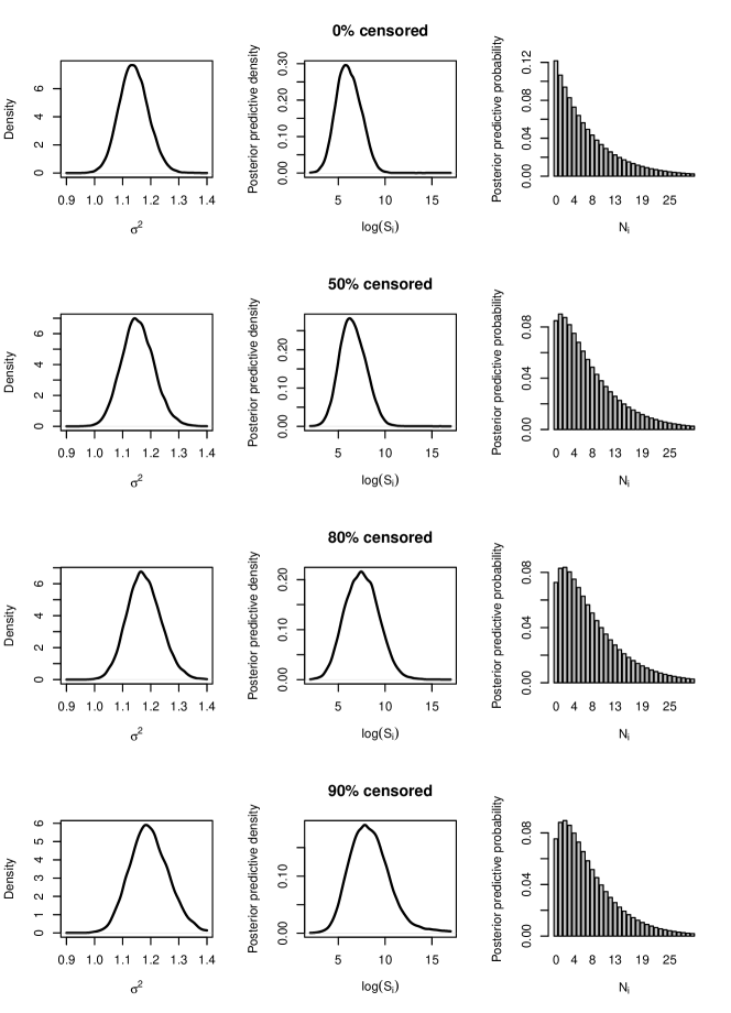
Figure 3: Posterior density for $\sigma^{2}$, and posterior predictive density for $\log(S_{i})$ and posterior predictive probability mass function for $N_{i}$ for a hypothetical new patient with covariates equal to their sample medians from our model fitted on the simulated data.

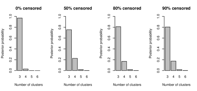
Figure 4: Posterior distribution of the number of clusters from our model fitted on the simulated data.

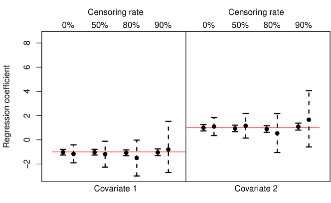
Figure 5: Posterior means (dot) and 95% marginal posterior credible intervals (lines) of the regression coefficients from our model fitted on the simulated data. The solid lines represent credible intervals for the regression coefficients $\bm{\beta}$ in (3) for the gap times model. The dashed lines correspond with the regression coefficients $\bm{\gamma}$ in (4) for the survival times. The horizontal line marks the true $\bm{\beta}=\bm{\gamma}=(-1,1)^{T}$ from which the data were simulated.

We choose hyperparameters yielding uninformative prior distributions as detailed in Section LABEL:sec:prior_spec_SM of the supplemental material. The base measure $G_{0}$ of the DP prior has high variance. A priori, $\sigma^{2}$ and $\eta^{2}$ have an expected value of one and a variance of $100$. We run the Gibbs sampler for 200 000 iterations, discarding the first 20 000 as burn-in and thinning every 10 iterations, resulting in a final posterior sample size of 18 000.

Figures 1 through 5 summarize the results. The predictions and uncertainty quantification for the number of recurrent events $N_{i}$ in Figure 1 are sensible with only 16 (5%) of the 330 credible intervals not covering the true $N_{i}$. Figures 2 and 3 show increased posterior uncertainty for higher levels of censoring. This increase in uncertainty is larger for $\delta_{i}$ , which relates to the survival time $S_{i}$, than for other parameters which relate to the recurrence process. A reason for this is that, for a censored individual $i$, often some event times are observed while $S_{i}$ is right-censored and thus not observed. The posterior mass on the actual number of clusters is marginally higher for the uncensored than for the censored data in Figure 4, although it must be noticed that posterior inference on $K$ is robust across different level of censoring. Figure 5 shows accurate inference for $\bm{\beta}$ with the uncertainty in $\bm{\gamma}$ increasing with the censoring rate as a higher censoring induces more uncertainty about the survival time $S_{i}$.

Section LABEL:sec:add_simul of the supplemental material contains additional simulation studies. Our simulations show that poster inference is robust not only to the choice of hyper-parameters of the negative binomial distribution, but also to model misspecification. Nevertheless, it must be noted that posterior mean estimates and their associated bias and mean squared errors are affected by censoring rate.

4 Application to colorectal cancer data

4.1 Data description and analysis

We apply our model to the colorectal cancer data described in Gonzalez et al.Gonzalez2005 which consider $L=403$ patients diagnosed with colorectal cancer between 1996 and 1998 in Bellvitge University Hospital in Barcelona, Spain. The data consist of hospital readmissions related to colorectal cancer surgery up until 2002 and are available as part of the R package frailtypack.(Rondeau2012, ) The date of surgery represents the origin of a patient’s recurrence process such that $T_{i0}=0$ for all $i$. Consequently, $n_{i}$ represents the number of observed gap times between subsequent hospitalizations. Patients experience between zero and 22 hospitalizations each and $\sum_{i=1}^{L}n_{i}=458$ in aggregate. Table 1 shows how they are distributed across patients. Gap times are defined as the difference between successive hospitalizations and, as such, capture both the length of stay in the hospital and the time between discharge and the next hospitalization.

Table 1: Frequency table of the number of observed gap times $n_{i}$ and, for the 109 uncensored patients, the total number of gap times $N_{i}$ in the colorectal cancer data.

$n_{i}$	0	$1$	$2$	$3$	$4$	$5$	$6$	7	$8$	$9$	$10$	$11$	$16$	$22$
Frequency (all)	199	105	45	21	15	8	4	0	1	1	1	1	1	1
Frequency (uncensored)	36	33	16	10	6	4	0	0	1	1	0	0	1	1

The main clinical outcome of interest is deterioration to death. We therefore define the survival time $S_{i}$ as the time to death. The survival times of 294 out of the 403 recurrence processes are censored due to the follow-up ending in 2022, resulting in unobserved total number of gap times $N_{i}$.

Patient characteristics considered are the binary variables 1) whether the patient received radiotherapy or chemotherapy and 2) gender, and Dukes’ tumour classification which takes as levels stage A-B, C or D. We dummy code Dukes’ classification with stage A-B as baseline resulting in a subject-specific $4$-dimensional covariate vector $\bm{x}_{i}$, with $q=4$. Table 2, and Figures 6 and 7 summarize the patient characteristics, and the gap and survival times.

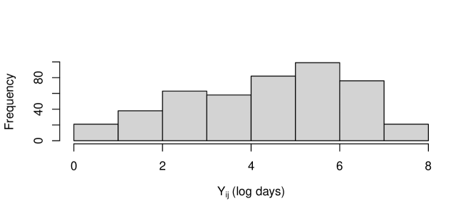
Figure 6: Histogram of the 458 observed log gap times $Y_{ij}$ in the colorectal cancer data.

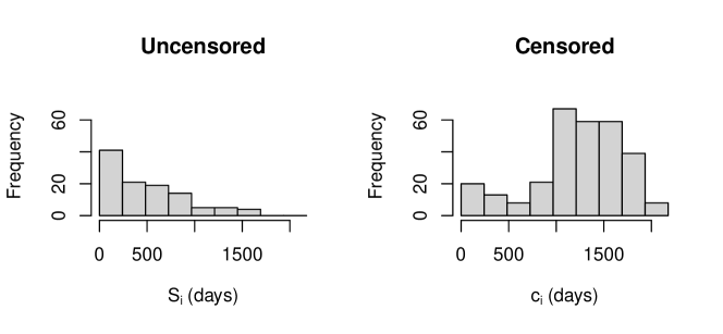
Figure 7: Histograms of the log of the 109 observed survival times $S_{i}$ (left) and the 294 censoring times (right) in the colorectal cancer data. If the survival time $S_{i}$ is observed, then $c_{i}=S_{i}$.

We use the same priors, from Section LABEL:sec:prior_spec_SM of the supplemental material, and set-up of the Gibbs sampler as the simulation study in Section 3. Then, the regression coefficients $\bm{\beta}$ and $\bm{\gamma}$ have high prior variance.

Figure 8: The posterior means (dot) of the number of gap times $N_{i}$ and 95% posterior credible intervals (lines) for each censored patient from our model fitted on the colorectal cancer data. The number of observed gap times $n_{i}$ is marked by ‘$\times$’.

4.2 Posterior inference on the number of recurrent events

Figure 8 summarizes the posterior distribution of the total number of gap times $N_{i}$ for each censored patient. The posterior means for the censored $N_{i}$ are generally in line with the observed $N_{i}$ in Table 1 though the lowest posterior mean is with 1.9 higher than the lowest observed $N_{i}$. This is expected since patients with longer survival times $S_{i}$ are both more likely to have a higher number of gap times $N_{i}$ and to be censored due to end of study. Our model flexibly captures $N_{i}$’s uncertainty, which varies notably across censored patients. These findings highlight the importance of modelling and inferring $N_{i}$ when the number of events is censored and, therefore, unknown.

4.3 Posterior inference on the regression coefficients

The regression coefficients $\bm{\beta}$ and $\bm{\gamma}$ capture the covariate effects on the recurrent event and survival processes, respectively. Figure 9 shows negative coefficients for the more advanced tumour stages C and D in the survival regression but not for the gap times model. This suggests that more severe tumours, while they negatively affect survival, do not have an effect on rehospitalization rate beyond the link between survival and hospitalization implied by our joint model.

Figure 9: Posterior means (dot) and 95% marginal posterior credible intervals (lines) of the regression coefficients from our model fitted on the colorectal cancer data. The solid lines represent credible intervals for the regression coefficients $\bm{\beta}$ in (3) for the gap times model. The dashed lines correspond with the regression coefficients $\bm{\gamma}$ in (4) for the survival times.

4.4 Posterior inference on the cluster allocation

As discussed in Section 1, the DP prior on $(\bm{m}_{i},\,\delta_{i})$ described in Section 2.3 allows for clustering of patients based on their recurrent event and survival profiles. The random effects parameters determine the clustering of patients and capture the dependence between the recurrence and survival processes. Indeed, the posterior predictive distribution of these parameters for a hypothetical new patient is multimodal as shown in Figure 10, indicating the presence of multiple patient subpopulations.

Figure 10: Contour plots of the log of the bivariate posterior predictive densities of $(m_{i1},\,\delta_{i})$ (left) and $(m_{i2},\,\delta_{i})$ (right) for a hypothetical new patient from the colorectal cancer data.

The clustering depends on both gap time trajectories and survival outcomes thanks to the joint distribution on $\bm{m}_{i}$ and $\delta_{i}$. In particular, Figure 10 reports the bivariate posterior marginals of $(m_{i1},\delta_{i})$ and $(m_{i2},\delta_{i})$, which are bimodal.

Posterior inference on the clustering structure of the patients is of clinical interest as it might guide more targeted therapies. Our Gibbs sampler provides posterior samples of the cluster allocation. Here, we report the cluster allocation that minimizes the posterior expectation of Binder’s(binder1978bayesian, ) loss function under equal misclassification costs, which is a common choice in the applied Bayesian non-parametrics literature.(lau2007bayesian, ) See Appendix B of Argiento et al.argiento2014density for computational details. Briefly, Binder’s loss function measures the difference for all possible pairs of individuals between the true probability of co-clustering and the estimated cluster allocation. In this context, the posterior estimate of the partition of the patients has three clusters, with 99% of the patients allocated to two clusters which are summarized in Table 2.

Table 2: Summary statistics of the colorectal cancer data and the posterior from our model. The two clusters are the largest from a posterior estimate of the cluster allocation that minimizes the posterior expectation of Binder’s(binder1978bayesian, ) loss function. The averages and standard deviations of posterior means are taken across patients and recurrent events. $S_{i}$ is recorded in days and $Y_{ij}$ in log days.

	Full dataset	Cluster 1	Cluster 2
Number of patients	403	292	108
Proportion censored	73%	81%	54%
Average uncensored $N_{i}$	1.78 (2.92)	0.79 (0.93)	2.68 (3.41)
Average posterior mean of $N_{i}$ (SD)	2.87 (1.95)	2.55 (1.08)	3.66 (2.91)
Average uncensored $Y_{ij}$ (SD)	4.35 (1.84)	5.55 (1.24)	3.91 (1.72)
Average posterior mean of $Y_{ij}$ (SD)	6.55 (1.39)	7.06 (0.82)	5.03 (1.52)
Average uncensored $\log(S_{i})$ (SD)	5.78 (1.03)	5.66 (1.09)	5.96 (0.93)
Average posterior mean of $\log(S_{i})$ (SD)	8.91 (2.14)	9.39 (2.03)	7.72 (1.85)
Proportion on chemotherapy	54%	55%	50%
Proportion female	41%	42%	37%
Proportion stage C	37%	34%	45%
Proportion stage D	19%	19%	17%

The largest cluster, Cluster 1, has longer gap and imputed survival times than Cluster 2. Moreover, the Kaplan-Meier curves of each cluster in Figure 11 support the conclusion that Cluster 1 includes patients with longer survival times than Cluster 2.

Figure 11: Kaplan-Meier survival estimates for the two largest clusters estimated by minimizing the expectation of Binder’s(binder1978bayesian, ) loss function under the posterior from our model on the colorectal cancer data. The solid and dashed lines represent Cluster 1 and 2, respectively. The curves are based on the posterior means of $\log(S_{i})$.

As shown in Table 2, Cluster 1 has a higher censoring rate than Cluster 2, as one might expect at longer survival times. The lower prevalence of late stage tumours in Cluster 1 also confirms that it includes healthier subjects than Cluster 2.

Figures LABEL:fig:readmission_variance and LABEL:fig:readmission_K in the supplemental material contain additional posterior results. Section LABEL:sec:AF of the supplemental material presents an application to atrial fibrillation data.

5 Comparison with other models

5.1 Cox proportional hazards model

We now compare our results on the colorectal cancer data to those obtained from the Cox proportional hazards model which is one of the most popular semi-parametric models in survival analysis with covariates. In this model, the hazard function for mortality is ${h_{i}(t\mid\bm{\theta})}=h_{0}(t)\,\exp({\bm{z}_{i}^{T}\bm{\theta}})$ where $h_{0}(t)$ is the baseline hazard function, $\bm{z}_{i}$ is a vector of covariates and $\bm{\theta}$ is a vector of regression coefficients. Here, a larger value of $\bm{z}_{i}^{T}\bm{\theta}$ leads to shorter survival times. This contrasts with (4) from our model where a larger $\bm{x}_{i}^{T}\bm{\gamma}$ is associated with longer survival times.

Our model allows for dependence between the gap and survival times. Therefore, for a fairer comparison when fitting the Cox proportional hazard model, we include a patient’s log mean gap time in the covariate vector $\bm{z}_{i}$ in addition to the four covariates included in $\bm{x}_{i}$ described in Section 4.1. As a result, the 199 individuals with no observed gap times are excluded. Table LABEL:tab:readmission_PH in the supplemental material shows the covariate effects on survival from the Cox proportional hazards model. The statistically significant effects agree with those from our model in Figure 9.

5.2 Joint frailty model

We also compare our model with the joint frailty model by Rondeau et al.Rondeau2007 as implemented in the R package frailtypack.(Rondeau2012, ) The model estimates the hazard functions of rehospitalization and mortality jointly using two patient-specific frailty terms, namely $u_{i}$ and $v_{i}$. The frailty term $u_{i}$ captures the association between rehospitalization and mortality while $v_{i}$ appears solely in the rehospitalization rate. Specifically, the hazard functions are $r_{i}(t\mid u_{i},v_{i},\bm{\beta})=u_{i}\,v_{i}\,r_{0}(t)\,\exp({\bm{x}_{i}^{T}\bm{\beta}})$ for rehospitalization and $\lambda_{i}(t|u_{i},\bm{\gamma})=u_{i}\,\lambda_{0}(t)\,\exp({\bm{x}_{i}^{T}\bm{\gamma}})$ for mortality. Here, $r_{0}(t)$ and $\lambda_{0}(t)$ are baseline hazard functions, and $\bm{x}_{i}$, $\bm{\beta}$ and $\bm{\gamma}$ are defined as in Section 2. The random effects distributions are specified as follows: $v_{i}\sim\text{Gamma}(1/\rho,\,1/\rho)$ and $u_{i}\sim\text{Gamma}(1/\epsilon,\,1/\epsilon)$ independently for $i=1,\dots,L$.

The comparison of the joint frailty model results in Table LABEL:tab:readmission_frailty of the supplemental material with our results in Figure 9 shows that both models find that late stage tumours are associated with shorter survival. For the other covariates, the comparison is inconclusive with the joint frailty model finding statistically significant effects where our model does not and vice versa.

Finally, the estimate of $\rho$ is $0.007$ with a standard error of $0.001$. This suggests heterogeneity between patients that is not explained by the covariates. The estimate of $\epsilon$ is $0.073$ with a standard error of $0.13$. This implies that the rate of rehospitalizations is positively associated with mortality. These results are in line with the posterior clustering results from our model in Table 2 where Cluster 1 is characterized by both the longest gap times and the longest survival times.

5.3 Bayesian semi-parametric model from Paulon et al.Paulon2018

For a more direct comparison, we consider the method proposed by Paulon et al.Paulon2018 as it models the gap and survival times jointly using Bayesian non-parametric priors. Paulon et al.Paulon2018 assume that, conditionally on all parameters and random effects, the gap times are independent of both each other and the survival time. This contrasts with the temporal dependence between gap times in (3). Shared random effects induce dependence between different gap times of the same patient. Specifically, Paulon et al.Paulon2018 assume $Y_{ij}\sim\mathcal{N}({\bm{x}}_{i}^{T}{\bm{\beta}}+\alpha_{i},\,\sigma_{i}^{2})$ independently for $j=1,\dots,n_{i}+1$ and $i=1,\dots,L$, and

$$\log(S_{i})\sim\mathcal{N}({\bm{x}}_{i}^{T}{\bm{\gamma}}+\psi\,\alpha_{i},\,\eta^{2}),$$ (5)

independently for $i=1,\dots,L$, where $\bm{x}_{i}$, $\bm{\beta}$ and $\bm{\gamma}$ are defined as in Section 2, and $\alpha_{i}$ and $\sigma_{i}$ are random effects. Paulon et al.Paulon2018 do not model the total number of gap times $N_{i}$ but assume that each patient has a censored $(n_{i}+1)$th log gap time $Y_{i(n_{i}+1)}$. They also assume a priori independence among $\bm{\beta}$, $\bm{\gamma}$, $\psi$, $\eta$ and $(\bm{\alpha},\,\bm{\sigma}^{2})$. The random effects $(\alpha_{i},\,\sigma_{i}^{2})\sim G$ independently for $i=1\dots,L$ where $G\sim\text{DP}(M,\,G_{0})$ with $M\sim\text{Uniform}(a_{M},\,b_{M})$ and $G_{0}=\mathcal{N}(0,\,\alpha_{0}^{2})\times\text{Inv-Gamma}(a_{\sigma},\,b_{\sigma})$. The priors on $\bm{\beta}$, $\bm{\gamma}$ and $\eta^{2}$ are set as in Section 2.3. Finally, ${\psi}\sim\mathcal{N}(0,\,\psi_{0}^{2})$.

In fitting this model to the colorectal cancer data, we specify the same $\bm{x}_{i}$ and the same hyperparameters for the priors on $\bm{\beta}$, $\bm{\gamma}$ and $\eta^{2}$ as in Section 4.1. Furthermore, we set $a_{M}=0.3$, $b_{M}=5$, $\alpha_{0}^{2}=100$, $a_{\sigma}=2.01$, $b_{\sigma}=1.01$ and $\psi_{0}^{2}=100$. This model yields conclusions that are largely consistent with those from our model. In particular, the posterior distributions on the coefficients in Figure LABEL:fig:readmission_CI_paulon of the supplemental material mimic our results in Figure 9 except for the effect of tumour stage on recurrence. Also, the posterior on $\psi$ in (5) concentrates between 1.3 and 1.7 per Figure LABEL:fig:readmission_psi of the supplemental material. This parameter captures the strength of the relationship between gap and survival times. Thus, the time between hospitalizations and survival have a positive association. This is consistent with the clustering results obtained from our model in Table 2. Lastly, the posterior on the number of clusters for this model and our model vary slightly, with a mode of three clusters for our model in Figure LABEL:fig:readmission_K of the supplemental material while Figure LABEL:fig:readmission_K_paulon of the supplemental material has the mode at five for the model from Paulon et al.Paulon2018 This is not surprising as our model introduces more structure: a temporal model for the gap time, as well as process-specific frailty terms which are jointly modelled non-parametrically. Moreover, the number of recurrent events is a random quantity and object of inference, which also informs the dependence between the two processes, in addition to the truncation $T_{iN_{i}}\leq S_{i}$ of (3). In contrast, Paulon et al.Paulon2018 can capture such dependence using only $\psi$ in (5), and the gap times are conditionally independent given $\psi$ and the remaining parameters, with the total number of gap times per individual assumed arbitrarily large.

6 Discussion

We introduce a joint model on recurrence and survival that explicitly treats the number of recurrent events $N_{i}$ before the terminal event as a random variable and object of inference as $N_{i}$ is often of interest in applications. Additionally, the explicit modelling of $N_{i}$ as well as the specification of a joint distribution for the random effects of the recurrence and survival processes induces dependence between these processes. Moreover, temporal dependence among recurrent events is introduced through a first-order autoregressive process on the gap times. Extension to a more complex temporal structure is in principle straightforward. The model allows for estimating covariates effects on the recurrence and survival processes by introducing appropriate regression terms. Our model can readily accommodate a different prior on the number of recurrent events than the negative binomial distribution. For instance, an earlier version of this workvandenBoom2020 used a Poisson distribution. The use of a non-parametric prior as random effects distribution allows for extra flexibility, patient heterogeneity and data-driven clustering of the patients.

We use log-normal kernels for the non-parametric survival and gap time distributions. Use of different kernels is computationally impracticable as then the evaluation of the normalization constant of ${p(\bm{Y}_{i},S_{i}\mid\text{\textemdash})}$ becomes considerably more expensive. This evaluation is already the computational bottleneck of our method as it happens frequently as part of slice sampling at each iteration of the Gibbs sampler. The reasons why using different kernels is problematic are twofold: Firstly, the log-normal kernel for the gap times enables the Fenton-Wilkinson(Fenton1960, ) approximation for the distribution of $T_{iN_{i}}$. Other kernels for the gap times might not enable such computationally efficient evaluations. For instance, Proposition 1 of El Bouanani and Ben-AzzaElBouanani2015 gives rise to an approximation when using a Weibull kernel which is computationally more involved than the Fenton-Wilkinson method. Secondly, the current combination of the Fenton-Wilkinson method and a log-normal survival kernel reduce the normalization constant of ${p(\bm{Y}_{i},S_{i}\mid\text{\textemdash})}$ to a tail probability of a univariate Gaussian as detailed in Section LABEL:sec:constant of the supplemental material. A different survival kernel, say a Weibull kernel, would require computation which is an order of magnitude more expensive, such as numerical integration to evaluate the normalization constant, or further approximation.

The simulation study shows the effectiveness of posterior inference on the number of recurrent events $N_{i}$. Comparison with the Cox proportional hazards model, the joint frailty model(Rondeau2007, ) and the Bayesian semi-parametric model from Paulon et al.Paulon2018 yields consistent results, with few exceptions in the estimation of covariate effects. This discrepancy might be the result of the fact that these models have fewer parameters and assume a single patient population while our model detects multiple subpopulations. Moreover, in our model specification a further level of dependence is introduced through the distribution of the number of gap times. More flexibility, if required by the application, could be achieved by including also the hyper-parameters of the distribution of the number of gap-times in the nonparametric component of the model.

This research is partially supported by the Singapore Ministry of Health’s National Medical Research Council under its Open Fund - Young Individual Research Grant (OFYIRG19nov-0010).

The Authors declare that there is no conflict of interest.

The supplemental material referenced in the text is available online. The code that generated the results in this paper is available at https://github.com/willemvandenboom/condi-recur.

See pages - of supp_web.pdf

References

- (1) Jencks SF, Williams MV and Coleman EA. Rehospitalizations among patients in the medicare fee-for-service program. New England Journal of Medicine 2009; 360(14): 1418–1428. 10.1056/nejmsa0803563.
- (2) McIlvennan CK, Eapen ZJ and Allen LA. Hospital readmissions reduction program. Circulation 2015; 131(20): 1796–1803. 10.1161/circulationaha.114.010270.
- (3) Zuckerman RB, Sheingold SH, Orav EJ et al. Readmissions, observation, and the hospital readmissions reduction program. New England Journal of Medicine 2016; 374(16): 1543–1551. 10.1056/nejmsa1513024.
- (4) Cook RJ and Lawless JF. The statistical analysis of recurrent events. Springer, New York, 2007. 10.1007/978-0-387-69810-6.
- (5) Liu L, Wolfe RA and Huang X. Shared frailty models for recurrent events and a terminal event. Biometrics 2004; 60(3): 747–756. 10.1111/j.0006-341x.2004.00225.x.
- (6) Rondeau V, Mathoulin-Pelissier S, Jacqmin-Gadda H et al. Joint frailty models for recurring events and death using maximum penalized likelihood estimation: Application on cancer events. Biostatistics 2007; 8(4): 708–721. 10.1093/biostatistics/kxl043.
- (7) Ye Y, Kalbfleisch JD and Schaubel DE. Semiparametric analysis of correlated recurrent and terminal events. Biometrics 2007; 63(1): 78–87. 10.1111/j.1541-0420.2006.00677.x.
- (8) Huang CY, Qin J and Wang MC. Semiparametric analysis for recurrent event data with time-dependent covariates and informative censoring. Biometrics 2010; 66(1): 39–49. 10.1111/j.1541-0420.2009.01266.x.
- (9) Sinha D, Maiti T, Ibrahim JG et al. Current methods for recurrent events data with dependent termination. Journal of the American Statistical Association 2008; 103(482): 866–878. 10.1198/016214508000000201.
- (10) Ouyang B, Sinha D, Slate EH et al. Bayesian analysis of recurrent event with dependent termination: An application to a heart transplant study. Statistics in Medicine 2013; 32(15): 2629–2642. 10.1002/sim.5717.
- (11) Olesen AV and Parner ET. Correcting for selection using frailty models. Statistics in Medicine 2006; 25(10): 1672–1684. 10.1002/sim.2298.
- (12) Huang X and Liu L. A joint frailty model for survival and gap times between recurrent events. Biometrics 2007; 63(2): 389–397. 10.1111/j.1541-0420.2006.00719.x.
- (13) Yu Z and Liu L. A joint model of recurrent events and a terminal event with a nonparametric covariate function. Statistics in Medicine 2011; 30(22): 2683–2695. 10.1002/sim.4297.
- (14) Bao Y, Dai H, Wang T et al. A joint modelling approach for clustered recurrent events and death events. Journal of Applied Statistics 2012; 40(1): 123–140. 10.1080/02664763.2012.735225.
- (15) Liu L, Huang X, Yaroshinsky A et al. Joint frailty models for zero-inflated recurrent events in the presence of a terminal event. Biometrics 2015; 72(1): 204–214. 10.1111/biom.12376.
- (16) Yu Z, Liu L, Bravata DM et al. Joint model of recurrent events and a terminal event with time-varying coefficients. Biometrical Journal 2013; 56(2): 183–197. 10.1002/bimj.201200160.
- (17) Li Z, Chinchilli VM and Wang M. A Bayesian joint model of recurrent events and a terminal event. Biometrical Journal 2019; 61(1): 187–202. 10.1002/bimj.201700326.
- (18) Li Z, Chinchilli VM and Wang M. A time-varying Bayesian joint hierarchical copula model for analysing recurrent events and a terminal event: an application to the cardiovascular health study. Journal of the Royal Statistical Society: Series C (Applied Statistics) 2019; 69(1): 151–166. 10.1111/rssc.12382.
- (19) Paulon G, De Iorio M, Guglielmi A et al. Joint modeling of recurrent events and survival: A Bayesian non-parametric approach. Biostatistics 2018; 10.1093/biostatistics/kxy026. Kxy026.
- (20) Tallarita M, De Iorio M, Guglielmi A et al. Bayesian autoregressive frailty models for inference in recurrent events. The International Journal of Biostatistics 2020; 16(1): 1–18. 10.1515/ijb-2018-0088.
- (21) Kansagara D, Englander H, Salanitro A et al. Risk prediction models for hospital readmission: A systematic review. JAMA 2011; 306(15): 1688. 10.1001/jama.2011.1515.
- (22) Futoma J, Morris J and Lucas J. A comparison of models for predicting early hospital readmissions. Journal of Biomedical Informatics 2015; 56: 229–238. 10.1016/j.jbi.2015.05.016.
- (23) Mahmoudi E, Kamdar N, Kim N et al. Use of electronic medical records in development and validation of risk prediction models of hospital readmission: systematic review. BMJ 2020; 369: m958. 10.1136/bmj.m958.
- (24) Green PJ. Reversible jump Markov chain Monte Carlo computation and Bayesian model determination. Biometrika 1995; 82(4): 711–732. 10.1093/biomet/82.4.711.
- (25) Neal RM. Slice sampling. The Annals of Statistics 2003; 31(3): 705–767. 10.1214/aos/1056562461.
- (26) Ferguson TS. A Bayesian analysis of some nonparametric problems. The Annals of Statistics 1973; 1(2): 209–230.
- (27) Sethuraman J. A constructive definition of Dirichlet priors. Statistica Sinica 1994; 4(2): 639–650.
- (28) Aalen OO and Husebye E. Statistical analysis of repeated events forming renewal processes. Statistics in Medicine 1991; 10(8): 1227–1240. 10.1002/sim.4780100806.
- (29) Lo AY. On a class of Bayesian nonparametric estimates: I. density estimates. The Annals of Statistics 1984; 12(1). 10.1214/aos/1176346412.
- (30) De Iorio M, Johnson WO, Müller P et al. Bayesian nonparametric nonproportional hazards survival modeling. Biometrics 2009; 65(3): 762–771. 10.1111/j.1541-0420.2008.01166.x.
- (31) Fenton L. The sum of log-normal probability distributions in scatter transmission systems. IEEE Transactions on Communications 1960; 8(1): 57–67. 10.1109/tcom.1960.1097606.
- (32) Neal RM. Markov chain sampling methods for Dirichlet process mixture models. Journal of Computational and Graphical Statistics 2000; 9(2): 249–265. 10.1080/10618600.2000.10474879.
- (33) González JR, Fernandez E, Moreno V et al. Sex differences in hospital readmission among colorectal cancer patients. Journal of Epidemiology & Community Health 2005; 59(6): 506–511. 10.1136/jech.2004.028902.
- (34) Rondeau V, Mazroui Y and Gonzalez JR. frailtypack: An R package for the analysis of correlated survival data with frailty models using penalized likelihood estimation or parametrical estimation. Journal of Statistical Software 2012; 47(4): 1–28. 10.18637/jss.v047.i04.
- (35) Binder DA. Bayesian cluster analysis. Biometrika 1978; 65(1): 31–38.
- (36) Lau JW and Green PJ. Bayesian model-based clustering procedures. Journal of Computational and Graphical Statistics 2007; 16(3): 526–558.
- (37) Argiento R, Cremaschi A and Guglielmi A. A “density-based” algorithm for cluster analysis using species sampling Gaussian mixture models. Journal of Computational and Graphical Statistics 2014; 23(4): 1126–1142.
- (38) van den Boom W, Tallarita M and De Iorio M. Bayesian joint modelling of recurrence and survival: a conditional approach, 2020. arXiv:2005.06819v1.
- (39) Bouanani FE and Ben-Azza H. Efficient performance evaluation for EGC, MRC and SC receivers over Weibull multipath fading channel. In Lecture Notes of the Institute for Computer Sciences, Social Informatics and Telecommunications Engineering. Springer International Publishing, 2015. pp. 346–357. 10.1007/978-3-319-24540-9_28.