A protocol of potential advantage in the low frequency range to
gravitational wave detection with space based optical atomic clocks

Abstract

A recent proposal describes space based gravitational wave (GW) detection with optical lattice atomic clocks [Kolkowitz et. al., Phys. Rev. D 94, 124043 (2016)] kpy16 . Based on their setup, we propose a new measurement method for gravitational wave detection in low frequency with optical lattice atomic clocks. In our method, n successive Doppler signals are collected and the summation for all these signals is made to improve the sensitivity of the low-frequency GW detection. In particular, the improvement is adjustable by the number of Doppler signals, which is equivalent to that the length between two atomic clocks is increased. Thus, the same sensitivity can be reached but with shorter distance, even though the acceleration noises lead to failing to achieve the anticipated improvement below the inflection point of frequency which is determined by the quantum projection noise. Our result is timely for the ongoing development of space-born observatories aimed at studying physical and astrophysical effects associated with low-frequency GW.

I Introduction

Direct detection of gravitational wave (GW) carries important implications both for astronomy where information about astrophysical sources can be obtained and for fundamental physics where aspects of relativistic theories of gravity can be tested kst87 . In 2016, the first detection of GW from two merging black holes bpa16 was reported by the advanced Laser Interferometer Gravitational-wave Observatory (aLIGO), the famous terrestrial laser interferometer observatory. A number of analogous GW events were detected bpa162 ; bpa17 ; bpa172 ; bpa173 subsequently, all lying in the frequency range of above dozens of Hertz (Hz). In the lower frequency range, where prospective GW sources might stem from cosmological origin, such as the very early phase of the Big Bang, or the more speculative astrophysical objects like cosmic strings or domain boundaries aas12 ; aab12 , GW remains elusive due to insufficient sensitivities. In fact, methods such as laser interferometry in space lisa96 ; pas12 ; pas17 ; luo16 ; hw17 , pulsar timing arrays dcb86 ; jcs10 , and Doppler tracking system jwa06 etc., have been considered for detecting low frequency GW. Laser interferometers with very long arm lengths can also be used to detect low-frequency GW, although this remains as challenging. One of the earliest and still popular proposals in this direction belongs to the Laser Interferometer Space Antenna (LISA), whose planned launch date is arranged in about 2034 lisa . In view of the successful observations of GW, it is important and timely to study other related methods for the detection of low-frequency GW.

In this study, we investigate and extend the method of spacecraft Doppler tracking. This precise technique traces back to the GP-A suborbital experiments that measured the general relativistic redshift in the earth’s static gravitational fields rvc80 , although the facilitating idea that fractional frequency fluctuation caused by GW on one-way Doppler of an earth-based GW detector was studied already in 1970 wjf70 , and soon afterwards, followed with a survey for its prospects of GW detection, by Davis in two-way Doppler with deep space probes rwd74 . The traditional technique for tracking distant spacecraft is to precisely monitor the Doppler shift of a sinusoidal electromagnetic signal, which is continuously transmitted to the spacecraft and coherently re-transmitted back to earth jcb83 . In the Doppler tracking technique, the Earth and an interplanetary spacecraft act as free test masses. The Doppler tracking system continuously measures their relative dimensionless velocity, $\Delta\upsilon/c=\Delta\nu/\nu_{0}$, where $\Delta\upsilon$ is the relative velocity, $\Delta\nu$ is the associated Doppler frequency change, and $\nu_{0}$ is the carrier frequency of the microwave link. A gravitational wave of strain amplitude $h\left(t\right)$ propagating through the radio link causes small perturbations in the Doppler time series of $\Delta\nu\left(t\right)/\nu_{0}$ jwa06 ; ewr75 . Recently, Kolkowitz et al kpy16 proposes a space-based gravitational wave detector consisting of two spatially separated, drag-free satellites sharing ultrastable optical laser light over a single baseline and augmented by dynamical decoupling bzy13 for improved sensitivity. In their method, atomic clocks (instead of atomic interferometers) serve as GW sensors phk13 ; jmh16 ; cwy15 , and the cumulative large-momentum-transfer experienced in atomic interferometry is introduced into a system of clocks to enhance detection sensitivity nct17 . A Doppler tracking system for GW detection via Double Optical Clock in Space (DOCS) is also proposed sww18 , in which the frequency range covers $10^{-4}$ Hz to $10^{-2}$ Hz with an overall estimated sensitivity of $5\times 10^{-19}$.

Although the last two proposals mentioned above can be sensitive to the low GW frequency around $10^{-3}$ Hz, they need the arm length (distance between two satellites) to be 1AU, which requires high optical power due to optical diffraction. And for the same reason, the signal recycling cavity used in LIGO is impossible for long baseline space-based optical interferometers. We find that we can use the similar scheme to Ref. kpy16 but performed with the recycling laser pulses in space to increase equivalently the arm length of shorter space-based interferometer. It is helpful for some plans like TianQin or Taiji Program in Space, in both of which the length of laser path is about ${\sim}10^{8}$ m luo16 ; hw17 . This paper is structured as follows. First, we introduce the method of Doppler tracking for GW detection, while the one-way clock interferometry is introduced in detail in second section. In third section, we investigate the theory about sensitivity curves and compare the one-way method with the two-way or two one-way methods schematically, from which one can see the longer Ramsey precession time can increase the sensitivity of the optical atomic clock detector. In fourth section, we propose the recycling method which is equivalently to increase the effective arm length, and discuss its limits. Finally, we conclude in the fifth section.

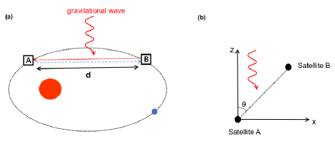
Figure 1: (Color online) (a) The configuration for the proposed GW detector of Ref. kpy16 , which consists of two identical drag-free satellites, A and B, in a heliocentric orbit, separated from each other by a distance $d$. Each satellite maintains a free-floating reference mass, an ultrastable laser, and a strontium optical lattice clock. The measurement scheme we propose differs from that of Ref. kpy16 , and will be discussed in Sect. III. (b) Illustration of the geometric configuration.

II Doppler Tracking Signal

The scheme for Doppler tracking is shown in Fig. 1(a), which is the same as found in Ref. kpy16 , except that we will implement a different operation protocol to be discussed in the fourth section. The two drag-free satellites A and B are launched into a heliocentric orbit, each equipped with an optical clock. The distance $d$ between the two satellites is set to $5\times 10^{10}$ m. Via two synchronized clocks and radio instruments on board, a radio signal can be transmitted from A (B) to B (A), and the Doppler signals as functions of time can be collected simultaneously on the two satellites, i.e., two or bidirectional Doppler tracking measurements are carried out simultaneously.

Figure 1(b) illustrates the simple geometric configuration for the discussed Doppler tracking system for GW detection, where satellite A is set at the origin and the two satellites lie in the $x$-$z$ plane separated by a distance $d$. Assuming that the GW is propagating along the $z$-axis direction through the Doppler tracking system and the corresponding spacetime can be described by the perturbed metric

$$ds^{2}=-c^{2}dt^{2}+\left(1+h\right)dx^{2}+\left(1-h\right)dy^{2}+dz^{2},$$ (1)

where $h=h\left(t-z\right)$ is exceedingly small compared with unity and it describes the strain field of a train of plane gravitational waves. The spacetime Eq. (1) has symmetries generated by the Killing vectors: {$\frac{\partial}{\partial x},\frac{\partial}{\partial y},\frac{\partial}{\partial z}+\frac{\partial}{\partial t}$}.

The influence of GW on the signal of a Doppler tracking system is easily calculated. For a light signal sent at time $t$ from system $A$ to system $B$, the light at $A$ can be described by a null vector with the form

$$\sigma_{0}=\left(-\nu_{0}\right)\left[dt+\left(1+h_{0}/{2}\right)\sin\theta dx+\cos\theta dz\right],$$ (2)

with $\theta$ the angle between the link line $AB$ and $z$-axis. $\nu_{0}$ is the observed frequency of the light, and $h_{0}$ is the value of $h\left(t-z\right)$ at the emitter $A$. When the light arrives at the receiver $B$, its frequency and the GW strain becomes $\nu_{1}$ and $h_{1}$. Define the frequency shift parameter

$$z\equiv\frac{\nu_{1}-\nu_{0}}{\nu_{0}},$$ (3)

for the situation considered here, it is given by ewr75 ,

$$z_{AB}=\frac{1}{2}\left(1+\cos\theta\right)\left(h_{0}-h_{1}\right),$$ (4)

with $h_{1}=h\left[t+\left(1-\cos\theta\right){d}/{c}\right]$ according to the coordinates used in Fig. 1(b) where point $B$ is specified by $x={d\sin\theta}$, $y=0$, and $z={d\cos\theta}$. The result given in Eq. (4) is identical to that obtained from calculating directly the change of the distance between $A$ and $B$ kpy16 . If $\theta=0$, the light photons are sent out parallel to the GW normal, $z_{AB}=0$; If $\theta={\pi}/{2}$, the photons intersect perpendicularly the direction of GW propagation, $z_{AB}=\left[h\left(t\right)-h\left(t+{d}/{c}\right)\right]/2$. For simplicity, in what follows we take the latter case of $\theta={\pi}/{2}$ to calculate the maximal GW signal. When a particular Fourier component of the GW $h\left(t\right)=\left|h\right|\sin\left(2\pi ft+\varphi\right)$ with an amplitude $\left|h\right|$ and an arbitrary phase $\varphi$ is considered, the signal becomes $z={\Delta\nu}/{\nu}=-\left|h\right|\cos\left[2\pi f\left(t+{d}/{(2c)}\right)+\varphi\right]\sin(\pi f{d}/{c})$ for perpendicular light propagation, which results in the maximal fractional frequency difference between the two clocks occurring at $f=c/2d$.

At frequencies other than the optimal, the magnitude of the detectable GW signal is modulated by the inherent sensitivity of the specific setup, as captured by the detector’s transfer function $\Gamma\left(f\right)$ and the degree of system’s susceptibility to noise crl03 . For the one-way Doppler shift, Eq. (4) can be expressed in Fourier space as

$$Z_{AB}\left(f\right)=\frac{1}{2}H\left(f\right)\left(1-e^{i2\pi fd/c}\right)$$ (5)

where capital lettered functions denote Fourier transforms $Z\left(f\right)=\int dte^{i2\pi ft}z\left(t\right)$ and $H\left(f\right)=\int dte^{i2\pi ft}h\left(t\right)$. The modulation factor to $H(f)$, $\Gamma_{\nu}\left(f\right)=\left|\left(1-e^{i2\pi fd/c}\right)/2\right|^{2}=\sin^{2}\left(\pi fd/c\right)$, depends only on the geometry of the detector and is called geometric transfer function, which differs from its counterpart $\Gamma_{\phi}\left(f\right)=\sin$c${}^{2}\left(\pi fd/c\right)$ for phase detectors rs97 .

The actual measured GW signal for the clock-based detector also depends on the measurement scheme used for the atoms. A long integration time $T$ increases the sensitivity, but is limited by atomic linewidth, $T_{\max}=1/(2\pi\Delta_{A})\approx 160$ s, where the transition linewidth is $\Delta_{A}=1$ mHz lby15 ; bzl06 . The signal acquired for a clock measurement between $t_{0}$ and $t_{0}+T$ is therefore given by

$$\bar{z}=\frac{1}{T}\left|\int_{t_{0}}^{T+t_{0}}z\left(t\right)dt\right|=\left|\int_{-\infty}^{\infty}dtF\left(t_{0}-t\right)z\left(t\right)\right|,$$ (6)

where $F\left(t\right)$ describes a window function that captures the measurement sequence of duration $T$ for a specific protocol. With the Ramsey sequence ($\pi/2$ pulse at the beginning and another $\pi/2$ pulse at the end and ignoring the finite pulse operation durations), the window function reduces to $F\left(t\right)=1/T$ for $t\in\left[-T,0\right]$ and $F\left(t\right)=0$ otherwise. For a continuous GW with $h\left(t\right)=\left|h\right|\sin\left(2\pi ft+\varphi\right)$, this gives the one-way result as

$$\bar{z}_{AB} =\frac{\left|h\right|}{\pi fT}\left|\sin\left(\pi f{d}/{c}\right)\sin\left(\pi fT\right)\right.$$

$$\left.\times\cos\left[\pi f\left(2t_{0}+{d}/{c}+T\right)+\varphi\right]\right|,$$ (7)

The signal considered above is continuous. It can be made simpler by adapting the starting time of the measurement to account for $\varphi$ and thus set the argument of the cosine to $0$ to give the maximum

$$\bar{z}_{AB}=\left|h\right|\left|\sin\left(\pi f{d}/{c}\right)\mathrm{sinc}\left(\pi fT\right)\right|.$$ (8)

III Sensitivity Curve

In the initial Doppler tracking scheme jwa06 , a two-way, or two one-way-trip measurement method is used. A recent different proposal called DOCS sww18 , on the other hand, makes use of the differential signal from the two one-way-trip measurements. They are briefly summarized below and compared to each other based on the protocol put forward in Ref. kpy16 , in search for any possible improvement for GW detection.

The two-way method involves light being reflected or re-emitted from $B$ along the reverse trajectory (for the first trip of $A$ to $B$), and detected in the end at the original place $A$ (at $t={2d}/{c}$). The reversed return trip for the light is expressed as

$$\sigma_{0}^{{}^{\prime}}=\left(-\nu_{1}\right)\left(dt-\left(1+h_{1}/{2}\right)\sin\theta dx-\cos\theta dz\right).$$ (9)

When light returns to ${A}$, its frequency and strain are changed into $\nu_{2}$ and $h_{2}=h\left(t+{2d}/{c}\right)$ respectively. Thus, an observer at ${A}$ can calculate the Doppler shift of the returning light ewr75 according to

$$z_{ABA}=z_{AB}+z_{BA} =\left(h_{0}-h_{1}\right)\left(1+\cos\theta\right)/{2}$$

$$+\left(h_{1}-h_{2}\right)\left(1-\cos\theta\right)/{2}.\ \ \ \ \ \$$ (10)

As in the case of the one-way method above, one can obtain the corresponding two-way result as

$$\bar{z}_{ABA}=\left|h\right|\left|\sin\left(2\pi f{d}/{c}\right)\mathrm{sinc}\left(\pi fT\right)\right|.$$ (11)

where it is noticed that when the frequency $f=m/T$ ($m$ is the integer) and distance $d=cT/2$, some zero points are taken, which will lead to the divergence for the calculation of sensitivity below. However, the infinity is not seen in all figures about the sensitivity curves because data point acquisition is not dense enough in our numerical calculation.

Usually, one expects the signal to noise can be improved by the constraint of the common noise modes when the signals of the two separate satellites are compared, as discussed before mt96 ; prv86 ; lhh00 ; tzz15 . Based on the scheme of Fig. 1, an improved low-frequency result might be obtained from the difference of the two one-way signals, as was studied recently in Ref. sww18 and given by

$$\bar{z}_{ABD}=\left|h\right|\left|\left(1-\cos\left(2\pi f{d}/{c}\right)\right)\mathrm{sinc}\left(\pi fT\right)\right|.$$ (12)

where the average is made according to Eq. (6) with $z\left(t\right)$ replaced by the formula $z_{ABD}=z_{AB}-z_{BA}$. Although experimental conditions like noises might be different for the two way and two one-way implementation, it is concerned here that how the two data combinations resist the quantum projection noise respectively through the discussion about the sensitivity below.

In order to estimate the sensitivity, one analyzes the limit imposed by the noise (as signal strength). Following the steps of Ref. kpy16 , the smallest detectable fractional frequency difference for total measurement time $\tau=1$ s constrained by noise is given by

$$\sigma_{\min}\left(\tau\right)=\frac{\delta\nu_{\min}}{\nu}=\frac{\sqrt{\Delta_{A}}}{\nu\sqrt{2\pi\tau N}}\simeq 1.1\times 10^{-20}/\sqrt{\mathrm{Hz}}\,,$$ (13)

where the frequency of the optical clock transition is $\nu=430$ THz lby15 ; bzl06 , the transition linewidth is $\Delta_{A}=1$ mHz and the atomic number is $N=7\times 10^{6}$. Thus, the smallest measurable GW-induced strain can be determined by $\bar{z}=\sigma_{\min}\left(\tau\right)$, but the sensitivity curve is made using the general noise expression, $\sigma^{2}\left(\tau\right)=\frac{1}{\left(2\pi\upsilon\right)^{2}T\tau}\left(\frac{1}{N}+\frac{T}{\tau}\sqrt{\frac{h\upsilon\Delta_{L}}{\eta P}}\right)$ where $\Delta_{L}$ is the linewidth of the laser, $P$ is the power of the laser, and $\eta$ is the detector quantum efficiency, which is presented in Fig. 2. It shows that two-way method can shift the optimal measurement to a lower frequency, which can be extended to the general case discussed in the next section.

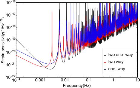
Figure 2: (Color online) Comparing the sensitivity curves for one-way, two-way, and two one-way measurement protocols.

IV Recycling scheme

The protocol we suggest consists of $n$ successive one-way-trip, or $n$-way light propagation back and forth: the first laser light is sent at time $t$ from $A$ to $B$. The moment $B$ receives the light from $A$, it re-transmits a laser to $A$. Such a sequence between $A$ and $B$ is alternately repeated with every trip of the light path experiences the change due to GW. Noticed that in the scheme described in Fig. 1, the distance between two atomic clocks just matches the measurement time determined by atomic linewidth, that is $T_{\max}=1/(2\pi\Delta_{A})=160$ s. So here the shorter distance has to be considered for the implementation of $n$-way method. For example, if the distance $d=5\times 10^{8}$ m is considered, $n$ will be constrained.

The signal for the $i$th one-way-trip is

$$z_{i}=\frac{\nu_{i}-\nu_{i-1}}{\nu_{i-1}}=\frac{1}{2}\left(1+\left(-1\right)^{i-1}\cos\theta\right)\left(h_{i-1}-h_{i}\right),$$ (14)

where

$$h_{i}=h\left(t+\sum_{m=1}^{i}\left(1+\left(-1\right)^{m}\cos\theta\right){d}/{c}\right).$$ (15)

Summing up to get the total signal, we find

$$Z_{T} =\frac{\nu_{n}-\nu_{0}}{\nu_{0}}=\sum_{m=1}^{n}z_{m}\left(t\right)$$

$$=\frac{1}{2}\left(1+\cos\theta\right)h_{0}-\frac{1}{2}\left(1+\left(-1\right)^{n-1}\cos\theta\right)h_{n}$$

$$+\sum_{m=1}^{n-1}\left(-1\right)^{m}\cos\theta h_{m},$$ (16)

which reduces to

$$Z_{T}(t)=\frac{1}{2}h\left(t\right)-\frac{1}{2}h\left(t+\frac{nd}{c}\right),$$

at $\theta={\pi}/{2}$ as before. It only contains signals from the first and the last one-way-trips. Thus, the cumulative signal from our $n$-way consecutive two point signals: $AB$, $BA$, $AB$, $\cdots$ sums up to an effective one-way signal with the effective two point distance the total from all one-way-trips $(\propto nd)$. This result resembles that of LIGO, a Michelson interferometer, whose effective arm length is multiplied by ($\sim 250$ times round trips) with a Fabry-Perot inserted into each arm. But the LIGO arrangement cannot adapt to the space based setting we discuss, for long baselines, the power received at satellite B is related to the power transmitted from satellite A by $\ P_{B}=P_{A}(\pi R^{2}\nu/dc)^{2}$, where $R$ is the telescope diameter on satellites A and B. For $R=20$ cm, transmitted power of $P_{A}=1$ W and arm length $d=5\times 10^{10}$ m, the received optical power at satellite B would be $\sim 300$ pW. If the light is reflected to A from B, the power received at A will be $\sim 10^{-7}$ pW, which is too low to be detected. Our $n$-way protocol, however, overcomes such a challenge by sending another laser pulse back after receiving instead of reflecting by a mirror, this can be achieved by phase lock loop hgc96 . Therefore, despite of the shrinking signal/noise from the diffractive loss, the loss for each one-way-trip remains tolerable.

For a continuous GW with $h\left(t\right)=\left|h\right|\sin\left(2\pi ft+\varphi\right)$, the above $Z_{T}$ reduces to

$$Z_{T}(t) =\frac{\left|h\right|}{2}\left[\sin\left(2\pi ft+\varphi\right)-\sin\left(2\pi f\left(t+\frac{nd}{c}\right)+\varphi\right)\right]$$

$$=\left|h\right|\cos\left(2\pi f\left(t+\frac{nd}{2c}\right)+\varphi\right)\sin\left(\pi f\frac{nd}{c}\right).$$ (17)

With a window function $F\left(t\right)=1/T$ for $t\in\left[-T,0\right]$ and $F\left(t\right)=0$ otherwise, the actual measured signal becomes

$$\bar{Z}_{T} =\frac{1}{T}\left|\int_{t_{0}}^{T+t_{0}}dtZ_{T}(t)\right|=\left|\int_{-\infty}^{\infty}dtF\left(t_{0}-t\right)Z_{T}(t)\right|$$

$$=\frac{\left|h\right|}{2\pi fT}\left|\left[\sin\left(2\pi f\left(t_{0}+T+\frac{nd}{2c}\right)+\varphi\right)-\sin\left(2\pi f\left(t_{0}+\frac{nd}{2c}\right)+\varphi\right)\right]\sin\left(\pi f\frac{nd}{c}\right)\right|$$

$$=\frac{\left|h\right|}{\pi fT}\cos\left(2\pi f\left(t_{0}+\frac{T}{2}+\frac{nd}{2c}\right)+\varphi\right)\sin\left(\pi fT\right)\sin\left(\pi f\frac{nd}{c}\right)$$

$$=\left|h\right|\cos\left(2\pi f\left(t_{0}+\frac{T}{2}+\frac{nd}{2c}\right)+\varphi\right){\rm sinc}\left(\pi fT\right)\sin\left(\pi f\frac{nd}{c}\right).$$

Adopting the measurement starting time $t_{0}$ to account for $\varphi$ gives the maximum of the above

$$\bar{Z}_{T}=\left|h\right|\mathrm{sinc}\left(\pi fT\right)\sin\left(\pi f\frac{nd}{c}\right),$$ (18)

where the measurement time $T=nd/c$, and for $d=5\times 10^{8}$ m, $n$ cannot be larger than $100$ due to $T\leq T_{\max}=160$ s. The sensitivity curves could be obtained by taking $\bar{Z}_{T}=\sigma\left(\tau\right)$ where $\sigma\left(\tau\right)$ is the general noise expression given in the discussion below Eq. (13), which are presented in Fig. 3 for $n=1$, $n=10$ and $n=100$ with $d=5\times 10^{8}$ m. It is seen that when $n$ increases, the sensitivity is improved towards lower frequencies. Quantitatively, we find as long as the GW frequency satisfies $c/2nd\leq f\leq c/2d$, improved sensitivity can be expected. This implies that quantum projection noise is constrained. From Eq. (18), the transfer function of our $n$-way protocol described above is given by

$$\Gamma\left(f\right)=\mathrm{sinc}^{2}\left(\pi fT\right)\sin^{2}\left(\pi f{nd}/{c}\right),$$ (19)

which is graphed in Fig. 4 for $n=1$, $n=10$ and $n=100$. It is seen that this measurements yield the maximal signal for $f=c/2nd$. Moreover, we check for the inclusion of a certain amount of dead time at points $A$ and $B$, such that they could re-transmit after detecting the arrival of incoming light. We find that the constraint on quantum projection is not as good as the present method, but could also be improved when the $n$ increases.

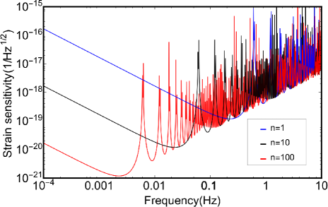
Figure 3: (Color online) Sensitivity curves for $n=1$, $10$, and $100$-trip one-way laser propagation in the presumed absence of acceleration noise.

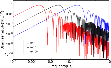
Figure 4: (Color online) The curves for the transfer function with $n=1$, $10$, and $100$.

However, at low frequencies, the main noise is derived from the residual acceleration noise of the free reference masses, which causes the sensitivity to scale as $1/f^{2}$ similar to that analyzed for LISA lhh00 ; dpc11 ; aad12 . As an estimate, we take the spectral density of phase noise contributed by acceleration noise as $S_{pa}\left(f\right)={S_{a}}/{\left(2\pi f\right)^{4}\left(c\tau\right)^{2}}$ lhh00 , where acceleration noise spectrum is at a level of $S_{a}=9\times 10^{-30}m^{2}s^{-4}\mathrm{Hz}^{-1}$.

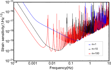
Figure 5: (Color online) Sensitivity curves for $n=1$, $10$, and $100$-trip one-wave laser propagation with acceleration noise included.

The sensitivity curve can be obtained by

$$h_{f}=\sqrt{S_{h}\left(f\right)}=\sqrt{\frac{S_{p}\left(f\right)}{\Gamma\left(f\right)}},$$ (20)

where the spectral density $S_{p}\left(f\right)$ includes contributions from quantum projection noise and acceleration noise, and $S_{h}\left(f\right)$ is derived from the GW signal. The sensitivity curves for $n=1$, $10$, and $100$ are shown in Fig. 5. Indeed, our $n$-way method is found to be capable of improving sensitivity in the low frequency range with its increased transfer function, but it cannot overcome the acceleration noise floor, which leads to the non-ideal improvement. In fact, the frequency at the point of inflection (approximately 3mHz) is determined by the quantum projection noise that is about $\sqrt{N}\sim 10^{-3}$Hz. Thus, our method provides a way to reach the same sensitivity near the inflection point of the frequency with decreased length between two atomic clocks but with increased repeated number of the laser pulses, as presented in Fig. 5 where the case for $n=100$ is equivalent to that for the distance $d=5\times 10^{10}$ m.

V Conclusion

In this paper, we propose a $n$-way scheme of GW detection with optical atomic clocks. At first, we have compared the single two-way measurement or two one-way measurements with the single one-way measurement and found that although two one-way measurements are optimal, but it is not easy to extend to more ways and in particular, its optical measurement cannot shift to lower frequency. So the two-way measurement is focused, since it has an advantage that shifts the optimal measurement to lower frequency, which is a special case ($n=2$) in our recycling scheme. For our method suggested in fourth section, it is found that the signal of $n$-ways summation can improve the sensitivity for low-frequency GW by reducing the quantum projection noise over a broad frequency range. Our method, in essence, is equivalent to the operation of increasing the distance between atomic clocks by increasing the number of the repeated sending pulses within the permission of other operation conditions, i.e. atomic linewidth. This means that if we want to detect lower GW frequencies, we don’t need to set up the scheme by taking a larger distance between atomic clocks, and it can be reached only by repeating to send some pulses back and forth, but the repeated number is limited by the atomic linewidth. This is different from the average over many measurements, since the latter cannot shift the optimal measurement point to lower frequencies. We thus conclude that our $n$-way protocol presents a nice improvement for space-based optical interferometry with baseline length of $10^{8}$ meters, which needs lower optical power compared to those space-based detectors with longer arm length. We have also studied the situation including the acceleration noises and found that the improvement of sensitivity would be restrained below the inflection point of frequency which is determined by the quantum projection noise. So a better method is required to reduce the acceleration noises for the further improvement of sensitivity in the low-frequency GW detection.

VI Acknowledge

We thank Li You for the helpful discussions and insights. This work is supported by NSFC (No. 11654001 and No. 91636213). B. Zhang suggested and planned the work, F. He and B. Zhang finished all analyses and calculations together, and F. He made all the figures.

References

- (1) S. Kolkowitz, I. Pikovsk, N. Langellier, M. D. Lukin, R. L. Walsworth, and J. Ye, Phys. Rev. D 94, 124043 (2016).
- (2) K. S. Thorne, in Three Hundred Years of Gravitation, edited by S. W. Hawking and W. Israel (Cambridge University Press, Cambridge, England, 1987).
- (3) B. P. Abbott and et al., Phys. Rev. Lett. 116, 061102 (2016).
- (4) B. P. Abbott and et al., Phys. Rev. Lett. 116, 241103 (2016).
- (5) B. P. Abbott and et al., Phys. Rev. Lett. 118, 221101 (2017).
- (6) B. P. Abbott and et al., Phys. Rev. Lett. 119, 141101 (2017).
- (7) B. P. Abbott and et al., Phys. Rev. Lett. 119, 161101 (2017).
- (8) P. Amaro-Seoane, S. Aoudia, S. Babak, et al., Classical and Quantum Gravity. 29, 124016 (2012).
- (9) P. Amaro-Seoane, S. Aoudia, S. Babak, et al. arXiv: 1201.3621 [astro-ph].
- (10) LISA: Laser Interferometer Space Antenna for the detection and observation of gravitational waves, Pre-Phase A Report. Max-Planck-Institute, MPQ 208 (1996).
- (11) P. Amaro-Seoane and et al., Class Quantum Grav. 29, 124016, 2012.
- (12) P. Amaro-Seoane and et al. arXiv:1702.00786.
- (13) J. Luo and et al., Class. Quantum Grav. 33, 035010 (2016).
- (14) W. R. Hu and Y. L. Wu, National Science Review 4, 685 (2017).
- (15) D. C. Backer and R. W. Hellings, Ann. Rev. Astro. Astrophys 24, 537 (1986).
- (16) J. Cordes and R. Shannon, arXiv:1010.3785.
- (17) J. W. Armstrong, Living Rev. Relativity 9, E2 (2006).
- (18) https://lisa.nasa.gov/.
- (19) R. F. C. Vessot, et al., Phys. Rev. Lett. 45, 2081 (1980).
- (20) W. J. Kaufmann, Nature 327, 157 (1970).
- (21) R. W. Davies, ”Issues in Gravitational Wave Detection with Space Missions”, in Gravitational Waves and Radiations, Proceedings of the international conference, Université de Paris V, Paris, France, June 18-22, 1973, Colloques Internationaux du CNRS, 220, pp. 33-45, (CNRS, Paris, France, 1974).
- (22) J. C. Breidenthal and T. A. Komarek, “Radio Tracking System,” chapter in Deep Space Telecommunications Systems Engineering (J. H. Yuen, editor), New York: Plenum Press, 1983.
- (23) F. B. Estabrook and H. D. Wahlquist, Gen. Relativ. Gravit. 6, 439 (1975).
- (24) M. Bishof, X. Zhang, M. J. Martin, and J. Ye, Phys. Rev. Lett. 111, 093604 (2013).
- (25) P. W. Graham, J. M. Hogan, M. A. Kasevich, and S. Rajendran, Phys. Rev. Lett. 110, 171102 (2013).
- (26) J. M. Hogan and M. A. Kasevich, Phys. Rev. A 94, 033632 (2016).
- (27) S.-W. Chiow, J. Williams, and N. Yu, Phys. Rev. A 92, 063613 (2015).
- (28) M. A. Norcia, J. R. K. Cline, and J. K. Thompson, Phys. Rev. A 96, 042118 (2017).
- (29) J. Su, Q. Wang, Q. Wang, and P. Jetzer, Class. Quantum Grav. 35, 085010 (2018).
- (30) N. J. Cornish and L. J. Rubbo, Phys. Rev. D 67, 022001 (2003).
- (31) R. Schilling, Classical Quantum Gravity 14, 1513 (1997).
- (32) A. D. Ludlow, M. M. Boyd, J. Ye, E. Peik, and P. O. Schmidt, Rev. Mod. Phys. 87, 637 (2015).
- (33) M. M. Boyd, T. Zelevinsky, A. D. Ludlow, S. M. Foreman, S. Blatt, T. Ido, and J. Ye, Science 314, 1430 (2006).
- (34) M. Tinto, Phys. Rev. D 53, 5354 (1996).
- (35) T. Piran, E. Reiter, W. G. Unruh, and R. F. C. Vessot, Phys. Rev. D 34, 984 (1986).
- (36) S. L. Larson, W. A. Hiscock, R. W. Hellings, Phys. Rev. D 62, 062001 (2000).
- (37) B. Tang, B. Zhang, L. Zhou, J. Wang, and M. S. Zhan, Eur. Phys. J. D 69, 233 (2015).
- (38) H. Guan-Chyun and J. C. Hung, Phase-locked loop techniques. A survey, IEEE Transactions on Industrial Electronics 43, 609 (1996).
- (39) K. Danzmann, T. Prince, P. Binetruy, P. Bender, S. Buchman, J. Centrella, M. Cerdonio, N. Cornish, A. Cruise, C. Cutler et al., LISA: Unveiling a hidden universe, Assessment Study Report ESA/SRE 3, 2 (2011).
- (40) P. Amaro-Seoane, S. Aoudia, S. Babak, P. Binetruy, E. Berti, A. Bohe, C. Caprini, M. Colpi, N. J. Cornish, K. Danzmann et al., Low-frequency gravitational-wave science with eLISA/NGO, Classical Quantum Gravity 29, 124016 (2012).