Framework for Polarized Superfluid Fermion Systems

Abstract

I discuss the advantages and disadvantages of several procedures, some known and some new, for constructing stationary states within the mean field approximation for a system with pairing correlations and unequal numbers spin-up and spin-down fermions, using the two chemical potentials framework. One procedure in particular appears to have significant physics advantages over previously suggested in the literature computational frameworks. Moreover, this framework is applicable to study strongly polarized superfluid fermion systems with arbitrarily large polarizations and with arbitrary total particle numbers. These methods are equally applicable to normal systems.

I Introduction

It is well known that by removing or adding a nucleon from a magic nucleus the self-consistent mean field solution breaks the rotational symmetry and time-odd contributions also appear in the mean field. By adding or removing more nucleons typically nuclei become more deformed in the mean field description and their excited spectra evolve from vibrational to rotational spectra Bohr and Mottelson (1969); Ring and Schuck (2004). One can ask the question: “How a large spin polarization of nuclei, neutron or nuclear matter would modify the properties of their ground states and spectra and their response to various external perturbations?" The interest in spin polarized nuclei, neutron, and nuclear mater is extensive Bauer and Torres Patiño (2020); Polls and Vidana ; Urban and Ramanan (2020); L.Riz et al. ; Stein ; Stein et al. (2016a); Forbes et al. (2014); Tews and Schwenk (2020); Torres Patiño et al. (2019); Behera et al. (2016); Dexheimer et al. (2017); Harutyunyan and Sedrakian (2016); Rabhi et al. (2015); Stein et al. (2016b); Sammarruca et al. (2015); Behera et al. (2015); Vidaña et al. (2016); Lacroix and Bennaceur (2015); Krüger et al. (2015); Aguirre et al. (2014); Bordbar and Rezaei (2013); Dong et al. (2013); Isayev and Yang (2011, 2012); Isayev (2006).

The odd or the odd-odd superfluid nuclei are the simplest examples of spin polarized systems. The definition of a spin polarized system depends on various circumstances. Polarization, in particular the magnetization of condensed matter systems, can be due either to a spontaneous symmetry breaking or it can be induced by an external field. The magnitude of the polarization, or loosely speaking of the difference between the particle numbers with spins up and down $N_{\uparrow}-N_{\downarrow}$ is not as a rule an integer. Moreover, $N_{\uparrow}-N_{\downarrow}\neq 0$ can occur in both normal and superfluid systems. Polarized systems can be also artificially “manufactured” and this is routinely done in cold atom physics.

In a time-dependent framework, a major difficulty in studying the dynamics of a superfluid fermionic system in general or in particular of a nuclear system with an imbalance of spin-up and spin-down fermions ($N_{\uparrow}\neq N_{\downarrow}$), is the construction the initial stationary state needed in time-dependent treatments. Using the simple blocking approximation for the initial state could be problematic in the case of time-dependent phenomena. Within the blocking approximation the odd fermion is often described by a single-particle wave function and not by a Bogoliubov quasiparticle wave function, and thus the orthogonality between the two types of fermion wave functions cannot be enforced during the time evolution, except within the BCS approximation. Using the equal filling approximation, when the extra odd fermion occupation probability is spread uniformly among several levels leads to unphysical polarization properties of the system, which can have major unphysical consequences when describing the nuclear fission of odd or odd-odd nuclei.

Of particular interest is the microscopic description and the understanding of the nuclear fission dynamics, particularly of the stage where the fissioning nucleus emerges from below the potential barrier near the saddle, to the scission configuration. This part of the nuclear evolution is a highly non-equilibrium process, where pairing correlations play the role of a very efficient “lubricant” Bertsch and Bulgac (1997); Bulgac et al. (2019a, 2020). Experiments show that the fission of odd or odd-odd nuclei is hindered significantly when compared to the fission of the neighboring even-even nuclei Vandenbosch and Huizenga (1973); Wagemans (1991). The unpaired fermion(s) can be found in a state with a relatively high total orbital angular momentum projection on the reaction axis and in that case the presence of an odd fermion can have a strong hindering effect, as the pairing correlations, particularly within the traditional theoretical nuclear approaches used so far, are ineffective in the case of the extra nucleon. This is very easy to understand. In the case of an odd or odd-odd heavy nucleus the odd particle(s) can have a very large orbital angular momentum along the symmetry axis $l_{z}\approx\pm p_{F}R\approx 9\hbar$, where $p_{F}$ is the Fermi momentum and $R\approx 1.1A^{1/3}$ is the waist radius of the fissioning nucleus. Such single-particle states are populated for example when studying the induced fission of ²³⁹U obtained in the one-neutron transfer reaction, such as the recently published experimental study ⁹Be(²³⁸U,²³⁹U)⁸Be Ramos et al. (2020). In the fission fragments the maximum angular momentum is expected however to be $l_{z}(H)\approx\pm 7.5\hbar$ and $l_{z}(L)\approx\pm 6.7\hbar$ for the heavy (H) and light (L) fragments respectively, thus smaller by roughly $15\pm 5$% than in the mother nucleus. Since nuclei in the majority of theoretical models used so far are predominantly axially symmetric along the fissioning direction Bender et al. (2004); Ryssens et al. (2015); Schunck and Robledo (2016), when they fission the value of $l_{z}$ of the odd nucleon(s) should be conserved, as the pairing correlations are ineffective in lowering the angular momentum of the extra nucleon or nucleons. This is unlike the case of an even-even nucleus where pairing is very efficient in performing transitions of the type $(j_{z},-j_{z})\rightarrow(j^{\prime}_{z},-j^{\prime}_{z})$ and can thus lower the orbital angular momentum of nucleon pairs Bertsch and Bulgac (1997); Bulgac et al. (2019a, 2020). Clearly the maximum initial $l_{z}\approx\pm 1.1A^{1/3}p_{F}$ and the maximum final values of the odd nucleon(s) in the heavy and light fragments $l_{z}(H,L)\approx\pm 1.1(A_{H,L})^{1/3}p_{F}$ differ vastly, a tension which is usually at the root of the argument why fission of odd and odd-odd nuclei is hindered when compared with the fission of even-even nuclei. The breaking of the axial symmetry obviously can help, but that woulds require some deformation energy. Also collisions, which are neglected in mean field treatments, can also help to transfer several units of angular momentum, but they are Pauli suppressed at low intrinsic excitation energies. Both of these processes are expected to be less efficient that the pairing correlations, which are can be enhanced due to the presence of a pairing condensate Bulgac et al. (2019a, 2020).

One has to remember that the $s$-wave pairing type of matrix elements, which are by design included within a time-dependent Density Functional Theory (DFT) for superfluid systems Bulgac (2013, 2019); Bulgac and Forbes , account for a significant portion of the collision integral at low excitation energies, even in the absence of a true pairing condensate. The main difference between balanced/unpolarized ($N_{\uparrow}=N_{\downarrow}$) and imbalanced/polarized ($N_{\uparrow}\neq N_{\downarrow}$) superfluids is that in the first case the Cooper pairs have zero momentum and the Coopers pairs have a finite momentum in the other case respectively Bulgac and Forbes (2008); Bulgac et al. (2012), a fact known theoretically for a long time in condensed matter systems Larkin and Ovchinnikov (1964); Fulde and Ferrell (1964) and in cold atom physics as well. The presence of Cooper pairs with finite momentum will be instrumental in lowering the orbital angular momentum of the extra nucleons in case of nuclear fission.

One theoretical method used to describe (static) pairing correlations in a system with an odd number of fermions requires the use of two different chemical potentials for the approximately time-reversed single-particle states, for spin-up and spin-down respectively, and was discussed in Refs Bulgac (2007); asl ; Sensarma et al. ; Bulgac and Forbes (2008). The presence of an odd fermion can lead to a relatively weak time-reversal mean field symmetry breaking and to different mean fields for the partners of the Cooper pair, induced by the polarization effects due to the odd fermion. The two chemical potential approach has been used in Refs. Bulgac (2007); Sensarma et al. ; Bulgac and Forbes (2008); Bulgac et al. (2012); Bertsch et al. (2009a); Wlazłowski et al. (2018); Magierski et al. (2019); Tüzemen et al. (2020).

The general approach used to describe odd fermion systems used in nuclear physics Dobaczewski and Dudek (1997); Dobaczewski et al. (2000); Ring and Schuck (2004); Schunck et al. (2017); Bertsch et al. (2009b) has the major disadvantage that one needs to know a priori the quantum numbers of the odd fermion. Robledo and Bertsch (2011) however have shown that a gradient technique approach Ring and Schuck (2004) is apparently free of this difficulty. Sometimes the implementation of the general approach is construed as gain, as one can determine at once a slew of low lying excited states of the odd or of the odd-odd nucleus, even though the computational price is high. While adding a single extra fermion to an even fermion system can appear as a small perturbation $~{}{\cal O}(1/A)$, since the low energy spectrum of odd and odd-odd nuclei is relatively dense, a small perturbation can in principle lead to significant changes of the nuclear mean field.

The question I raise here is: “Can one devise a more transparent and computationally faster framework to describe pairing correlations in odd and odd-odd nuclei in particular and for arbitrary spin-polarizations as well?” Since in unpolarized fermion systems, or in even-even nuclei one treats the spin-up and spin-down fermions identically, naturally there is a need for only one chemical potential for either neutrons or protons. It seems then that since in polarized or odd fermion systems, or in odd and odd-odd nuclei, spin-ups and spin-down clearly experience different mean fields, the introduction of two chemical potentials does not appear to need a justification and it seems like the most natural approach. In the end the framework I describe can handle arbitrary spin-polarizations, not limited to the $|N_{\uparrow}-N_{\downarrow}|=1$ case only, which can be of interest in a number of situations.

In Section II I briefly review the Bogoliubov transformation and the definition of various densities for even and odd fermion numbers. In Section III I review a previously suggested framework for odd fermion systems with axial and parity symmetry Bertsch et al. (2009a), I also introduce a couple of generalizations applicable when an octupole deformation is present, and I discuss their advantages and disadvantages. In Section IV I review the framework designed for cold atom systems, in which case the spin-orbit interaction is absent. In Section V I introduce the optimal two chemical potential framework, which appears to be free of any of the disadvantages of those previously suggested in the literature frameworks for nuclear systems. In the appendix A I discuss various representations of the Pauli spin matrices and in the appendix B I discuss several aspects concerning the numerical implementation.

II Formulation of Bogoliubov transformations for even and odd fermion numbers

First I review the case of a system with an even number of fermions, such as even-even nuclei. The creation and annihilation quasiparticle operators are represented as Ring and Schuck (2004)

$$\alpha_{k}^{\dagger}=\int d\xi\left[u_{k}(\xi)\psi^{\dagger}(\xi)+v_{k}(\xi)\psi(\xi)\right],$$ (1)

$$\alpha_{k}=\int d\xi\left[v_{k}^{*}(\xi)\psi^{\dagger}(\xi)+u_{k}^{*}(\xi)\psi(\xi)\right],$$ (2)

and the reverse relations are

$$\psi^{\dagger}(\xi)=\sum_{k}\left[u^{*}_{k}(\xi)\alpha^{\dagger}_{k}+v_{k}(\xi)\alpha_{k}\right],$$ (3)

$$\psi(\xi)=\sum_{k}\left[v^{*}_{k}(\xi)\alpha^{\dagger}_{k}+u_{k}(\xi)\alpha_{k}\right],$$ (4)

where $\psi^{\dagger}(\xi)$ and $\psi(\xi)$ are the field operators for the creation and annihilation of a particle with coordinates $\xi=({\bm{r}},\sigma)$. The normal number (Hermitian $n=n^{\dagger}$ ) and anomalous (skew symmetric $\kappa=-\kappa^{T}$) densities are

$$n(\xi,\xi^{\prime})=\langle\Phi|\psi^{\dagger}(\xi^{\prime})\psi(\xi)|\Phi\rangle$$

$$=\sum_{k}v_{k}^{*}(\xi)v_{k}(\xi^{\prime})=\sum_{l=n,\bar{n}}v_{l}^{2}\phi_{l}^{*}(\xi)\phi_{l}(\xi^{\prime}),$$ (5)

$$\kappa(\xi,\xi^{\prime})=\langle\Phi|\psi(\xi^{\prime})\psi(\xi)|\Phi\rangle$$

$$=\sum_{k}v_{k}^{*}(\xi)u_{k}(\xi^{\prime})=\sum_{l=n,\bar{n}}u_{l}v_{l}\phi_{l}^{*}(\xi)\phi_{\bar{l}}^{*}(\xi^{\prime}),$$ (6)

$$\int d\xi\phi_{k}^{*}(\xi)\phi_{l}(\xi)=\delta_{kl},$$ (7)

with $u_{l}^{2}+v_{l}^{2}=1$, $0\leq u_{l}=u_{\bar{l}}\leq 1$, $0\leq v_{l}=-v_{\bar{l}}\leq 1$, and $n$ and $\bar{n}$ label the time-reversed states $\phi_{l}(\xi),\phi_{\bar{l}}(\xi)$ in the canonical representation Bloch and Messiah (1962); Ring and Schuck (2004), and where

$$\alpha_{k}|\Phi\rangle=0,\quad\langle\Phi|\alpha_{k}^{\dagger}=0,\quad\langle\Phi|\alpha_{k}\alpha_{l}^{\dagger}|\Phi\rangle=\delta_{kl}.$$ (8)

There is in general no rule on how to separate the quasiparticle operators $\alpha^{\dagger}_{k},\alpha_{k}$ into creation and annihilation ones, and one can rename/interchange any number of them, and declare a number of creation operators annihilation operators and vice versa. This is unlike the field operators $\psi^{\dagger}(\xi),\psi(\xi)$, which are defined with respect to the true vacuum, $\psi(\xi)|0\rangle\equiv 0$. Only by requiring that the quasiparticle vacuum $|\Phi\rangle$ corresponds to the lowest, or often to a local minimum, of the total energy of an average even number of fermions, one can clearly distinguish between creation and annihilation quasiparticle operators.

In the case of an odd number of fermions the ground state is defined as $\alpha^{\dagger}_{\mu}|\Phi\rangle$ Ring and Schuck (2004), where $\mu$ is an appropriately chosen a priori quasiparticle state, and thus

$$\alpha_{l}\alpha_{\mu}^{\dagger}|\Phi\rangle=\delta_{l\mu},\quad\langle\Phi|\alpha_{\mu}\alpha_{k}^{\dagger}=\delta_{k\mu}.$$ (9)

Since by definition $|\Phi\rangle$ corresponds to an average even number of fermions $N$, the state $\alpha^{\dagger}_{k}|\Phi\rangle$ should describe an odd number of fermions $N\pm 1$, and their corresponding particle parity is given by $(-1)^{N}=+1$ or $(-1)^{N\pm 1}=-1$ respectively. Note however, than the state $\alpha^{\dagger}_{k}|\Phi\rangle$, where $|\Phi\rangle$ is defined in Eq. (10), does not automatically has an integer average odd number of fermions, as the chemical potential, and therefore the quasiparticle wavefunctions should be correspondingly adjusted. As

$$|\Phi\rangle\propto\prod_{k}\alpha_{k}|0\rangle,$$ (10)

(assuming that $\alpha_{k}|0\rangle\neq 0$ for any $k$, otherwise see Ring and Schuck (2004)) the ground state of an odd fermion system is therefore defined as

$$\alpha_{l}^{\dagger}|\Phi\rangle\propto\prod_{k\neq l}\alpha_{k}|0\rangle,$$ (11)

where $|0\rangle$ is the particle vacuum, and thus $\psi(\xi)|0\rangle\equiv 0$. The normal number and anomalous densities are in this case

$$n_{l}(\xi,\xi^{\prime})=\langle\Phi|\alpha_{l}\psi^{\dagger}(\xi^{\prime})\psi(\xi)\alpha_{l}^{\dagger}|\Phi\rangle$$

$$=\sum_{k\neq l}v_{k}^{*}(\xi)v_{k}(\xi^{\prime})+u_{l}(\xi)u^{*}_{l}(\xi^{\prime}),$$ (12)

$$\kappa_{l}(\xi,\xi^{\prime})=\langle\Phi|\alpha_{l}\psi(\xi^{\prime})\psi(\xi)\alpha_{l}^{\dagger}|\Phi\rangle$$

$$=\sum_{k\neq l}v_{k}^{*}(\xi)u_{k}(\xi^{\prime})+u_{l}(\xi)v^{*}_{l}(\xi^{\prime}).$$ (13)

Thus the major difference from Eqs. (5-6) is the absence of the contribution of the chosen quasiparticle state $l$ in the sum, which is replaced by the “flipped” quasiparticle wavefunction $(u_{l}(x),v_{l}(x))\leftrightarrow(v^{*}_{l}(x),u^{*}_{l}(x))$. This quasiparticle state $l$ is chosen so as to minimize the total energy of the system with a fixed average odd fermion number. In the case of an odd-odd nucleus one has to naturally chose two such quasiparticle states, one for the neutron and the other for the proton subsystems respectively.

III Self-consistent equations for systems with an odd number of fermions

Here I describe the two chemical potential framework for a polarized (odd) fermion system, assuming axial symmetry, which apparently was first introduced in Ref. Bulgac (2007) and in my argumentation here I follow the line of reasoning of Ref. Bertsch et al. (2009a). I introduce a new quantum number $\eta$, the sign of the expectation value of the single-particle angular momentum operator along the axial symmetry axis $Oz$ and the corresponding operator

$${\cal S}_{z}=\text{sign}({j}_{z})=\text{sign}\left({l}_{z}+\frac{\hbar}{2}\sigma_{z}\right).$$ (14)

If $Oz$ is the axial symmetry axis then the quasiparticle wavefunctions are eigenfunctions of ${\cal S}_{z}$ with eigenvalues

$$\eta=\text{sign}(m)=\pm 1$$ (15)

where $\hbar m$ are the eigenvalues of $j_{z}$. The self consistent equations are:

$$\begin{pmatrix}\text{H}_{\eta\uparrow\uparrow}&H_{\uparrow\downarrow}&0&\Delta\\ H_{\downarrow\uparrow}&\text{H}_{\eta\downarrow\downarrow}&-\Delta&0\\ 0&-\Delta^{*}&-\text{H}^{*}_{\eta\uparrow\uparrow}&-H^{*}_{\eta\uparrow\downarrow}\\ \Delta^{*}&0&-H^{*}_{\eta\downarrow\uparrow}&-\text{H}^{*}_{\eta\downarrow\downarrow}\end{pmatrix} \begin{pmatrix}u_{km,\uparrow}\\ u_{km,\downarrow}\\ v_{km,\uparrow}\\ v_{km,\downarrow}\end{pmatrix}$$

$$={\cal H}_{km}\psi_{km} \begin{pmatrix}u_{km,\uparrow}\\ u_{km,\downarrow}\\ v_{km,\uparrow}\\ v_{km,\downarrow}\end{pmatrix},$$ (16)

$$\text{H}_{\eta\sigma,\sigma}=H_{\sigma\sigma}-\mu-\mu_{\eta}{\cal S}_{z}-Q,\quad\text{with}\quad\sigma=\uparrow,\downarrow,$$ (17)

where $\psi_{km}$ is the four component quasiparticle wave function and where I suppressed the arguments $({\bm{r}},\sigma)$ for spatial and spin coordinates (isospin is not explicitly displayed). $Q=\sum_{l}\lambda_{l}Q_{l0}$ stands for all other necessary constraints, including the corresponding Lagrange multipliers, and $k$ stands for the rest of quantum numbers characterizing the quasiparticle states, apart from $m$. I have also used a short hand notation for the components of the quasiparticle wavefunctions $u_{km,\sigma}=u_{km}({\bm{r}},\sigma),\;v_{km,\sigma}=s_{km}({\bm{r}},\sigma)$, where $\sigma=\uparrow,\downarrow$. In this case there are two chemical potentials $\mu+\eta\mu_{\eta}=\mu\pm\mu_{\eta}$.

The normal partial and total number (and other relevant) densities and also anomalous densities are

$$n_{\eta}({\bm{r}},\sigma,\sigma^{\prime})=\sum_{E_{km}>0}v_{km}^{*}({\bm{r}},\sigma^{\prime})v_{km}({\bm{r}},\sigma)\delta_{\eta,\text{sign}(m)},$$ (18)

$$n({\bm{r}},\sigma,\sigma^{\prime})=n_{+}({\bm{r}},\sigma,\sigma^{\prime})+n_{-}({\bm{r}},\sigma,\sigma^{\prime}),$$ (19)

$$\nu({\bm{r}})=\sum_{E_{km}>0}v_{km}^{*}({\bm{r}},\downarrow)u_{km}({\bm{r}},\uparrow).$$ (20)

The Hamiltonian $H_{\sigma,\sigma^{\prime}}({\bm{r}})$ and the pairing potential $\Delta_{\sigma,-\sigma}({\bm{r}})$ are functional derivatives of the energy density functional (EDF) ${\cal E}(n,\nu,\tau,\ldots)$

$$H_{\sigma,\sigma^{\prime}}({\bm{r}})=\frac{\delta{\cal E}(n,\nu,\tau,\ldots)}{\delta n({\bm{r}},\sigma,\sigma^{\prime})},$$ (21)

$$\Delta_{\sigma,-\sigma}({\bm{r}})=\frac{\delta{\cal E}(n,\nu,\tau,\ldots)}{\delta\nu({\bm{r}},\sigma,-\sigma)}.$$ (22)

Note that $\Delta_{\sigma,\sigma}({\bm{r}})\equiv 0$ in case of $s$-wave pairing and either proton-proton or neutron-neutron pairing. The generalization of the formalism to either $s$-wave proton-neutron pairing or higher partial wave nucleon-nucleon pairing is straightforward. The EDF of nuclear systems typically depends on the sum $n({\bm{r}},\sigma,\sigma^{\prime})=n_{+}({\bm{r}},\sigma,\sigma^{\prime})+n_{-}({\bm{r}},\sigma,\sigma^{\prime})$ alone. In the case of cold atoms the EDF depends on both $n_{\pm}({\bm{r}},\sigma,\sigma^{\prime})$ separately, as fermions of various flavors can reside in different external potentials. This situation is formally equivalent to placing the cold atom system in a strong “magnetic” field, with large “spin-up and spin-down magnetic moments,” see Section IV. The two chemical potentials $\mu\pm\mu_{\eta}$ are determined from the condition that the total and partial particle numbers are

$$N=N_{+}+N_{-},\quad|N_{+}-N_{-}|=1,$$ (23)

$$N_{\pm}=\int d^{3}{\bm{r}}\sum_{\sigma=\uparrow,\downarrow}n_{\pm}({\bm{r}},\sigma,\sigma).$$ (24)

Notice that the equations for the quasiparticle states with $m>0$ ($\eta=+1$) and $m<0$ ($\eta=-1$) respectively have two different chemical potentials $\mu_{\pm 1}=\mu\pm\mu_{\eta}$, and in both cases the eigenvalues $E_{km}$ come also in pairs $(E_{km},-E_{km})$, see also Section IV.

The operator ${\cal S}_{z}$ can be used in the case of axial symmetry for a nucleus with octupole deformation, unlike the hermitian signature operator $i\exp(-i\pi{j}_{x}/\hbar)$ with eigenvalues $\pm 1$ suggested in Ref. Bertsch et al. (2009a).The operator $R_{x}=\exp(-i\pi{j}_{x}/\hbar)=-R_{x}^{\dagger}$ is anti-Hermitian, since $R_{x}^{\dagger}R_{x}=1$ and $R_{x}^{2}=-1$ for a single fermion state. One can relatively easily use instead of the operator $i\exp(-i\pi{j}_{x}/\hbar)$ the so called simplex operator $i\exp(-i\pi{j}_{x}/\hbar)P$ Dobaczewski et al. (2000), where $P$ is the spatial parity operator, if both quadrupole and octupole deformations are present. I find the use of the operator ${\cal S}_{z}$ however much simpler to implement numerically, particularly if one uses a coordinate representation of the quasiparticle wave functions on spatial 3D lattice, see Apendix B. If one uses the operator ${\cal S}_{z}$, then quasiparticle states with $\eta=\text{sign}(m)=\pm 1$ are assigned to particle numbers $N_{\pm}$ and densities $n_{\pm}({\bm{r}},\sigma,\sigma^{\prime})$ respectively.

Another option would be to use the operator $i\exp(-i\pi{j}_{z}/\hbar)=i\exp(-im\pi)=\pm 1$. In this case quasiparticle states with $m=+1/2,-3/2,+5/2,\ldots$ are assigned to particle number $N_{+}$ and $n_{+}({\bm{r}},\sigma,\sigma^{\prime})$, and states with $m=-1/2,+3/2,-5/2,\ldots$ are assigned to particle number $N_{-}$ and $n_{-}({\bm{r}},\sigma,\sigma^{\prime})$, respectively. Time-reversed partners are in both cases assigned to different groups, but using different criteria.

This ambiguity in assigning the quasiparticle states to either one or another partial number density in the case of an odd fermion number is general. One can use any rule to separate quasiparticle states in two groups, and there is no general prescription on how to assign them to specific particle number (aka $``N_{+}$” and “$N_{-}$”) or number densities. The best solution should always correspond to the lowest total energy, which might not always favor the strongest pairing correlations. The many-fermion self-consistent equations never have a unique solution, even for even (in the case of electrons or cold atoms) or even-even nuclei, though only one of them is the lowest total energy. Multiple vacua however, can also correspond to physically realizable states, separated by strong potential barrier, a situation which is quite ubiquitous in quantum field theories or infinite many-body systems, where symmetry is spontaneously broken. The ambiguities I discuss here for odd fermion systems in this sense should not come as a surprise, but merely as new examples of such physically realizable “ground states.” However, since in the case of odd fermion systems the density of low energy levels is relatively high, any such prescription is to some extent arbitrary, and the true ground state might emerge as an optimal superposition of many such quasiparticle vacua, with well defined quantum numbers. One of the simplest examples is that of a system with spontaneous parity breaking, when the ground and the first excited states are separated by an exponentially small energy difference, a phenomenon known in the literature as parity doubling Sheline et al. (1989); Dobaczewski and Engel (2005). Another possibility is that of shape coexistence, see e.g. Refs. Andreyev et al. (2000); Clément et al. (2016) and references therein, of which there are many examples of other types too.

There is still another ambiguity. If both quadrupole and octupole deformations are present in a nucleus with axial symmetry, it is not clear whether the ground state of the nucleus corresponds to either $N_{+}-N_{-}=\pm 1$, and thus whether the projection of the total angular momentum ${J}_{z}(n)=\sum_{n=1}^{A}{j}_{z}(n)\neq 0$ is along or opposite to the fission direction. Such a situation can be experimentally studied in fission induced by a nucleon transfer from an impinging projectile to a nucleon state with relatively large angular momentum Ramos et al. (2020). The projectile will impact an angular momenta perpendicular to the reaction plane equal to either $l_{z}\approx\pm Rk_{F}$. The emergence of the fission fragments emitted along the axis perpendicular to the reaction plane, might favor the emission of the either the light or of the heavy fission fragment in the direction of the impacted angular momentum. It would very interesting to see if any asymmetry of the fission fragments distribution along the direction perpendicular to the reaction plane exists, as such a phenomenon has not been studied yet to my knowledge.

In order to illustrate more vividly the difficulties with the prescriptions described in this section I will apply them to a very simple case, non-interacting “neutrons” in a spherical harmonic oscillator potential with a constant spin-orbit interaction and no pairing field:

$$H=-\frac{\hbar^{2}\Delta}{2m}+\frac{m\omega^{2}{\bm{r}}^{2}}{2}+V{\bm{l}}\cdot{\bm{s}},$$ (25)

as spin-polarization is a property of both normal and superfluid fermionic systems. Since there is no “neutron-neutron” interaction the mean field is independent of the number of particles, and the ground state is typically degenerate for even particle numbers. In Fig. 1 I show the quasi-particle spectra for the two types of constraints discussed in this section

$${H}-\mu_{\eta}{j}_{z}\quad\text{and}\quad{H}-\mu_{\eta}\;\text{sign}({j}_{z}).$$ (26)

Since the Hamiltonian has spherical symmetry the choice of constraining axis is arbitrary.

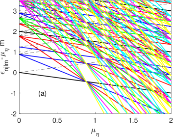
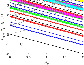
Figure 1: (Color online) The colors for down-sloping quasi-particle levels are black ($l=0$), blue ($l=1$), red ($l=2$), green ($l=3$), magenta ($l-4$), cyan ($l=5$), and yellow ($l=6$) respectively. The corresponding up-sloping levels are always displayed with black dashed thin lines for the sake of the clarity of the figure. In panel (a) are the energy levels for ${H}-\mu_{\eta}{j}_{x}$ and the lower panel for $H-\mu_{\eta}\;\text{sign}({j}_{x}).$ Notice that in panel (b) the states with $j>1/2$ are multiple degenerate and for display purposes only have been artificially perturbed. For example there are three down-sloping $1d_{5/2}$ levels corresponding to $m=1/2,3/2$ and $5/2$. The single-particle energies $\epsilon_{njlm}$, the chemical potential $\mu_{\eta}$ are in units of $\hbar\omega$ and the strength of the spin-orbit interaction was chosen as $V=0.12\hbar\omega$ in these examples.

The two spectra have distinctly different aspects. For small values of $\mu_{\eta}$ one can hastily conclude that either type of constraint apparently leads to desired outcomes. E.g. a system with $N=8$ particles at $\mu_{\eta}=0$ is a closed shell, but for small finite values of $\eta$ a particle is promoted from the $1p_{1/2},m=-1/2$ level to the $1d_{5/2}$ level.

Since the cranking operator is ${j}_{z}$ the net result of such a constraint is imparting the system a net total angular momentum ${J}_{z}=\sum_{i=1}^{N}{j}_{z}(i)$ however, which naturally also gives raise to a spin-polarization. This is clearly seen in the upper panel of Fig. 1 for $\mu_{\eta}\approx 1$, when mostly down-sloping levels with $m>0$ are occupied. The same kind of ground state is obtained also in the case of constraint $\text{sign}({j}_{z}).$ In this case levels with $m>0$ are down-slopping and levels with $m<0$ are up-sloping, all with identical slopes. Nevertheless, the same undesired characteristic of the system ground state is obtained for a highly polarized system. In the case of real nucleus, when the depth of the mean field potential is finite, the radial profiles of the single-particle wave functions are affected in drastically different manners for up-sloping (less bound) and down-sloping (more bound) levels, as a result of a large finite total angular momentum of the system. The system is polarized because it was forced to have a large total angular momentum, as opposed to what one might expected to have a finite total momentum due to the finite popularization of the system. Basically in either of the prescriptions discussed in this section and in Ref. Bertsch et al. (2009a) the roles of the effect and cause have been inadvertently switched. Since a finite spin-polarization of a fermionic system corresponds in the mean field approximation to the breaking of the time-reversal invariance, a finite spin-polarization is always accompanied by a non-vanishing total angular momentum in vice versa. In practice however, one has to clearly distinguish between what kind of constraint one intends to impose, as different constraints lead to different outcomes.

IV The case of fermionic polarized cold atom systems

In the case of cold atoms one has two flavors of fermions, which I shall denote with $a$ and $b$, and the Cooper pair is formed between one fermion $a$ with another fermion $b$. Entangled states, when for example a type $a$ fermion can coexist with a type $b$ fermion, in a type of the Schrödinger cat single-particle state, have not been studied yet, neither experimentally nor theoretically to my knowledge. Only the formation of Copper pairs between a type $a$ fermion and a type $b$ fermion have been considered so far in the literature. Such a mixing is formally similar to the spin-orbit coupling of the nucleon motion in nuclei, and it will be illustrated qualitatively in Fig. 2. In the absence of such mixing the mean field equations read Bulgac (2007); Sensarma et al. ; Bulgac and Forbes (2008); Bulgac et al. (2012); asl :

$$\begin{pmatrix}H_{a}-\mu_{a}&0&0&\Delta\\ 0&H_{b}-\mu_{b}&-\Delta&0\\ 0&-\Delta^{*}&-H^{*}_{a}+\mu_{a}&0\\ \Delta^{*}&0&0&-H^{*}_{b}+\mu_{b}\end{pmatrix}\begin{pmatrix}u_{k}^{(a)}\\ u_{k}^{(b)}\\ v_{k}^{(a)}\\ v_{k}^{(b)}\end{pmatrix}$$

$$={\cal H}\begin{pmatrix}u_{k}^{(a)}\\ u_{k}^{(b)}\\ v_{k}^{(a)}\\ v_{k}^{(b)}\end{pmatrix}=E_{k}\begin{pmatrix}u_{k}^{(a)}\\ u_{k}^{(b)}\\ v_{k}^{(a)}\\ v_{k}^{(b)}\end{pmatrix}.$$ (27)

where the two chemical potentials $\mu_{a,b}$ are chosen by fixing the particle numbers

$$N_{a,b}=\sum_{E_{k}>0}\int d^{3}{\bm{r}}|v_{k}^{(a,b)}({\bm{r}})|^{2}.$$ (28)

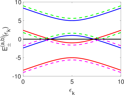
Figure 2: The quasiparticle spectrum $E_{k,\pm}^{(a)}$ (33) with blue and $E_{k,\pm}^{(b)}$ (34) with red lines respectively. The densities are constructed from quasiparticle states with $E_{k,\pm}^{(a,b)}>0$ only. For a finite spin-polarization the quasiparticle states corresponding to the red line with $E_{k,+}^{(b)}>0$. At the same time the fermions of kind $a$ occupy quasiparticle states corresponding to the blue lines with $E_{k,\pm}^{(a)}>0$. The effect of a non-vanishing mixing between the two flavors or of a spin-orbit coupling (characteristic to nuclear systems) on the quasiparticle spectrum is illustrated with dashed lines. In the case of cold atoms this type of mixing is equivalent to the creation of a Schrödinger cat fermion state between type $a$ and type $b$ flavors.

These equations obviously decouple and since in case of cold atoms one typically has $H_{a,b}=H_{a,b}^{*}$, the equations simplify. By introducing

$$H_{\pm}=\frac{H_{a}\pm H_{b}}{2}$$ (29)

these equations can be re-written as

$$\begin{pmatrix}H_{+}-\mu&\Delta\\ \Delta^{*}&-H_{+}+\mu\end{pmatrix}\begin{pmatrix}u_{k}^{(a)}\\ v_{k}^{(b)}\end{pmatrix}$$ (30)

$$=\begin{pmatrix}E_{k}^{(a)}-(H_{-}-\mu_{\eta})&0\\ 0&E_{k}^{(a)}-(H_{-}-\mu_{\eta})\end{pmatrix}\begin{pmatrix}u_{k}^{(a)}\\ v_{k-}^{(b)}\end{pmatrix},$$

$$\begin{pmatrix}H_{+}-\mu&-\Delta\\ -\Delta^{*}&-H_{+}+\mu\end{pmatrix}\begin{pmatrix}u_{k}^{(b)}\\ v_{k}^{(a)}\end{pmatrix}$$ (31)

$$=\begin{pmatrix}E_{k}^{(b)}+(H_{-}-\mu_{\eta})&0\\ 0&E_{k}^{(b)}+(H_{-}-\mu_{\eta})\end{pmatrix}\begin{pmatrix}u_{k}^{(b)}\\ v_{k}^{(a)}\end{pmatrix},$$

and now one can disentangle the different roles operators $H_{+}-\mu$ and $H_{-}-\mu_{\eta}$ play on acting on quasiparticle wave functions. The chemical potentials $\mu$ and $\mu_{\eta}$ are defined in a similar manner

$$\mu=\frac{\mu_{a}+\mu_{b}}{2},\quad\mu_{\eta}=\frac{\mu_{a}-\mu_{b}}{2}.$$ (32)

The self-consistent equations in the nuclear case can be brought to a similar form. Assuming that $H_{a,b}=\varepsilon_{a,b}$ and $\Delta$ are diagonal one can show that

$$E_{k,\pm}^{(a)}=+e_{-}\pm\sqrt{\epsilon_{k}^{2}+|\Delta|^{2}},$$ (33)

$$E_{k,\pm}^{(b)}=-e_{-}\pm\sqrt{\epsilon_{k}^{2}+|\Delta|^{2}},$$ (34)

$$e_{-}=\frac{\varepsilon_{a}-\varepsilon_{b}}{2}-\mu_{\eta},\quad\epsilon_{k}=\frac{\varepsilon_{a}+\varepsilon_{b}}{2}-\mu.$$ (35)

Clearly all eigenvalues come in pairs $E_{k,\pm}^{(a)}=-E_{k,\mp}^{(b)}$. For each eigenvector $(u^{(a)}_{k},v^{(b)}_{k})$ and corresponding eigenvalue $E_{k,\pm}^{(a)}$ of Eq. (30) the Eq. (31) has a corresponding eigenvector $(u^{(b)}_{k},v^{(b)}_{k})=(v^{(a)}_{k},u^{(b)}_{k})^{*}$ and a corresponding eigenvalue $E_{k,\mp}^{(b)}=-E_{k,\pm}^{(a)}$.

As branches of the quasiparticle spectrum are displaced in opposite directions, when part of the lower branch $E^{(a)}_{k,-}$ becomes positive (with blue in Fig.2) and the upper branch $E^{(b)}_{k,+}$ becomes negative (with red in Fig.2), the roles of the components of the Bogoliubov quasiparticles change exactly as discussed in Section II, see Eqs. (12, 13). If $N_{a}-N_{b}$ quasiparticle energies $E_{k,-}^{(a)}$ change their signs, then the new quasiparticle vacuum corresponds to $\prod_{l=1}^{N_{a}-N_{b}}\alpha_{\mu_{l}}^{\dagger}|\Phi\rangle$ and a particle parity $(-1)^{N_{a}-N_{b}}$, where $|\Phi\rangle$ is a total fermion function for an unpolarized system, and $\mu_{l}$ are the corresponding quantum numbers of the positive $E_{k,-}^{(a)}$ quasiparticle states.

When the branches of $E_{k,-}^{(a)}$ and $E_{k,+}^{(b)}$ cross zero, some of the quasiparticles energies could vanish identically, as in the case of bound states on a superfluid vortex line first discussed by Caroli et al. (1964) and have a character similar to Majorana particles. In such a case the fermion system is technically a topological one, characterized by a Chern number associated with the Berry connection and curvature Thouless et al. (1982).

V My favorite two chemical potentials framework for a polarized superfluid Fermi system

Likely the best option is to formulate the two chemical potentials framework for nuclei along the same lines as for the scheme suggested for cold atoms, see Refs. Bulgac (2007); Sensarma et al. ; Bulgac and Forbes (2008); Bulgac et al. (2012) and Section IV. The main difference between nuclei and cold atom systems is in the presence of the spin-orbit interaction in nuclei and the need to introduce the total single-particle angular momentum ${\bm{j}}={\bm{l}}+{\bm{s}}$, where ${\bm{l}}$ is the orbital angular momentum and ${\bm{s}}=\hbar{\bm{\sigma}}/2$ is the nucleon spin, and the spin-orbit interaction, which mixes the spin-up and spin-down states, which is qualitatively different situation from the cold atom case discussed in the previous Section IV. (

The main problem with either the method suggested by Bertsch et al. (2009a) and briefly described in Section III or the “improvement” suggested by me in the same section is that either the constraining operators ${\cal S}_{x,z}$ lead to polarization, exactly as any rotation with a finite frequency would do or a strong magnetic field also induce. The goal is not to bring the nucleus into rotation, and thus excite it, but rather to keep the odd or odd-odd nucleus in its ground state at a given spin-polarization in the mean field approximation. The question arises then, what is the most appropriate constraining operator?

When $\exp\left(-i2\pi{\bm{j}}\cdot{\bm{n}}/\hbar\right)$ is acting on a $1/2$-spinor wave function it changes its sign. The rotation operator can be factorized, since $[{{\bm{l}},{\bm{s}}}]=0$

$$\exp\left(-i\alpha\frac{{\bm{j}}\cdot{\bm{n}}}{\hbar}\right)=\exp\left(-i\alpha\frac{{\bm{l}}\cdot{\bm{n}}}{\hbar}\right)\exp\left(-i\alpha\frac{{\bm{s}}\cdot{\bm{n}}}{\hbar}\right),$$ (36)

where ${\bm{n}}=(\sin\beta\cos\gamma,\sin\beta\sin\gamma,\cos\beta)$ is an arbitrary unit vector. If one considers now separately the action of $\exp(-i2\pi{\bm{l}}\cdot{\bm{n}}/\hbar)$ on any component of the spinor, that component does not change sign. However, when acting with $\exp\left(-i2\pi{\bm{s}}\cdot{\bm{n}}/\hbar\right)$ alone on the $1/2$-spinor wave function, the spatial part of the wave function is obviously unaffected, but the whole spinor wave function changes sign. That allows us to define the operator

$${\cal P}_{N}(\alpha)=\prod_{k=1}^{N}\exp\left[-i\alpha\frac{{\bm{s}}(k)\cdot{\bm{n}}}{\hbar}\right],$$ (37)

where the product runs over all particles. The action of this operator leads to an apparently new and simple representation of the particle parity operator for an $N$-fermion system

$${\cal P}_{N}(2\pi)|\Phi\rangle=(-1)^{N}|\Phi\rangle.$$ (38)

It is particularly easy to check that $\langle\Phi|{\cal P}_{N}(2\pi)|\Phi\rangle\equiv(-1)^{N}$ in the case of a Slater determinant. Since the spin direction can be chosen arbitrarily, this representation of the particle projection operator is clearly not unique and one can use ${\bm{n}}=(0,0,1)$. Exactly as in the case described in Section III the single-particle operator ${\cal P}_{1}(\alpha)=\exp(-i\alpha{\bm{s}}\cdot{n}/\hbar)$ has the obvious properties

$${\cal P}^{\dagger}_{1}(\alpha){\cal P}_{1}(\alpha)=1,\quad{\cal P}_{1}^{2}(\pi)={\cal P}_{1}(2\pi)=-1$$ (39)

and all the argumentation presented in Section III and in Ref. Bertsch et al. (2009a) follows, however, without some of the limitations discussed in Section III and other limitations discussed in Appendix B.

A polarized Fermi system is spin polarized, similarly to the well studied cold atom systems Bulgac (2007); Bulgac and Forbes (2008); Sensarma et al. ; Bulgac et al. (2012); Wlazłowski et al. (2018); Tüzemen et al. (2020); Magierski et al. (2019) or magnetized electron systems for example. If there are no non-vanishing time-odd external or components of the mean field one can show that the ground state of an even-even nucleus has a vanishing total spin $\langle\Phi|\sum_{k=1}^{N}{\bm{s}}(k)|\Phi\rangle\equiv 0$ Vautherin and Brink (1972). Hence, following the same argumentation presented in Ref. Bertsch et al. (2009a) and in Section III, for a polarized fermion superfluid system Eqs. (16, 17) can be rewritten as follows:

$$\begin{pmatrix}\text{H}_{\eta\uparrow\uparrow}&H_{\uparrow\downarrow}&0&\Delta\\ H_{\downarrow\uparrow}&\text{H}_{\eta\downarrow\downarrow}&-\Delta&0\\ 0&-\Delta^{*}&-\text{H}^{*}_{\eta\uparrow\uparrow}&-H^{*}_{\eta\uparrow\downarrow}\\ \Delta^{*}&0&-H^{*}_{\eta\downarrow\uparrow}&-\text{H}^{*}_{\eta\downarrow\downarrow}\end{pmatrix} \begin{pmatrix}u_{k,\uparrow}\\ u_{k,\downarrow}\\ v_{k,\uparrow}\\ v_{k,\downarrow}\end{pmatrix}$$

$$={\cal H}\begin{pmatrix}u_{k,\uparrow}\\ u_{k,\downarrow}\\ v_{k,\uparrow}\\ v_{k,\downarrow}\end{pmatrix}=E_{k} \begin{pmatrix}u_{k,\uparrow}\\ u_{k,\downarrow}\\ v_{k,\uparrow}\\ v_{k,\downarrow}\end{pmatrix},$$ (40)

$$\text{H}_{\eta\sigma,\sigma}=H_{\sigma\sigma}-\mu-\eta\mu_{\eta}-Q,$$ (41)

with $\eta=(\sigma_{z})_{\sigma,\sigma}=\pm 1$ for $\sigma=\uparrow,\downarrow$ respectively. Here I have replaced either the operator ${\cal S}_{z}$ introduced in Section III, or the operator $i\exp(-i\pi{j}_{x}/\hbar)$ introduced by  Bertsch et al. (2009a), or the alternative simplex operator $i\exp(-i\pi{j}_{x}/\hbar)P$ Dobaczewski et al. (2000), both of them discussed in Section III, with the much simpler Hermitian operator $i{\cal P}_{1}(\pi)=i\exp(-i\pi\sigma_{z}/2)\equiv\sigma_{z}$. Then the number densities, the particle numbers, and the anomalous density are determined as follows

$$n_{\sigma}({\bm{r}})=\sum_{E_{k}>0}v_{k}^{*}({\bm{r}},\sigma)v_{k}({\bm{r}},\sigma),\quad\sigma=\uparrow,\downarrow,$$ (42)

$$n({\bm{r}})=n_{\uparrow}({\bm{r}})+n_{\downarrow}({\bm{r}}),$$ (43)

$$N=N_{\uparrow}+N_{\downarrow},\quad N_{\uparrow,\downarrow}=\int d^{3}{\bm{r}}n_{\uparrow,\downarrow}({\bm{r}}),$$ (44)

$$\nu({\bm{r}})=\sum_{E_{k}>0}v_{k}^{*}({\bm{r}},\downarrow)u_{k}({\bm{r}},\uparrow).$$ (45)

The chemical potentials $\mu_{\uparrow,\downarrow}=\mu\pm\mu_{\eta}$ are chosen so as fix both the total particle number $N$ and the degree of spin-polarization $N_{\uparrow}-N_{\downarrow}$. Since the chemical potential $\mu_{\eta}$ enters in the self-consistent equations Eq. (40) as $\mu_{\eta}\sigma_{z}$ the single-particle angular momentum ${j}_{z}$ still commutes with the quasiparticle Hamiltonian ${\cal H}$ for an axially symmetric nucleus. However, a spin polarized odd or odd-odd nucleus strictly speaking cannot be strictly spherical anymore in the mean field approximation, as $[{\bm{j}}^{2},\sigma_{z}]\neq 0$.

Naturally, the same procedure can be used for a nucleus without pairing correlations. The chemical potential $\eta\mu_{\eta}$ act as a fictitious magnetic field $B|\mu_{N}|=\mu_{\eta}$ in case of neutral particles. Consider for example the case of $N$ fermions occupying a set of (ordered) single-particle levels $\varepsilon_{k}$, all with Kramers degeneracies. By applying the “external field” $\mu_{\eta}>(\varepsilon_{N}-\varepsilon_{1})/2$ the system is completely polarized and partially polarized for smaller values of $\mu_{\eta}$.

By placing a nucleus in an external magnetic field of arbitrary magnitude one can also obtain non-vanishing spin-polarizations. However, protons will respond more strongly to a magnetic field, due to their finite orbital magnetic moment. Neutrons and protons cannot be controlled independently in the present framework, as various applications might require, for example when there is a multi-nucleon transfer reaction and one can populate various proton and neutron single-particle states.

The quasiparticle spectrum is not affected qualitatively by the presence or absence of the spin-orbit interaction, see Fig. (2). Notice that in these formulas I have dropped the additional subscript $m$ for the energies and the quasiparticle wave functions, as there is no need for singling out $m$. Various branches of the quasiparticle spectrum are shifted upwards and downwards, see Fig. (2), and the quasiparticle wave functions corresponding to the lowest energies are automatically “flipped” when these quasiparticle energies change sign, see the discussion in previous Sections II, III, and IV.

In the traditional approach used for odd fermion systems, see Refs. Ring and Schuck (2004); Dobaczewski and Dudek (1997); Schunck et al. (2017); Bertsch et al. (2009b) and Section II the quantum numbers for the singled out quasiparticle state $l$, see Eq. (11), are a priori unknown. In order to determine the ground state one needs to perform many simulations with various choices of quantum numbers for quasiparticle state $l$ Schunck et al. (2017); Bertsch et al. (2009b). In this latest formulation, c.f. Eqs. (40), one needs only to specify the degree of spin-polarization $N_{\uparrow}-N_{\downarrow}$ of the system only. $|N_{\uparrow}-N_{\downarrow}|$ could be any integer in principle and therefore in this framework one can generate two or more quasiparticle excited states as well when needed. One can even consider $N_{\uparrow}-N_{\downarrow}$ as any real number and consider fractional total particle numbers Dreizler and Gross (1990), similarly to what has been done in the case of cold atom systems for arbitrary spin-polarizations, and where the agreement of the EDF approach with ab initio quantum Monte Carlo calculations of inhomogeneous systems and also with experiments was excellent Bulgac (2007); Bulgac and Forbes (2008); Bulgac et al. (2012, 2014); Wlazłowski et al. (2015). $N_{\uparrow}-N_{\downarrow}$ can take any value in both even and odd nuclei, a situation which might be very useful when analyzing nuclei in extremely strong magnetic fields, e.g. in magnetars.

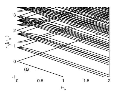
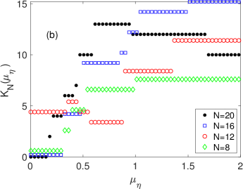
Figure 3: (Color online) The eigenvalues $\epsilon(\eta)$ of the constrained Hamiltonian $H-\mu_{\eta}\sigma_{z}$, with $h$ given by Eq. (25), are shown in panel (a). The corresponding projection of the total angular momentum along the symmetry axis $K_{N}(\mu_{\eta})=\langle\Psi(\mu_{\eta})|\sum_{i=1}^{N}{j}_{x}(i)|\Psi(\mu_{\eta})\rangle$ for a “neutron” with $N=8,12,16$ and 20 particles system is shown in panel (b). $\Psi(\mu_{\eta})$ is the ground state Slater determinant. For visual clarity $K_{N}(\mu_{\eta})$ for different $N$ have been slightly shifted in the vertical direction for better visualization. The energies, $\mu_{\eta}$, and the angular momentum are in units of $\hbar\omega$ and $\hbar$ respectively. $N=8$ and 20 are magical numbers, and $N=16$ as zero spin-polarization corresponds to a complete filling of the $1s_{1/2},1p_{3/2},1p_{1/2},1d_{5/2},2s_{1/2}$ levels and at $\mu_{\eta}\equiv 0$ have $K_{N}(0)=0$ and also $\Sigma_{N}(0)\equiv 0$ as expected, see Fig 4.

I will present now a second argument in favor of the type of constraint discussed in this section. For any nucleus one can consider the generalized number density for one kind of nucleons

$$n_{\sigma,\sigma^{\prime}}({\bm{r}})=\sum_{E_{k}>0}v_{k}({\bm{r}},\sigma)v_{k}^{*}({\bm{r}},\sigma^{\prime}).$$ (46)

Vautherin and Brink (1972) observed that time-reversal invariance implies that for an even-even nucleus in the ground state

$$n_{\sigma,\sigma^{\prime}}({\bm{r}})\equiv\frac{1}{2}\delta_{\sigma,\sigma^{\prime}}n({\bm{r}}),$$ (47)

$$\sum_{\sigma,\sigma^{\prime}}n_{\sigma,\sigma^{\prime}}({\bm{r}}){\bm{\sigma}}_{\sigma^{\prime},\sigma}\equiv 0.$$ (48)

For an odd-odd or odd nucleus that is not true anymore, as clearly that also holds true for excited states of an even-even nucleus with a finite total spin-polarization, when

$${\bm{\Sigma}}_{N}=\int d^{3}r\sum_{\sigma,\sigma^{\prime}}n_{\sigma,\sigma^{\prime}}({\bm{r}}){\bm{\sigma}}_{\sigma^{\prime},\sigma}\neq 0$$ (49)

is non-vanishing. Obviously

$$\int d^{3}r\sum_{\sigma}n_{\sigma,\sigma}({\bm{r}})=N$$ (50)

is the total number of either neutrons or protons. Without any loss of generality one can choose ${\bm{\Sigma}}=(0,0,\Sigma)$ and then one can easily see that for any nucleus

$$N_{\sigma}=\int d^{3}rn_{\sigma,\sigma}({\bm{r}}),\quad\textrm{for}\quad\sigma=\uparrow,\downarrow,$$ (51)

in agreement with Eqs. (42,43,44). Obviously the spin-polarization $\Sigma_{N}$ has always values in a finite interval

$$\Sigma_{N}\in[-N,N]$$ (52)

and in case of nuclear systems one can consider only non-negative values for $\Sigma_{N}$.

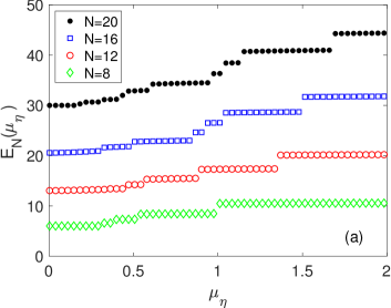
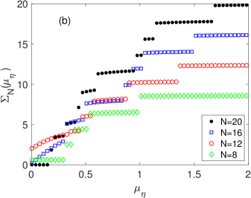
Figure 4: (Color online) The total energy $E_{N}(\mu_{\eta})$ of a normal polarized $N=8,12,16$ and $20$ non-interacting “neutron” system with Hamiltonian (25) is shown in panel (a) as a function of $\mu_{\eta}$ and the total spin-polarization ${\bm{\Sigma}}_{N}(\mu_{\eta})$, see Eq. (49), is shown in panel (b). For visual clarity $\Sigma_{N}(\mu_{\eta})$ for different $N$ have been slightly shifted in the vertical direction for better visualization. Energy and $\mu_{\eta}$ are in units of $\hbar\omega$.

I will compare now the results of imposing this type of constraint on the system discussed at the end of Section (III), see Eq. (25). Figs. 3 and 4 summarize the results for quasi-particle energies $\epsilon_{n}(\mu_{\eta})$ for the constrained Hamiltonian $H-\mu_{\eta}\sigma_{z}$ and for the projection of the total angular momentum along the symmetry axis, energy, and spin-polarization respectively $K_{N}(\mu_{\eta}),E_{N}(\mu_{\eta})$ and $\Sigma_{N}(\mu_{\eta})$ for the total particle numbers $N=8,12,16$ and 20. In Fig. 5 for these values of $N$ I display the dependence of $E_{N}(\Sigma)$, $K_{N}(\Sigma)$, and the “yrast line” $E(K)$ versus $K$. The total angular momentum, the total energy, and the total spin-polarization change by jumps at each quasi-particle level crossing. The total spin-polarization $\Sigma_{z}(\mu_{\eta})$ changes in jumps of $\approx 2$ as expected at each value of $\eta$ where a quasi-particle level crossing occurs, see Fig. 3. There is a glaring difference between the maximum total angular momentum obtained at maximum spin-polarization in Fig. 1 for the constraints $H-\mu_{\eta}{j}_{z}$ and $H-\mu_{\eta}\,\text{sign}({j}_{z})$ and the corresponding value in Fig. 3 corresponding to the constraint $H-\mu_{\eta}\sigma_{z}$. For $N=20$ one obtains at $\mu_{\eta}=1$ the values 64 and 17, and 96 and 25 for $\mu_{\eta}=2$ respectively for the type of constraints discussed in Section III. These values should be compared to the maximum value $K_{N}(\mu_{\eta})\approx 13$ and lower values for the $N=20$ “neutron” system for large values of $\eta$ in Fig. 3. Note that $K_{N}(\mu_{\eta})$ is not a monotonous function of $\mu_{\eta}$, see Fig. 3. One can now better appreciate the difference between enforcing a constraint either on ${j}_{z}$ or on $\text{sign}({j}_{z})$, which imparts a relatively large angular momentum to the system, while also by default leading to its spin-polarization. The spin-polarization of the system obtained in this manner is an effect caused by the finite angular momentum, per discussion in Section III. For each $N$ the system reached it maximum possible spin-polarization $\Sigma_{\text{max}}=|N_{\uparrow}-N_{\downarrow}|=N$. The constraint on $\sigma_{z}$ is directly related to the generalized density $n_{\sigma,\sigma^{\prime}}({\bm{r}})$, which is naturally related to $N_{\sigma}=\int d^{3}r\;n_{\sigma,\sigma}({\bm{r}})$ and thus to the spin-polarization of the system $\Sigma=|N_{\uparrow}-N_{\downarrow}|$. In this case the finite spin-polarization, namely the cause, induces a finite total angular momentum, which is thus an effect.

While the many-body states thus obtained are characterized by axial symmetry, and thus by a good value of the projection of the total angular momentum on the symmetry axis, these states break rotational invariance, as these states do not have a well defined total angular momentum. But so do Slater determinants, formed with single-particle wave functions from an open shell One can denote these states $K\Sigma$-isomers and after angular momentum projection Ring and Schuck (2004) one can restore the rotational symmetry. The spin asymmetry $\Sigma$ along the system symmetry axis is not affected by angular momentum projection, similarly to the $K$ quantum number, since $[j_{z},\sigma_{z}]=0$ and $[\sum_{k=1}^{N}j_{z}(k),\sum_{l=1}^{N}\sigma_{z}(l)]=0$. Notice, see Figs. 3, 4, and 5, that even though $\Sigma$ does not necessarily acquire integer values always, it is in a matter of speaking “quantized,” as it changes by clearly defined jumps. It would be interesting to establish to what extent these kind of $\Sigma$-jumps survive upon the onset of pairing correlations. These $K\Sigma$-isomers are by construction the lowest states characterized by a good quantum number $K$ and a defined spin-asymmetry.

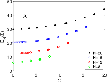
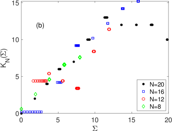
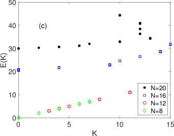
Figure 5: (Color online) The total energy $E_{N}(\Sigma)$ in panel (a), the projection of the total angular momentum $K_{N}(\Sigma)$ along the symmetry axis, and the ‘yrast lines” $E(K)$ versus $K$, all for $N=8,12,16$, and 20 are shown in panel (c). Energy is in units of $\hbar\omega$ and the angular momentum in units of $\hbar$. For visual clarity $K_{N}(\mu_{\eta})$ for different $N$ have been slightly shifted in the vertical direction for better visualization.

VI Conclusions

I discussed here several frameworks suggested in the literature, as well as a few new ones, designed to treat odd fermion superfluid systems, their advantages and disadvantages, and I introduced a two chemical potential framework Bulgac (2007); asl ; Sensarma et al. ; Bulgac and Forbes (2008), which appears to be much simpler to implement in comparison with other frameworks suggested so far in the nuclear physics literature.

Unlike the general framework designed by Dobaczewski and Dudek (1997), which requires an a priori knowledge of the quantum numbers characterizing the extra add fermion, the two chemical potentials framework outlined in Section V and when properly numerically formulated, see Appendix B, eschews the diagonalization of the quasiparticle Hamiltonian, used in order to arrive at a self-consistent solution, and also the need to identify a priori the quantum numbers of the extra fermion. The contribution of the lowest energy quasiparticle state of the odd fermion is automatically selected in this framework, particularly when the simulated annealing method is also incorporated in the iterative process. The gradient method advocated by Robledo and Bertsch (2011) apparently also does not require a priori identification of the quantum numbers of the odd fermion, a method limited however only to the ground states of odd or odd-odd nuclei. The two chemical approach as described here can prove to be essential in constructing the initial states in an induced fission process of a nucleus produced in a many-nucleon transfer reaction, when the state of spin-polarization can be arbitrary. One can also generalize the approach in a straightforward manner to impose both a finite spin-polarization and a total angular momentum as well, to obtained what I have called above  $K\Sigma$-isomers. Since the spin-polarization $\Sigma$ can be “quantized,” the identification of $K\Sigma$-isomers can lead to a deeper understanding of nuclear dynamics, e.g. in fission, and of the properties of nuclear spectra, in a manner analogous to the role played by $K$-isomers.

At this time it is not clear whether either the simulated annealing method or the gradient method Robledo and Bertsch (2011) for generating the new mean field during the iterative process is superior computationally, or even if a carefully combination of the simulated annealing with the gradient method could prove to be the best choice. Since there exists methods Jin et al. (2017); Kashiwaba and Nakatsukasa (2020) which eschew the ubiquitous diagonalization of the quasiparticle Hamiltonian used routinely in the literature, these methods can and should be used in conjunction with simulated annealing and/or gradient methods, in the mean field calculations of polarized fermion systems and then one can achieve a significant numerical speed-up. The framework described here is formally identical to describing nuclei in the presence of strong magnetic fields, which one can encounter in magnetars for example. In the presence of arbitrary strong magnetic fields one can fully polarize a nucleus.

I have conjectured that by studying the asymmetry of the fission fragments distributions, emitted along the direction of the angular momentum of the fissioning odd or odd-odd nucleus one could shed new light on whether time-odd mean field components play a qualitative new role in fission. Compound states in fissioning nuclei with relatively large angular momenta can be populated in one or many neutron transfer reactions Ramos et al. (2020).

Similar, but not identical, type of correlations have been recently analyzed within the phenomenological model CGMF Becker et al. (2013) based on the Hauser-Feshbach framework Hauser and Feshbach (1952) by Lovell et al. (2020) in neutron induced fission of actinides. These authors, while pointing to quite a number of experimental results, observe that with the increasing energy of the incident neutron the anisotropy for the reaction U²³⁸(n,f) is noticeably more pronounced than for the reactions U²³⁵(n,f) and Pu²³⁹(n,f). This analysis thus suggests that fission is favored along the direction of the total angular momentum of the compound nucleus. This type of anisotropy has been postulated by Bohr (1956). It is not clear yet however, whether the emission of the heavy fission fragment is favored or hindered over the emission of the light fission fragment along the direction of the total angular momentum of the compound nucleus.

VII acknowledgement

I thank G.F. Bertsch for a stimulating discussion and I. Stetcu for me making me aware of the recent phenomenological study of fission fragments anisotropy Lovell et al. (2020). I also thank J.E. Drut for making a number of useful suggestions on the manuscript. The work was supported by U.S. Department of Energy, Office of Science, Grant No. DE-FG02-97ER41014 and in part by NNSA cooperative agreement DE-NA0003841.

Appendix A Representation of the Pauli matrices

There is a formal aspect that is hardly ever discussed in the literature, the choice of the three axes for the spin and their relation with the actual spatial directions. It is easy to verify that the Schrödinger equation for a spin particle is invariant with respect to the choice of the spin basis set, which is not the case in the case of cold atom systems. Namely the Schödinger equation does not change if one replaces the canonical Pauli matrices with the new Pauli matrices $\tilde{\bm{\sigma}}$

$$\tilde{\bm{\sigma}}=\exp\left(-i\frac{\kappa}{2}{\bm{\sigma}}\cdot{\bm{m}}\right){\bm{\sigma}}\exp\left(i\frac{\kappa}{2}{\bm{\sigma}}\cdot{\bm{m}}\right),$$ (53)

where ${\bm{m}}=(\sin\chi\cos\zeta,\sin\chi\sin\zeta,\cos\chi)$ is an arbitrary 3D unit vector and ${\bm{\sigma}}$ are the canonical Pauli matrices. The arbitrary angles $\kappa,\chi,\zeta$ have no relation with the usual Euler angles $\psi,\theta,\phi$ describing a rotation in the usual 3D space. Basically what this means is that the particular choice of $\tilde{\sigma}_{z}$ as a diagonal traceless Hermitian matrix is not unique, and any traceless $2\times 2$ Hermitian matrix with eigenvalues $\pm 1$ is an equally acceptable choice. The same applies for the other two Pauli matrices $\tilde{\sigma}_{x,y}$, with the only requirement that

$$[\tilde{\sigma}_{k},\tilde{\sigma}_{l}]=2i\varepsilon_{klm}\tilde{\sigma}_{m},$$ (54)

where $k,l,m=x,y,z$ and $\varepsilon_{klm}$ is the Levi-Civita symbol. One example of a different choice for the Pauli spin matrices different from the canonical one is

$$\tilde{\sigma}_{x}=\begin{pmatrix}0&-i\\ i&0\end{pmatrix},\; \tilde{\sigma}_{y}=\begin{pmatrix}1&0\\ 0&-1\end{pmatrix},\; \tilde{\sigma}_{z}=\begin{pmatrix}0&1\\ 1&0\end{pmatrix},$$ (55)

or any other even permutation of $\sigma_{x,y,z}$. One can choose also an odd permutation, but then the sign of one of the matrices has to be changed. Naturally, the single-particle angular momentum is then

$${\bm{j}}={\bm{l}}+\frac{\hbar}{2}\tilde{\bm{\sigma}}.$$ (56)

Appendix B Aspects of Numerical Implementation

If the axial symmetry is codified explicitly into the numerical single-particle basis used, then the action of the operator ${\cal S}_{z}$ discussed in Section III is simply reduced to a multiplication with $\eta=\text{sign}(m)=\pm 1$ and levels with positive/negative $m$ quantum numbers are characterized by different chemical potentials $\mu_{m}=\mu+\eta\mu_{\eta}$. If instead one uses the operator $i\exp(-i\pi{j}_{z}/\hbar)$, then $\eta=i\exp(i\pi m)=\pm 1$ as well, but the assignment of the quasiparticle states to either $N_{\pm}$ groups is different, as discussed in Section III. If the time-reversed orbitals with $+m$ and $-m$, which are typically involved in the formation of Cooper pairs, when one of them is missing in an odd system this leads to the spin-polarization of the nucleus, as $n_{+}({\bm{r}},\sigma,\sigma^{\prime})\neq n_{-}({\bm{r}},\sigma,\sigma^{\prime})$.

Numerical implementation of the operators ${\cal S}_{z},i\exp(-i\pi{j}_{x}/\hbar)P,i\exp(-i\pi{j}_{z}/\hbar)$ on a 3D spatial lattice however can run into numerical inaccuracies, as either the axial symmetry or the rotations can be implemented only approximately. In this respect the use of operator ${\cal S}_{z}$ is preferable, as one can use as an alternative method to determine $\eta$ the computation of the sign of the expectation value of ${J}_{z}$, thus

$$\eta=\text{sign}\left(\langle v_{km}|{J}_{z}|v_{km}\rangle\right).$$ (57)

This method of introducing the $\mu_{\eta}{\cal S}_{z}$ into the equations is equivalent to expressing the quasiparticle eigenvalue as an expectation value of the quasiparticle Hamiltonian ${\cal H}_{km}$ in the equations, see Eq. (16). Namely one can replace the equation ${\cal H}_{km}\psi_{km}=E_{km}\psi_{km}$ with the mathematically equivalent equation ${\cal H}_{km}\psi_{km}=\langle\psi_{km}|{\cal H}_{km}|\psi_{km}\rangle\psi_{km}$. The use of the framework discussed in Section V is clearly the simplest and unambiguous one.

In the time-dependent problem there is no need to include the operators $Q$, ${\cal S}_{z}$, or $\sigma_{z}$ and the simulation will run as usual, even when symmetries are broken during evolution.

The presence of an odd fermion on top of an even core leads to the density spin-polarization of the even fermion core and also can lead to time-reversal symmetry breaking in the ground state of such a system. The determination of the eigenvalues and of the eigenvectors of Eq. (40) when many/all symmetries are broken and particularly for the needs of time-dependent simulations, is an extremely computationally demanding problem. This problem is significantly simplified by noticing that the stationary solution is determined fully by the densities alone, and the explicit presence of quasiparticle wave functions is not required. What this actually means is that knowing the EDF, from which the quasiparticle Hamiltonian ${\cal H}$ is extracted, various densities are simply contour integrals of the resolvent $n_{\sigma}(r)=\oint_{\cal C}dz\;1/(z-{\cal H})_{\sigma,\sigma}$, where the contour ${\cal C}$ is appropriately chosen Jin et al. (2017); Kashiwaba and Nakatsukasa (2020), and thus the theory is practically orbital free, as in the original formulation of the DFT by Hohenberg and Kohn (1964), as opposed to the Kohn-Sham formulation Kohn and Sham (1965). The costly quasiparticle Hamiltonian diagonalization can then be replaced by a significantly faster algorithm, either the shifted conjugate orthogonal conjugate gradient method Jin et al. (2017) or the conjugate orthogonal conjugate residual method Kashiwaba and Nakatsukasa (2020). As during the iterative process the lowest quasiparticle particle levels change their positions, sometimes quite dramatically and their ordering can be significantly modified, a simulated annealing method in conjunction with the iterative process can lead to a significant stabilization of the iterations and the need to specify in advance a specific quasiparticle state $\mu$ is then eschewed. Within a simulated annealing process the iterative process starts at a finite temperature, which is lowered according to a predetermined schedule, and as the iterative process starts converging, eventually the temperature reaches the goal $T=0$, where $T$ is the temperature. Figuratively, the black zero energy line in Fig. 2 gets blurred and acquires a finite width $\sim{\cal O}(T)$. In this manner quasiparticle states with both positive and negative energies $E_{k}$ in a narrow energy band $|E_{k}|\sim{\cal O}(T)$ contribute to the densities and the somewhat erratic behavior of low energy quasiparticle energies during the iterative process is mitigated. The simulated annealing method has been applied successfully to cold atom systems Bulgac (2007); Bulgac and Forbes (2008); Bulgac et al. (2012); asl .

The iterative process can likely be further accelerated also by using the gradient method advocated by Robledo and Bertsch (2011), which can be used in conjunction with the methods proposed by Jin et al. (2017); Kashiwaba and Nakatsukasa (2020). After the iterative process converged one has to perform only a single diagonalization in order to determine the quasiparticle wave functions, which are needed as input for time-dependent simulations Bulgac et al. (2016); Bulgac and Jin (2017); Bulgac et al. (2019b, a, 2020); Wlazłowski et al. (2016); Barton et al. (2020).

References

- Bohr and Mottelson (1969) A. Bohr and B.R. Mottelson, Nuclear Structure, Vol. I and II (Benjamin Inc., New York, 1969).
- Ring and Schuck (2004) P. Ring and P. Schuck, The Nuclear Many-Body Problem, 1st ed., Theoretical and Mathematical Physics Series No. 17 (Springer-Verlag, Berlin Heidelberg New York, 2004).
- Bauer and Torres Patiño (2020) E. Bauer and J. Torres Patiño, “Asymmetry of the neutrino mean free path in partially spin polarized neutron matter within the skyrme model,” Phys. Rev. C 101, 065806 (2020).
- (4) A. Polls and I. Vidana, “Spinodal instabilities of spin polarized asymmetric nuclear matter,” arXiv:2007.06900 .
- Urban and Ramanan (2020) M. Urban and S. Ramanan, “Neutron pairing with medium polarization beyond the landau approximation,” Phys. Rev. C 101, 035803 (2020).
- (6) L.Riz, F. Pederiva, and S. Gandfolfi, “Spin response and neutrino mean free path in neutron matter,” arXiv:1810.07110 .
- (7) M. Stein, “Nuclear systems under extreme conditions: isospin asymmetry and strong B-fields,” arXiv:1810.02470 .
- Stein et al. (2016a) M. Stein, J. Maruhn, A. Sedrakian, and P.-G. Reinhard, “Carbon-oxygen-neon mass nuclei in superstrong magnetic fields,” Phys. Rev. C 94, 035802 (2016a).
- Forbes et al. (2014) M. M. Forbes, A. Gezerlis, K. Hebeler, T. Lesinski, and A. Schwenk, “Neutron polaron as a constraint on nuclear density functionals,” Phys. Rev. C 89, 041301 (2014).
- Tews and Schwenk (2020) I. Tews and A. Schwenk, “Spin-polarized Neutron Matter, the Maximum Mass of Neutron Stars, and GW170817,” Spin-polarized Neutron Matter, the Maximum Mass of Neutron Stars, and GW170817 , 14 (2020).
- Torres Patiño et al. (2019) J. Torres Patiño, E. Bauer, and I. Vidaña, “Asymmetry of the neutrino mean free path in hot neutron matter under strong magnetic fields,” Phys. Rev. C 99, 045808 (2019).
- Behera et al. (2016) B. Behera, X. Viñas, T. R. Routray, L. M. Robledo, M. Centelles, and S. P. Pattnaik, “Deformation properties with a finite-range simple effective interaction,” J. Phys. G 43, 045115 (2016).
- Dexheimer et al. (2017) V. Dexheimer, B. Franzon, R.O. Gomes, R.L.S. Farias, S.S. Avancini, and S. Schramm, “What is the magnetic field distribution for the equation of state of magnetized neutron stars?” Physics Letters B 773, 487 (2017).
- Harutyunyan and Sedrakian (2016) A. Harutyunyan and A. Sedrakian, “Electrical conductivity of a warm neutron star crust in magnetic fields,” Phys. Rev. C 94, 025805 (2016).
- Rabhi et al. (2015) A. Rabhi, M. A. Pérez-García, C. Providência, and I. Vidaña, “Magnetic susceptibility and magnetization properties of asymmetric nuclear matter in a strong magnetic field,” Phys. Rev. C 91, 045803 (2015).
- Stein et al. (2016b) M. Stein, A. Sedrakian, X.-G. Huang, and J. W. Clark, “Spin-polarized neutron matter: Critical unpairing and bcs-bec precursor,” Phys. Rev. C 93, 015802 (2016b).
- Sammarruca et al. (2015) F. Sammarruca, R. Machleidt, and N. Kaiser, “Spin-polarized neutron-rich matter at different orders of chiral effective field theory,” Phys. Rev. C 92, 054327 (2015).
- Behera et al. (2015) B. Behera, X. Viñas, T. R. Routray, and M. Centelles, “Study of spin polarized nuclear matter and finite nuclei with finite range simple effective interaction,” Journal of Physics G: Nuclear and Particle Physics 42, 045103 (2015).
- Vidaña et al. (2016) I. Vidaña, A. Polls, and V. Durant, “Role of correlations in spin-polarized neutron matter,” Phys. Rev. C 94, 054006 (2016).
- Lacroix and Bennaceur (2015) D. Lacroix and K. Bennaceur, “Semicontact three-body interaction for nuclear density functional theory,” Phys. Rev. C 91, 011302 (2015).
- Krüger et al. (2015) T. Krüger, K. Hebeler, and A. Schwenk, “To which densities is spin-polarized neutron matter a weakly interacting fermi gas?” Physics Letters B 744, 18 – 21 (2015).
- Aguirre et al. (2014) R. Aguirre, E. Bauer, and I. Vidaña, “Neutron matter under strong magnetic fields: A comparison of models,” Phys. Rev. C 89, 035809 (2014).
- Bordbar and Rezaei (2013) G.H. Bordbar and Z. Rezaei, “Magnetized hot neutron matter: Lowest order constrained variational calculations,” Physics Letters B 718, 1125 – 1131 (2013).
- Dong et al. (2013) J. Dong, U. Lombardo, W. Zuo, and H. Zhang, “Dense nuclear matter and symmetry energy in strong magnetic fields,” Nucl. Phys. A 898, 32 (2013).
- Isayev and Yang (2011) A. A. Isayev and J. Yang, “Finite temperature effects on anisotropic pressure and equation of state of dense neutron matter in an ultrastrong magnetic field,” Phys. Rev. C 84, 065802 (2011).
- Isayev and Yang (2012) A.A. Isayev and J. Yang, “Anisotropic pressure in dense neutron matter under the presence of a strong magnetic field,” Physics Letters B 707, 163 (2012).
- Isayev (2006) A. A. Isayev, “Spin-ordered phase transitions in isospin asymmetric nuclear matter,” Phys. Rev. C 74, 057301 (2006).
- Bertsch and Bulgac (1997) G. F. Bertsch and A. Bulgac, “Comment on “Spontaneous Fission: A Kinetic Approach”,” Phys. Rev. Lett. 79, 3539 (1997).
- Bulgac et al. (2019a) A. Bulgac, S. Jin, K. J. Roche, N. Schunck, and I. Stetcu, “Fission dynamics of from saddle to scission and beyond,” Phys. Rev. C 100, 034615 (2019a).
- Bulgac et al. (2020) A. Bulgac, S. Jin, and I. Stetcu, “Nuclear Fission Dynamics: Past, Present, Needs, and Future,” Frontiers in Physics 8, 63 (2020).
- Vandenbosch and Huizenga (1973) R. Vandenbosch and J.R. Huizenga, Nucear Fission (Academic Press, New York, 1973).
- Wagemans (1991) C. Wagemans, ed., The Nuclear Fission Process (CRC Press, Boca Raton, 1991).
- Ramos et al. (2020) D. Ramos, M. Caamaño, A. Lemasson, M. Rejmund, H. Alvarez-Pol, L. Audouin, J. D. Frankland, B. Fernández-Domínguez, E. Galiana-Baldó, J. Piot, C. Schmitt, D. Ackermann, S. Biswas, E. Clement, D. Durand, F. Farget, M. O. Fregeau, D. Galaviz, A. Heinz, A. Henriques, B. Jacquot, B. Jurado, Y. H. Kim, P. Morfouace, D. Ralet, T. Roger, P. Teubig, and I. Tsekhanovich, “Scission configuration of from yields and kinetic information of fission fragments,” Phys. Rev. C 101, 034609 (2020).
- Bender et al. (2004) M. Bender, P.-H. Heenen, and P. Bonche, “Microscopic study of : Mean field and beyond,” Phys. Rev. C 70, 054304 (2004).
- Ryssens et al. (2015) W. Ryssens, P.-H. Heenen, and M. Bender, “Numerical accuracy of mean-field calculations in coordinate space,” Phys. Rev. C 92, 064318 (2015).
- Schunck and Robledo (2016) N. Schunck and L. M. Robledo, “Microscopic theory of nuclear fission: a review,” Rep. Prog. Phys. 79, 116301 (2016).
- Bulgac (2013) A. Bulgac, “Time-Dependent Density Functional Theory and the Real-Time Dynamics of Fermi Superfluids,” Ann. Rev. Nucl. and Part. Sci. 63, 97 (2013).
- Bulgac (2019) A. Bulgac, “Time-Dependent Density Functional Theory for Fermionic Superfluids: from Cold Atomic gases, to Nuclei and Neutron Star Crust,” Physica Status Solidi B 2019, 1800592 (2019).
- (39) A. Bulgac and M. M. Forbes, “Time-Dependent Density Functional Theory,” in Energy Density Functional Methods for Atomic Nuclei, edited by N. Schunck (IOP Publishing, Bristol, UK) Chap. 4, pp. 4–1 to 4–34.
- Bulgac and Forbes (2008) A. Bulgac and M. M. Forbes, “Unitary Fermi Supersolid: The Larkin-Ovchinnikov Phase,” Phys. Rev. Lett. 101, 215301 (2008).
- Bulgac et al. (2012) A. Bulgac, M. M. Forbes, and P. Magierski, “The unitary Fermi gas: From Monte Carlo to density functionals,” in The BCS–BEC Crossover and the Unitary Fermi Gas, Lecture Notes in Physics, Vol. 836, edited by W. Zwerger (Springer, Berlin Heidelberg, 2012) Chap. 9, pp. 305–373.
- Larkin and Ovchinnikov (1964) A. I. Larkin and Y. N. Ovchinnikov, “Inhomogeneous state of superconductors [Sov. Phys. JETP, ]bf 20, 762 (1965),” Zh. Eksp. Teor. Fiz. 47, 1136 (1964).
- Fulde and Ferrell (1964) P. Fulde and R. A. Ferrell, “Superconductivity in a Strong Spin-Exchange Field,” Phys. Rev. 135, A550 (1964).
- Bulgac (2007) A. Bulgac, “Local-density-functional theory for superfluid fermionic systems: The unitary gas,” Phys. Rev. A 76, 040502 (2007).
- (45) “For the matlab or python codes, see Numerical Programs at URL: faculty.washington.edu/bulgac/,” .
- (46) S. Sensarma, R. B. Diener W. Schneider, and M. Randeria, “Breakdown of the Thomas-Fermi approximation for polarized Fermi gases,” arXiv:0706.1741 .
- Bertsch et al. (2009a) G. Bertsch, J. Dobaczewski, W. Nazarewicz, and J. Pei, “Hartree-Fock-Bogoliubov theory of polarized Fermi systems,” Phys. Rev. A 79, 043602 (2009a).
- Wlazłowski et al. (2018) G. Wlazłowski, K. Sekizawa, M. Marchwiany, and P. Magierski, “Suppressed solitonic cascade in spin-imbalanced superfluid fermi gas,” Phys. Rev. Lett. 120, 253002 (2018).
- Magierski et al. (2019) P. Magierski, B. Tüzemen, and G. Wlazłowski, “Spin-polarized droplets in the unitary fermi gas,” Phys. Rev. A 100, 033613 (2019).
- Tüzemen et al. (2020) B. Tüzemen, P. Kuklinski, P. Magierski, and G. Wlazlowski, “Properties of spin-polarized impurities - ferrons, in the unitary Fermi gas,” Acta Phys. Pol. B 51, 595 (2020).
- Bulgac and Forbes (2013) A. Bulgac and M. M. Forbes, “Use of the discrete variable representation basis in nuclear physics,” Phys. Rev. C 87, 051301(R) (2013).
- Baran et al. (2008) A. Baran, A. Bulgac, M. M. Forbes, G. Hagen, W. Nazarewicz, N. Schunck, and M. V. Stoitsov, “Broyden’s method in nuclear structure calculations,” Phys. Rev. C 78, 014318 (2008).
- Dobaczewski and Dudek (1997) J. Dobaczewski and J. Dudek, “Solution of the skyrme-hartree-fock equations in the cartesian deformed harmonic oscillator basis i. the method,” Comp. Phys. Comm. 102, 166 – 182 (1997).
- Dobaczewski et al. (2000) J. Dobaczewski, J. Dudek, S. G. Rohoziński, and T. R. Werner, “Point symmetries in the Hartree-Fock approach. I. Densities, shapes, and currents,” Phys. Rev. C 62, 014310 (2000).
- Schunck et al. (2017) N. Schunck, J. Dobaczewski, W. Satuła, P. Baczyk, J. Dudek, Y. Gao, M. Konieczka, K. Sato, Y. Shi, X.B. Wang, and T. R. Werner, “Solution of the Skyrme-Hartree–Fock–Bogolyubov equations in the Cartesian deformed harmonic-oscillator basis. (VIII) HFODD (v2.73y): A new version of the program,” Comp. Phys. Comm. 216, 145 (2017).
- Bertsch et al. (2009b) G. F. Bertsch, C. A. Bertulani, W. Nazarewicz, N. Schunck, and M. V. Stoitsov, “Odd-even mass differences from self-consistent mean field theory,” Phys. Rev. C 79, 034306 (2009b).
- Robledo and Bertsch (2011) L. M. Robledo and G. F. Bertsch, “Application of the gradient method to hartree-fock-bogoliubov theory,” Phys. Rev. C 84, 014312 (2011).
- Bloch and Messiah (1962) C. Bloch and A. Messiah, “The canonical form of an antisymmetric tensor and its application to the theory of superconductivity,” Nucl. Phys. 39, 95 (1962).
- Sheline et al. (1989) R. K. Sheline, A. K. Jain, K. Jain, and I. Ragnarsson, “Reflection asymmetric and symmetric shapes in 225Ra. polarization effects of the odd particle,” Phys. Lett. B 219, 47 (1989).
- Dobaczewski and Engel (2005) J. Dobaczewski and J. Engel, “Nuclear time-reversal violation and the schiff moment of ,” Phys. Rev. Lett. 94, 232502 (2005).
- Andreyev et al. (2000) A. N. Andreyev, M. Huyse, P. Van Duppen, L. Weissman, D. Ackermann, J. Gerl, F. P. Hessberger, S. Hofmann, A. Kleinböhl, G. Münzenberg, S. Reshitko, C. Schlegel, H. Schaffner, P. Cagarda, M. Matos, S. Saro, A. Keenan, C. Moore, C. D. O’Leary, R. D. Page, M. Taylor, H. Kettunen, M. Leino, A. Lavrentiev, R. Wyss, and K. Heyde, “A triplet of differently shaped spin-zero states in the atomic nucleus 186Pb,” Nature 405, 430 (2000).
- Clément et al. (2016) E. Clément, M. Zielińska, A. Görgen, W. Korten, S. Péru, J. Libert, H. Goutte, S. Hilaire, B. Bastin, C. Bauer, A. Blazhev, N. Bree, B. Bruyneel, P. A. Butler, J. Butterworth, P. Delahaye, A. Dijon, D. T. Doherty, A. Ekström, C. Fitzpatrick, C. Fransen, G. Georgiev, R. Gernhäuser, H. Hess, J. Iwanicki, D. G. Jenkins, A. C. Larsen, J. Ljungvall, R. Lutter, P. Marley, K. Moschner, P. J. Napiorkowski, J. Pakarinen, A. Petts, P. Reiter, T. Renstrøm, M. Seidlitz, B. Siebeck, S. Siem, C. Sotty, J. Srebrny, I. Stefanescu, G. M. Tveten, J. Van de Walle, M. Vermeulen, D. Voulot, N. Warr, F. Wenander, A. Wiens, H. De Witte, and K. Wrzosek-Lipska, “Spectroscopic Quadrupole Moments in : Evidence for Shape Coexistence in Neutron-Rich Strontium Isotopes at ,” Phys. Rev. Lett. 116, 022701 (2016).
- Caroli et al. (1964) C. Caroli, P. D. de Gennes, and J. Matricon, “Bond Fermion states on a vortex line in a type II superconductor,” Phys. Lett. 9, 307 (1964).
- Thouless et al. (1982) D. J. Thouless, M. Kohmoto, M. P. Nightingale, and M. den Nijs, “Quantized Hall Conductance in a Two-Dimensional Periodic Potential,” Phys. Rev. Lett. 49, 405 (1982).