Hunt for Starspots in HARPS Spectra of G and K Stars

Abstract

We present a method for detecting starspots on cool stars using the cross-correlation function (CCF) of high resolution molecular spectral templates applied to archival high-resolution spectra of G and K stars observed with HARPS/HARPS-N. We report non-detections of starspots on the Sun even when the Sun was spotted, the solar twin 18 Scorpii, and the very spotted Sun-like star HAT-P-11, suggesting that Sun-like starspot distributions will be invisible to the CCF technique, and should not produce molecular absorption signals which might be confused for signatures of exoplanet atmospheres. We detect strong TiO absorption in the T Tauri K-dwarfs LkCa 4 and AA Tau, consistent with significant coverage by cool regions. We show that despite the non-detections, the technique is sensitive to relatively small spot coverages on M dwarfs and large starspot areas on Sun-like stars.

1 Introduction

Molecular band modeling (MBM) is a technique for measuring starspot coverage and temperatures (see e.g.: Neff et al., 1995; O’Neal et al., 1996, 1998, 2001, 2004; Morris et al., 2019). The MBM technique seeks to describe spectra of active stars as linear combinations of warm (photospheric) and cool (starspot) stellar spectrum components. One useful tracer molecule is TiO, which forms at temperatures $<4000$ K, so cool starspots near or below this temperature will feature TiO absorption, while the rest of the photosphere of a G or K star will not (Vogt, 1979; Ramsey & Nations, 1980).

Molecular band modeling is challenging for several reasons. The size of the expected signal generated by TiO absorption is exceptionally small, because Sun-like stars are typically $<1\%$ spotted and the $<1\%$ of the photosphere that is covered in spots is intrinsically dimmer than the rest of the photosphere by $\gtrsim 30\%$ (Solanki, 2003). In addition, weak TiO absorption features can be degenerate with continuum normalization over the small wavelength ranges where the TiO absorption is greatest. In addition, all inferences from MBM stem from relying on inaccurate models, for example, due to incomplete linelists. Thus at modest spectral resolutions and signal-to-noise ratios, only the most spotted stars will generate sufficient TiO absorption to be detected confidently with MBM (see discussion in Morris et al., 2019).

However, the need for constraints on the starspot covering fractions of planet-hosting stars continues to grow as we seek to observe the transmission and day-side spectra of Earth-sized exoplanets (see e.g.: Rackham et al., 2018; Ducrot et al., 2018; Morris et al., 2018c; Wakeford et al., 2019). The spectral features generated by exoplanet atmospheres may be degenerate with the signatures of starspots, which also vary in time and wavelength primarily because of the stellar rotation. Therefore, the presence of starspots potentially hinders the interpretation of exoplanet observations. If we seek to measure starspot coverages with sufficient precision to mitigate the effects of starspots we likely need to move beyond MBM.

An analogous contrast-ratio problem occurs when detecting the emission or transmission spectra from exoplanet atmospheres, which has been addressed using the cross-correlation (CCF) technique applied to high resolution spectroscopy (Snellen et al., 2010; Brogi et al., 2012). The CCF is sensitive to both strong and weak absorption features that occur at all wavelengths throughout the spectrum of the planet, constructively co-adding the absorption lines when a template spectrum is matched with the observed spectrum at the correct Doppler velocity.

In this work, we seek to use high resolution ($R\sim 115,000$) spectra from the High Accuracy Radial Velocity Planet Searcher (HARPS; Mayor et al., 2003) and HARPS-North (HARPS-N) of bright, nearby stars to measure their spot coverages via the cross-correlation function. In Section 2 we construct template spectra for TiO, CO and H₂O. In Section 3 we present simulated observations of spotted stars and examine the significance of spot detections with the cross-correlation technique. In Section 4 we examine which portions of HARPS spectra are sensitive to each molecule given imperfect line lists, and search for TiO absorption in the spectra of the Sun, 18 Scorpii, HAT-P-11 and two T Tauri stars. We briefly conclude in Section 5.

2 Template Construction

We use the library of stellar atmospheric structures published by Husser et al. (2013). The structures are based on calculations with the state-of-the-art PHOENIX stellar atmosphere model (Hauschildt & Baron, 1999). For this work, we extract the basic structures (temperature-pressure profiles) from this library for a surface gravity of $\log g=4.50$ and solar elemental abundances. To approximate the atmospheric conditions within the starspots, we use structures for different stellar effective temperatures from 4000 K to 2500 K.

Based on the temperature-pressure profiles from the PHOENIX library, we calculate theoretical template emission spectra using our Helios-o spectrum calculator. For emission spectra, Helios-o employs a general discrete ordinate radiative transfer model based on the CDISORT code (Hamre et al., 2013). We use eight streams to compute the emission spectra in this study.

To determine the chemical composition we employ the fast equilibrium chemistry code FastChem published by Stock et al. (2018). The solar elemental abundances are taken from Asplund et al. (2009).

Collision-induced continuum absorption of He-H, H₂-H₂, and H₂-He pairs is included by using data from the HITRAN database (Karman et al., 2019). The description for the continuum cross-section of H^- is taken from John (1988).

To generate the templates for TiO, we use absorption coefficients based on line lists from the Exomol database (McKemmish et al., 2019). To generate the template for water, we use absorption coefficients from Barber et al. (2006).

The theoretical, high-resolution spectra are calculated within the spectral range of HARPS with a constant step size of 0.03 cm^-1 in wavenumber space.

3 Simulated Observations

3.1 Definition of the CCF

We define the cross-correlation function (CCF) for an observed spectrum $x$, given a template spectrum evaluated at a specific velocity $T(v)$,

$$\mathrm{CCF}=\sum_{i}x_{i}T_{i}(v),$$ (1)

where we have normalized the template such that it is positive in molecular absorption features and near-zero in the continuum, and

$$\sum_{i}T_{i}(v)=1.$$ (2)

This definition of the CCF can be interpreted as a mean of the flux in each echelle order weighted by the values of the spectral template. When the velocity $v$ is incorrect and/or the template does not match the observed spectrum, the weighted-mean flux is near unity (continuum). When the velocity is correct and the template matches absorption features in the observed spectrum, the absorption features in the spectrum “align” with the inverse absorption features in the template, and the weighted-mean flux is less than one. We consider detections of molecules with the CCF to be “significant” if the CCF decrement at the correct radial velocity of the star is less than a few standard deviations smaller than the CCF continuum. In this way, the CCF yields a “mean absorption line” due to the molecule specified by the template at the velocity of the star.

We provide an open source Python package called hipparchus. The software and documentation are available online.

3.2 Simulations

We investigate whether one should expect significant detections of starspots with cross-correlation functions of high resolution spectra by assembling a grid of simulated spectra. Each simulated spectrum contains 4000 wavelength bins, similar to a single echelle order of HARPS. We imagine a star which has uniform continuum emission from its photosphere, with no confounding absorption features. We give the star a spot covering fraction $f_{S}$, and assign the spotted regions the absorption spectrum of a pure TiO atmosphere.

We simulate noisy spectra of spotted stars by: (1) combining the flux-weighted spectral template with a uniform continuum, given that the flux ratio of the spotted regions compared with the total spectrum will be

$$\mathcal{F}_{\lambda}=\frac{f_{S}B_{\lambda}(T_{\mathrm{spot}})}{(1-f_{S})B_{\lambda}(T_{\mathrm{eff}})+f_{S}B_{\lambda}(T_{\mathrm{spot}})},$$ (3)

given a range of spot coverages from $0.1-50$%; (2) adding random normal noise to the spotted spectra with signal-to-noise ratio ranging from $10-10^{5}$, representing low S/N spectra through very deeply stacked spectra; (3) taking the cross-correlation function of the spectral template with the “observed” noisy, spotted spectra; and (4) computing the amplitude of the CCF peak in relation to the scatter about the continuum.

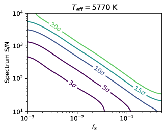
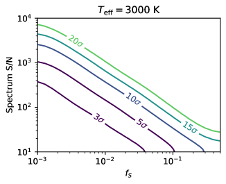
Figure 1: Signal-to-noise ratio of the cross-correlation function (colored contours) as a function of the signal-to-noise ratio of the simulated spectrum, and the spot coverage $f_{S}$ in the simulated spectrum, for a Sun-like star with $T_{\mbox{\scriptsize spot}}=3000$ K (upper) and for an M dwarf with $T_{\mbox{\scriptsize spot}}=2500$ K (lower). A typical, high-quality HARPS spectrum of a bright Sun-like star has $S/N\approx 300$, and Proxima Centauri typically has $S/N\approx 200$.

We plot the S/N curves for the observed CCF as a function of the spot coverage and each spectrum’s S/N in Figure 1. Each contour represents the signal-to-noise ratio of the peak in the the cross-correlation function for a given combination of the stellar spectral S/N and spot coverage $f_{S}$. The upper plot shows the results for a Sun-like star with $T_{\mbox{\scriptsize eff}}=5770$ K and $T_{\mbox{\scriptsize spot}}=3000$ K, and the lower plot represents an M star with $T_{\mbox{\scriptsize eff}}=3000$ K and $T_{\mbox{\scriptsize spot}}=2500$ K.

We focus first on the Sun-like case in the upper panel of Figure 1. Note that for a typical HARPS spectrum of a bright star with $S/N\sim 300$, and a Sun-like spot coverage $f_{S}<5\times 10^{-3}$, the CCF peak has $S/N<3$. In other words, Sun-like spot coverages on Sun-like stars should be undetectable with the cross-correlation function in individual exposures. If we imagine a bright Sun-like star with 10% spot coverage and HARPS spectra with $S/N\sim 300$, the CCF technique is expected to detect starspots at $10\sigma$ confidence.

The CCF signal is more significant as one inspects stars with smaller $T_{\mbox{\scriptsize eff}}$ and less extreme (warmer) spot temperatures. For the M dwarf in the lower panel of Figure 1, which has a similar effective temperature to Proxima Centauri and $T_{\mbox{\scriptsize spot}}=2500$ K, spots are more readily detectable via the CCF. Proxima Centauri is routinely observed by HARPS with $S/N\sim 200$, so watery spot coverages as small as $f_{S}=0.01$ could be detectable at $5\sigma$ if they were present.

4 Hunting for Spots

Figure 2: Identifying echelle orders with high-confidence detections of TiO in the stellar spectrum of Proxima Centauri, an M5V star, with a $T_{\mbox{\scriptsize eff}}=3000$ K (left) and $4000$ K (right). The background of each plot is shaded proportionately to the S/N ratio of the detection of TiO in that echelle order (dark is low signal, bright is high signal).

4.1 Testing the TiO line list

Figure 2 shows the CCF between an observed spectrum of Proxima Centauri (HARPS Program ID: 072.C-0488(E), PI: M. Mayor) and the TiO model spectra at 3000 K (left column, matching Proxima Centauri which has $T_{\mbox{\scriptsize eff}}\sim 3000$ K) and 4000 K (right column). Each panel represents one HARPS echelle order, with the central wavelength noted in the title. In black we plot the “weighted-mean absorption profile” CCF parameterization outlined in Section 3.1.

TiO is detected with $S/N>3$ in most echelle orders, peaking at $S/N\sim 22$ for the TiO template with the correct effective temperature. The order of magnitude variation in the $S/N$ for Proxima Centauri, which clearly has significant TiO absorption in every echelle order redward of 4500 Å (see Figure 8, in the Appendix), demonstrates that the line list is imperfect, in agreement with Hoeijmakers et al. (2015).

4.2 Search for cool spots on Proxima Centauri

In addition to using Proxima Centauri as a control target to identify the orders where the TiO line list is the most reliable, we can search for cool spots on Proxima Centauri. Proxima has $T_{\mbox{\scriptsize eff}}=2980\pm 80$ K (Ribas et al., 2017), so we assume dark star-spots may have temperatures of $\sim 2500$ K (Berdyugina, 2005), and search for emission from these spots using the cross-correlation function of the spectrum with a template for water at 2500 K. After all, water has even been detected in sunspots (Wallace et al., 1995).

Figure 3 shows that no significant detections of water absorption are present in any of the spectral orders red-ward of 6000 Å, where the water spectrum has small absorption features (see Figure 8). The lack of detectable spots could indicate that there are few cool spots, or their temperature contrast is significantly different from $\Delta T=500$ K, or the S/N of these spectra are insufficient to detect the relatively weak absorption lines from water.

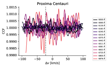
Figure 3: Null detection of water absorption in the high resolution spectrum of Proxima Centauri. For reference, the radial velocity of Proxima is $-22$ km s^-1, marked with the vertical dashed line.

4.3 Search for sunspots

The umbrae of sunspots reach temperatures as low as $\sim$4000 K (Solanki, 2003), and therefore we might expect a very spotted Sun to generate TiO absorption. Fortunately, there are also several Sun-observing spacecraft which have been imaging the Sun for decades, often simultaneously with HARPS observations of reflected sunlight via observations solar system targets, such as the Moon.

For several thousand publicly available lunar spectra from HARPS, we retrieve simultaneous Solar Dynamics Observatory (SDO) HMI continuum intensity imaging of the Sun. We find that the Sun was most spotted during lunar HARPS observations on UTC November 2, 2015 (Program ID: 096.C-0210(A), PI: P. Figueira), when two major spot groups were on the Earth-facing solar hemisphere – see Figure 4.

We cross correlate the solar spectrum with the 4000 K TiO template. We find no significant absorption in any of the nine observations which have $S/N>100$ on that night, in any of the four echelle orders where the TiO line list is expected to produce the strongest CCF signal based on the cross-correlation with the spectrum of Proxima Centauri.

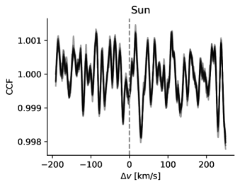
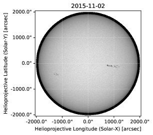
Figure 4: Left: cross-correlation functions of the 4000 K TiO template emission spectrum and two HARPS spectra of the Sun (reflected off of the Moon) on November 2, 2015 – a night with two large sunspot groups facing the Earth. The echelle order used in these plots is the one centered on 6797 Å, which is the order with the strongest CCF signal when cross-correlating the Proxima Centauri spectrum with the 3000 K TiO template. The vertical dashed line is the estimated radial velocity of the source. Right: SDO HMI continuum intensity image of the Sun during the HARPS observations, revealing the large sunspot groups which are not detected by the cross-correlation technique.

4.4 Search for starspots on 18 Sco

For more than 20 years, 18 Scorpii has been studied as a solar twin (Porto de Mello & da Silva, 1997), that is, a star with spectroscopic parameters exceptionally similar to the Sun’s (Cayrel de Strobel, 1996). Hall & Lockwood (2000) and Hall et al. (2007) showed that 18 Sco has a seven year activity cycle that is similar to the Sun’s in terms of total irradiance variation. Joint asteroseismic and spectroscopic analyses have yielded highly precise measurements of the stellar radius and mass (Bazot et al., 2011; Li et al., 2012; Bazot et al., 2012). Petit et al. (2008) used spectropolarimetry to show that its rotation period is $22.7\pm 0.5$ days, only a few days shorter than solar, and more recently Bazot et al. (2018) used asteroseismology to suggest that the age of 18 Sco may be consistent with solar (though estimates have varied from 0.3 Gyr to 5.8 Gyr, Tsantaki et al. 2013; Takeda et al. 2008; Mittag et al. 2016). Even under intense scrutiny, this star continues to appear remarkably similar to the Sun, so one might expect 18 Sco to have spots like the Sun does.

18 Sco has been the subject of various radial velocity searches for exoplanets with HARPS. We gather 4000 archival HARPS spectra of 18 Sco collected since 2006 under various observing programs. We stack all spectra of 18 Sco together by shifting the wavelength axis of each spectrum to maximize the cross-correlation with the previous spectrum. The coadded spectrum has $S/N\approx 2200$.

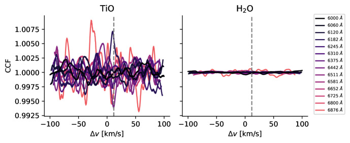
Figure 5: Cross-correlation function of 4000 stacked HARPS spectra of 18 Scorpii with the TiO ($T_{\mbox{\scriptsize spot}}=4000$ K) and water ($T_{\mbox{\scriptsize spot}}=2500$ K) templates, with a coadded $S/N\approx 2200$. The CCF produces no signal with either molecule, indicating a small spot coverage for 18 Sco. The vertical dashed line is the estimated radial velocity of the source.

The CCF of the stacked HARPS spectra and the TiO and water emission templates are shown in Figure 5. Each curve represents the CCF of a single echelle order with the template. If TiO or water absorption were present in the coadded spectrum, there would be a negative absorption feature dipping below unity near the radial velocity of the star ($v=11.90$ km s^-1), but no signal is detected.

In the case of the spectrum of 18 Sco, we have a Sun-like star with an unknown spot coverage and a coadded $S/N\approx 2200$. The null detection of water and TiO in the stacked spectrum of 18 Sco given the simulations in Section 3 places an upper limit on the spot covering fraction $f_{S}\lesssim 4\times 10^{-3}$. This is smaller than the Sun’s most extreme spot coverages near solar maximum, $f_{S}\approx 5\times 10^{-3}$ (Morris et al., 2017).

4.5 Search for the spots of HAT-P-11

HAT-P-11 is an active K4V dwarf in the Kepler field with a transiting hot Neptune. Transits revealed frequent starspot occultations (Deming et al., 2011; Sanchis-Ojeda & Winn, 2011), which yield approximate spot covering fractions $f_{S}=0.0-0.1$ (Morris et al., 2017). HAT-P-11 appears to have a $\sim$10 year activity cycle, and may be modestly more chromospherically active than planet hosts of similar rotation periods (Morris et al., 2018a). Recent ground-based photometry of spot occultations within the transit chord yielded spot coverage $f_{S}=0.14$ (Morris et al., 2018b). Morris et al. (2019) model the spectrum of HAT-P-11 as a linear combination of the spectra of HD 5857 and Gl 705, giving the spots $\Delta T_{\mathrm{eff}}=250$ K, similar to typical sunspot penumbra, finding a spot coverage consistent with previous measurements.

We cross-correlate 139 HARPS-N spectra of HAT-P-11 (Program ID: OPT15B_19, PI: D. Ehrenreich) with the TiO template at 4000 K in Figure 6. There is no significant absorption in the CCF due to TiO, despite HAT-P-11 being on average 100x more spotted than the Sun (Morris et al., 2017).

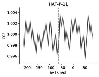
Figure 6: Cross-correlation functions of the HARPS-N spectra of the highly-spotted K4V star HAT-P-11 and the TiO template with $T_{\mbox{\scriptsize spot}}=4000$ K. The echelle order used in these plots is the one centered on 6722 Å, which is the order with the second strongest CCF signal when cross-correlating the Proxima Centauri spectrum with the 3000 K TiO template. The vertical dashed line is the radial velocity of the star.

4.6 Search for the cool regions of T Tauri Stars: LkCa 4 and AA Tau

LkCa 4 is a T Tauri star which is often classified as a K7 dwarf (Herbig et al., 1986). Gully-Santiago et al. (2017) used high-resolution near-infrared IGRINS spectra to show that the stellar surface of LkCa 4 is in fact dominated by cool regions, covering 80% of the stellar surface with $T_{\mathrm{cool}}\sim 2700-3000$ K. Hot regions make up the other 20% of the surface with $T_{\mathrm{hot}}\sim 4100$ K.

We examine the CCF of the LkCa 4 HARPS spectrum (Program ID: 074.C-0221(A), PI J. Bouvier) as a control to verify that TiO can be detected in stars earlier than M-type, when they are known to be extremely “spotted.” Figure 7 shows the CCF, confirming strong absorption features due to TiO near $T_{\mbox{\scriptsize spot}}=4000$ K. The clear CCF signal confirms that indeed the star has significant coverage by regions cooler than the K7 spectral type assigned to this star.

AA Tau is a K5 dwarf, and also a T Tauri star. We cross-correlate the HARPS spectrum of AA Tau (Program ID: 074.C-0221(A), PI J. Bouvier) with the TiO emission template at $T_{\mbox{\scriptsize spot}}=4000$ K. Again, we find evidence for significant absorption by TiO in the atmosphere of this “K” star, confirming that at least one other T Tauri star has significant coverage by cool regions, and that our CCF technique is performing as expected on a highly-spotted control star.

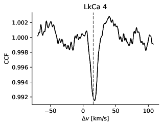
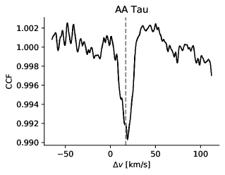
Figure 7: Cross-correlation functions of the HARPS spectra of the puzzling K7 dwarf LkCa 4 (left) and the K5 dwarf AA Tau (right), and the TiO template with $T_{\mbox{\scriptsize spot}}=4000$ K. The echelle order used in these plots is the one centered on 6800 Å, which is the order with the strongest CCF signal when cross-correlating the Proxima Centauri spectrum with the 3000 K TiO template. The vertical dashed line is the radial velocity of each star.

5 Conclusion

Starspots on Sun-like stars are functionally invisible in HARPS/HARPS-N spectra when using TiO as a tracer. While the invisibility of starspots to the CCF technique may dismay starspot hunters, exoplanet hunters searching for molecular absorption in exoplanet atmospheres can be confident that the signals they detect come from the exoplanet rather than the star. Starspots should be an insignificant source of TiO absorption in the spectra of exoplanetary systems with FGK host stars. Of course, one could also disentangle the stellar and planetary signals with to the difference in velocity between the star and the planet.

Appendix A Spectral Templates

Figure 8 shows the resulting TiO spectral templates each normalized by their maximum flux.

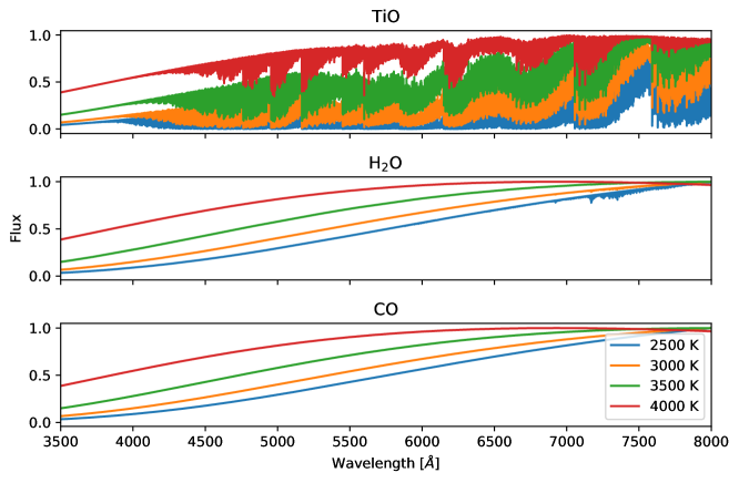
Figure 8: Spectral templates for TiO, H₂O, and CO at four temperatures. TiO shows significant absorption bands throughout the HARPS bandpass at all temperatures, while water only deviates significantly from a blackbody at $T<3000$ K. CO never deviates significantly from a blackbody in the temperature range and HARPS bandpass.

References

- Asplund et al. (2009) Asplund, M., Grevesse, N., Sauval, A. J., & Scott, P. 2009, ARA&A, 47, 481, doi: 10.1146/annurev.astro.46.060407.145222
- Astropy Collaboration et al. (2013) Astropy Collaboration, Robitaille, T. P., Tollerud, E. J., et al. 2013, A&A, 558, A33, doi: 10.1051/0004-6361/201322068
- Astropy Collaboration et al. (2018) Astropy Collaboration, Price-Whelan, A. M., Sipőcz, B. M., et al. 2018, ArXiv e-prints. https://arxiv.org/abs/1801.02634
- Barber et al. (2006) Barber, R. J., Tennyson, J., Harris, G. J., & Tolchenov, R. N. 2006, MNRAS, 368, 1087, doi: 10.1111/j.1365-2966.2006.10184.x
- Bazot et al. (2018) Bazot, M., Creevey, O., Christensen-Dalsgaard, J., & Meléndez, J. 2018, A&A, 619, A172, doi: 10.1051/0004-6361/201834058
- Bazot et al. (2011) Bazot, M., Ireland, M. J., Huber, D., et al. 2011, A&A, 526, L4, doi: 10.1051/0004-6361/201015679
- Bazot et al. (2012) Bazot, M., Campante, T. L., Chaplin, W. J., et al. 2012, A&A, 544, A106, doi: 10.1051/0004-6361/201117963
- Berdyugina (2005) Berdyugina, S. V. 2005, Living Reviews in Solar Physics, 2, 8, doi: 10.12942/lrsp-2005-8
- Bower et al. (2019) Bower, D. J., Kitzmann, D., Wolf, A. S., et al. 2019, A&A, 631, A103, doi: 10.1051/0004-6361/201935710
- Brogi et al. (2012) Brogi, M., Snellen, I. A. G., de Kok, R. J., et al. 2012, Nature, 486, 502, doi: 10.1038/nature11161
- Cayrel de Strobel (1996) Cayrel de Strobel, G. 1996, The Astronomy and Astrophysics Review, 7, 243, doi: 10.1007/s001590050006
- Deming et al. (2011) Deming, D., Sada, P. V., Jackson, B., et al. 2011, ApJ, 740, 33, doi: 10.1088/0004-637X/740/1/33
- Ducrot et al. (2018) Ducrot, E., Sestovic, M., Morris, B. M., et al. 2018, AJ, 156, 218, doi: 10.3847/1538-3881/aade94
- Gully-Santiago et al. (2017) Gully-Santiago, M. A., Herczeg, G. J., Czekala, I., et al. 2017, ApJ, 836, 200, doi: 10.3847/1538-4357/836/2/200
- Hall et al. (2007) Hall, J. C., Henry, G. W., & Lockwood, G. W. 2007, AJ, 133, 2206, doi: 10.1086/513195
- Hall & Lockwood (2000) Hall, J. C., & Lockwood, G. W. 2000, ApJ, 545, L43, doi: 10.1086/317331
- Hamre et al. (2013) Hamre, B., Stamnes, S., Stamnes, K., & Stamnes, J. J. 2013, in American Institute of Physics Conference Series, Vol. 1531, American Institute of Physics Conference Series, 923–926, doi: 10.1063/1.4804922
- Hauschildt & Baron (1999) Hauschildt, P. H., & Baron, E. 1999, Journal of Computational and Applied Mathematics, 109, 41
- Herbig et al. (1986) Herbig, G. H., Vrba, F. J., & Rydgren, A. E. 1986, AJ, 91, 575, doi: 10.1086/114039
- Hoeijmakers et al. (2015) Hoeijmakers, H. J., de Kok, R. J., Snellen, I. A. G., et al. 2015, A&A, 575, A20, doi: 10.1051/0004-6361/201424794
- Hunter (2007) Hunter, J. D. 2007, Computing in Science and Engineering, 9, 90, doi: 10.1109/MCSE.2007.55
- Husser et al. (2013) Husser, T.-O., Wende-von Berg, S., Dreizler, S., et al. 2013, A&A, 553, A6, doi: 10.1051/0004-6361/201219058
- John (1988) John, T. L. 1988, A&A, 193, 189
- Jones et al. (2001) Jones, E., Oliphant, T., Peterson, P., et al. 2001, SciPy: Open source scientific tools for Python. http://www.scipy.org/
- Karman et al. (2019) Karman, T., Gordon, I. E., van der Avoird, A., et al. 2019, Icarus, 328, 160, doi: 10.1016/j.icarus.2019.02.034
- Li et al. (2012) Li, T. D., Bi, S. L., Liu, K., Tian, Z. J., & Shuai, G. Z. 2012, A&A, 546, A83, doi: 10.1051/0004-6361/201219063
- Mayor et al. (2003) Mayor, M., Pepe, F., Queloz, D., et al. 2003, The Messenger, 114, 20
- McKemmish et al. (2019) McKemmish, L. K., Masseron, T., Hoeijmakers, H. J., et al. 2019, MNRAS, 488, 2836, doi: 10.1093/mnras/stz1818
- Mittag et al. (2016) Mittag, M., Schröder, K.-P., Hempelmann, A., González-Pérez, J. N., & Schmitt, J. H. M. M. 2016, A&A, 591, A89, doi: 10.1051/0004-6361/201527542
- Morris et al. (2018a) Morris, B. M., Agol, E., Davenport, J., & Hawley, S. 2018a, MNRAS
- Morris et al. (2019) Morris, B. M., Curtis, J. L., Sakari, C., Hawley, S. L., & Agol, E. 2019, arXiv e-prints, arXiv:1907.00423. https://arxiv.org/abs/1907.00423
- Morris et al. (2018b) Morris, B. M., Hawley, S. L., & Hebb, L. 2018b, Research Notes of the American Astronomical Society, 2, 26, doi: 10.3847/2515-5172/aaac2e
- Morris et al. (2017) Morris, B. M., Hebb, L., Davenport, J. R. A., Rohn, G., & Hawley, S. L. 2017, ApJ, 846, 99, doi: 10.3847/1538-4357/aa8555
- Morris et al. (2018c) Morris, B. M., Agol, E., Hebb, L., et al. 2018c, ApJ, 863, L32, doi: 10.3847/2041-8213/aad8aa
- Neff et al. (1995) Neff, J. E., O’Neal, D., & Saar, S. H. 1995, ApJ, 452, 879, doi: 10.1086/176356
- O’Neal et al. (1998) O’Neal, D., Neff, J. E., & Saar, S. H. 1998, ApJ, 507, 919, doi: 10.1086/306340
- O’Neal et al. (2004) O’Neal, D., Neff, J. E., Saar, S. H., & Cuntz, M. 2004, AJ, 128, 1802, doi: 10.1086/423438
- O’Neal et al. (2001) O’Neal, D., Neff, J. E., Saar, S. H., & Mines, J. K. 2001, AJ, 122, 1954, doi: 10.1086/323093
- O’Neal et al. (1996) O’Neal, D., Saar, S. H., & Neff, J. E. 1996, ApJ, 463, 766, doi: 10.1086/177288
- Pérez & Granger (2007) Pérez, F., & Granger, B. E. 2007, Computing in Science and Engineering, 9, 21, doi: 10.1109/MCSE.2007.53
- Petit et al. (2008) Petit, P., Dintrans, B., Solanki, S. K., et al. 2008, MNRAS, 388, 80, doi: 10.1111/j.1365-2966.2008.13411.x
- Porto de Mello & da Silva (1997) Porto de Mello, G. F., & da Silva, L. 1997, ApJ, 482, L89, doi: 10.1086/310693
- Rackham et al. (2018) Rackham, B. V., Apai, D., & Giampapa, M. S. 2018, ApJ, 853, 122, doi: 10.3847/1538-4357/aaa08c
- Ramsey & Nations (1980) Ramsey, L. W., & Nations, H. L. 1980, ApJ, 239, L121, doi: 10.1086/183306
- Ribas et al. (2017) Ribas, I., Gregg, M. D., Boyajian, T. S., & Bolmont, E. 2017, A&A, 603, A58, doi: 10.1051/0004-6361/201730582
- Sanchis-Ojeda & Winn (2011) Sanchis-Ojeda, R., & Winn, J. N. 2011, ApJ, 743, 61, doi: 10.1088/0004-637X/743/1/61
- Snellen et al. (2010) Snellen, I. A. G., de Kok, R. J., de Mooij, E. J. W., & Albrecht, S. 2010, Nature, 465, 1049, doi: 10.1038/nature09111
- Solanki (2003) Solanki, S. K. 2003, A&A Rev., 11, 153, doi: 10.1007/s00159-003-0018-4
- Stock et al. (2018) Stock, J. W., Kitzmann, D., Patzer, A. B. C., & Sedlmayr, E. 2018, MNRAS, 479, 865, doi: 10.1093/mnras/sty1531
- SunPy Community et al. (2015) SunPy Community, T., Mumford, S. J., Christe, S., et al. 2015, Computational Science and Discovery, 8, 014009, doi: 10.1088/1749-4699/8/1/014009
- Takeda et al. (2008) Takeda, G., Ford, E. B., Sills, A., et al. 2008, VizieR Online Data Catalog, 216
- Tsantaki et al. (2013) Tsantaki, M., Sousa, S. G., Adibekyan, V. Z., et al. 2013, A&A, 555, A150, doi: 10.1051/0004-6361/201321103
- Van Der Walt et al. (2011) Van Der Walt, S., Colbert, S. C., & Varoquaux, G. 2011, ArXiv e-prints. https://arxiv.org/abs/1102.1523
- Vogt (1979) Vogt, S. S. 1979, PASP, 91, 616, doi: 10.1086/130549
- Wakeford et al. (2019) Wakeford, H. R., Lewis, N. K., Fowler, J., et al. 2019, AJ, 157, 11, doi: 10.3847/1538-3881/aaf04d
- Wallace et al. (1995) Wallace, L., Bernath, P., Livingston, W., et al. 1995, Science, 268, 1155. http://www.jstor.org/stable/2888375