Inference for a test-negative case-control study with added controls

Abstract

Test-negative designs with added controls have recently been proposed to study COVID-19. An individual is test-positive or test-negative accordingly if they took a test for a disease but tested positive or tested negative. Adding a control group to a comparison of test-positives vs test-negatives is useful since additional comparison of test-positives vs controls can have potential biases different from the first comparison. Bonferroni correction ensures necessary type-I error control for these two comparisons done simultaneously. We propose two new methods for inference which have better interpretability and higher statistical power for these designs. These methods add a third comparison that is essentially independent of the first comparison, but our proposed second method often pays much less for these three comparisons than what a Bonferroni correction would pay for the two comparisons.

Running Head: Test-negative case-control study with added controls.

Keywords: Case-control studies; closed testing; multi-step procedure; test-negative designs.

Conflict of interest statement: There is no conflict of interest.

Source of funding: None.

Data and code availability: We provide computing code in the supplementary materials.

keywords: Case-control studies; Closed testing; Confidence intervals; Potential biases; Second control group.

Test-negative studies compare exposures in cases who take a test for a particular disease and test positive vs. controls who also take the test but test negative.⁵; ⁷ A test-negative study with added controls (TNSWAC) supplements with controls who did not take the test. TSNWACs have been used to study antibiotic resistance⁴ and proposed to study COVID-19.⁸ The standard inference approach has been to present two exposure rate comparisons,

• test-positives to test-negatives

• test-positives to controls

To control the familywise Type I error rate for multiple comparisons at level $\alpha$ (e.g., $\alpha=0.05$), the Bonferroni inequality can be used and each comparison done at level $\alpha/2$. Here we propose different inference strategies that can provide greater interpretability and power.

A valuable feature of TSNWACs is that comparisons (i) and (ii) may have different potential biases.⁸ Evidence is strengthened when diverse approaches with diverse potential biases produce similar results.⁶; ³ However, comparisons (i) and (ii) are dependent – see Figure 1A – and might tend to agree just because of this dependence. It is important to distinguish new evidence from the same evidence repeated twice.³ To this end, it is useful to supplement comparisons (i)-(ii) with comparison (iii) test-positives pooled with test-negatives to controls, which is essentially independent of (i) – see Figure 1B and supplement – and may suffer from different potential biases than (i).¹ For example, it has been hypothesized that smoking protects against Covid-19.² Comparison (i) may be biased because test-negatives may have some other infection (e.g., the flu) for which smoking increases risk and comparisons (ii) and (iii) may be biased because test-takers tend to be “health seeking.”⁷ Finding evidence of smoking being protective in all comparisons (i)-(iii) would strengthen evidence compared to just comparisons (i)-(ii) in part because the latter comparisons are dependent.

The following are two procedures that consider comparisons (i)-(iii) and control the familywise error rate for multiple comparisons at $\alpha$ (proof/code in supplement). The first procedure is (1) test the null hypothesis of no exposure effect in comparison (i), $H_{0(i)}$, at level $\alpha/2$ (i.e., reject if $p$-value $\leq\alpha_{2}$) and test the null of no exposure effect in comparison (ii), $H_{0(ii)}$, at level $\alpha/2$ and (2) if and only if both nulls are rejected, test the null of no exposure effect in comparison (iii), $H_{0(iii)}$, at level $\alpha$. The second procedure is

• Test $H_{0(ii)}$ at level $\alpha/2$. If $H_{0(ii)}$ is rejected, set $\lambda=\alpha$; otherwise, $\lambda=\alpha/2$.

• Test the null of no exposure effect in either comparison (i) and/or comparison (iii), $H_{0(i)}\cup H_{0(iii)}$, at level $\lambda$. This could be done by Fisher’s combination method since comparisons (i) and (iii) are essentially independent under the null.¹ If the null $H_{0(i)}\cup H_{0(iii)}$ is not rejected, stop testing.

• If $H_{0(i)}\cup H_{0(iii)}$ was rejected in (2), then test $H_{0(i)}$ and $H_{0(iii)}$ each at level $\lambda$.

• If $\lambda=\alpha/2$ and both $H_{0(i)}$ and $H_{0(iii)}$ were rejected in (3), then test $H_{0(ii)}$ at level $\alpha$ and reject if $p$-value $\leq\alpha$.

For example, suppose the p-values for $H_{0(i)}$, $H_{0(ii)}$ and $H_{0(iii)}$ were .04, .03 and .04 respectively, then the standard procedure would not reject any null hypotheses whereas the second procedure would reject all nulls (note: $p$-value for $H_{0(i)}\cup H_{0(iii)}$ using Fisher’s combination test is .012). Confidence intervals for magnitudes of effect can be formed using both procedures, see supplement. Figure 1C compares the power of the two proposed procedures and the standard procedure in a simulation. Both proposed procedures increase power over the standard procedure in the simulated setting with the second procedure providing more power.

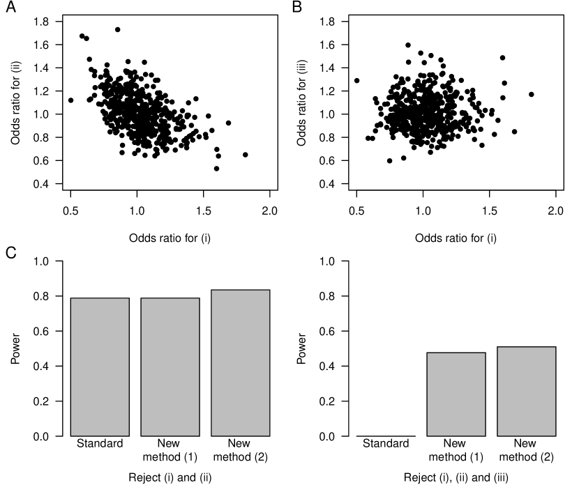
Figure 1: Simulated results on inference for TNSWAC. In panels A and B the null hypothesis is true and there is no difference in the exposure between the test-positives, test-negatives and controls. In panel A analyses (i) and (ii) show dependence and in panel B analyses (i) and (iii) show approximate uncorrelatedness. Two plots in Panel C show the simulated powers of three different methods of analyses of TNSWAC, calculated from 10,000 simulated instances. One simulated study consists of 1,250 individuals of, on average, 40% controls, 30% test-negatives and 30% test-positives. Under the null, in Panel A and B, the frequency of an exposure is constant 20% in each of these three groups. In panel C, the odds ratio of an exposure is 1.75 for test-positives versus controls and the odds ratio of an exposure is 1.75 for test-positives versus test-negatives. R code for the simulation is provided in the supplement.

Bikram Karmakar and Dylan Small
University of Florida and University of Pennsylvania

1 Familywise error rate control

Setup: Consider the following three null hypotheses: $H_{0(i)}$, no difference in exposure between test-positives and test-negatives; $H_{0(ii)}$, no difference in exposure between test-positives and controls; and $H_{0(iii)}$, no difference in the test-positives or test-negatives and controls. In the following $P_{(i)}$, $P_{(ii)}$ and $P_{(iii)}$ correspond to the three p-values calculated for these hypotheses from the corresponding comparisons.

In this setup a method provides a level $\alpha$ familywise error rate control if the probability of rejecting any true null hypothesis among the three null hypotheses is at most $\alpha$. In the following we let $\mathcal{R}_{S}$ denote the event that at least one of the nulls are rejected among $\{H_{0s}:s\in S\}$ where $S\subseteq\{(i),(ii),(iii)\}$. We show here that familywise error rate is controlled for both Method 1 and Method 2.

Method 1. Note first that $H_{0(iii)}$ is false when and only when one of $H_{0(i)}$ or $H_{0(ii)}$ were false.

Since Method 1 can reject $H_{0(iii)}$ in step (2) only when both $H_{0(i)}$ and $H_{0(ii)}$ are rejected at step (1), we have $\mathcal{R}_{(iii)}\subseteq\mathcal{R}_{(i)}\cap\mathcal{R}_{(ii)}$, hence $\mathcal{R}_{(i),(ii),(iii)}\subseteq\mathcal{R}_{(i),(ii)}$.

To show familywise error rate control, consider now the different possibilities of the three hypotheses being true or false separately.

(a)  When all three hypotheses are true, the familywise error rate is

$$\text{pr}(\mathcal{R}_{(i),(ii),(iii)}) \leq\text{pr}(\mathcal{R}_{(i),(ii)})$$

$$\leq\text{pr}(\mathcal{R}_{(i)})+\text{pr}(\mathcal{R}_{(ii)})$$

$$=\text{pr}(P_{(i)}\leq\alpha/2)+\text{pr}(P_{(ii)}\leq\alpha/2)$$

$$\leq\alpha/2+\alpha/2=\alpha.$$

(b)  When $H_{0(i)}$ is true but $H_{0(ii)}$ is false, hence $H_{0(iii)}$ is false, the familywise error rate is

$$\text{pr}(\mathcal{R}_{(i)})=\text{pr}(P_{(i)}\leq\alpha/2)\leq\alpha/2\leq\alpha.$$

(c)  Finally, when $H_{0(ii)}$ is true but $H_{0(i)}$ is false, hence $H_{0(iii)}$ is false, the familywise error rate is

$$\text{pr}(\mathcal{R}_{(ii)})=\text{pr}(P_{(ii)}\leq\alpha/2)\leq\alpha/2\leq\alpha.$$

Hence, the familywise error rate is always controlled.

Method 2.  First we expand the notation $\mathcal{R}_{S}$ to denote the event that at least one of the nulls are rejected among $\{H_{0s}:s\in S\}$ where $S\subseteq\{(i),(ii),(iii),(i)\wedge(ii)\}$, where $H_{0(i)\wedge(iii)}=H_{0(i)}\cap H_{0(iii)}$. Thus, $H_{0(i)\wedge(iii)}$ is false is the same as at least one $H_{0(i)}$ $H_{0(iii)}$ is false, and only when both $H_{0(i)}$ and $H_{0(iii)}$ are true we will have $H_{0(i)\wedge(iii)}$ true.

Now we use the result that $P_{(i)}$ and $P_{(iii)}$ are essentially independent and $P_{(i)\wedge(iii)}$, Fisher’s combination of these two p-values, is a valid p-value under $H_{0(i)\wedge(iii)}$.¹ (see footnote)

Consider again the different combinations of the three hypotheses being true or false. We can reduce some effort in this enumeration by noting that $H_{0(iii)}$ is false when and only when one of $H_{0(i)}$ or $H_{0(ii)}$ were false.

(a)  When all three of $H_{0(i)}$, $H_{0(ii)}$ and $H_{0(iii)}$ are true, the familywise error rate is

$$\text{pr}(\mathcal{R}_{(i),(ii),(iii)}) \leq\text{pr}(\mathcal{R}_{(ii)}\text{ at level }\alpha/2\text{ in step (1) or }\mathcal{R}_{(i)\wedge(iii)}\text{ at level }\alpha/2\text{ in step (2)})$$

$$\leq\text{pr}(\mathcal{R}_{(ii)}\text{ at level }\alpha/2)+\text{pr}(\mathcal{R}_{(i)\wedge(iii)}\text{ at level }\alpha/2)$$

$$=\text{pr}(P_{(ii)}\leq\alpha/2)+\text{pr}(P_{(i)\wedge(iii)}\leq\alpha/2)$$

$$\leq\alpha/2+\alpha/2=\alpha.$$

(b)  When $H_{0(i)}$ is true but $H_{0(ii)}$ is false, hence $H_{0(iii)}$ is false, the familywise error rate is

$$\text{pr}(\mathcal{R}_{(i)}) =\text{pr}(\mathcal{R}_{(i)}\text{ at level }\alpha/2\text{ or at level }\alpha\text{ in step (3), by whether $\lambda=\alpha/2$ or $=\alpha$})$$

$$\leq\text{pr}(\mathcal{R}_{(i)}\text{ at level }\alpha)$$

$$=\text{pr}(P_{(i)}\leq\alpha)\leq\alpha.$$

(c)  Finally, when $H_{0(ii)}$ is true but $H_{0(i)}$ is false, hence $H_{0(iii)}$ is false, the familywise error rate is

$$\text{pr}(\mathcal{R}_{(ii)}) =\text{pr}(\mathcal{R}_{(ii)}\text{ at level }\alpha/2\text{ or at level }\alpha\text{ in step (3), by whether $\lambda=\alpha/2$ or $=\alpha$})$$

$$\leq\text{pr}(\mathcal{R}_{(ii)}\text{ at level }\alpha)$$

$$=\text{pr}(P_{(ii)}\leq\alpha)\leq\alpha.$$

Hence, the familywise error rate is always controlled.

2 Confidence sets for the magnitude of effects

Notation:  We can create confidence sets for the effects of the exposure using the methods discussed in the letter. Some new notation are needed. In the following a subscript $P$ is for test-positives, $N$ for test-negatives, and $C$ for the added controls. Also, $n$ with appropriate subscript denotes the counts of a particular group of individuals. For example, $n_{P1}$ denotes the number of exposed test-positives and $n_{C0}$ the number of unexposed test-negatives, and $n_{PN1}$ is the number of exposed test-positives or test-negatives.

Data tables:  The collected data can be tabulated in three tables corresponding to the three comparisons (i), (ii) and (iii).

Comparison (i) Exposed Unexposed Test-positive $n_{P1}$ $n_{P0}$ Test-negative $n_{N1}$ $n_{N0}$ Total $n_{PN1}$ $n_{PN0}$        Comparison (ii) Exposed Unexposed Test-positive $n_{P1}$ $n_{P0}$ Control $n_{C1}$ $n_{C0}$ Total $n_{PC1}$ $n_{PC0}$

Comparison (iii) Exposed Unexposed Test-positive or negative $n_{PN1}$ $n_{PN0}$ Control $n_{C1}$ $n_{C0}$ Total $n_{PNC1}$ $n_{PNC0}$

A p-value for a given one of the three comparisons can be calculated from the corresponding table, e.g., using Fisher’s exact test. For example, $P_{(ii)}$ is the p-value calculated from the 2-by-2 table above with the numbers $n_{P1},n_{C1},n_{P0}$ and $n_{C0}$.

Effects of interest:  We have three effects of interest for the exposure, between test-positives and test-negatives, between test-positives and controls, and one between test-negatives and controls. We denote these effects as $\theta_{P,N},\theta_{P,C}$ and $\theta_{N,C}$, which are defined below. These are called attributable effects.

The effect $\theta_{P,N}$ is the ratio of the number of individuals who became test-positive because of the exposure, but in the absence of it would have been test-negative minus the number of individuals who became test-negative because of the exposure but in the absence of it would have been test-positive, divided by the number of exposed test-positives or test-negatives. Notice that $\theta_{P,N}$ is a number between -1 and 1; $\theta_{P,N}=0$ if exposure did not move anyone from being test-positive compared to test-negative without exposure or the reverse. If $\theta_{P,N}$ is positive, there individuals for whom the exposure caused them to become test-positive. Similarly, if $\theta_{P,N}$ is negative, there are individuals for whom the exposure caused them to become test-negative. In summary, $\theta_{P,N}$is the net effect of the exposure on becoming test-positive over test-negative for exposed tested individuals.

The second effect $\theta_{P,C}$ is defined similarly. By our definition, $\theta_{P,C}$ is the net effect of the exposure for test-positives versus controls relative to all exposed individuals either test-positive or control. We have $\theta_{P,C}=0$ if the exposure did not make any change in who became test-positive over control or the reverse.

Finally, we define a third attributable effect $\theta_{N,C}$ in the same way to denote the net effect of the exposure on becoming test-negative over control for all exposed non test-positive individuals.

A method that calculates p-values using the three tables above is testing the hypothesis of no effect of the exposure that $\theta_{P,N}=0,\theta_{P,C}=0$ and $\theta_{N,C}=0$.

Confidence sets:  We construct confidence sets for the effects $\theta_{P,N},\theta_{P,C}$ and $\theta_{N,C}$. To do this we have to explain how to test that $\theta_{P,N}=\theta_{P,N}^{{}^{\star}},\theta_{P,C}=\theta_{P,C}^{{}^{\star}}$ and $\theta_{N,C}=\theta_{N,C}^{{}^{\star}}$ where $\theta_{P,N}^{{}^{\star}},\theta_{P,C}^{{}^{\star}}$ and $\theta_{N,C}^{{}^{\star}}$ could be different from 0, not no effect of the exposure. When they are different from 0, we adjust the observed tables based on these effects to create tables of the potential outcomes under no exposure.

Adjusted comparison (i) Exposed Unexposed Test-positive $n_{P1}-\theta_{P,N}^{{}^{\star}}n_{PN1}-\theta_{P,C}^{{}^{\star}}n_{PC1}$ $n_{P0}$ Test-negative $n_{N1}+\theta_{P,N}^{{}^{\star}}n_{PN1}-\theta_{N,C}^{{}^{\star}}n_{NC1}$ $n_{N0}$

Adjusted comparison (ii) Exposed Unexposed Test-positive $n_{P1}-\theta_{P,N}^{{}^{\star}}n_{PN1}-\theta_{P,C}^{{}^{\star}}n_{PC1}$ $n_{P0}$ Control $n_{C1}+\theta_{P,C}^{{}^{\star}}n_{PC1}+\theta_{N,C}^{{}^{\star}}n_{NC1}$ $n_{C0}$

Adjusted comparison (iii) Exposed Unexposed Test-positive or negative $n_{PN1}-\theta_{P,C}^{{}^{\star}}n_{PC1}-\theta_{N,C}^{{}^{\star}}n_{NC1}$ $n_{PN0}$ Control $n_{C1}+\theta_{P,C}^{{}^{\star}}n_{PC1}+\theta_{N,C}^{{}^{\star}}n_{NC1}$ $n_{C0}$

Using either Method 1 or Method 2 we could test these three tables at level $\alpha$. Either method will make decisions to reject or not reject these adjusted tables. Then we write ${R}_{(i)}(\theta_{P,N}^{{}^{\star}},\theta_{P,C}^{{}^{\star}},\theta_{N,C}^{{}^{\star}}),$ ${R}_{(ii)}(\theta_{P,N}^{{}^{\star}},\theta_{P,C}^{{}^{\star}},\theta_{N,C}^{{}^{\star}})$ and ${R}_{(iii)}(\theta_{P,N}^{{}^{\star}},\theta_{P,C}^{{}^{\star}},\theta_{N,C}^{{}^{\star}})$ as binary variables which are 1 or 0 according to whether comparison (i), (ii) or (iii) is rejected, respectively, based on these adjusted tables. Our confidence interval is

$$\Big{\{}(\theta_{P,N}^{{}^{\star}},\theta_{P,C}^{{}^{\star}},\theta_{N,C}^{{}^{\star}}):\prod_{s\in\{(i),(ii),(iii)\}}{R}_{s}(\theta_{P,N}^{{}^{\star}},\theta_{P,C}^{{}^{\star}},\theta_{N,C}^{{}^{\star}})=0\Big{\}}.$$

Since either method performed at level $\alpha$ provides familywise error rate control at $\alpha$, this confidence interval will have a minimal coverage of $1-\alpha$ for both Method 1 and Method 2.

3 R code to implement new method (2)

Let p_i, p_ii and p_iii be variables in R that record the p-values from the three comparisons. They can be calculated using the syntax p_i = fisher.test(e_i, g_i)$p where e_i is a variable recording of exposure status, and g_i is a variable recording the case status only for the test-positives and test-negatives. e_ii, g_ii and e_iii, g_iii have the same role in the following code corresponding to the comparisons (i) and (iii) respectively.

## Significance level for familywise error rate control
alpha <- 0.05
alpha.2 <- alpha/2

## p-values computed from the three comparisons
p_i = fisher.test(e_i, g_i)$p
p_ii = fisher.test(e_ii, g_ii)$p
p_iii = fisher.test(e_iii, g_iii)$p

### Start of Method 2Ψ###
r_i = r_ii = r_iii = 0 ΨΨ# an inference for reject, value 1, or 0.
## Step (1)
r_ii = 1*(p_ii < alpha.2)
lambda = ifelse(r_ii, alpha, alpha-alpha.2)
## Step (2)
# Fisher’s combination
p_i_or_iii = pchisq(-2*log(p_i*p_iii), 4, lower.tail=FALSE)
r_i_or_iii = 1*(p_i_or_iii < lambda)
## Step (3)
if(r_i_or_iii)
     r_i = 1*(r_i < lambda);    r_iii = 1*(r_iii < lambda)
## Step (4)Ψ
if(r_i & r_iii)  r_ii = 1*(p_ii < alpha)
### Final inference
c(r_i, r_ii, r_iii)
#### END OF CODE ####

References

- Karmakar et al. 2020 Bikram Karmakar, Chyke A Doubeni, and Dylan S Small. Evidence factors in a case-control study with application to the effect of flexible sigmoidoscopy screening on colorectal cancer. Annals of Applied Statistics, forthcoming, 2020.
- Miyara et al. 2020 Makoto Miyara, Florence Tubach, and Zahir Amoura. Low incidence of daily active tobacco smoking in patients with symptomatic covid-19 infection. Preprint, 04 2020. doi: 10.32388/WPP19W.
- Rosenbaum 2010 Paul R Rosenbaum. Evidence factors in observational studies. Biometrika, 97(2):333–345, 2010.
- Søgaard et al. 2017 Mette Søgaard, Uffe Heide-Jørgensen, Jan P Vandenbroucke, Henrik C Schønheyder, and CMJE Vandenbroucke-Grauls. Risk factors for extended-spectrum -lactamase-producing escherichia coli urinary tract infection in the community in denmark: a case–control study. Clinical Microbiology and Infection, 23(12):952–960, 2017.
- Sullivan et al. 2016 Sheena G Sullivan, Eric J Tchetgen Tchetgen, and Benjamin J Cowling. Theoretical basis of the test-negative study design for assessment of influenza vaccine effectiveness, 2016.
- Susser 1973 Mervyn Susser. Causal thinking in the health sciences: concepts and strategies of epidemiology. In Causal thinking in the health sciences: concepts and strategies of epidemiology. 1973.
- Vandenbroucke and Pearce 2019 Jan P Vandenbroucke and Neil Pearce. Test-negative designs: Differences and commonalities with other case–control studies with “other patient” controls. Epidemiology, 30(6):838–844, 2019.
- Vandenbroucke et al. 2020 Jan P Vandenbroucke, Elizabeth B Brickley, Christina MJE Vandenbroucke-Grauls, and Neil Pearce. Analysis proposals for test-negative design and matched case-control studies during widespread testing of symptomatic persons for sars-cov-2. arXiv preprint arXiv:2004.06033, 2020.
Supplement to “Inference for a test-negative case-control study with added controls”