Electric-Field-Induced Instabilities
in Nematic Liquid Crystals

Abstract

Systems involving nematic liquid crystals subjected to magnetic fields or electric fields are modeled using the Oseen-Frank macroscopic continuum theory, and general criteria are developed to assess the local stability of equilibrium solutions. The criteria take into account the inhomogeneity of the electric field (assumed to arise from electrodes held at constant potential) and the mutual influence of the electric field and the liquid-crystal director field on each other. The criteria show that formulas for the instability thresholds of electric-field Fréedericksz transitions cannot in all cases be obtained from those for the analogous magnetic-field transitions by simply replacing the magnetic parameters by the corresponding electric parameters, contrary to claims in standard references. This finding is consistent with observations made in [Arakelyan, Karayan, Chilingaryan, Sov. Phys. Dokl., 29 (1984), pp. 202–204]. A simple analytical test is provided to determine when an electric-field-induced instability can differ qualitatively from the analogous magnetic-field-induced instability; the test depends only on the orientations of the ground-state fields and their admissible variations. For the systems we study, it is found that taking into account the full coupling between the electric field and the director field can either elevate or leave unchanged an instability threshold (never lower it), compared to the threshold provided by the magnetic-field analogy (i.e., compared to treating the electric field as a uniform external force field). The physical mechanism that underlies the effect of elevating an instability threshold is the added free energy associated with a first-order change in the ground-state electric field caused by a perturbation of the ground-state director field. Examples are given that involve classical Fréedericksz transitions and also periodic instabilities, with the periodic instability of Lonberg and Meyer [Phys. Rev. Lett., 55 (1985), pp. 718–721] being further explored. The inclusion of flexoelectric terms in the theory is studied, and it is found that these terms are not capable of altering the instability thresholds of any of the classical Fréedericksz transitions, consistent with known results for the cases of the magnetic-field and the electric-field splay transitions.

49K20, 49K35, 49K40, 49S05, 78A30

1 Introduction

Our interest is in macroscopic continuum models for the orientational properties of materials in a liquid crystal phase, a complex partially ordered fluid phase exhibited by certain materials in certain parameter ranges. Such models are used at the scales of typical devices and experiments involving these kinds of materials (micrometer-scale thin films, and the like). Liquid crystals are very responsive to external stimuli, such as magnetic fields and electric fields, and this has been one of the keys to their usefulness in technological applications. This response frequently manifests itself in an instability such that an abrupt change in the orientational properties of the material occurs at a critical threshold of the strength of the applied magnetic or electric field, the textbook examples of this being “Fréedericksz transitions”—see [9, §3.2.3] or [38, §3.4] or [39, §4.2]. Our main objective is to illuminate differences between instabilities induced by magnetic fields versus those induced by electric fields. We do this via the development of stability criteria that take into account the inhomogeneity of the electric field and its coupling to the orientational properties of the material. The characterizations of local stability that we develop mimic familiar results found in equality-constrained optimization theory in $\mathbb{R}^{n}$.

At the macroscopic level of modeling, the orientational state of a material in a uniaxial nematic liquid crystal phase is characterized by a unit-length vector field $\bm{n}$ (the “director field”), which represents the average orientation of the distinguished axis of the anisometric molecules in a fluid element at a point. Central to the modeling of equilibrium configurations of the director field is an appropriate expression for the free energy of the system, a thermodynamic potential that serves as a work function for isothermal, reversible processes. In the models of interest to us, the material is assumed to be incompressible. For simplicity, we restrict our attention to achiral uniaxial nematic liquid crystals (the simplest liquid crystal phase). Such materials are characterized by intermolecular forces that encourage parallel alignment of directors, leading to uniform ground-state director fields. Other influences (boundary conditions, external force fields) can effect nonuniform equilibrium configurations of $\bm{n}$, at a cost of distortional elastic energy. Details are presented in what follows. Standard references include [9, 38, 39].

The force fields of external origin most commonly encountered in the context of liquid crystals are magnetic fields and electric fields. Magnetic fields are influenced by a liquid crystal medium, which is anisotropic with magnetic susceptibilities that depend on the orientational state of the material at a point. For the parameter values of typical liquid crystal materials, however, this influence is negligible [2], [17, §2.1]. Thus, a magnetic field in a liquid crystal can be treated as a uniform external field. An electric field is influenced by the state of the liquid crystal material in a similar fashion; however, the coupling is much stronger and should not be ignored [2], [17, §2.1]. Thus, the equilibrium state of a liquid crystal subjected to an electric field should be determined in a self-consistent way, with the director field and the electric field treated as coupled state variables. This coupling in general leads to inhomogeneities of the electric field and complicates the determination of equilibrium fields and the assessment of their local stability properties.

While the differences between magnetic fields and electric fields in liquid crystals have been appreciated for some time, the widely held view is that they give rise to only modest quantitative differences but not to qualitative differences in the context of instabilities such as Fréedericksz transitions. For example, in [9, §3.3.1] (referencing [21]) and [38, §3.5], it is asserted that electric-field Fréedericksz thresholds can be obtained from the formulas for magnetic-field thresholds by simply substituting the electric parameters for the corresponding magnetic parameters. In fact, this was borne out in [10], where the electric-field Fréedericksz transition in a particular geometry was analyzed taking into account the full coupling between the director field and the electric field. There it was found that in contrast to the approximation by a uniform electric field, slightly smaller values were obtained for the distortion of the liquid crystal director field past the onset of the instability, though the critical threshold of the electric field itself was the same in the coupled case as in the case of the approximation by a uniform external electric field (consistent with the recipe of [9, §3.3.1] and [38, §3.5]). The analysis of [10] is recounted in [38, §3.5].

A common use of the threshold formulas for the various Fréedericksz transitions is in determining via experimental measurements certain material-dependent parameters of different liquid crystals [9, §3.2.3.1]. Such experiments can be done with magnetic fields or with electric fields, whichever is more convenient, and experimentalists invariably take for granted the validity of the simple relationships between the formulas for the magnetic-field threshold versus the electric-field threshold implied by the recipes of [9, §3.3.1] and [38, §3.5]—see, for example, [4] or [12, Ch. 5] for more discussion and additional references. Here we will show that true qualitative differences can occur between magnetic-field-induced instabilities and those induced by electric fields (such as instability thresholds that differ from the recipes of [9, §3.3.1] and [38, §3.5]), and we provide simple criteria to identify them. We also provide illustrative examples. Our results expand upon ideas in [2] and [34].

The paper is organized as follows. In Section 2, we introduce models involving magnetic fields and models involving electric fields (free energies, domains, boundary conditions). Stability criteria for the magnetic-field models are developed in Section 3. These take the form of first-order and second-order necessary conditions, in the spirit of equality-constrained optimization theory in $\mathbb{R}^{n}$. Illustrations are given involving classical Fréedericksz transitions as well as periodic instabilities. Section 4 extends these results to the models involving electric fields, which introduces new aspects. There, examples are given illustrating the types of qualitative differences that occur in certain classical instabilities when induced by electric fields as opposed to magnetic fields. In Section 5, we summarize our main results. Appendix A contains details of the analysis of one of the examples involving a periodic instability (that of Lonberg and Meyer [29]), and Appendix B provides an illustration of how the approach can be extended to include an additional feature (flexoelectric effects) in the model. It is also shown in Appendix B that the additional flexoelectric terms in the free energy do not influence the instability thresholds of any of the classical Fréedericksz transitions.

2 Model problems

We perform our analyses on two model problems, one for a system with a magnetic field, the other for one with an electric field. Both problems share the same domain and boundary conditions on the director field $\bm{n}$. The domain $\Omega$ is hexahedral (as shown in Fig. 1),

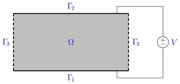
Figure 1: Model problem domain (two-dimensional depiction of actual three-dimensional, hexahedral domain). Boundary conditions: on $\Gamma_{1}$ (strong anchoring, Dirichlet boundary condition $\bm{n}=\bm{n}_{\text{b}}$ on $\bm{n}$, $\varphi=0$), on $\Gamma_{2}$ (weak anchoring, natural boundary condition $(\ref{eqn:strong})_{2}$ on $\bm{n}$, $\varphi=V$), on $\Gamma_{3}$ (periodic boundary conditions on both $\bm{n}$ and $\varphi$ on opposing sides of $\Gamma_{3}$).

with lower boundary $\Gamma_{1}$, upper boundary $\Gamma_{2}$, and lateral boundary $\Gamma_{3}$. A “strong anchoring condition” (Dirichlet boundary condition) is imposed on $\bm{n}$ on $\Gamma_{1}$, a “weak anchoring condition” (a natural boundary condition resulting from a surface anchoring energy) on $\Gamma_{2}$, and periodic boundary conditions on opposing sides of $\Gamma_{3}$. These cover the three types of boundary conditions typically encountered in modeling liquid crystal systems. The model domain may be viewed as a subdomain in a liquid crystal thin film regarded as having infinite extent in the lateral directions.

For a uniaxial nematic liquid crystal subject to a magnetic field (with boundary conditions as described above), the standard model free energy is an integral functional of the director field that can be taken in the form

(1) $$\mathcal{F}[\bm{n}]=\int_{\Omega}W(\bm{n},\nabla\bm{n})\,dV+\int_{\Gamma_{2}}W_{\text{s}}(\bm{n})\,dS,$$

where $W$ denotes the free-energy density (per unit volume) and $W_{\text{s}}$ the surface-anchoring energy (per unit area). The free-energy density consists of a part associated with distortional elasticity $W_{\text{e}}$ (for which we employ the classical Oseen-Frank formula) and a part associated with the magnetic induction, $W_{\text{H}}$:

$$W=W_{\text{e}}(\bm{n},\nabla\bm{n})+W_{\text{H}}(\bm{n}),$$

with

(2) $$2W_{\text{e}}=K_{1}(\operatorname{div}\bm{n})^{2}+K_{2}(\bm{n}\cdot\operatorname{curl}\bm{n})^{2}+K_{3}|\bm{n}\times\operatorname{curl}\bm{n}|^{2}+K_{24}\bigl{[}\operatorname{tr}(\nabla\bm{n})^{2}-(\operatorname{div}\bm{n})^{2}\bigr{]}.$$

Here $K_{1}$, $K_{2}$, $K_{3}$, and $K_{24}$ are material-dependent parameters (“elastic constants”), which under appropriate conditions ($0<K_{1},K_{2},K_{3}$ and $0<K_{24}<2\min\{K_{1},K_{2}\}$) guarantee that $W_{\text{e}}\geq 0$ and $W_{\text{e}}=0$ if and only if $\nabla\bm{n}=\mathbf{0}$. The constants $K_{1}$, $K_{2}$, and $K_{3}$ are referred to as the “splay,” “twist,” and “bend” constants, because of the simple types of distortions that they penalize (see [9, §3.1.1] or [38, §2.2] or [39, §3.3]); this terminology will come up in some of our examples. The $K_{24}$ term is a null Lagrangian and does not play a role in many simple systems. The precise form of $W_{\text{e}}$ does not matter to our development (though terms from it appear in examples that will follow). The simplest form for $W_{\text{e}}$ corresponds to $K_{1}=K_{2}=K_{3}=K_{24}=K$, which gives $W_{\text{e}}=\frac{1}{2}K|\nabla\bm{n}|^{2}$ (the “equal elastic constants model”).

The contribution to the free energy associated with the magnetic field (for materials of the type we study here) can be taken in the form

$$W_{\text{H}}=-\frac{1}{2}\chi_{\text{a}}(\bm{H}\cdot\bm{n})^{2},$$

with $\chi_{\text{a}}$ the diamagnetic anisotropy (a material-dependent parameter that can be positive or negative) and $\bm{H}$ the magnetic field (which can be assumed to be constant, as discussed in the Introduction). Globally stable configurations of the director field minimize $\mathcal{F}$ (subject to boundary conditions and the pointwise constraint $|\bm{n}|=1$); so $\chi_{\text{a}}>0$ encourages the director to be parallel to $\bm{H}$, while $\chi_{\text{a}}<0$ encourages it to be perpendicular to $\bm{H}$. The surface anchoring energy $W_{\text{s}}$ can take a variety of forms, a simple example being

$$W_{\text{s}}=-\frac{1}{2}W_{0}(\bm{n}\cdot\bm{n}_{\text{s}})^{2},$$

with $W_{0}$ the “anchoring strength.” With $W_{0}>0$, this encourages $\bm{n}$ to be parallel to the prescribed orientation $\bm{n}_{\text{s}}$ (the “easy axis”) on the boundary. See [17, §2.2, App. A.1] for more examples and references. The modeling aspects above are well documented in [9, §§3.1, 3.2], [38, §§2.2, 2.3, 2.6], and [39, §§3.2, 3.5, 4.1]. A summary of the relevant points is in [17, §2], from which we have adapted our model problems.

For a nematic liquid crystal subject to an electric field, the mutual influence of the electric field on the director field and of the director field on the electric field should be taken into account, as discussed in the Introduction. We do this by employing a free energy that is a functional of two state variables: the director field $\bm{n}$ and the electric potential field $\varphi$ (related to the electric field via $\bm{E}=-\nabla\varphi$). The free energy now takes the form

$$\mathcal{F}[\bm{n},\varphi]=\int_{\Omega}W(\bm{n},\nabla\bm{n},\nabla\varphi)\,dV+\int_{\Gamma_{2}}W_{\text{s}}(\bm{n})\,dS,$$

with

$$W=W_{\text{e}}(\bm{n},\nabla\bm{n})+W_{\text{E}}(\bm{n},\nabla\varphi).$$

Here $\Omega$, $\Gamma_{2}$, $W_{\text{e}}$, and $W_{\text{s}}$ are exactly as before, and the relevant relations from electrostatics are given by

(3) $$W_{\text{E}}=-\frac{1}{2}\bm{D}\cdot\bm{E},\quad\bm{D}={\bm{\epsilon}}(\bm{n})\bm{E},\quad{\bm{\epsilon}}=\epsilon_{0}(\epsilon_{\scriptscriptstyle\perp}\mathbf{I}+\epsilon_{\text{a}}\bm{n}\otimes\bm{n}),\quad\epsilon_{\text{a}}:=\epsilon_{\scriptscriptstyle\parallel}-\epsilon_{\scriptscriptstyle\perp}.$$

Here $\bm{D}$ is the electric displacement, ${{\bm{\epsilon}}}$ the dielectric tensor, $\epsilon_{0}$ the vacuum dielectric constant, and $\epsilon_{\scriptscriptstyle\parallel}$ and $\epsilon_{\scriptscriptstyle\perp}$ the material-dependent relative permittivities parallel to and perpendicular to the local director. The dielectric anisotropy $\epsilon_{\text{a}}$ can be positive or negative. The expression for $W_{\text{E}}$ is the correct electric contribution to the free energy associated with an electric field generated by electrodes held at constant potential in a transversely isotropic linear dielectric that contains no distribution of free charge. The electric potential $\varphi$ satisfies Dirichlet boundary conditions on $\Gamma_{1}$ and $\Gamma_{2}$ (of prescribed difference $V$) and periodic boundary conditions on opposing sides of $\Gamma_{3}$. For more discussion and additional references, see [9, §3.3], [38, §2.3.1], and [39, §4.1], or the synopsis in [17, §2.1].

To summarize, our two model free energies are

(4) $$\mathcal{F}_{\text{H}}[\bm{n}]=\int_{\Omega}\Bigl{[}W_{\text{e}}(\bm{n},\nabla\bm{n})-\frac{1}{2}\chi_{\text{a}}(\bm{H}\cdot\bm{n})^{2}\Bigr{]}dV+\int_{\Gamma_{2}}W_{\text{s}}(\bm{n})\,dS$$

(5) $$\mathcal{F}_{\text{E}}[\bm{n},\varphi]=\int_{\Omega}\Bigl{[}W_{\text{e}}(\bm{n},\nabla\bm{n})-\frac{1}{2}{\bm{\epsilon}}(\bm{n})\nabla\varphi\cdot\nabla\varphi\Bigr{]}dV+\int_{\Gamma_{2}}W_{\text{s}}(\bm{n})\,dS,$$

with $\Omega$ and $\Gamma_{2}$ as depicted in Fig. 1, $W_{\text{e}}$ as in Eq. 2, $W_{\text{s}}$ an appropriate surface anchoring energy, and ${{\bm{\epsilon}}}$ as in Eq. 3. Equilibrium fields are stationary points of these functionals (subject to the essential boundary conditions and the pointwise constraint $|\bm{n}|=1$), with globally stable phases corresponding to equilibrium fields of least free energy. The characterization of local stability of equilibria is the main topic that we take up in what follows. We note that since the dielectric tensor ${{\bm{\epsilon}}}$ is symmetric positive definite, the stationary points of $\mathcal{F}_{\text{E}}$ are maximizing with respect to $\varphi$, though they are locally minimizing with respect to $\bm{n}$.

In what follows, we assume that all admissible fields and admissible variations are regular enough to satisfy the various equilibrium characterizations in strong forms. We do this for simplicity and note that it precludes the presence of any singularities (“defects” or “disclinations”) in the systems we study. The models that we deal with are vectorial in nature with pointwise constraints and associated Lagrange multiplier fields of low regularity in the presence of defects. Weak variational formulations can require cumbersome technical assumptions—see, for example, [24, 25]. Let $C^{2}(\hskip 0.75pt\raisebox{7.58331pt}[0.0pt][0.0pt]{\makebox[0.0pt][l]{\rule{5.72223pt}{0.4pt}}}\Omega)$ denote real-valued scalar fields on $\Omega$ that are twice continuously differentiable with finite limits on $\partial\Omega$ (of the fields and their derivatives up to second order), and let $\bm{C}^{2}(\hskip 0.75pt\raisebox{7.58331pt}[0.0pt][0.0pt]{\makebox[0.0pt][l]{\rule{5.72223pt}{0.4pt}}}\Omega)$ denote the analogous space for vector fields on $\Omega$ (with values in real three-dimensional Euclidean space). Such fields are more than smooth enough for our purposes and are sufficient to ensure that the Lagrange multiplier fields we encounter will be bounded and continuous. We define our classes of admissible fields for $\bm{n}$ and $\varphi$ as follows:

$$\mathcal{N}=\bigl{\{}\bm{n}\in\bm{C}^{2}(\hskip 0.75pt\raisebox{7.58331pt}[0.0pt][0.0pt]{\makebox[0.0pt][l]{\rule{5.72223pt}{0.4pt}}}\Omega)\,\bigl{|}\,|\bm{n}|=1\text{ in }\Omega,\bm{n}=\bm{n}_{\text{b}}\text{ on }\Gamma_{1},\bm{n}\text{ periodic on }\Gamma_{3}\bigr{\}}$$

$${\Phi}=\bigl{\{}\varphi\in C^{2}(\hskip 0.75pt\raisebox{7.58331pt}[0.0pt][0.0pt]{\makebox[0.0pt][l]{\rule{5.72223pt}{0.4pt}}}\Omega)\,\bigl{|}\,\varphi=0\text{ on }\Gamma_{1},\varphi=V\text{ on }\Gamma_{2},\varphi\text{ periodic on }\Gamma_{3}\bigr{\}}.$$

Periodic here is taken to mean periodic on opposing sides of the lateral boundary of the hexahedral domain.

With our notation now defined, we can succinctly characterize globally stable solutions of our two models problems as follows:

$$\mathcal{F}_{\text{H}}[\bm{n}^{*}]=\min_{\bm{n}\in\mathcal{N}}\mathcal{F}_{\text{H}}[\bm{n}],\quad\mathcal{F}_{\text{E}}[\bm{n}^{*}\!\!,\varphi^{*}]=\min_{\bm{n}\in\mathcal{N}}\max_{\varphi\in\Phi}\mathcal{F}_{\text{H}}[\bm{n},\varphi].$$

Lacking convexity, these systems can have more than one globally stable solution. While the electric-field problems have an intrinsic minimax nature, their globally stable solutions still admit a characterization by a “least free energy principle”: a globally stable solution pair $\bm{n}^{*}$, $\varphi^{*}$ is an equilibrium pair of least free energy (among all equilibrium pairs). This point of view will be found to be useful in what follows.

3 Stability criteria for magnetic fields

If a liquid crystal system is sufficiently simple, then the local stability of an equilibrium director configuration of $\mathcal{F}_{\text{H}}$ can be analyzed by representing the director field in terms of one or two orientation angles (e.g., $\bm{n}=\cos\theta\,\bm{e}_{1}+\sin\theta\,\bm{e}_{2}$). Such representations free one from having to deal with the pointwise constraint $|\bm{n}|=1$ (which presents a complicating factor for numerical modeling, as well as for analysis). With the free energy expressed in terms of orientation angles, local stability is simply assessed in terms of the positive definiteness of the second variation of the free-energy functional. If, on the other hand, one chooses to (or needs to) model the director in terms of its components with respect some frame, then one must enforce $|\bm{n}|=1$ pointwise, and the Lagrange multiplier field associated with this enters both the equilibrium Euler-Lagrange equations as well as the criteria for local stability, as observed in [34] and as we shall see below.

Analyses using director components have been used in the past to study the stability of specific configurations, such as radial point defects (“hedgehogs”)—see, for example, [6, 7, 23, 27]. A stability criterion of a general nature is presented in [34], and it is closely related to our results for the case of a magnetic field (though here it is somewhat differently expressed and derived). A main contribution here is the extension of such ideas to systems involving coupled electric fields. Minimizing $\mathcal{F}_{\text{H}}$ subject to $|\bm{n}|=1$ can be viewed as the continuum analogue of a problem in equality-constrained optimization in $\mathbb{R}^{n}$, and we pursue this analogy, beginning with a recapitulation of the relevant formulas from that area.

3.1 Results from equality-constrained optimization theory

A discrete analogue of the constrained minimization problem for $\mathcal{F}_{\text{H}}$ is provided by the following:

$$\min_{\mathbf{x}\in\mathbb{R}^{n}}f(\mathbf{x}),\quad\text{subject to }g_{1}(\mathbf{x})=\cdots=g_{m}(\mathbf{x})=0.$$

Here the objective function $f$ and constraint functions $g_{1},\ldots,g_{m}$ are assumed to be real valued and smooth, and $\mathbb{R}^{n}$ denotes real $n$-dimensional Euclidean space with the standard inner product. The first-order and second-order necessary conditions associated with a local solution $\mathbf{x}_{0}$ are as follows. Under mild non-degeneracy conditions (such as linear independence of $\nabla g_{1}(\mathbf{x}_{0}),\ldots,\nabla g_{m}(\mathbf{x}_{0})$), there exist unique Lagrange multipliers $\lambda_{1}^{0},\ldots,\lambda_{m}^{0}\in\mathbb{R}$ such that

(6) $$\nabla f(\mathbf{x}_{0})=\lambda_{1}^{0}\nabla g_{1}(\mathbf{x}_{0})+\cdots+\lambda_{m}^{0}\nabla g_{m}(\mathbf{x}_{0})$$

and

(7a) $$\bigl{[}\nabla^{2}f(\mathbf{x}_{0})-\lambda_{1}^{0}\nabla^{2}g_{1}(\mathbf{x}_{0})-\cdots-\lambda_{m}^{0}\nabla^{2}g_{m}(\mathbf{x}_{0})\bigr{]}\mathbf{u}\cdot\mathbf{u}\geq 0,$$

for all $$\mathbf{u}\in\mathbb{R}^{n}$$ satisfying

(7b) $$\nabla g_{1}(\mathbf{x}_{0})\cdot\mathbf{u}=\cdots=\nabla g_{m}(\mathbf{x}_{0})\cdot\mathbf{u}=0.$$

That is to say, the constrained stationary point will be a local minimum only if the Hessian of the Lagrangian is positive semi definite on the tangent space to the constraint manifold at the point. Strict positivity in Eq. 7a for nontrivial $\mathbf{u}$ satisfying Eq. 7b is sufficient for local stability. We sketch below an approach to deriving these results that generalizes to our free-energy-minimization problems. The results can be found in standard references on optimization theory, such as [13, 19, 30, 31].

The conditions above can be deduced as follows. Give a trajectory $\mathbf{x}(t)$ on the constraint manifold through $\mathbf{x}_{0}$ smoothly parametrized by $t$:

$$g_{1}(\mathbf{x}(t))=\cdots=g_{m}(\mathbf{x}(t))=0,\quad-c<t<c,\text{ some }c>0,\quad\mathbf{x}(0)=\mathbf{x}_{0}.$$

With the definition $F(t):=f(\mathbf{x}(t))$, the point $\mathbf{x}_{0}$ being a local minimum implies $F^{\prime}(0)=0$ and $F^{\prime\prime}(0)\geq 0$. Now

$$F^{\prime}(0)=\nabla f(\mathbf{x}_{0})\cdot\dot{\mathbf{x}}_{0}~{}~{}\text{and}~{}~{}F^{\prime\prime}(0)=\nabla f(\mathbf{x}_{0})\cdot\ddot{\mathbf{x}}_{0}+\nabla^{2}f(\mathbf{x}_{0})\dot{\mathbf{x}}_{0}\cdot\dot{\mathbf{x}}_{0},$$

where

$$\dot{\mathbf{x}}_{0}:=\frac{d}{dt}\mathbf{x}(t)\bigr{|}_{t=0}~{}~{}\text{and}~{}~{}\ddot{\mathbf{x}}_{0}:=\frac{d^{2}}{dt^{2}}\mathbf{x}(t)\bigr{|}_{t=0}.$$

For each of the constraints, we have

$$g_{i}(\mathbf{x}(t))=0~{}\Rightarrow~{}\frac{d}{dt}g_{i}(\mathbf{x}(t))=\frac{d^{2}}{dt^{2}}g_{i}(\mathbf{x}(t))=\cdots=0,~{}-c<t<c,$$

from which we obtain,

$$\nabla g_{i}(\mathbf{x}_{0})\cdot\dot{\mathbf{x}}_{0}=0,~{}~{}\nabla g_{i}(\mathbf{x}_{0})\cdot\ddot{\mathbf{x}}_{0}+\nabla^{2}g_{i}(\mathbf{x}_{0})\dot{\mathbf{x}}_{0}\cdot\dot{\mathbf{x}}_{0}=0,~{}~{}\text{for }i=1,\ldots,m.$$

Thus $\dot{\mathbf{x}}_{0}$ is in the tangent space to the constraint manifold at $\mathbf{x}_{0}$, and stationarity implies $F^{\prime}(0)=\nabla f(\mathbf{x}_{0})\cdot\dot{\mathbf{x}}_{0}=0$, for all such $\dot{\mathbf{x}}_{0}$ as well. Assuming the constraint normals $\nabla g_{1}(\mathbf{x}_{0}),\ldots,\nabla g_{m}(\mathbf{x}_{0})$ to be linearly independent, for example, this guarantees that $\nabla f(\mathbf{x}_{0})$ has a unique representation as a linear combination of $\nabla g_{1}(\mathbf{x}_{0}),\ldots,\nabla g_{m}(\mathbf{x}_{0})$, i.e., Eq. 6 holds with unique $\lambda_{1}^{0},\ldots,\lambda_{m}^{0}$. This relation and the second part of the relations above can be used to simplify the requirement

$$0\leq F^{\prime\prime}(0)=\nabla f(\mathbf{x}_{0})\cdot\ddot{\mathbf{x}}_{0}+\nabla^{2}f(\mathbf{x}_{0})\dot{\mathbf{x}}_{0}\cdot\dot{\mathbf{x}}_{0}$$

via

$$\nabla f(\mathbf{x}_{0})\cdot\ddot{\mathbf{x}}_{0} =\lambda_{1}^{0}\nabla g_{1}(\mathbf{x}_{0})\cdot\ddot{\mathbf{x}}_{0}+\cdots+\lambda_{m}^{0}\nabla g_{m}(\mathbf{x}_{0})\cdot\ddot{\mathbf{x}}_{0}$$

$$=-\lambda_{1}^{0}\nabla^{2}g_{1}(\mathbf{x}_{0})\dot{\mathbf{x}}_{0}\cdot\dot{\mathbf{x}}_{0}-\cdots-\lambda_{m}^{0}\nabla^{2}g_{m}(\mathbf{x}_{0})\dot{\mathbf{x}}_{0}\cdot\dot{\mathbf{x}}_{0}.$$

Substituting this into the inequality on $F^{\prime\prime}(0)$ above leads to the second-order necessary condition Eq. 7. One anticipates that it should be possible to frame the statements and analysis of our continuum liquid crystal models in a similar way, and we endeavor to do so below.

3.2 Stability criteria

We seek to establish similar conditions for a local minimum $\bm{n}_{0}$ of a functional of the form Eq. 1,

$$\mathcal{F}[\bm{n}]=\int_{\Omega}W(\bm{n},\nabla\bm{n})\,dV+\int_{\Gamma_{2}}W_{\text{s}}(\bm{n})\,dS,$$

with $\Omega$ and $\Gamma_{2}$ as in Fig. 1, $W$ an appropriate free-energy density, and $W_{\text{s}}$ an appropriate anchoring energy, subject to the essential boundary conditions of our model problems (Dirichlet on $\Gamma_{1}$, periodic on $\Gamma_{3}$), and subject to the pointwise constraint $|\bm{n}|=1$. This includes the model free energy $\mathcal{F}_{\text{H}}$ in Eq. 4. Let $\bm{n}_{\varepsilon}$ be a family of unit-length vector fields on $\Omega$ smoothly parametrized by $\varepsilon$ such that

$$|\bm{n}_{\varepsilon}|=1,~{}~{}-c<\varepsilon<c,\text{ some }c>0,~{}~{}\bm{n}_{\varepsilon}|_{\varepsilon=0}=\bm{n}_{0}.$$

The most commonly used realization of such a field is

(8) $$\bm{n}_{\varepsilon}=\frac{\bm{n}_{0}+\varepsilon\bm{v}}{|\bm{n}_{0}+\varepsilon\bm{v}|},$$

where $\bm{v}$ is such that the combination $\bm{n}_{0}+\varepsilon\bm{v}$ satisfies the same essential boundary conditions and regularity assumptions that $\bm{n}_{0}$ must satisfy but is otherwise arbitrary. With the definition $F(\varepsilon):=\mathcal{F}[\bm{n}_{\varepsilon}]$, the point $\bm{n}_{0}$ being a local minimum point implies $F^{\prime}(0)=0$ and $F^{\prime\prime}(0)\geq 0$. Here

$$F^{\prime}(0)=\delta\mathcal{F}[\bm{n}_{0}](\dot{\bm{n}}_{0})~{}~{}\text{and}~{}~{}F^{\prime\prime}(0)=\delta\mathcal{F}[\bm{n}_{0}](\ddot{\bm{n}}_{0})+\delta^{2}\!\mathcal{F}[\bm{n}_{0}](\dot{\bm{n}}_{0}),$$

with $\delta\mathcal{F}$ and $\delta^{2}\!\mathcal{F}$ the first and second variations,

$$\delta\mathcal{F}[\bm{n}](\bm{v})=\frac{d}{d\varepsilon}\mathcal{F}[\bm{n}+\varepsilon\bm{v}]\bigr{|}_{\varepsilon=0}~{}~{}\text{and}~{}~{}\delta^{2}\!\mathcal{F}[\bm{n}](\bm{v})=\frac{d^{2}}{d\varepsilon^{2}}\mathcal{F}[\bm{n}+\varepsilon\bm{v}]\bigr{|}_{\varepsilon=0},$$

giving

$$\delta\mathcal{F}[\bm{n}](\bm{v}) =\int_{\Omega}\Bigl{(}\frac{\partial W}{\partial\bm{n}}\cdot\bm{v}+\frac{\partial W}{\partial\nabla\bm{n}}\cdot\nabla\bm{v}\Bigr{)}\,dV+\int_{\Gamma_{2}}\Bigl{(}\frac{\partial W_{\text{s}}}{\partial\bm{n}}\cdot\bm{v}\Bigr{)}\,dS$$

$$=\int_{\Omega}\Bigl{(}\frac{\partial W}{\partial n_{i}}v_{i}+\frac{\partial W}{\,\partial n_{i,j}}v_{i,j}\Bigr{)}\,dV+\int_{\Gamma_{2}}\Bigl{(}\frac{\partial W_{\text{s}}}{\partial n_{i}}v_{i}\Bigr{)}\,dS$$

and

$$\delta^{2}\!\mathcal{F}[\bm{n}](\bm{v})=\int_{\Omega}\Bigl{(}\frac{\partial^{2}W}{\partial n_{i}\partial n_{k}}v_{i}v_{k}+2\frac{\partial^{2}W}{\partial n_{i}\partial n_{k,l}}v_{i}v_{k,l}+\frac{\partial^{2}W}{\partial n_{i,j}\partial n_{k,l}}v_{i,j}v_{k,l}\Bigr{)}\,dV\\ {}+\int_{\Gamma_{2}}\Bigl{(}\frac{\partial^{2}W}{\partial n_{i}\partial n_{k}}v_{i}v_{k}\Bigr{)}\,dS,$$

where

$$\dot{\bm{n}}_{0}:=\frac{d}{d\varepsilon}\bm{n}_{\varepsilon}\bigr{|}_{\varepsilon=0}~{}~{}\text{and}~{}~{}\ddot{\bm{n}}_{0}:=\frac{d^{2}}{d\varepsilon^{2}}\bm{n}_{\varepsilon}\bigr{|}_{\varepsilon=0}.$$

Here $n_{i}$ and $v_{i}$ are the components of $\bm{n}$ and $\bm{v}$ with respect to a fixed Cartesian frame, $n_{i,j}=\partial n_{i}/\partial x_{j}$, etc., and summation over repeated indices is implied. We note that with $\bm{n}_{\varepsilon}$ defined as in Eq. 8, we would have

$$\dot{\bm{n}}_{0}=\mathbf{P}(\bm{n}_{0})\bm{v},\quad\mathbf{P}(\bm{n}):=\mathbf{I}-\bm{n}\otimes\bm{n}.$$

Given a unit-length vector field $\bm{n}$, the tensor field $\mathbf{P}(\bm{n})$ defined above projects transverse to $\bm{n}$ at each point [39, §2.5] and is a convenient operator in the analysis of director models.

Differentiations with respect to $\varepsilon$ of $|\bm{n}_{\varepsilon}|^{2}=\bm{n}_{\varepsilon}\cdot\bm{n}_{\varepsilon}=1$ give rise to the pointwise relations

$$\bm{n}_{0}\cdot\dot{\bm{n}}_{0}=0,\quad\bm{n}_{0}\cdot\ddot{\bm{n}}_{0}+|\dot{\bm{n}}_{0}|^{2}=0.$$

Any such $\dot{\bm{n}}_{0}$ necessarily vanishes on $\Gamma_{1}$, is periodic on opposing sides of $\Gamma_{3}$, and is transverse to $\bm{n}_{0}$ (in the sense that $\bm{n}_{0}\cdot\dot{\bm{n}}_{0}=0$ on $\Omega$). We denote the collection of all such vector fields

$$\mathcal{U}_{0}=\bigl{\{}\bm{u}\in\bm{C}^{2}(\hskip 0.75pt\raisebox{7.58331pt}[0.0pt][0.0pt]{\makebox[0.0pt][l]{\rule{5.72223pt}{0.4pt}}}\Omega)\,\bigl{|}\,\bm{u}=\mathbf{0}\text{ on }\Gamma_{1},\bm{u}\text{ periodic on }\Gamma_{3},\bm{n}_{0}\cdot\bm{u}=0\text{ on }\Omega\bigr{\}}.$$

Such vector fields can be generated from the larger class

$$\mathcal{V}_{0}=\bigl{\{}\bm{v}\in\bm{C}^{2}(\hskip 0.75pt\raisebox{7.58331pt}[0.0pt][0.0pt]{\makebox[0.0pt][l]{\rule{5.72223pt}{0.4pt}}}\Omega)\,\bigl{|}\,\bm{v}=\mathbf{0}\text{ on }\Gamma_{1},\bm{v}\text{ periodic on }\Gamma_{3}\bigr{\}}$$

by using the transverse projector $\mathbf{P}(\bm{n}_{0})$ above:

$$\bm{u}\in\mathcal{U}_{0}~{}\Leftrightarrow~{}\bm{u}=\mathbf{P}(\bm{n}_{0})\bm{v},\text{ some }\bm{v}\in\mathcal{V}_{0}.$$

The first-order necessary conditions follow from

$$F^{\prime}(0)=0~{}\Rightarrow~{}\delta\mathcal{F}[\bm{n}_{0}](\bm{u})=0,~{}\forall\bm{u}\in\mathcal{U}_{0},$$

which (using $\bm{u}=\mathbf{P}(\bm{n}_{0})\bm{v}$ and integration by parts) can be written in the following equivalent forms:

(9) $$\delta\mathcal{F}[\bm{n}_{0}](\bm{v})=\int_{\Omega}\lambda_{0}\bm{n}_{0}\cdot\bm{v}\,dV+\int_{\Gamma_{2}}\mu_{0}\bm{n}_{0}\cdot\bm{v}\,dS,~{}~{}\forall\bm{v}\in\mathcal{V}_{0}$$

or

(10) $$-\operatorname{div}\Bigl{(}\frac{\partial W}{\partial\nabla\bm{n}}\Bigr{)}+\frac{\partial W}{\partial\bm{n}}=\lambda_{0}\bm{n}_{0}\text{ in }\Omega,\quad\Bigl{(}\frac{\partial W}{\partial\nabla\bm{n}}\Bigr{)}\bm{\nu}+\frac{\partial W_{\text{s}}}{\partial\bm{n}}=\mu_{0}\bm{n}_{0}\text{ on }\Gamma_{2}.$$

Equation 9 is the analogue of Eq. 6. The role of the constraint functions $g_{i}$ and their gradients is here played by

$$g(\bm{n})=\frac{1}{2}\bigl{(}|\bm{n}|^{2}-1\bigr{)},\text{ for which }\frac{\partial g}{\partial\bm{n}}=\bm{n},~{}\frac{\partial^{2}g}{\,\partial\bm{n}^{2}}=\mathbf{I}.$$

The Lagrange multiplier fields $\lambda_{0}$ and $\mu_{0}$ are given by

$$\lambda_{0}=\Bigl{[}-\operatorname{div}\Bigl{(}\frac{\partial W}{\partial\nabla\bm{n}}\Bigr{)}+\frac{\partial W}{\partial\bm{n}}\Bigr{]}\cdot\bm{n}_{0},\quad\mu_{0}=\Bigl{[}\Bigl{(}\frac{\partial W}{\partial\nabla\bm{n}}\Bigr{)}\bm{\nu}+\frac{\partial W_{\text{s}}}{\partial\bm{n}}\Bigr{]}\cdot\bm{n}_{0},$$

with the bracketed expressions evaluated on the equilibrium field $\bm{n}_{0}$. The results above are well known; the only point here is to highlight the analogy to the discrete setting and to anticipate the next steps.

The second-order necessary conditions follow from

$$F^{\prime\prime}(0)\geq 0~{}~{}\Rightarrow~{}~{}\delta\mathcal{F}[\bm{n}_{0}](\ddot{\bm{n}}_{0})+\delta^{2}\mathcal{F}[\bm{n}_{0}](\dot{\bm{n}}_{0})\geq 0.$$

The weak-form Euler-Lagrange equation Eq. 9 and the pointwise relation $\bm{n}_{0}\cdot\ddot{\bm{n}}_{0}+|\dot{\bm{n}}_{0}|^{2}=0$ can be used to simplify this as follows,

$$\delta\mathcal{F}[\bm{n}_{0}](\ddot{\bm{n}}_{0}) =\int_{\Omega}\lambda_{0}\bm{n}_{0}\cdot\ddot{\bm{n}}_{0}\,dV+\int_{\Gamma_{2}}\mu_{0}\bm{n}_{0}\cdot\ddot{\bm{n}}_{0}\,dS$$

$$=-\int_{\Omega}\lambda_{0}|\dot{\bm{n}}_{0}|^{2}\,dV-\int_{\Gamma_{2}}\mu_{0}|\dot{\bm{n}}_{0}|^{2}\,dS,$$

which leads to

(11) $$\delta^{2}\!\mathcal{F}[\bm{n}_{0}](\bm{u})-\int_{\Omega}\lambda_{0}|\bm{u}|^{2}\,dV-\int_{\Gamma_{2}}\mu_{0}|\bm{u}|^{2}\,dS\geq 0,~{}~{}\forall\bm{u}\in\mathcal{U}_{0}.$$

The above, then, is our necessary condition for local stability of $\bm{n}_{0}$, the analogue of Eq. 7. Positive definiteness of the quadratic form in Eq. 11, in the sense

$$\delta^{2}\!\mathcal{F}[\bm{n}_{0}](\bm{u})-\int_{\Omega}\lambda_{0}|\bm{u}|^{2}\,dV-\int_{\Gamma_{2}}\mu_{0}|\bm{u}|^{2}\,dS\geq c\int_{\Omega}|\bm{u}|^{2}\,dV,~{}~{}\forall\bm{u}\in\mathcal{U}_{0},\text{ some }c>0,$$

would be sufficient for local stability. Viewed in terms of expansions, we have

$$\mathcal{F}[\bm{n}_{\varepsilon}]=\mathcal{F}[\bm{n}_{0}]+\frac{1}{2}\varepsilon^{2}\biggl{[}\delta^{2}\!\mathcal{F}[\bm{n}_{0}](\dot{\bm{n}}_{0})-\int_{\Omega}\lambda_{0}|\dot{\bm{n}}_{0}|^{2}\,dV-\int_{\Gamma_{2}}\mu_{0}|\dot{\bm{n}}_{0}|^{2}\,dS\biggr{]}+o(\varepsilon^{2}),$$

for $\bm{n}_{0}\in\mathcal{N}_{0}$ satisfying Eq. 9. The approach taken here is classical. It is, in essence, that of [8, §§IV.7.2, IV.8.1], used in the setting of liquid crystals in [39, §3.5]. Similar results, derived instead in terms of expansions, are found in [34].

3.3 Examples

We illustrate the application of the stability criterion above to some examples, some of which will be considered again later in the context of electric fields. We first observe that when the ground state $\bm{n}_{0}$ is uniform (which is the case in all the classical Fréedericksz transitions), then the second variation of the magnetic-field model free energy Eq. 4 takes the simple form

$$\delta^{2}\!\mathcal{F}_{\text{H}}[\bm{n}_{0}](\bm{u})=\int_{\Omega}\bigl{[}K_{1}(\operatorname{div}\bm{u})^{2}+K_{2}(\bm{n}_{0}\cdot\operatorname{curl}\bm{u})^{2}+K_{3}|\bm{n}_{0}\times\operatorname{curl}\bm{u}|^{2}-\chi_{\text{a}}(\bm{H}\cdot\bm{u})^{2}\bigr{]}\,dV.$$

Here we have dropped the $K_{24}$ term and the term associated with the anchoring energy on $\Gamma_{2}$, since neither will appear in our examples below. It is also the case that if $\bm{n}_{0}$ is uniform and in addition $\bm{n}_{0}\perp\bm{H}$ (which is the case in all the classical Fréedericksz transitions with $\chi_{\text{a}}>0$), then it necessarily follows that the associated equilibrium Lagrange multiplier field $\lambda_{0}$ will be zero.

3.3.1 Classical Fréedericksz transitions

We consider three of the classical Fréedericksz geometries, as shown in Fig. 2.

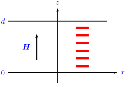
(a) splay geometry ($\chi_{\text{a}}>0$)

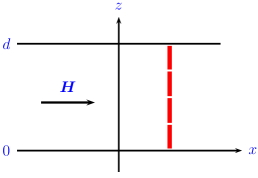
(b) bend geometry ($\chi_{\text{a}}>0$)

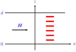
(c) in-plane geometry ($\chi_{\text{a}}<0$)

Figure 2: Three geometries of example magnetic-field Fréedericksz transitions. The liquid crystal film is confined to $0<z<d$. The ground state equilibrium solutions $\bm{n}_{0}$ are indicated, as are the orientations of the magnetic fields and the signs of the diamagnetic anisotropy $\chi_{\text{a}}$. Strong anchoring (Dirichlet boundary conditions) on the director field $\bm{n}$ is assumed on $z=0$ and $z=d$.

Figure 2a depicts the “splay Fréedericksz geometry.” With the director field $\bm{n}$ assumed to be uniform in the lateral directions and confined to the tilt plane spanned by $\bm{e}_{x}$ and $\bm{e}_{z}$,

$$\bm{n}=n_{x}(z)\bm{e}_{x}+n_{z}(z)\bm{e}_{z},$$

the free energy (per unit cross-sectional area) is given by

$$\mathcal{F}[\bm{n}]=\frac{1}{2}\int_{0}^{d}\bigl{(}K_{1}n_{z,z}^{2}+K_{3}n_{x,z}^{2}-\chi_{\text{a}}H^{2}n_{z}^{2}\bigr{)}\,dz.$$

Here $n_{z,z}$ denotes $\frac{d}{dz}n_{z}$, etc. The Euler-Lagrange equations are

$$K_{3}n_{x,zz}+\lambda n_{x}=0,~{}~{}K_{1}n_{z,zz}+\bigl{(}\chi_{\text{a}}H^{2}+\lambda\bigr{)}n_{z}=0,~{}~{}n_{x}^{2}+n_{z}^{2}=1,$$

and the ground state solution is

$$\bm{n}_{0}=\bm{e}_{x},~{}~{}\lambda_{0}=0.$$

Thus, in terms of components, the ground state is $n_{x}=1$, $n_{z}=0$ (which satisfy the Euler-Lagrange equations in a trivial way), and we note that $\bm{n}_{0}=-\bm{e}_{x}$ would work equally well. The second variation (with $\bm{u}=u(z)\bm{e}_{x}+w(z)\bm{e}_{z}$ restricted to the same tilt plane as $\bm{n}$) is given by

$$\delta^{2}\!\mathcal{F}[\bm{n}_{0}](\bm{u})=\int_{0}^{d}\bigl{(}K_{1}w_{z}^{2}+K_{3}u_{z}^{2}-\chi_{\text{a}}H^{2}w^{2}\bigr{)}\,dz.$$

For unsubscripted scalar fields, we denote $w_{z}=dw/dz$ (or $w_{z}=\partial w/\partial z$, as the situation may require), etc. Admissible variations ($\bm{u}\in\mathcal{U}_{0}$) must satisfy $\bm{n}_{0}\cdot\bm{u}=0$, which implies that $u=0$ and $\bm{u}=w(z)\bm{e}_{z}$. The stability condition Eq. 11 thus becomes

$$\int_{0}^{d}\bigl{(}K_{1}w_{z}^{2}-\chi_{\text{a}}H^{2}w^{2}\bigr{)}\,dz\geq 0~{}\Leftrightarrow~{}\frac{\chi_{\text{a}}H^{2}}{K_{1}}\leq\frac{\int_{0}^{d}w_{z}^{2}\,dz}{\int_{0}^{d}w^{2}\,dz},$$

for all smooth $w$ such that $w(0)=w(d)=0$. The minimum of the Rayleigh quotient on the right-hand side above (over smooth $w$ satisfying $w(0)=w(d)=0$) is $\pi^{2}/d^{2}$, which finally leads to

$$H\leq\frac{\pi}{d}\sqrt{\frac{K_{1}}{\chi_{\text{a}}}}=:H_{\text{c}},$$

the correct instability threshold for this problem [9, (3.64)], [38, (3.126)], [39, (4.43)].

In a very similar way, the magnetic-field bend-Fréedericksz transition (depicted in Fig. 2b) has a ground state

$$\bm{n}_{0}=\bm{e}_{z},~{}~{}\lambda_{0}=0$$

and a second variation given by

$$\delta^{2}\!\mathcal{F}[\bm{n}_{0}](\bm{u})=\int_{0}^{d}\bigl{(}K_{1}w_{z}^{2}+K_{3}u_{z}^{2}-\chi_{\text{a}}H^{2}u^{2}\bigr{)}\,dz.$$

With $\bm{n}_{0}\cdot\bm{u}=0$ implying $w=0$, Eq. 11 leads to

$$\int_{0}^{d}\bigl{(}K_{3}u_{z}^{2}-\chi_{\text{a}}H^{2}u^{2}\bigr{)}\,dz\geq 0,$$

for all smooth $u$ such that $u(0)=u(d)=0$, giving

$$H\leq\frac{\pi}{d}\sqrt{\frac{K_{3}}{\chi_{\text{a}}}}=:H_{\text{c}}.$$

This again is the correct instability threshold [9, (3.64)], [38, (3.143)], [39, §4.2.4]. Here we have again assumed that $\bm{n}$ is restricted to $\operatorname{span}\{\bm{e}_{x},\bm{e}_{z}\}$ and is uniform in the lateral directions. These two examples will be expanded upon below, where we relax some assumptions; they also will be revisited later with the systems subjected to electric fields (instead of magnetic fields), in which case the splay transition will behave as one would naively expect, but the bend transition will not.

A final classical Fréedericksz transition, depicted in Fig. 2c, illustrates the role of a non-vanishing Lagrange multiplier field $\lambda_{0}$. We again assume that $\bm{n}$ is restricted to $\operatorname{span}\{\bm{e}_{x},\bm{e}_{z}\}$ and is uniform in lateral directions, but here we now assume that $\chi_{\text{a}}<0$ (which encourages $\bm{n}$ to orient perpendicular to $\bm{H}$). We note that another simple distortion is possible here involving a twisting of the director parallel to the $x$-$y$ plane, but we do not consider this at the present time. With our assumptions, the free energy and Euler-Lagrange equations are given by

$$\mathcal{F}[\bm{n}]=\frac{1}{2}\int_{0}^{d}\bigl{(}K_{1}n_{z,z}^{2}+K_{3}n_{x,z}^{2}-\chi_{\text{a}}H^{2}n_{x}^{2}\bigr{)}\,dz$$

$$K_{3}n_{x,zz}+(\chi_{\text{a}}H^{2}+\lambda)n_{x}=0,~{}~{}K_{1}n_{z,zz}+\lambda n_{z}=0,~{}~{}n_{x}^{2}+n_{z}^{2}=1,$$

with ground state

$$\bm{n}_{0}=\bm{e}_{x},~{}~{}\lambda_{0}=-\chi_{\text{a}}H^{2}.$$

The Lagrange multiplier field $\lambda_{0}$ is constant here, due to the simplicity of the configuration; it need not be so in general. The constraint $\bm{n}_{0}\cdot\bm{u}=0$ gives

$$\bm{u}=w(z)\bm{e}_{z}~{}\Rightarrow~{}\operatorname{div}\bm{u}=w_{z},~{}\operatorname{curl}\bm{u}=\mathbf{0},~{}\bm{H}\cdot\bm{u}=0,$$

so that the stability condition Eq. 11 becomes

$$\delta^{2}\!\mathcal{F}[\bm{n}_{0}](\bm{u})-\int_{0}^{d}\lambda_{0}|\bm{u}|^{2}\,dz=K_{1}\!\int_{0}^{d}\!w_{z}^{2}\,\,dz+\chi_{\text{a}}H^{2}\!\int_{0}^{d}\!w^{2}\,dz\geq 0,$$

giving

$$-\frac{\chi_{\text{a}}H^{2}}{K_{1}}\leq\frac{\int_{0}^{d}w_{z}^{2}\,dz}{\int_{0}^{d}w^{2}\,dz}~{}\Rightarrow~{}H\leq\frac{\pi}{d}\sqrt{\frac{K_{1}}{-\chi_{\text{a}}\,}}=:H_{\text{c}}.$$

3.3.2 Periodic instabilities

It is possible for simple systems, such as those depicted in Fig. 2, to exhibit instabilities with more structure, such as periodic modulations in the plane of the liquid crystal film. We consider two such examples: the “stripe phase” of Allender, Hornreich, and Johnson [1] and the periodic instability of Lonberg and Meyer [29]. In both cases, we must relax the constraints we imposed in the examples above (i.e., uniformity of the director in lateral directions and confinement of it to a fixed tilt plane).

The stripe phase occurs in the bend-Fréedericksz geometry (Fig. 2b). The ground state is as before:

$$\bm{n}_{0}=\bm{e}_{z},~{}~{}\lambda_{0}=0.$$

The admissible variations ($\bm{n}_{0}\cdot\bm{u}=0$), however, are now taken in the form

$$\bm{u}=u(y,z)\bm{e}_{x}+v(y,z)\bm{e}_{y}.$$

The domain $\Omega$ is taken as one periodic cell

$$\Omega=\{(y,z)|-L<y<L,~{}0<z<d\},$$

with $u$ and $v$ periodic in $y$ (of period $2L$), vanishing on $z=0$ and $z=d$. The actual periodicity of a periodic equilibrium solution is chosen spontaneously by the system; thus $L$ would not be known a-priori—see Appendix A for how this issue can be addressed in the context of the next example.

Using the assumptions above, we obtain

$$\delta^{2}\!\mathcal{F}[\bm{n}_{0}](\bm{u})=\int_{\Omega}\bigl{[}K_{1}v_{y}^{2}+K_{2}u_{y}^{2}+K_{3}\bigl{(}u_{z}^{2}+v_{z}^{2}\bigr{)}-\chi_{\text{a}}H^{2}u^{2}\bigr{]}\,dA,$$

leading to the stability condition

(12) $$\int_{0}^{d}\int_{-L}^{L}\bigl{(}K_{2}u_{y}^{2}+K_{3}u_{z}^{2}-\chi_{\text{a}}H^{2}u^{2}\bigr{)}\,dy\,dz+\int_{0}^{d}\int_{-L}^{L}\bigl{(}K_{1}v_{y}^{2}+K_{3}v_{z}^{2}\bigr{)}\,dy\,dz\geq 0,$$

for all $u,v\in C^{2}(\hskip 0.75pt\raisebox{7.58331pt}[0.0pt][0.0pt]{\makebox[0.0pt][l]{\rule{5.72223pt}{0.4pt}}}\Omega)$, periodic in $y$ (of period $2L$), vanishing on $z=0$ and $z=d$. It is clear by inspection that the derivatives in $y$ and the $v$ component in general can only elevate the value of the quadratic form, leading to the conclusion that there can be no instability of $\bm{n}_{0}$ to a periodic-in-$y$ mode and that the first instability encountered is the classical Fréedericksz transition

$$u=\sin\frac{\pi z}{d},~{}~{}v=0,~{}~{}H_{\text{c}}=\frac{\pi}{d}\sqrt{\frac{K_{3}}{\chi_{\text{a}}}}.$$

In fact, the stripe phase enters as a secondary bifurcation off the branch of these classical solutions [1] (further explored in [20, 35, 36]). In more quantitative terms, the quadratic form Eq. 12 is diagonalized by the modes

$$f_{mn}=\exp\Bigl{(}i\frac{m\pi y}{L}\Bigr{)}\sin\frac{n\pi z}{d},~{}~{}m=0,\pm 1,\pm 2,\ldots,~{}n=1,2,\ldots,$$

with

$$u=f_{mn},~{}~{}v=0,~{}~{}\lambda_{mn}=K_{2}\frac{m^{2}\pi^{2}}{L^{2}}+K_{3}\frac{n^{2}\pi^{2}}{d^{2}}-\chi_{\text{a}}H^{2}$$

and

$$u=0,~{}~{}v=f_{mn},~{}~{}\lambda_{mn}=K_{1}\frac{m^{2}\pi^{2}}{L^{2}}+K_{3}\frac{n^{2}\pi^{2}}{d^{2}},$$

with the leading instability mode corresponding to $u=f_{01}$, $v=0$. The reason things are so simple here is that $u$ and $v$ are uncoupled.

The periodic instability of Lonberg and Meyer [29] is more complicated and exhibits different behavior. The geometry is the splay-Fréedericksz geometry (Fig. 2a). With ground state

$$\bm{n}_{0}=\bm{e}_{x},~{}~{}\lambda_{0}=0,$$

admissible variations now taken in the form

$$\bm{u}=v(y,z)\bm{e}_{y}+w(y,z)\bm{e}_{z},$$

and domain $\Omega$ taken to be one periodic cell (as in the previous example), the stability condition Eq. 11 becomes

(13) $$\int_{0}^{d}\int_{-L}^{L}\bigl{[}K_{1}(v_{y}+w_{z})^{2}+K_{2}(v_{z}-w_{y})^{2}-\chi_{\text{a}}H^{2}w^{2}\bigr{]}\,dy\,dz\geq 0,$$

for all $v,w\in C^{2}(\hskip 0.75pt\raisebox{7.58331pt}[0.0pt][0.0pt]{\makebox[0.0pt][l]{\rule{5.72223pt}{0.4pt}}}\Omega)$, periodic in $y$ (with period $2L$), vanishing on $z=0$ and $z=d$. The fields $v$ and $w$ are coupled now, and so the quadratic form is not diagonalized by simple Fourier expansions. In addition to experiments and theory presented in [29], one finds results in the brief note [32]; while in [39, §4.3], the system is studied as an example of a “periodic Freedericks transition.” We present a somewhat different analysis in Appendix A and summarize the main results now.

The experiments reported in [29] used polymer liquid crystal materials, which are characterized by very elongated “rod like” molecular architecture and by having “twist” elastic constants, $K_{2}$ in Eq. 2, that are small compared to their “splay” elastic constants, $K_{1}$. For such materials, the authors reported that the classical Fréedericksz transition was preceded (at a lower magnetic-field strength) by an instability to a solution that was periodic in $y$, with a period chosen by the system. Analysis of the model formulated above confirms this. There is a value $\hskip 1.75pt\raisebox{7.83331pt}[0.0pt][0.0pt]{\makebox[0.0pt][l]{\rule{7.45833pt}{0.4pt}}}K_{2}^{*}\doteq 0.303$ (which can be determined analytically) such that for $K_{2}/K_{1}<\hskip 1.75pt\raisebox{7.83331pt}[0.0pt][0.0pt]{\makebox[0.0pt][l]{\rule{7.45833pt}{0.4pt}}}K_{2}^{*}$, the uniform ground state $\bm{n}_{0}$ will become unstable to a periodic-in-$y$ solution of some period for some $H_{\text{p}}<H_{\text{c}}$. As $K_{2}/K_{1}\rightarrow\hskip 1.75pt\raisebox{7.83331pt}[0.0pt][0.0pt]{\makebox[0.0pt][l]{\rule{7.45833pt}{0.4pt}}}K_{2}^{*}$, $H_{\text{p}}\rightarrow H_{\text{c}}$, and the period of the instability mode becomes infinite. See Appendix A for details.

The examples in this section do not provide new information about these systems. They merely demonstrate consistency with known results, using the framework that has been developed here. Also, the essential role in our framework of the Lagrange multiplier field, when it is nonzero, has been made clear. The extension of these ideas to systems involving electric fields is taken up next.

4 Stability criteria for electric fields

In extending the results of the previous section to the case of a liquid-crystal system subjected to an electric field, we take into account the inhomogeneous nature of the electric field (in general) and its coupling to the director field, and we work with a model free energy of the form Eq. 5:

$$\mathcal{F}[\bm{n},\varphi]=\int_{\Omega}\Bigl{[}W_{\text{e}}(\bm{n},\nabla\bm{n})-\frac{1}{2}{\bm{\epsilon}}(\bm{n})\nabla\varphi\cdot\nabla\varphi\Bigr{]}dV+\int_{\Gamma_{2}}W_{\text{s}}(\bm{n})\,dS.$$

This now is a function of two state variables: $\bm{n}$ (the director field) and $\varphi$ (the electric potential). The dielectric tensor ${{\bm{\epsilon}}}$ is as given in Eq. 3, with $\epsilon_{\scriptscriptstyle\perp},\epsilon_{\scriptscriptstyle\parallel}>0$. It follows that for any unit-length vector field $\bm{n}$, ${{\bm{\epsilon}}}(\bm{n})$ is real symmetric positive definite and satisfies

$$\epsilon_{0}\min\{\epsilon_{\scriptscriptstyle\perp},\epsilon_{\scriptscriptstyle\parallel}\}\int_{\Omega}|\nabla\varphi|^{2}\,dV\leq\int_{\Omega}{\bm{\epsilon}}(\bm{n})\nabla\varphi\cdot\nabla\varphi\,dV\leq\epsilon_{0}\max\{\epsilon_{\scriptscriptstyle\perp},\epsilon_{\scriptscriptstyle\parallel}\}\int_{\Omega}|\nabla\varphi|^{2}\,dV.$$

Thus the equilibrium problem has an intrinsic minimax nature to it (as previously observed), with stationary points of $\mathcal{F}$ (subject to $\bm{n}\in\mathcal{N}$, $\varphi\in{{\Phi}}$) maximizing with respect to $\varphi$, locally minimizing with respect to $\bm{n}$. A stability analysis can be developed from this point of view. However, we have found it more direct to employ deflation, and that is the approach we use in what follows.

4.1 Stability criteria

It is natural to think of the electric field as “slaved” to the director field. In the setting of liquid crystal hydrodynamics, for example, the time scale for director orientation changes is several orders of magnitude slower than that for changes in the electric displacement [37], enabling one to model (at this level) the electric field as adjusting instantaneously to changes in the director field. Motivated by this, we define an operator $T:\mathcal{N}\rightarrow{{\Phi}}$ that gives the unique electric potential $\varphi$ associated with a given director field $\bm{n}$ via

$$\bm{n}\in\mathcal{N}~{}\Rightarrow~{}T(\bm{n})=\varphi\in{\Phi},\text{ such that }\delta_{\varphi}\mathcal{F}[\bm{n},\varphi]=0.$$

The weak and strong forms characterizing $\varphi$ are

$$\delta_{\varphi}\mathcal{F}[\bm{n},\varphi](\psi)=0,~{}\forall\psi\in{\Psi}_{0}$$

or

$$\int_{\Omega}{\bm{\epsilon}}(\bm{n})\nabla\varphi\cdot\nabla\psi\,dV=0,~{}\forall\psi\in{\Psi}_{0}$$

and

$$\operatorname{div}\bigl{[}{\bm{\epsilon}}(\bm{n})\nabla\varphi\bigr{]}=0\text{ in }\Omega,~{}~{}\varphi=0\text{ on }\Gamma_{1},~{}\varphi=V\text{ on }\Gamma_{2},~{}\varphi\text{ periodic on }\Gamma_{3}.$$

Here ${{\Psi}}_{0}$ is the class of admissible variations of $\varphi$:

$${\Psi}_{0}=\bigl{\{}\psi\in C^{2}(\hskip 0.75pt\raisebox{7.58331pt}[0.0pt][0.0pt]{\makebox[0.0pt][l]{\rule{5.72223pt}{0.4pt}}}\Omega)\,\bigl{|}\,\psi=0\text{ on }\Gamma_{1}\text{ and }\Gamma_{2},\psi\text{ periodic on }\Gamma_{3}\bigr{\}}.$$

The strong form Euler-Lagrange equation above is simply the Gauss Law in a medium with no free charge: $\operatorname{div}\bm{D}=0$.

We define our deflated free energy using the map $T$:

$$\widetilde{\mathcal{F}}[\bm{n}]:=\mathcal{F}[\bm{n},T(\bm{n})].$$

This device is similar to that used in [22, §4], for example. Our previously established results apply without change to $\widetilde{\mathcal{F}}$, giving first-order and second-order necessary conditions for local stability of $\bm{n}_{0}$

(14) $$\delta\widetilde{\mathcal{F}}[\bm{n}_{0}](\bm{v})=\int_{\Omega}\lambda_{0}\bm{n}_{0}\cdot\bm{v}\,dV+\int_{\Gamma_{2}}\mu_{0}\bm{n}_{0}\cdot\bm{v}\,dS,~{}~{}\forall\bm{v}\in\mathcal{V}_{0}$$

(15) $$\delta^{2}\!\widetilde{\mathcal{F}}[\bm{n}_{0}](\bm{u})-\int_{\Omega}\lambda_{0}|\bm{u}|^{2}\,dV-\int_{\Gamma_{2}}\mu_{0}|\bm{u}|^{2}\,dS\geq 0,~{}~{}\forall\bm{u}\in\mathcal{U}_{0}.$$

To express these in terms of the original $\mathcal{F}$ requires some chain-rule calculus, for which we require the derivative $DT$ of the map $T$. For a given director field $\bm{n}_{0}\in\mathcal{N}$ with associated electric potential field $\varphi_{0}=T(\bm{n}_{0})$, $DT(\bm{n}_{0})$ is the linear transformation on $\mathcal{V}_{0}$ to ${{\Psi}}_{0}$ that gives the first-order change in $\varphi_{0}$ associated with a small perturbation of $\bm{n}_{0}$. It is most readily obtained by substituting $\bm{n}=\bm{n}_{0}+\varepsilon\bm{v}$ and $\varphi=\varphi_{0}+\varepsilon\psi$ in $\operatorname{div}\bigl{[}{{\bm{\epsilon}}}(\bm{n})\nabla\varphi\bigr{]}=0$, which gives the strong-form characterization of $\psi=DT(\bm{n}_{0})\bm{v}$:

(16a) $$\operatorname{div}\bigl{[}{\bm{\epsilon}}(\bm{n}_{0})\nabla\psi-\bm{d}_{0}\bigr{]}=0\text{ in }\Omega,~{}~{}\psi=0\text{ on }\Gamma_{1}\text{ and }\Gamma_{2},~{}\psi\text{ periodic on }\Gamma_{3},$$

where

(16b) $$\bm{d}_{0}:=\epsilon_{0}\epsilon_{\text{a}}(\bm{n}_{0}\otimes\bm{v}+\bm{v}\otimes\bm{n}_{0})\bm{E}_{0},~{}~{}\bm{E}_{0}=-\nabla\varphi_{0}.$$

The associated weak form is

$$\int_{\Omega}\bigl{[}{\bm{\epsilon}}(\bm{n}_{0})\nabla\psi-\bm{d}_{0}\bigr{]}\cdot\nabla\chi\,dV=0,~{}\forall\chi\in{\Psi}_{0}.$$

We note that

$$\psi=0\text{ on }\Omega~{}\Leftrightarrow~{}\operatorname{div}\bm{d}_{0}=0\text{ on }\Omega$$

and

(17) $$\int_{\Omega}\bm{d}_{0}\cdot\nabla\psi\,dV=\int_{\Omega}{\bm{\epsilon}}(\bm{n}_{0})\nabla\psi\cdot\nabla\psi\,dV,$$

since $\psi$ is in ${{\Psi}}_{0}$ as well. It is also the case that a $\psi$ field that is not identically zero cannot be a nonzero constant field, by virtue of the homogeneous boundary conditions that it must satisfy. Thus if $\psi$ is not identically zero, then $\nabla\psi$ cannot be identically zero either. The term $\bm{d}_{0}$ and the observations above play an important role in our development.

The field $\bm{d}_{0}$ admits various interpretations. It has the dimensions of polarization (charge per unit area) and can most immediately be seen as the first-order change in the electric displacement associated with the perturbation $\bm{n}_{0}\mapsto\bm{n}_{0}+\varepsilon\bm{v}$ (while holding the electric field fixed):

$${\bm{\epsilon}}(\bm{n}_{0}+\varepsilon\bm{v})\bm{E}_{0}=\bm{D}_{0}+\varepsilon\bm{d}_{0}+o(\varepsilon),\text{ with }\bm{D}_{0}={\bm{\epsilon}}(\bm{n}_{0})\bm{E}_{0}.$$

One can view this instead in terms of the induced polarization. The linear dielectric properties that underlie the basic relationship that we have used ($\bm{D}={{\bm{\epsilon}}}(\bm{n})\bm{E}$) are

$$\bm{D}=\epsilon_{0}\bm{E}+\bm{P},~{}~{}\bm{P}=\epsilon_{0}\bm{\chi}^{\text{e}}(\bm{n})\bm{E},~{}~{}\bm{\chi}^{\text{e}}=\chi_{\scriptscriptstyle\perp}^{\text{e}}\mathbf{I}+(\chi_{\scriptscriptstyle\parallel}^{\text{e}}-\chi_{\scriptscriptstyle\perp}^{\text{e}})(\bm{n}\otimes\bm{n}).$$

Here $\bm{P}$ is the polarization (dipole moment per unit volume) induced by the electric field, and $\bm{\chi}^{\text{e}}$ is the relative electric susceptibility tensor. By definition, a linear dielectric is one in which the polarization is a linear transform of the local electric field, here represented by a tensor field (since the medium is anisotropic and inhomogeneous, in general). The relationship between the permittivities $\epsilon_{\scriptscriptstyle\perp}$ and $\epsilon_{\scriptscriptstyle\parallel}$ and the susceptibilities $\chi_{\scriptscriptstyle\perp}^{\text{e}}$ and $\chi_{\scriptscriptstyle\parallel}^{\text{e}}$ is simply

$$\epsilon_{\scriptscriptstyle\perp}=1+\chi_{\scriptscriptstyle\perp}^{\text{e}},\quad\epsilon_{\scriptscriptstyle\parallel}=1+\chi_{\scriptscriptstyle\parallel}^{\text{e}},$$

which implies that $\epsilon_{\text{a}}=\epsilon_{\scriptscriptstyle\parallel}-\epsilon_{\scriptscriptstyle\perp}=\chi_{\scriptscriptstyle\parallel}^{\text{e}}-\chi_{\scriptscriptstyle\perp}^{\text{e}}$. Thus

$$\bm{d}_{0}=\epsilon_{0}\epsilon_{\text{a}}(\bm{n}_{0}\otimes\bm{v}+\bm{v}\otimes\bm{n}_{0})\bm{E}_{0}=\epsilon_{0}(\chi_{\scriptscriptstyle\parallel}^{\text{e}}-\chi_{\scriptscriptstyle\perp}^{\text{e}})(\bm{n}_{0}\otimes\bm{v}+\bm{v}\otimes\bm{n}_{0})\bm{E}_{0},$$

which can be seen as the first-order change in the induced polarization due to the perturbation of the director field $\bm{n}_{0}\mapsto\bm{n}_{0}+\varepsilon\bm{v}$ (again holding the electric field constant). The divergence of polarization acts as an effective charge distribution in general,

$$\operatorname{div}\bm{D}=0,~{}\bm{D}=\epsilon_{0}\bm{E}+\bm{P}~{}\Rightarrow~{}\operatorname{div}\bm{E}=-\frac{1}{\epsilon_{0}}\operatorname{div}\bm{P},$$

or in the case at hand,

$$\operatorname{div}\bigl{[}{\bm{\epsilon}}(\bm{n}_{0})\nabla\psi-\bm{d}_{0}\bigr{]}=0~{}\Rightarrow~{}\operatorname{div}\bigl{[}{\bm{\epsilon}}(\bm{n}_{0})\nabla\psi\bigr{]}=\operatorname{div}\bm{d}_{0}.$$

So $\operatorname{div}\bm{d}_{0}$ is the source term (load) in an anisotropic Poisson equation with homogeneous boundary conditions. Thus if $\operatorname{div}\bm{d}_{0}=0$ on $\Omega$, then $\psi=0$ on $\Omega$, and this change in induced polarization does not cause a change in the electric potential at first order; whereas if $\operatorname{div}\bm{d}_{0}\not=0$, then $\psi\not=0$, and the change in polarization does cause a first-order change in the potential and in the electric field as well, since $\nabla\psi$ can’t be identically zero. We note that $\psi$ is slaved to $\bm{v}$ in much the same way that $\varphi$ is slaved to $\bm{n}$.

To express our equilibrium conditions in terms of $\mathcal{F}$ (instead of $\widetilde{\mathcal{F}}$), we proceed as follows:

$$\widetilde{\mathcal{F}}[\bm{n}]=\mathcal{F}[\bm{n},T(\bm{n})]~{}\Rightarrow~{}\delta\widetilde{\mathcal{F}}[\bm{n}](\bm{v})=\delta_{\bm{n}}\mathcal{F}[\bm{n},T(\bm{n})](\bm{v})+\delta_{\varphi}\mathcal{F}[\bm{n},T(\bm{n})](DT(\bm{n})\bm{v}).$$

By the definition of $T$, however, $\delta_{\varphi}\mathcal{F}[\bm{n},T(\bm{n})]=0$; so

$$\delta\widetilde{\mathcal{F}}[\bm{n}](\bm{v})=\delta_{\bm{n}}\mathcal{F}[\bm{n},T(\bm{n})](\bm{v}).$$

Thus the equilibrium equations, in weak and strong form, are given by

$$\delta_{\bm{n}}\mathcal{F}[\bm{n},\varphi](\bm{v})=\int_{\Omega}\lambda\bm{n}\cdot\bm{v}\,dV+\int_{\Gamma_{2}}\mu\bm{n}\cdot\bm{v}\,dS,~{}~{}\forall\bm{v}\in\mathcal{V}_{0}$$

$$\delta_{\varphi}\mathcal{F}[\bm{n},\varphi](\psi)=0,~{}~{}\forall\psi\in{{\Psi}}_{0}$$

and

$$-\operatorname{div}\Bigl{(}\frac{\partial W}{\partial\nabla\bm{n}}\Bigr{)}+\frac{\partial W}{\partial\bm{n}}=\lambda\bm{n},~{}~{}\operatorname{div}\Bigl{(}\frac{\partial W}{\partial\nabla\varphi}\Bigr{)}=0,~{}~{}\text{in }\Omega,$$

with boundary conditions

$$\bm{n}=\bm{n}_{\text{b}}\text{ on }\Gamma_{1},~{}\Bigl{(}\frac{\partial W}{\partial\nabla\bm{n}}\Bigr{)}\bm{\nu}+\frac{\partial W_{\text{s}}}{\partial\bm{n}}=\mu\bm{n}\text{ on }\Gamma_{2},~{}\bm{n}\text{ periodic on }\Gamma_{3}$$

$$\varphi=0\text{ on }\Gamma_{1},~{}\varphi=V\text{ on }\Gamma_{2},~{}\varphi\text{ periodic on }\Gamma_{3}.$$

The coupling between $\bm{n}$ and $\varphi$ is more explicit when the partial differential equations above are written

$$-\operatorname{div}\Bigl{(}\frac{\partial W_{\text{e}}}{\partial\nabla\bm{n}}\Bigr{)}+\frac{\partial W_{\text{e}}}{\partial\bm{n}}=\lambda\bm{n}+\epsilon_{0}\epsilon_{\text{a}}\bigl{(}\nabla\varphi\cdot\bm{n}\bigr{)}\nabla\varphi,~{}~{}\operatorname{div}\bigl{[}{\bm{\epsilon}}(\bm{n})\nabla\varphi\bigr{]}=0,$$

where $W_{\text{e}}$ is the distortional elasticity as in Eq. 2 (which depends only on $\bm{n}$ and $\nabla\bm{n}$).

The corresponding second-order conditions can be obtained as follows.

$$\delta\widetilde{\mathcal{F}}[\bm{n}](\bm{v})=\delta_{\bm{n}}\mathcal{F}[\bm{n},T(\bm{n})](\bm{v})~{}\Rightarrow~{}\\ \delta^{2}\!\widetilde{\mathcal{F}}[\bm{n}](\bm{v})=\delta_{\bm{n}\bm{n}}^{2}\mathcal{F}[\bm{n},T(\bm{n})](\bm{v})+\delta_{\bm{n}\varphi}^{2}\mathcal{F}[\bm{n},T(\bm{n})](\bm{v},DT(\bm{n})\bm{v}).$$

The last term above admits a simple form: with $\varphi_{0}=T(\bm{n}_{0})$ and $\psi=DT(\bm{n}_{0})\bm{v}$,

$$\delta_{\bm{n}\varphi}^{2}\mathcal{F}[\bm{n}_{0},\varphi_{0})](\bm{v},\psi)=\int_{\Omega}\bm{d}_{0}\cdot\nabla\psi\,dV=\int_{\Omega}{\bm{\epsilon}}(\bm{n}_{0})\nabla\psi\cdot\nabla\psi\,dV,$$

where $\bm{d}_{0}$ is as defined in Eq. 16b and we have also used the relation Eq. 17. Thus

$$\delta^{2}\!\widetilde{\mathcal{F}}[\bm{n}_{0}](\bm{v})=\delta_{\bm{n}\bm{n}}^{2}\mathcal{F}[\bm{n}_{0},\varphi_{0}](\bm{v})+\int_{\Omega}{\bm{\epsilon}}(\bm{n}_{0})\nabla\psi\cdot\nabla\psi\,dV,~{}~{}\varphi_{0}=T(\bm{n}_{0}),~{}~{}\psi=DT(\bm{n}_{0})\bm{v}.$$

We thus have the following final form of the second-order necessary condition for local stability of the equilibrium director field $\bm{n}_{0}$ and associated electric potential field $\varphi_{0}=T(\bm{n}_{0})$:

(18) $$\delta_{\bm{n}\bm{n}}^{2}\mathcal{F}[\bm{n}_{0},\varphi_{0}](\bm{u})+\int_{\Omega}{\bm{\epsilon}}(\bm{n}_{0})\nabla\psi\cdot\nabla\psi\,dV\\ {}-\int_{\Omega}\lambda_{0}|\bm{u}|^{2}\,dV-\int_{\Gamma_{2}}\mu_{0}|\bm{u}|^{2}\,dS\geq 0,~{}~{}\forall\bm{u}\in\mathcal{U}_{0},$$

where $\psi=DT(\bm{n}_{0})\bm{u}$ is as defined in Eq. 16. Positive definiteness of the quadratic form above would be sufficient for local stability of $\bm{n}_{0}$, $\varphi_{0}$.

Equation 18 differs from the magnetic-field version Eq. 11 only by the term involving $\nabla\psi$, which captures the increase in the second variation of the free energy associated with the change in the electric potential caused by a change in the director field. The non-negative nature of the contribution is a direct consequence of the fact that the equilibrium electric potential $\varphi_{0}=T(\bm{n}_{0})$ is maximizing:

$$\mathcal{F}[\bm{n}_{0},\varphi_{0}]=\max_{\varphi\in{\Phi}}\mathcal{F}[\bm{n}_{0},\varphi].$$

The characterization of $\psi$ from that point of view is

$$\max_{\psi\in\Psi_{0}}\int_{\Omega}\Bigl{[}\bm{d}_{0}\cdot\nabla\psi-\frac{1}{2}{\bm{\epsilon}}(\bm{n}_{0})\nabla\psi\cdot\nabla\psi\Bigr{]}\,dV=\frac{1}{2}\int_{\Omega}{\bm{\epsilon}}(\bm{n}_{0})\nabla\psi\cdot\nabla\psi\,dV,$$

$$\int_{\Omega}\bigl{[}{\bm{\epsilon}}(\bm{n}_{0})\nabla\psi-\bm{d}_{0}\bigr{]}\cdot\nabla\chi\,dV=0,~{}\forall\chi\in{\Psi}_{0}.$$

The expression involving $\nabla\psi$ in Eq. 18 can be viewed in terms of the electric field, instead of the electric potential: $\varphi=\varphi_{0}+\varepsilon\psi~{}\Rightarrow$

$$\nabla\varphi=\nabla\varphi_{0}+\varepsilon\nabla\psi~{}\Rightarrow~{}\bm{E}=\bm{E}_{0}+\delta\bm{E},~{}~{}\bm{E}=-\nabla\varphi,~{}\bm{E}_{0}=-\nabla\varphi_{0},~{}\delta\bm{E}=-\varepsilon\nabla\psi.$$

Thus

$$\frac{1}{2}\varepsilon^{2}\int_{\Omega}{\bm{\epsilon}}(\bm{n}_{0})\nabla\psi\cdot\nabla\psi\,dV=\frac{1}{2}\int_{\Omega}{\bm{\epsilon}}(\bm{n}_{0})\delta\bm{E}\cdot\delta\bm{E}\,dV.$$

When an equilibrium director field $\bm{n}_{0}$ is perturbed ($\bm{n}_{0}\mapsto\bm{n}_{0}+\delta\bm{n}$), the associated equilibrium electric field will be perturbed as well ($\bm{E}_{0}\mapsto\bm{E}_{0}+\delta\bm{E}$), and the expression above gives the change in the electric contribution to the free energy associated with this (at the level of the second variation). The induced change can only lead to an increase in the free energy. An example discussed in the next subsection gives an illustration.

Some conclusions can immediately be drawn from the local stability criterion Eq. 18. Observe that if $\psi=0$ (which happens if and only if $\bm{d}_{0}$ is divergence free on $\Omega$), then Eq. 18 is the same as Eq. 11 but with electric-field parameters ($\epsilon_{0}$, $\epsilon_{\text{a}}$, $\bm{E}_{0}=-\nabla\varphi_{0}$) instead of magnetic-field parameters ($\chi_{\text{a}}$, $\bm{H}$). It follows that in such cases, stability thresholds for electric-field Fréedericksz transitions, for example, would be given by the recipes of [9, §3.3.1] and [38, §3.5], e.g.,

(19) $$H_{\text{c}}=\frac{\pi}{d}\sqrt{\frac{K_{1}}{\chi_{\text{a}}}}~{}\leftrightarrow~{}E_{\text{c}}=\frac{\pi}{d}\sqrt{\frac{K_{1}}{\epsilon_{0}\epsilon_{\text{a}}}}$$

for the electric-field splay-Fréedericksz transition, as analyzed in [10] and [38, §3.5]. In the common alternate notation $\chi_{\text{a}}=\mu_{0}\Delta\chi$ (with $\mu_{0}$ the free-space magnetic permeability) and $\epsilon_{\text{a}}=\Delta\varepsilon$, the formulas above would essentially be “carbon copies” of each other. In the examples below, we shall see that indeed $\operatorname{div}\bm{d}_{0}=0$ in this case of the electric-field splay transition. If, on the other hand, $\psi\not=0$, then the contribution of the $\nabla\psi$ term to the left hand side of Eq. 18 will be strictly positive and will necessarily elevate the electric-field Fréedericksz threshold compared to the formulas given in [9, §3.3.1] and [38, §3.5]. This will be seen to be the case in both the electric-field bend-Fréedericksz transition (with $\epsilon_{\text{a}}>0$) and the electric-field splay-Fréedericksz transition (with $\epsilon_{\text{a}}<0$). The “litmus test,” then, is whether or not $\operatorname{div}\bm{d}_{0}=0$, i.e., whether or not

$$\operatorname{div}\bigl{[}(\bm{n}_{0}\otimes\bm{u}+\bm{u}\otimes\bm{n}_{0})\bm{E}_{0}\bigr{]}=0\text{ on }\Omega,$$

for all admissible variations $\bm{u}\in\mathcal{U}_{0}$.

4.2 Examples

The simple test of whether $\operatorname{div}\bm{d}_{0}$ is zero or not can be used, for example, to identify which of the classical Fréedericksz transitions can be expected to differ qualitatively in the electric-field case from the magnetic-field case. Consider first the electric-field splay-Fréedericksz transition, as depicted in Fig. 2a but with an electric field instead of a magnetic field (and $\epsilon_{\text{a}}>0$ instead of $\chi_{\text{a}}>0$)—the electric field is generated by electrodes at the top and bottom of the liquid crystal cell held at a constant potential difference by an external variable voltage source (as pictured in Fig. 1). In this case, the ground state is given by

$$\bm{n}_{0}=\bm{e}_{x},~{}~{}\bm{E}_{0}=E_{0}\bm{e}_{z},$$

and the admissible variations (confined to the tilt plane spanned by $\bm{e}_{x}$ and $\bm{e}_{z}$) are

$$\bm{n}_{0}\cdot\bm{u}=0~{}\Rightarrow~{}\bm{u}=w(z)\bm{e}_{z},$$

from which we obtain

$$\bm{d}_{0}=\epsilon_{0}\epsilon_{\text{a}}(\bm{n}_{0}\otimes\bm{u}+\bm{u}\otimes\bm{n}_{0})\bm{E}_{0}=\epsilon_{0}\epsilon_{\text{a}}E_{0}w(z)\bm{e}_{x}~{}\Rightarrow~{}\operatorname{div}\bm{d}_{0}=0.$$

Thus the electric-field coupling will not effect the Fréedericksz threshold, and the recipe of [9, §3.3.1] and [38, §3.5] will give the correct result Eq. 19. This is consistent with [10] and [38, §3.5].

Consider, on the other hand, the electric-field bend-Fréedericksz transition, as depicted in Fig. 2b, again with an electric field instead of a magnetic field. We note that in this geometry, the electrodes must be placed on the left and right ends of the cell (at a sufficient separation relative to the cell gap so as to render boundary effects negligible). This makes these experiments more difficult to conduct (because of the larger voltages required) and also complicates the modeling and analysis. The test with $\operatorname{div}\bm{d}_{0}$ is still easy to apply. With ground state and variations given by

$$\bm{n}_{0}=\bm{e}_{z},~{}~{}\bm{E}_{0}=E_{0}\bm{e}_{x},~{}~{}\bm{u}=u(z)\bm{e}_{x},$$

we obtain

$$\bm{d}_{0}=\epsilon_{0}\epsilon_{\text{a}}E_{0}u(z)\bm{e}_{z}~{}\Rightarrow~{}\operatorname{div}\bm{d}_{0}=\epsilon_{0}\epsilon_{\text{a}}E_{0}u_{z}.$$

Since $\operatorname{div}\bm{d}_{0}$ is not necessarily zero, we anticipate an elevated instability threshold for the electric field compared to the formula obtained using the magnetic-field analogy. It is shown in [2] (also derived below) that this is indeed the case, with

(20) $$E_{\text{c}}=\sqrt{\frac{\epsilon_{\scriptscriptstyle\parallel}}{\epsilon_{\scriptscriptstyle\perp}}}\times\frac{\pi}{d}\sqrt{\frac{K_{3}}{\epsilon_{0}\epsilon_{\text{a}}}}.$$

The elevating factor $\sqrt{\epsilon_{\scriptscriptstyle\parallel}/\epsilon_{\scriptscriptstyle\perp}}$ above is not necessarily small. For example, using values from [38, Table D.3] for the material 5CB near $26^{\circ}$C, we have

$$\epsilon_{\scriptscriptstyle\parallel}=18.5,~{}\epsilon_{\scriptscriptstyle\perp}=7~{}\Rightarrow~{}\sqrt{\frac{\epsilon_{\scriptscriptstyle\parallel}}{\epsilon_{\scriptscriptstyle\perp}}}\doteq 1.63,$$

which implies a 63% higher switching voltage. Such a factor ($\epsilon_{\scriptscriptstyle\parallel}/\epsilon_{\scriptscriptstyle\perp}$) has appeared in investigations of electric-field-induced instabilities in other systems as well—see for example [3].

Another case that manifests such behavior is the electric-field splay-Fréedericksz transition with $\epsilon_{\text{a}}<0$, that is, $0<\epsilon_{\scriptscriptstyle\parallel}<\epsilon_{\scriptscriptstyle\perp}$. This is as depicted in Fig. 2c, but with $\bm{E}$ instead of $\bm{H}$. With $\bm{n}$ still restricted to $\operatorname{span}\{\bm{e}_{x},\bm{e}_{z}\}$, we have

$$\bm{n}_{0}=\bm{e}_{x},~{}\bm{E}_{0}=E_{0}\bm{e}_{x},~{}\bm{u}=w(z)\bm{e}_{z}~{}\Rightarrow~{}\bm{d}_{0}=\epsilon_{0}\epsilon_{\text{a}}E_{0}w(z)\bm{e}_{z}~{}\Rightarrow~{}\operatorname{div}\bm{d}_{0}=\epsilon_{0}\epsilon_{\text{a}}E_{0}w_{z}.$$

In this case, it is shown in [2] that

(21) $$E_{\text{c}}=\sqrt{\frac{\epsilon_{\scriptscriptstyle\perp}}{\epsilon_{\scriptscriptstyle\parallel}}}\times\frac{\pi}{d}\sqrt{\frac{-K_{1}}{\epsilon_{0}\epsilon_{\text{a}}}}.$$

Of the six classical electric-field Fréedericksz transitions (three with $\epsilon_{\text{a}}>0$, three with $\epsilon_{\text{a}}<0$), the two identified above are the only ones that exhibit this anomalous behavior. While one might guess at first that all geometries with in-plane electric fields might give $\operatorname{div}\bm{d}_{0}\not=0$, that proves not to be the case. Both of the twist-Fréedericksz transitions have $\operatorname{div}\bm{d}_{0}=0$: Fig. 2c with $\epsilon_{\text{a}}<0$ and $\bm{n}\in\operatorname{span}\{\bm{e}_{x},\bm{e}_{y}\}$ and the transition (which is not depicted) with $\bm{n}_{0}=\bm{e}_{y}$, $\bm{E}_{0}=E_{0}\bm{e}_{x}$, $\epsilon_{\text{a}}>0$, $\bm{n}\in\operatorname{span}\{\bm{e}_{x},\bm{e}_{y}\}$. In the latter case, for example, we have

$$\bm{n}_{0}=\bm{e}_{y},~{}\bm{E}_{0}=E_{0}\bm{e}_{x},~{}\bm{u}=u(z)\bm{e}_{x}~{}\Rightarrow~{}\bm{d}_{0}=\epsilon_{0}\epsilon_{\text{a}}E_{0}u(z)\bm{e}_{y}~{}\Rightarrow~{}\operatorname{div}\bm{d}_{0}=0.$$

A natural question is what is it, from a physical point of view, that distinguishes these two cases. Consider, for example, the electric-field bend-Fréedericksz transition with $\epsilon_{\text{a}}>0$ (the second example discussed above, which has the elevated threshold Eq. 20) versus the electric-field splay transition with $\epsilon_{\text{a}}>0$ (the first example discussed above, which has the non-elevated threshold Eq. 19). In both of these examples, there are changes in the induced polarization: $\bm{d}_{0}\not=\mathbf{0}$. In the former case, however, $\operatorname{div}\bm{d}_{0}\not=0$ (which implies $\psi\not=0$ and $\nabla\psi\not=\mathbf{0}$); whereas in the latter case, $\operatorname{div}\bm{d}_{0}=0$ (and $\psi=0$). Thus while both systems experience changes in the equilibrium electric field accompanying a perturbation in the equilibrium director field, in the former case, this change in $\bm{E}$ comes at first order ($\bm{E}=\bm{E}_{0}+\delta\bm{E}$, $\delta\bm{E}=-\varepsilon\nabla\psi\not=\mathbf{0}$), while in the latter case, the change comes at a higher order ($\delta\bm{E}=-\varepsilon\nabla\psi=\mathbf{0}$). The difference between the two cases comes down to peculiarities of the coupling between $\delta\bm{n}$ and $\delta\bm{E}$.

In the two cases for which we have a non-vanishing $\operatorname{div}\bm{d}_{0}$, in order to derive the formulas for the elevated switching thresholds given above in Eq. 20 and Eq. 21 using our stability criterion Eq. 18, it is necessary to evaluate the term involving $\nabla\psi$. We now show how this can be done for the case of the electric-field bend-Fréedericksz transition (with $\epsilon_{\text{a}}>0$), modulo some simplifying assumptions.

For the electric-field bend-Fréedericksz transition, as depicted in Fig. 2b (but with $\bm{H}$ replaced by $\bm{E}$ and $\epsilon_{\text{a}}>0$), we consider the behavior in the interior of the cell, sufficiently removed from boundary influences at the left and right boundaries that we can accept the simplifying assumptions

(22) $$\bm{n}=n_{x}(z)\bm{e}_{x}+n_{z}(z)\bm{e}_{z},\quad\bm{E}=E_{x}(z)\bm{e}_{x}+E_{z}(z)\bm{e}_{z}.$$

We are, in essence, looking at an “outer solution” (in the sense of singular perturbations and boundary layer theory). We express the free energy in terms of $\bm{E}$ (instead of $\varphi$) and employ a more convenient representation for the electric-field contribution:

$$\mathcal{F}[\bm{n},\bm{E}]=\int_{0}^{d}W(\bm{n},\nabla\bm{n},\bm{E})\,dz,$$

with

$$2W =K_{1}(\operatorname{div}\bm{n})^{2}+K_{2}(\bm{n}\cdot\operatorname{curl}\bm{n})^{2}+K_{3}|\bm{n}\times\operatorname{curl}\bm{n}|^{2}-\epsilon_{0}\bigl{[}\epsilon_{\scriptscriptstyle\perp}|\bm{n}\times\bm{E}|^{2}+\epsilon_{\scriptscriptstyle\parallel}(\bm{n}\cdot\bm{E})^{2}\bigr{]}$$

$$=K_{1}n_{z,z}^{2}+K_{3}n_{x,z}^{2}-\epsilon_{0}\bigl{[}\epsilon_{\scriptscriptstyle\perp}(n_{z}E_{x}-n_{x}E_{z})^{2}+\epsilon_{\scriptscriptstyle\parallel}(n_{x}E_{x}+n_{z}E_{z})^{2}\bigr{]}.$$

The Euler-Lagrange equations for $\bm{n}$ are given by

$$K_{3}n_{x,zz}+\epsilon_{0}[\epsilon_{\scriptscriptstyle\perp}(n_{x}E_{z}-n_{z}E_{x})E_{z}+\epsilon_{\scriptscriptstyle\parallel}(n_{x}E_{x}+n_{z}E_{z})E_{x}\bigr{]}+\lambda n_{x} =0$$

$$K_{1}n_{z,zz}+\epsilon_{0}[\epsilon_{\scriptscriptstyle\perp}(n_{z}E_{x}-n_{x}E_{z})E_{x}+\epsilon_{\scriptscriptstyle\parallel}(n_{x}E_{x}+n_{z}E_{z})E_{z}\bigr{]}+\lambda n_{z} =0,$$

subject to $n_{x}^{2}+n_{z}^{2}=1$ and boundary conditions $n_{x}(0)=n_{x}(d)=0$, $n_{z}(0)=n_{z}(d)=1$, with ground state solution given by

$$\bm{n}_{0}=\bm{e}_{z},~{}~{}\bm{E}_{0}=E_{0}\bm{e}_{x},~{}~{}\lambda_{0}=-\epsilon_{0}\epsilon_{\scriptscriptstyle\perp}E_{0}^{2}.$$

The stability criterion Eq. 18 requires $\delta_{\bm{n}\bm{n}}^{2}\mathcal{F}[\bm{n}_{0},\varphi_{0}](\bm{u})$, which can be expressed in the following form when $\bm{n}_{0}=\text{const}$:

$$\delta_{\bm{n}\bm{n}}^{2}\mathcal{F}[\bm{n}_{0},\bm{E}_{0}](\bm{u})=\int_{\Omega}\Bigl{\{}K_{1}(\operatorname{div}\bm{u})^{2}+K_{2}(\bm{n}_{0}\cdot\operatorname{curl}\bm{u})^{2}+K_{3}|\bm{n}_{0}\times\operatorname{curl}\bm{u}|^{2}\\ {}-\epsilon_{0}\bigl{[}\epsilon_{\scriptscriptstyle\perp}|\bm{u}\times\bm{E}_{0}|^{2}+\epsilon_{\scriptscriptstyle\parallel}(\bm{u}\cdot\bm{E}_{0})^{2}\bigr{]}\Bigr{\}}\,dV.$$

In the present case (with $\bm{u}=u(z)\bm{e}_{x}$), this becomes

$$\delta_{\bm{n}\bm{n}}^{2}\mathcal{F}[\bm{n}_{0},\bm{E}_{0}](\bm{u})=\int_{0}^{d}\bigl{(}K_{3}u_{z}^{2}-\epsilon_{0}\epsilon_{\scriptscriptstyle\parallel}E_{0}^{2}u^{2}\bigr{)}\,dz.$$

Observe that if $\bm{d}_{0}$ were divergence free (and $\psi$ identically zero), then the stability condition Eq. 18 would become

$$\delta_{\bm{n}\bm{n}}^{2}\mathcal{F}[\bm{n}_{0},\bm{E}_{0}](\bm{u})-\int_{0}^{d}\lambda_{0}|\bm{u}|^{2}\,dz=\int_{0}^{d}\bigl{(}K_{3}u_{z}^{2}-\varepsilon_{a}\epsilon_{\text{a}}E_{0}^{2}u^{2}\bigr{)}\,dz\geq 0,$$

for all smooth $u$ satisfying $u(0)=u(d)=0$. Here we have used $\lambda_{0}=-\epsilon_{0}\epsilon_{\scriptscriptstyle\perp}E_{0}^{2}$ and $|\bm{u}|^{2}=u^{2}$. This would give

$$E_{0}^{2}\leq\frac{K_{3}}{\epsilon_{0}\epsilon_{\text{a}}}\frac{\int_{0}^{d}u_{z}^{2}\,dz}{\int_{0}^{d}u^{2}\,dz}~{}\Rightarrow~{}E_{\text{c}}=\frac{\pi}{d}\sqrt{\frac{K_{3}}{\epsilon_{0}\epsilon_{\text{a}}}},$$

which is the value that the magnetic-field analogy of [9, §3.3.1] and [38, §3.5] would predict.

To determine the contribution to Eq. 18 from $\nabla\psi$, it is convenient to interpret the expression in terms of the electric field rather than the electric potential. First note that with the electrodes at the left and right ends of the cell, the upper and lower boundaries of the liquid-crystal film would just be glass substrates (typically with other dielectric layers, such as polymer alignment layers, polarizers, and the like). Thus the electric field would extend above and below the liquid crystal layer (into $z>d$ and $z<0$). Next, with our simplified modeling assumptions Eq. 22, the basic relations from the electrostatic Maxwell equations give

$$\operatorname{curl}\bm{E}=\mathbf{0},~{}\operatorname{div}\bm{D}=0~{}\Rightarrow~{}E_{x}=\text{const},~{}D_{z}=\text{const}.$$

The constants can be determined as follows. Assuming that all dielectric interfaces (liquid-crystal/polymer, polymer/glass, glass/air, etc.) are planar and parallel to the $x$-$y$ plane, then the quantities $E_{x}$ and $D_{z}$ would be continuous across these interfaces and would continue to hold with the same constant values above and below the cell (since tangential components of the electric field and normal components of the electric displacement are continuous across material interfaces in general). Assuming also that the electrodes are sufficiently tall that we can model them as having infinite extent in the $\pm z$ directions, then we would have that

$$\bm{E}\rightarrow E_{0}\bm{e}_{x},~{}D_{z}\rightarrow 0,\text{ as }z\rightarrow\pm\infty.$$

We conclude that the $E_{x}$ and $D_{z}$ constants are $E_{0}$ and $0$, so that

$$\bm{E}=E_{0}\bm{e}_{x}+E_{z}(z)\bm{e}_{z},~{}~{}D_{z}=0.$$

Next, recall that $\psi$ is the first-order change in the electric potential ($\varphi=\varphi_{0}+\varepsilon\psi+o(\varepsilon)$) associated with a small perturbation of the director field ($\bm{n}=\bm{n}_{0}+\varepsilon\bm{u}$) in the electrostatic equation $\operatorname{div}\bm{D}=\operatorname{div}[{\bm{\epsilon}}(\bm{n})\bm{E}]=0$, $\bm{E}=-\nabla\varphi$. Thus $-\varepsilon\nabla\psi$ is the associated first-order change in the electric field: $\bm{E}=\bm{E}_{0}+\delta\bm{E}$, $\bm{E}_{0}=-\nabla\varphi_{0}$, $\delta\bm{E}=-\varepsilon\nabla\psi$. In our setting, however, $\operatorname{div}\bm{D}=0$ collapses to $D_{z}=0$, which is given by

$$\epsilon_{\scriptscriptstyle\perp}E_{z}+\epsilon_{\text{a}}(n_{x}E_{0}+n_{z}E_{z})n_{z}=0.$$

Thus to determine $\delta\bm{E}$ in our model, we can simply substitute $\bm{n}=\bm{n}_{0}+\varepsilon\bm{u}$ ($n_{x}=\varepsilon u$, $n_{z}=1$) above and solve for $E_{z}$ to conclude

$$\nabla\psi=\frac{\epsilon_{\text{a}}}{\epsilon_{\scriptscriptstyle\parallel}}E_{0}u\bm{e}_{z},$$

and we obtain

$${\bm{\epsilon}}(\bm{n}_{0})\nabla\psi\cdot\nabla\psi=\epsilon_{0}\frac{\epsilon_{\text{a}}^{2}}{\,\epsilon_{\scriptscriptstyle\parallel}}E_{0}^{2}u^{2}.$$

Substituting this expression into our stability condition Eq. 18, we obtain

$$\delta_{\bm{n}\bm{n}}^{2}\mathcal{F}[\bm{n}_{0},\bm{E}_{0}](\bm{u})+\int_{0}^{d}{\bm{\epsilon}}(\bm{n}_{0})\nabla\psi\cdot\nabla\psi\,dz-\int_{0}^{d}\lambda_{0}|\bm{u}|^{2}\,dz=\\ \int_{0}^{d}\Bigl{(}K_{3}u_{z}^{2}-\frac{\epsilon_{\scriptscriptstyle\perp}}{\epsilon_{\scriptscriptstyle\parallel}}\epsilon_{0}\epsilon_{\text{a}}E_{0}^{2}u^{2}\Bigr{)}\,dz\geq 0,$$

for all smooth $u$ satisfying $u(0)=u(d)=0$, giving

$$E_{0}^{2}\leq\frac{\epsilon_{\scriptscriptstyle\parallel}}{\epsilon_{\scriptscriptstyle\perp}}\frac{K_{3}}{\epsilon_{0}\epsilon_{\text{a}}}\frac{\int_{0}^{d}u_{z}^{2}\,dz}{\int_{0}^{d}u^{2}\,dz}~{}\Rightarrow~{}E_{\text{c}}^{2}=\frac{\epsilon_{\scriptscriptstyle\parallel}}{\epsilon_{\scriptscriptstyle\perp}}\frac{K_{3}}{\epsilon_{0}\epsilon_{\text{a}}}\frac{\pi^{2}}{d^{2}},$$

as in Eq. 20. We note that this expression for $E_{\text{c}}$ agrees with [2] and with [33, §5.2] (where it is confirmed via numerics and a perturbation expansion of the bifurcation point). Another anomaly exhibited by this particular system is that the Fréedericksz transition can be first order, instead of second order, and this is established in [2, 14, 15, 16] and [33, §5.2].

5 Conclusions

We have considered macroscopic models of Oseen-Frank type for the orientational properties of a material in the simplest liquid crystal phase, an achiral uniaxial nematic liquid crystal, subjected to either a magnetic field or an electric field, and we have developed general criteria for the local stability of equilibrium fields. In the case of a system with an electric field, the stability criterion takes into account the coupling between the director field and the electric field (which is in general inhomogeneous) and the mutual influence that these fields have on each other. We have restricted our attention to the situation in which the electric field is produced by electrodes held at constant potential by an external voltage source, which is by far the most common case in experiments and devices involving such materials.

The assessment of local stability is complicated by several factors, including the coupling between the electric field and the director field, the inhomogeneity of the electric field, the minimax nature of the equilibrium problem, and the pointwise unit-length constraint on the director field. Our general results provide a full explanation of formulas found in [2], here given in Eq. 20 and Eq. 21, and they put ideas of [34] in a different context and extend them from the case of instabilities caused by magnetic fields to electric-field-induced instabilities, with the full coupling between the director field and the electric field taken into account.

Our development proceeded in two stages: first for systems with magnetic fields, followed by the analysis of systems with electric fields. The stability criteria in the former case mimic results from equality-constrained optimization theory in $\mathbb{R}^{n}$; while the latter case was reduced to the former by the use of deflation, treating the electric field as slaved to the director field (leading to a model that is in essence a PDE-constrained optimization problem).

A main result is the stability criterion Eq. 18, which extends similar results for magnetic fields to the fully coupled electric-field case. There, the one-sided, stabilizing nature of the coupling is revealed: the presence of the electric field can only elevate (never lower) an instability threshold, compared to the threshold one would calculate if one ignored the mutual influence between the director field and the electric field and instead treated the electric field as a uniform external field (analogous to the situation with a magnetic field). Another important result is the simple test of whether or not $\operatorname{div}\bm{d}_{0}=0$ (with $\bm{d}_{0}$ as in Eq. 16b), which tells us whether or not the electric-field coupling will play a role in determining instability thresholds in particular systems.

From a physical point of view, the mechanism that drives the effect of the electric-field coupling on stability thresholds is the change in the induced polarization associated with a small perturbation of an equilibrium director field. The coupling has an effect on an instability threshold when such a perturbation of the director field causes a first-order change in the electric field. If a perturbation of an equilibrium director field causes a change in the electric field of higher order, then the coupling will not affect the threshold. This latter scenario is the more common one, and for this reason, scientists have believed for a long time that the instability thresholds with electric fields should be given by the same formulas as for magnetic fields (with electric parameters simply replacing their magnetic counterparts), as explicitly stated in standard references.

We have presented several examples illustrating the application of the stability criteria in settings involving Fréedericksz transitions (the classic, textbook liquid crystal instability) and also with systems that develop periodic instabilities. The results are consistent in all cases with results in the literature, and they correct mistakes found in some standard texts. The periodic instability of Lonberg and Meyer [29] is interesting in its own right, and we have presented a partial analysis of it in Appendix A. While working with director fields $\bm{n}$, the pointwise constraint $|\bm{n}|=1$, and the associated Lagrange multipliers $\lambda$ and $\mu$ is in some sense more complicated than using representations in terms of orientation angles, once the analysis has been sorted out (as we have done here, in a fashion), the application of the criteria to specific systems can be cleaner and simpler than that employing orientation angles, as our examples have illustrated.

While we have focused on models of somewhat simple systems (achiral uniaxial nematic liquid crystals with magnetic fields or electric fields), the approach is broader and more general and can be extended to other phases (chiral nematics or cholesterics, smectics, etc.) and to include other effects, such as flexoelectricity, ferroelectricity, and the like. For example, in Appendix B, we show how one can incorporate flexoelectric effects into the theory. In that same appendix, we also show that the flexoelectric terms incorporated into the free energy have no effect on any of the classical Fréedericksz thresholds, though it is known that they do affect equilibrium configurations beyond the instability thresholds.

In a completely analogous manner, stability criteria could be developed for mesoscopic continuum models of such materials (such as tensor-order-parameter models of Landau-de Gennes type). The coupled-electric-field models would retain the minimax nature of the equilibrium characterization and the one-sided nature of the instability threshold assessment (capable only of elevation). The state variables and constraints for such models would of course differ from those for the macroscopic models we have considered here.

From the point of view of numerical modeling, the stability criteria developed here have natural, implementable discrete analogues. For example, in [18], the stability condition analogous to Eq. 18 takes the form of an inequality on the minimum eigenvalue of a matrix built from the blocks of a discretization matrix for a liquid-crystal director model:

$$\lambda_{\min}\bigl{[}Z^{T}\!\bigl{(}A+DC^{-1}\!D^{T}\bigr{)}Z\bigr{]}\geq 0.$$

Here the matrix $A+DC^{-1}\!D^{T}\!$ represents a certain Schur complement associated with a deflated Hessian matrix (analogous to the second variation of the deflated free energy we have used in Section 4.1), and the rectangular matrix $Z$ represents the projection transverse to discrete directors (the discrete analogue of the tensor field $\mathbf{P}(\bm{n})$ used in $\bm{u}=\mathbf{P}(\bm{n})\bm{v}$ in our continuum setting).

Appendix A Periodic instability of Lonberg and Meyer

As discussed in Section 3.3.2, the periodic instability studied in [29] concerns a system in the splay-Fréedericksz geometry, that is, a thin-film liquid-crystal cell with strong parallel planar anchoring on the substrates and a magnetic field perpendicular to the substrates, as depicted in Fig. 2a. As in that figure, we adopt a fixed Cartesian coordinate system with the $x$ and $y$ coordinates in the plane of the film (which is assumed to be infinite) and the $z$ coordinate across the film gap ($0<z<d$). Thus $\bm{H}=H\bm{e}_{z}$, and we impose the boundary condition $\bm{n}=\bm{e}_{x}$ on $z=0$ and $z=d$. For sufficiently weak magnetic fields, the stable ground state is the uniform configuration $\bm{n}=\bm{n}_{0}=\bm{e}_{x}$. The classical Fréedericksz transition occurs at a critical magnetic-field strength at which the uniform ground state becomes unstable to a configuration with the liquid-crystal director orienting towards the direction of the magnetic field in the interior of the cell: $\bm{n}=\bm{n}(z)$. For the materials used in the experiments in [29], the authors reported that this transition was preceded (at a lower magnetic-field strength) by an instability to a solution that was periodic in $y$, with a period chosen by the system: $\bm{n}=\bm{n}(y,z)$, $2L$ periodic in $y$ ($L$ not known a-priori). The materials used in [29] were polymer liquid crystals, which are distinguished by having very elongated molecular architectures and by having twist elastic constants ($K_{2}$ in Eq. 2) that are small compared to their splay elastic constants ($K_{1}$). Both the classical and the periodic solutions are assumed to be uniform in the $x$ direction. This system is discussed as an example of a “periodic Freedericks transition” in [39, §4.3]. We model it as follows.

Let $\mathcal{F}$ denote the free energy (per unit length in $x$) of a single periodic cell:

$$\mathcal{F}[\bm{n}]=\int_{\Omega}W(\bm{n},\nabla\bm{n})\,dA,\quad\Omega=\{(y,z)|-L<y<L,0<z<d\},$$

where the free-energy density is given by

$$2W=K_{1}(\operatorname{div}\bm{n})^{2}+K_{2}(\bm{n}\cdot\operatorname{curl}\bm{n})^{2}+K_{3}|\bm{n}\times\operatorname{curl}\bm{n}|^{2}-\chi_{\text{a}}(\bm{H}\cdot\bm{n})^{2}.$$

Here the diamagnetic anisotropy $\chi_{\text{a}}$ is assumed to be positive (as are the elastic constants $K_{1}$, $K_{2}$, $K_{3}$), and $\bm{H}=H\bm{e}_{z}$, with $H=\text{const}$. For given parameters $K_{1}$, $K_{2}$, $K_{3}$, $\chi_{\text{a}}$, and $H$, the optimal period of a periodic solution is the one that minimizes with respect to $L$ the free energy averaged over one period:

$$\min_{\bm{n},L}\mathcal{F}_{L}[\bm{n}],\quad\mathcal{F}_{L}:=\frac{1}{L}\mathcal{F}.$$

The minimization with respect to $\bm{n}$ is subject to the boundary conditions, the periodicity conditions, and the pointwise unit-length constraint $|\bm{n}|=1$. We note that periodic solutions have an arbitrary phase, which leads to one-parameter families of minimizers. One should add a “phase condition” to determine a locally isolated representative.

The uniform ground state $\bm{n}=\bm{n}_{0}$ satisfies the Euler-Lagrange equations with the Lagrange multiplier field associated with the constraint $|\bm{n}|=1$ equal to zero ($\lambda_{0}=0$); so the stability of $\bm{n}_{0}$ is indicated by $\delta^{2}\!\mathcal{F}[\bm{n}_{0}](\bm{u})$, with $\bm{u}=v(y,z)\bm{e}_{y}+w(y,z)\bm{e}_{z}$, which is given by Eq. 13:

(23) $$\delta^{2}\!\mathcal{F}[\bm{n}_{0}](\bm{u})=\!\int_{\Omega}\bigl{[}K_{1}(v_{y}+w_{z})^{2}+K_{2}(v_{z}-w_{y})^{2}-\chi_{\text{a}}H^{2}w^{2}\bigr{]}\,dA.$$

We note that this agrees with the expression given in [29, p. 719, col. 2] and [39, (4.76)]. The stationary points of Eq. 23 subject to $\int_{\Omega}(v^{2}+w^{2})\,dA=\text{const}$ satisfy

(24) $$\begin{gathered}K_{1}(v_{y}+w_{z})_{y}+K_{2}(v_{z}-w_{y})_{z}+\lambda v=0,\\ K_{2}(w_{y}-v_{z})_{y}+K_{1}(v_{y}+w_{z})_{z}+\chi_{\text{a}}H^{2}w+\lambda w=0,\end{gathered}$$

for which any nontrivial solution $v$, $w$, $\lambda$ (subject to homogeneous boundary conditions and periodicity conditions on $v$ and $w$) satisfies

$$\lambda=\frac{\displaystyle\int_{\Omega}\bigl{[}K_{1}(v_{y}+w_{z})^{2}+K_{2}(v_{z}-w_{y})^{2}-\chi_{\text{a}}H^{2}w^{2}\bigr{]}\,dA}{\displaystyle\int_{\Omega}(v^{2}+w^{2})\,dA}.$$

Thus the sign of the eigenvalue $\lambda$ indicates the stability or instability of the mode ($\lambda>0$ corresponding to $\delta^{2}\!\mathcal{F}[\bm{n}_{0}](\bm{u})>0$ and implying local stability of $\bm{n}_{0}$ to such a perturbation, $\lambda<0$ indicating instability). We note that in the special case $K_{1}=K_{2}$, the equations Eq. 24 decouple. The case of interest, however, is $0<K_{2}<K_{1}$ (when twist distortion is cheap compared to splay distortion).

We employ the following representations for $v$ and $w$:

(25) $$v(y,z) =a_{0}(z)+\sum_{k=1}^{\infty}\Bigl{[}a_{k}(z)\cos\frac{k\pi y}{L}+b_{k}(z)\sin\frac{k\pi y}{L}\Bigr{]}$$

$$w(y,z) =c_{0}(z)+\sum_{k=1}^{\infty}\Bigl{[}c_{k}(z)\cos\frac{k\pi y}{L}+d_{k}(z)\sin\frac{k\pi y}{L}\Bigr{]}.$$

The uniform-in-$y$ modes in Eq. 24 are given by either of the following:

$$v=a_{0}=\sin\frac{l\pi z}{d},~{}~{}w=0,~{}~{}\lambda_{l}=K_{2}\frac{l^{2}\pi^{2}}{d^{2}},~{}~{}\text{or}$$

$$v=0,~{}~{}w=c_{0}=\sin\frac{l\pi z}{d},~{}~{}\lambda_{l}=K_{1}\frac{l^{2}\pi^{2}}{d^{2}}-\chi_{\text{a}}H^{2},$$

with $l=1,2,\ldots$ . The latter solution pair (with $l=1$) gives the classical stability threshold:

(26) $$H_{\text{c}}:=\frac{\pi}{d}\sqrt{\frac{K_{1}}{\chi_{\text{a}}}}.$$

Before embarking on a systematic consideration of the stability eigenvalue problem for periodic-in-$y$ modes, we illustrate what information can be obtained from a simple approximation.

We wish to know how small $K_{2}$ must be compared to $K_{1}$ in order for a periodic mode to become unstable for $H<H_{\text{c}}$, i.e., for a periodic instability to precede the classical magnetic-field splay-Fréedericksz transition. An approximate $v$, $w$ pair that has the appropriate symmetry (but does not satisfy Eq. 24) is

(27) $$v=A\cos\frac{\pi y}{L}\sin\frac{2\pi z}{d},~{}~{}w=B\sin\frac{\pi y}{L}\sin\frac{\pi z}{d},~{}~{}A,B\text{ const}.$$

Substituting these into Eq. 23 leads to a quadratic form in $A$, $B$:

$$\alpha A^{2}+2\beta AB+\gamma B^{2},$$

with

$$\alpha=\hskip 0.5pt\raisebox{5.30554pt}[0.0pt][0.0pt]{\makebox[0.0pt][l]{\rule{4.3229pt}{0.4pt}}}q^{2}+4\pi^{2}\hskip 1.75pt\raisebox{7.83331pt}[0.0pt][0.0pt]{\makebox[0.0pt][l]{\rule{7.45833pt}{0.4pt}}}K_{2},~{}~{}\beta=-\frac{8}{3}(1-\hskip 1.75pt\raisebox{7.83331pt}[0.0pt][0.0pt]{\makebox[0.0pt][l]{\rule{7.45833pt}{0.4pt}}}K_{2})\hskip 0.5pt\raisebox{5.30554pt}[0.0pt][0.0pt]{\makebox[0.0pt][l]{\rule{4.3229pt}{0.4pt}}}q,~{}~{}\gamma=\pi^{2}+\hskip 1.75pt\raisebox{7.83331pt}[0.0pt][0.0pt]{\makebox[0.0pt][l]{\rule{7.45833pt}{0.4pt}}}K_{2}\hskip 0.5pt\raisebox{5.30554pt}[0.0pt][0.0pt]{\makebox[0.0pt][l]{\rule{4.3229pt}{0.4pt}}}q^{2}-\pi^{2}\hskip 1.75pt\raisebox{7.83331pt}[0.0pt][0.0pt]{\makebox[0.0pt][l]{\rule{7.12497pt}{0.4pt}}}H^{2},$$

where

(28) $$\hskip 0.5pt\raisebox{5.30554pt}[0.0pt][0.0pt]{\makebox[0.0pt][l]{\rule{4.3229pt}{0.4pt}}}q:=\frac{\pi}{\vphantom{\overline{L}}\hskip 1.5pt\raisebox{7.83331pt}[0.0pt][0.0pt]{\makebox[0.0pt][l]{\rule{4.80557pt}{0.4pt}}}L},\quad\hskip 1.5pt\raisebox{7.83331pt}[0.0pt][0.0pt]{\makebox[0.0pt][l]{\rule{4.80557pt}{0.4pt}}}L:=\frac{L}{d},\quad\hskip 1.75pt\raisebox{7.83331pt}[0.0pt][0.0pt]{\makebox[0.0pt][l]{\rule{7.45833pt}{0.4pt}}}K_{2}:=\frac{K_{2}}{K_{1}},\quad\hskip 1.75pt\raisebox{7.83331pt}[0.0pt][0.0pt]{\makebox[0.0pt][l]{\rule{7.12497pt}{0.4pt}}}H:=\frac{H}{H_{\text{c}}}.$$

A study of the two eigenvalues of this form leads to a characterization of the value

$$\hskip 1.75pt\raisebox{7.83331pt}[0.0pt][0.0pt]{\makebox[0.0pt][l]{\rule{7.45833pt}{0.4pt}}}K_{2}^{**}:=\frac{4}{3\pi+4}\doteq 0.298,$$

such that for $0<\hskip 1.75pt\raisebox{7.83331pt}[0.0pt][0.0pt]{\makebox[0.0pt][l]{\rule{7.45833pt}{0.4pt}}}K_{2}<\hskip 1.75pt\raisebox{7.83331pt}[0.0pt][0.0pt]{\makebox[0.0pt][l]{\rule{7.45833pt}{0.4pt}}}K_{2}^{**}$, the approximation Eq. 27 gives $\delta^{2}\!\mathcal{F}[\bm{n}_{0}](\bm{u})<0$ for some $A$ and $B$, some $\hskip 0.5pt\raisebox{5.30554pt}[0.0pt][0.0pt]{\makebox[0.0pt][l]{\rule{4.3229pt}{0.4pt}}}q>0$, and some $\hskip 1.75pt\raisebox{7.83331pt}[0.0pt][0.0pt]{\makebox[0.0pt][l]{\rule{7.12497pt}{0.4pt}}}H<1$. The distinguished value emerges in the limit $\hskip 0.5pt\raisebox{5.30554pt}[0.0pt][0.0pt]{\makebox[0.0pt][l]{\rule{4.3229pt}{0.4pt}}}q\rightarrow 0+$, $\hskip 1.75pt\raisebox{7.83331pt}[0.0pt][0.0pt]{\makebox[0.0pt][l]{\rule{7.12497pt}{0.4pt}}}H\rightarrow 1-$.

Thus the simple approximation Eq. 27 guarantees that for $0<K_{2}/K_{1}<\hskip 1.75pt\raisebox{7.83331pt}[0.0pt][0.0pt]{\makebox[0.0pt][l]{\rule{7.45833pt}{0.4pt}}}K_{2}^{**}$, a periodic instability precedes the classical Fréedericksz transition. We note that $\hskip 1.75pt\raisebox{7.83331pt}[0.0pt][0.0pt]{\makebox[0.0pt][l]{\rule{7.45833pt}{0.4pt}}}K_{2}^{**}$ compares favorably to the optimal value

(29) $$\hskip 1.75pt\raisebox{7.83331pt}[0.0pt][0.0pt]{\makebox[0.0pt][l]{\rule{7.45833pt}{0.4pt}}}K_{2}^{*} :=-a+\sqrt{a(a+1)},~{}~{}a:=\frac{\,\,\pi^{2}}{8}-1$$

$$\phantom{:}\doteq 0.303,$$

which was found numerically in [29] and by asymptotics in [32] and [39, §4.3]—below we give an alternate derivation of $\hskip 1.75pt\raisebox{7.83331pt}[0.0pt][0.0pt]{\makebox[0.0pt][l]{\rule{7.45833pt}{0.4pt}}}K_{2}^{*}$. We remark that for low-molecular-weight liquid crystals (which are typically used in display applications), one generally finds $K_{2}\approx\frac{1}{2}K_{1}$; whereas for the types of polymer liquid crystals used in [29], the authors report much smaller ratios of $K_{2}$ to $K_{1}$, in the range

$$10K_{2}<K_{1}<30K_{2},$$

which give $\hskip 1.75pt\raisebox{7.83331pt}[0.0pt][0.0pt]{\makebox[0.0pt][l]{\rule{7.45833pt}{0.4pt}}}K_{2}$ well below the value $\hskip 1.75pt\raisebox{7.83331pt}[0.0pt][0.0pt]{\makebox[0.0pt][l]{\rule{7.45833pt}{0.4pt}}}K_{2}^{**}$.

Periodic-in-$y$ modes that result from the substitution of Eq. 25 into Eq. 24 are coupled (for the case of interest $0<K_{2}<K_{1}$) and satisfy either

(30) $$\begin{gathered}K_{2}a_{k}^{\prime\prime}+\bigl{(}\lambda_{k}-K_{1}q_{k}^{2}\bigr{)}a_{k}+(K_{1}-K_{2})q_{k}d_{k}^{\prime}=0\\ K_{1}d_{k}^{\prime\prime}+\bigl{(}\chi_{\text{a}}H^{2}+\lambda_{k}-K_{2}q_{k}^{2}\bigr{)}d_{k}-(K_{1}-K_{2})q_{k}a_{k}^{\prime}=0\\ a_{k}(0)=d_{k}(0)=a_{k}(d)=d_{k}(d)=0,\quad q_{k}:=k\pi/L,\end{gathered}$$

with $b_{k}=c_{k}=0$, or a similar eigenvalue problem for $b_{k}$ and $c_{k}$, with $a_{k}=d_{k}=0$. Again, the differential equations uncouple if $K_{1}=K_{2}$. For an eigenpair $a_{k}$, $d_{k}$, the associated eigenvalue satisfies

$$\lambda_{k}=\frac{\displaystyle\int_{0}^{d}\!\Bigl{\{}K_{1}\bigl{[}(d_{k}^{\prime})^{2}+q_{k}^{2}a_{k}^{2}\bigr{]}+K_{2}\bigl{[}(a_{k}^{\prime})^{2}+q_{k}^{2}d_{k}^{2}\bigr{]}+2(K_{1}-K_{2})q_{k}a_{k}^{\prime}d_{k}-\chi_{\text{a}}H^{2}d_{k}^{2}\Bigr{\}}\,dz}{\displaystyle\int_{0}^{d}\bigl{(}a_{k}^{2}+d_{k}^{2}\bigr{)}\,dz},$$

and the local stability is again indicated by the sign of $\lambda_{k}$. Solutions of Eq. 30 depend only on $L/k$ (not on $L$ and $k$ independently); so it is sufficient to consider only the case $k=1$. We do this and also drop the subscript “$1$”.

General solutions of the coupled ordinary differential equations in Eq. 30 take different forms depending on $\lambda$. Three cases can be distinguished (assuming $0<K_{2}<K_{1}$):

$$\mathrm{(I)}~{}\,\lambda<K_{2}q^{2}-\chi_{\text{a}}H^{2},~{}~{}~{}~{}\mathrm{(II)}~{}\,K_{2}q^{2}-\chi_{\text{a}}H^{2}<\lambda<K_{1}q^{2},~{}~{}~{}~{}\mathrm{(III)}~{}\,K_{1}q^{2}<\lambda.$$

It can be shown that in Case I, there are no nontrivial solutions that satisfy the boundary conditions. Case III yields an infinite sequence of positive eigenvalues; so it is incapable of producing an instability. The relevant case, then, is Case II. Imposing the boundary conditions on the general solution for this case leads to a transcendental equation that can be solved numerically for $\lambda$, and this is the approach taken in [29]. The case is analyzed graphically in [39, §4.3]. Here we have chosen instead to solve the eigenvalue problem Eq. 30 numerically using a library routine, and for this we have used the MATLAB^® code bvp5c [26].

In dimensionless terms, the stability eigenvalue problem takes the form

(31) $$\begin{gathered}\hskip 1.75pt\raisebox{7.83331pt}[0.0pt][0.0pt]{\makebox[0.0pt][l]{\rule{7.45833pt}{0.4pt}}}K_{2}\hskip 1.0pt\raisebox{5.30554pt}[0.0pt][0.0pt]{\makebox[0.0pt][l]{\rule{3.78589pt}{0.4pt}}}a^{\prime\prime}+(\hskip 0.75pt\raisebox{7.94444pt}[0.0pt][0.0pt]{\makebox[0.0pt][l]{\rule{4.83336pt}{0.4pt}}}\lambda-\hskip 0.5pt\raisebox{5.30554pt}[0.0pt][0.0pt]{\makebox[0.0pt][l]{\rule{4.3229pt}{0.4pt}}}q^{2})\hskip 1.0pt\raisebox{5.30554pt}[0.0pt][0.0pt]{\makebox[0.0pt][l]{\rule{3.78589pt}{0.4pt}}}a+(1-\hskip 1.75pt\raisebox{7.83331pt}[0.0pt][0.0pt]{\makebox[0.0pt][l]{\rule{7.45833pt}{0.4pt}}}K_{2})\hskip 0.5pt\raisebox{5.30554pt}[0.0pt][0.0pt]{\makebox[0.0pt][l]{\rule{4.3229pt}{0.4pt}}}q\hskip 1.5pt\raisebox{7.69444pt}[0.0pt][0.0pt]{\makebox[0.0pt][l]{\rule{3.70486pt}{0.4pt}}}d^{\prime}=0\\ \hskip 1.5pt\raisebox{7.69444pt}[0.0pt][0.0pt]{\makebox[0.0pt][l]{\rule{3.70486pt}{0.4pt}}}d^{\prime\prime}+(\pi^{2}\hskip 1.75pt\raisebox{7.83331pt}[0.0pt][0.0pt]{\makebox[0.0pt][l]{\rule{7.12497pt}{0.4pt}}}H^{2}+\hskip 0.75pt\raisebox{7.94444pt}[0.0pt][0.0pt]{\makebox[0.0pt][l]{\rule{4.83336pt}{0.4pt}}}\lambda-\hskip 1.75pt\raisebox{7.83331pt}[0.0pt][0.0pt]{\makebox[0.0pt][l]{\rule{7.45833pt}{0.4pt}}}K_{2}\hskip 0.5pt\raisebox{5.30554pt}[0.0pt][0.0pt]{\makebox[0.0pt][l]{\rule{4.3229pt}{0.4pt}}}q^{2})\hskip 1.5pt\raisebox{7.69444pt}[0.0pt][0.0pt]{\makebox[0.0pt][l]{\rule{3.70486pt}{0.4pt}}}d-(1-\hskip 1.75pt\raisebox{7.83331pt}[0.0pt][0.0pt]{\makebox[0.0pt][l]{\rule{7.45833pt}{0.4pt}}}K_{2})\hskip 0.5pt\raisebox{5.30554pt}[0.0pt][0.0pt]{\makebox[0.0pt][l]{\rule{4.3229pt}{0.4pt}}}q\hskip 1.0pt\raisebox{5.30554pt}[0.0pt][0.0pt]{\makebox[0.0pt][l]{\rule{3.78589pt}{0.4pt}}}a^{\prime}=0\\ \hskip 1.0pt\raisebox{5.30554pt}[0.0pt][0.0pt]{\makebox[0.0pt][l]{\rule{3.78589pt}{0.4pt}}}a(0)=\hskip 1.5pt\raisebox{7.69444pt}[0.0pt][0.0pt]{\makebox[0.0pt][l]{\rule{3.70486pt}{0.4pt}}}d(0)=\hskip 1.0pt\raisebox{5.30554pt}[0.0pt][0.0pt]{\makebox[0.0pt][l]{\rule{3.78589pt}{0.4pt}}}a(1)=\hskip 1.5pt\raisebox{7.69444pt}[0.0pt][0.0pt]{\makebox[0.0pt][l]{\rule{3.70486pt}{0.4pt}}}d(1)=0,\end{gathered}$$

where

$$\hskip 1.25pt\raisebox{5.30554pt}[0.0pt][0.0pt]{\makebox[0.0pt][l]{\rule{3.5903pt}{0.4pt}}}z:=\frac{z}{d},\quad\hskip 1.0pt\raisebox{5.30554pt}[0.0pt][0.0pt]{\makebox[0.0pt][l]{\rule{3.78589pt}{0.4pt}}}a(\hskip 1.25pt\raisebox{5.30554pt}[0.0pt][0.0pt]{\makebox[0.0pt][l]{\rule{3.5903pt}{0.4pt}}}z)=a_{1}(z),\quad\hskip 1.5pt\raisebox{7.69444pt}[0.0pt][0.0pt]{\makebox[0.0pt][l]{\rule{3.70486pt}{0.4pt}}}d(\hskip 1.25pt\raisebox{5.30554pt}[0.0pt][0.0pt]{\makebox[0.0pt][l]{\rule{3.5903pt}{0.4pt}}}z)=d_{1}(z),\quad\hskip 0.75pt\raisebox{7.94444pt}[0.0pt][0.0pt]{\makebox[0.0pt][l]{\rule{4.83336pt}{0.4pt}}}\lambda:=\frac{\lambda_{1}}{K_{1}/d^{2}},$$

with $\hskip 1.75pt\raisebox{7.83331pt}[0.0pt][0.0pt]{\makebox[0.0pt][l]{\rule{7.45833pt}{0.4pt}}}K_{2}$, $\hskip 0.5pt\raisebox{5.30554pt}[0.0pt][0.0pt]{\makebox[0.0pt][l]{\rule{4.3229pt}{0.4pt}}}q$, and $\hskip 1.75pt\raisebox{7.83331pt}[0.0pt][0.0pt]{\makebox[0.0pt][l]{\rule{7.12497pt}{0.4pt}}}H$ as previously defined in Eq. 28. For a nontrivial eigenpair $\hskip 1.0pt\raisebox{5.30554pt}[0.0pt][0.0pt]{\makebox[0.0pt][l]{\rule{3.78589pt}{0.4pt}}}a$, $\hskip 1.5pt\raisebox{7.69444pt}[0.0pt][0.0pt]{\makebox[0.0pt][l]{\rule{3.70486pt}{0.4pt}}}d$, the associated eigenvalue satisfies

(32) $$\hskip 0.75pt\raisebox{7.94444pt}[0.0pt][0.0pt]{\makebox[0.0pt][l]{\rule{4.83336pt}{0.4pt}}}\lambda=\frac{\displaystyle\int_{0}^{1}\!\Bigl{\{}\bigl{[}(\hskip 1.5pt\raisebox{7.69444pt}[0.0pt][0.0pt]{\makebox[0.0pt][l]{\rule{3.70486pt}{0.4pt}}}d^{\prime})^{2}+\hskip 0.5pt\raisebox{5.30554pt}[0.0pt][0.0pt]{\makebox[0.0pt][l]{\rule{4.3229pt}{0.4pt}}}q^{2}\hskip 1.0pt\raisebox{5.30554pt}[0.0pt][0.0pt]{\makebox[0.0pt][l]{\rule{3.78589pt}{0.4pt}}}a^{2}\bigr{]}+\hskip 1.75pt\raisebox{7.83331pt}[0.0pt][0.0pt]{\makebox[0.0pt][l]{\rule{7.45833pt}{0.4pt}}}K_{2}\bigl{[}(\hskip 1.0pt\raisebox{5.30554pt}[0.0pt][0.0pt]{\makebox[0.0pt][l]{\rule{3.78589pt}{0.4pt}}}a^{\prime})^{2}+\hskip 0.5pt\raisebox{5.30554pt}[0.0pt][0.0pt]{\makebox[0.0pt][l]{\rule{4.3229pt}{0.4pt}}}q^{2}\hskip 1.5pt\raisebox{7.69444pt}[0.0pt][0.0pt]{\makebox[0.0pt][l]{\rule{3.70486pt}{0.4pt}}}d^{2}\bigr{]}+2(1-\hskip 1.75pt\raisebox{7.83331pt}[0.0pt][0.0pt]{\makebox[0.0pt][l]{\rule{7.45833pt}{0.4pt}}}K_{2})\hskip 0.5pt\raisebox{5.30554pt}[0.0pt][0.0pt]{\makebox[0.0pt][l]{\rule{4.3229pt}{0.4pt}}}q\hskip 1.0pt\raisebox{5.30554pt}[0.0pt][0.0pt]{\makebox[0.0pt][l]{\rule{3.78589pt}{0.4pt}}}a^{\prime}\hskip 1.5pt\raisebox{7.69444pt}[0.0pt][0.0pt]{\makebox[0.0pt][l]{\rule{3.70486pt}{0.4pt}}}d-\pi^{2}\hskip 1.75pt\raisebox{7.83331pt}[0.0pt][0.0pt]{\makebox[0.0pt][l]{\rule{7.12497pt}{0.4pt}}}H^{2}\hskip 1.5pt\raisebox{7.69444pt}[0.0pt][0.0pt]{\makebox[0.0pt][l]{\rule{3.70486pt}{0.4pt}}}d^{2}\Bigr{\}}\,d\hskip 1.25pt\raisebox{5.30554pt}[0.0pt][0.0pt]{\makebox[0.0pt][l]{\rule{3.5903pt}{0.4pt}}}z}{\displaystyle\int_{0}^{1}\bigl{(}\hskip 1.0pt\raisebox{5.30554pt}[0.0pt][0.0pt]{\makebox[0.0pt][l]{\rule{3.78589pt}{0.4pt}}}a^{2}+\hskip 1.5pt\raisebox{7.69444pt}[0.0pt][0.0pt]{\makebox[0.0pt][l]{\rule{3.70486pt}{0.4pt}}}d^{2}\bigr{)}\,d\hskip 1.25pt\raisebox{5.30554pt}[0.0pt][0.0pt]{\makebox[0.0pt][l]{\rule{3.5903pt}{0.4pt}}}z}.$$

Thus for a given $\hskip 1.75pt\raisebox{7.83331pt}[0.0pt][0.0pt]{\makebox[0.0pt][l]{\rule{7.45833pt}{0.4pt}}}K_{2}$, $\hskip 0.5pt\raisebox{5.30554pt}[0.0pt][0.0pt]{\makebox[0.0pt][l]{\rule{4.3229pt}{0.4pt}}}q$ (or $\hskip 1.5pt\raisebox{7.83331pt}[0.0pt][0.0pt]{\makebox[0.0pt][l]{\rule{4.80557pt}{0.4pt}}}L$), and $\hskip 1.75pt\raisebox{7.83331pt}[0.0pt][0.0pt]{\makebox[0.0pt][l]{\rule{7.12497pt}{0.4pt}}}H$, one can determine (numerically) the mode with the minimal $\hskip 0.75pt\raisebox{7.94444pt}[0.0pt][0.0pt]{\makebox[0.0pt][l]{\rule{4.83336pt}{0.4pt}}}\lambda$ and adjust $\hskip 1.75pt\raisebox{7.83331pt}[0.0pt][0.0pt]{\makebox[0.0pt][l]{\rule{7.12497pt}{0.4pt}}}H$ so that $\hskip 0.75pt\raisebox{7.94444pt}[0.0pt][0.0pt]{\makebox[0.0pt][l]{\rule{4.83336pt}{0.4pt}}}\lambda=0$, giving the critical magnetic-field strength $\hskip 1.75pt\raisebox{7.83331pt}[0.0pt][0.0pt]{\makebox[0.0pt][l]{\rule{7.12497pt}{0.4pt}}}H_{\text{p}}$ at which the uniform director field $\bm{n}=\bm{n}_{0}$ becomes unstable with respect to a mode with that prescribed period: $\hskip 1.75pt\raisebox{7.83331pt}[0.0pt][0.0pt]{\makebox[0.0pt][l]{\rule{7.12497pt}{0.4pt}}}H_{\text{p}}=\hskip 1.75pt\raisebox{7.83331pt}[0.0pt][0.0pt]{\makebox[0.0pt][l]{\rule{7.12497pt}{0.4pt}}}H_{\text{p}}(\hskip 1.75pt\raisebox{7.83331pt}[0.0pt][0.0pt]{\makebox[0.0pt][l]{\rule{7.45833pt}{0.4pt}}}K_{2},\hskip 0.5pt\raisebox{5.30554pt}[0.0pt][0.0pt]{\makebox[0.0pt][l]{\rule{4.3229pt}{0.4pt}}}q)$.

A relevant question is what period gives the earliest instability onset:

$$\hskip 1.75pt\raisebox{7.83331pt}[0.0pt][0.0pt]{\makebox[0.0pt][l]{\rule{7.12497pt}{0.4pt}}}H_{\text{p}}^{*}(\hskip 1.75pt\raisebox{7.83331pt}[0.0pt][0.0pt]{\makebox[0.0pt][l]{\rule{7.45833pt}{0.4pt}}}K_{2})=\min_{\hskip 0.5pt\raisebox{2.51389pt}[0.0pt][0.0pt]{\makebox[0.0pt][l]{\rule{2.12604pt}{0.4pt}}}q}\hskip 1.75pt\raisebox{7.83331pt}[0.0pt][0.0pt]{\makebox[0.0pt][l]{\rule{7.12497pt}{0.4pt}}}H_{\text{p}}(\hskip 1.75pt\raisebox{7.83331pt}[0.0pt][0.0pt]{\makebox[0.0pt][l]{\rule{7.45833pt}{0.4pt}}}K_{2},\hskip 0.5pt\raisebox{5.30554pt}[0.0pt][0.0pt]{\makebox[0.0pt][l]{\rule{4.3229pt}{0.4pt}}}q).$$

This can be determined as follows. The dependence of $\hskip 0.75pt\raisebox{7.94444pt}[0.0pt][0.0pt]{\makebox[0.0pt][l]{\rule{4.83336pt}{0.4pt}}}\lambda$ in Eq. 32 on $\hskip 0.5pt\raisebox{5.30554pt}[0.0pt][0.0pt]{\makebox[0.0pt][l]{\rule{4.3229pt}{0.4pt}}}q$ is quadratic and can be exhibited

$$\hskip 0.75pt\raisebox{7.94444pt}[0.0pt][0.0pt]{\makebox[0.0pt][l]{\rule{4.83336pt}{0.4pt}}}\lambda=\frac{\hskip 1.5pt\raisebox{7.83331pt}[0.0pt][0.0pt]{\makebox[0.0pt][l]{\rule{3.93054pt}{0.4pt}}}I_{0}+\hskip 1.5pt\raisebox{7.83331pt}[0.0pt][0.0pt]{\makebox[0.0pt][l]{\rule{3.93054pt}{0.4pt}}}I_{1}\hskip 0.5pt\raisebox{5.30554pt}[0.0pt][0.0pt]{\makebox[0.0pt][l]{\rule{4.3229pt}{0.4pt}}}q+\hskip 1.5pt\raisebox{7.83331pt}[0.0pt][0.0pt]{\makebox[0.0pt][l]{\rule{3.93054pt}{0.4pt}}}I_{2}\hskip 0.5pt\raisebox{5.30554pt}[0.0pt][0.0pt]{\makebox[0.0pt][l]{\rule{4.3229pt}{0.4pt}}}q^{2}}{\displaystyle\int_{0}^{1}\bigl{(}\hskip 1.0pt\raisebox{5.30554pt}[0.0pt][0.0pt]{\makebox[0.0pt][l]{\rule{3.78589pt}{0.4pt}}}a^{2}+\hskip 1.5pt\raisebox{7.69444pt}[0.0pt][0.0pt]{\makebox[0.0pt][l]{\rule{3.70486pt}{0.4pt}}}d^{2}\bigr{)}\,d\hskip 1.25pt\raisebox{5.30554pt}[0.0pt][0.0pt]{\makebox[0.0pt][l]{\rule{3.5903pt}{0.4pt}}}z},$$

where

$$\hskip 1.5pt\raisebox{7.83331pt}[0.0pt][0.0pt]{\makebox[0.0pt][l]{\rule{3.93054pt}{0.4pt}}}I_{0} =\int_{0}^{1}\bigl{[}(\hskip 1.5pt\raisebox{7.69444pt}[0.0pt][0.0pt]{\makebox[0.0pt][l]{\rule{3.70486pt}{0.4pt}}}d^{\prime})^{2}+\hskip 1.75pt\raisebox{7.83331pt}[0.0pt][0.0pt]{\makebox[0.0pt][l]{\rule{7.45833pt}{0.4pt}}}K_{2}(\hskip 1.0pt\raisebox{5.30554pt}[0.0pt][0.0pt]{\makebox[0.0pt][l]{\rule{3.78589pt}{0.4pt}}}a^{\prime})^{2}-\pi^{2}\hskip 1.75pt\raisebox{7.83331pt}[0.0pt][0.0pt]{\makebox[0.0pt][l]{\rule{7.12497pt}{0.4pt}}}H^{2}\hskip 1.5pt\raisebox{7.69444pt}[0.0pt][0.0pt]{\makebox[0.0pt][l]{\rule{3.70486pt}{0.4pt}}}d^{2}\bigr{]}\,d\hskip 1.25pt\raisebox{5.30554pt}[0.0pt][0.0pt]{\makebox[0.0pt][l]{\rule{3.5903pt}{0.4pt}}}z$$

$$\hskip 1.5pt\raisebox{7.83331pt}[0.0pt][0.0pt]{\makebox[0.0pt][l]{\rule{3.93054pt}{0.4pt}}}I_{1} =2(1-\hskip 1.75pt\raisebox{7.83331pt}[0.0pt][0.0pt]{\makebox[0.0pt][l]{\rule{7.45833pt}{0.4pt}}}K_{2})\int_{0}^{1}\hskip 1.0pt\raisebox{5.30554pt}[0.0pt][0.0pt]{\makebox[0.0pt][l]{\rule{3.78589pt}{0.4pt}}}a^{\prime}\hskip 1.5pt\raisebox{7.69444pt}[0.0pt][0.0pt]{\makebox[0.0pt][l]{\rule{3.70486pt}{0.4pt}}}d\,d\hskip 1.25pt\raisebox{5.30554pt}[0.0pt][0.0pt]{\makebox[0.0pt][l]{\rule{3.5903pt}{0.4pt}}}z$$

$$\hskip 1.5pt\raisebox{7.83331pt}[0.0pt][0.0pt]{\makebox[0.0pt][l]{\rule{3.93054pt}{0.4pt}}}I_{2} =\int_{0}^{1}\bigl{[}\hskip 1.0pt\raisebox{5.30554pt}[0.0pt][0.0pt]{\makebox[0.0pt][l]{\rule{3.78589pt}{0.4pt}}}a^{2}+\hskip 1.75pt\raisebox{7.83331pt}[0.0pt][0.0pt]{\makebox[0.0pt][l]{\rule{7.45833pt}{0.4pt}}}K_{2}\hskip 1.5pt\raisebox{7.69444pt}[0.0pt][0.0pt]{\makebox[0.0pt][l]{\rule{3.70486pt}{0.4pt}}}d^{2}\bigr{]}\,d\hskip 1.25pt\raisebox{5.30554pt}[0.0pt][0.0pt]{\makebox[0.0pt][l]{\rule{3.5903pt}{0.4pt}}}z.$$

For given, fixed functions $\hskip 1.0pt\raisebox{5.30554pt}[0.0pt][0.0pt]{\makebox[0.0pt][l]{\rule{3.78589pt}{0.4pt}}}a$ and $\hskip 1.5pt\raisebox{7.69444pt}[0.0pt][0.0pt]{\makebox[0.0pt][l]{\rule{3.70486pt}{0.4pt}}}d$, the value of $\hskip 0.75pt\raisebox{7.94444pt}[0.0pt][0.0pt]{\makebox[0.0pt][l]{\rule{4.83336pt}{0.4pt}}}\lambda$ above will be minimal at

$$\hskip 1.5pt\raisebox{7.83331pt}[0.0pt][0.0pt]{\makebox[0.0pt][l]{\rule{3.93054pt}{0.4pt}}}I_{1}+2\hskip 1.5pt\raisebox{7.83331pt}[0.0pt][0.0pt]{\makebox[0.0pt][l]{\rule{3.93054pt}{0.4pt}}}I_{2}\hskip 0.5pt\raisebox{5.30554pt}[0.0pt][0.0pt]{\makebox[0.0pt][l]{\rule{4.3229pt}{0.4pt}}}q=0,~{}~{}\text{if }\hskip 1.5pt\raisebox{7.83331pt}[0.0pt][0.0pt]{\makebox[0.0pt][l]{\rule{3.93054pt}{0.4pt}}}I_{2}>0.$$

After a simplification, this gives

(33) $$\hskip 0.5pt\raisebox{5.30554pt}[0.0pt][0.0pt]{\makebox[0.0pt][l]{\rule{4.3229pt}{0.4pt}}}q^{*}=\frac{\pi}{\,\hskip 1.5pt\raisebox{7.83331pt}[0.0pt][0.0pt]{\makebox[0.0pt][l]{\rule{4.80557pt}{0.4pt}}}L^{*}\vphantom{\overline{L}}}=\frac{\displaystyle(1-\hskip 1.75pt\raisebox{7.83331pt}[0.0pt][0.0pt]{\makebox[0.0pt][l]{\rule{7.45833pt}{0.4pt}}}K_{2})\int_{0}^{1}\hskip 1.0pt\raisebox{5.30554pt}[0.0pt][0.0pt]{\makebox[0.0pt][l]{\rule{3.78589pt}{0.4pt}}}a\hskip 1.5pt\raisebox{7.69444pt}[0.0pt][0.0pt]{\makebox[0.0pt][l]{\rule{3.70486pt}{0.4pt}}}d^{\prime}\,d\hskip 1.25pt\raisebox{5.30554pt}[0.0pt][0.0pt]{\makebox[0.0pt][l]{\rule{3.5903pt}{0.4pt}}}z}{\displaystyle\int_{0}^{1}\bigl{(}\hskip 1.0pt\raisebox{5.30554pt}[0.0pt][0.0pt]{\makebox[0.0pt][l]{\rule{3.78589pt}{0.4pt}}}a^{2}+\hskip 1.75pt\raisebox{7.83331pt}[0.0pt][0.0pt]{\makebox[0.0pt][l]{\rule{7.45833pt}{0.4pt}}}K_{2}\hskip 1.5pt\raisebox{7.69444pt}[0.0pt][0.0pt]{\makebox[0.0pt][l]{\rule{3.70486pt}{0.4pt}}}d^{2}\bigr{)}\,d\hskip 1.25pt\raisebox{5.30554pt}[0.0pt][0.0pt]{\makebox[0.0pt][l]{\rule{3.5903pt}{0.4pt}}}z}.$$

Thus, to obtain the instability mode with the optimal period (and smallest required magnetic-field strength), one must solve the stability eigenvalue problem Eq. 31 with $\hskip 0.5pt\raisebox{5.30554pt}[0.0pt][0.0pt]{\makebox[0.0pt][l]{\rule{4.3229pt}{0.4pt}}}q$ (or $\hskip 1.5pt\raisebox{7.83331pt}[0.0pt][0.0pt]{\makebox[0.0pt][l]{\rule{4.80557pt}{0.4pt}}}L$) subject to the integral constraint Eq. 33. We have done this by a simple decoupling iteration (as a matter of expediency): solving Eq. 31 with a given $\hskip 0.5pt\raisebox{5.30554pt}[0.0pt][0.0pt]{\makebox[0.0pt][l]{\rule{4.3229pt}{0.4pt}}}q$, computing the “optimal” $\hskip 0.5pt\raisebox{5.30554pt}[0.0pt][0.0pt]{\makebox[0.0pt][l]{\rule{4.3229pt}{0.4pt}}}q$ associated with that solution using Eq. 33, re-solving Eq. 31 with this new $\hskip 0.5pt\raisebox{5.30554pt}[0.0pt][0.0pt]{\makebox[0.0pt][l]{\rule{4.3229pt}{0.4pt}}}q$, etc., iterating until convergence. The results for some representative values are given in Table 1.

Table 1: Minimal reduced magnetic-field strength $\hskip 1.75pt\raisebox{7.83331pt}[0.0pt][0.0pt]{\makebox[0.0pt][l]{\rule{7.12497pt}{0.4pt}}}H_{\text{p}}^{*}$ of periodic instability and associated optimal half period $\hskip 1.5pt\raisebox{7.83331pt}[0.0pt][0.0pt]{\makebox[0.0pt][l]{\rule{4.80557pt}{0.4pt}}}L^{*}$ (in units of the cell gap) as a function of the ratio of the twist elastic constant $K_{2}$ to the splay elastic constant $K_{1}$ for some representative values: $\hskip 1.75pt\raisebox{7.83331pt}[0.0pt][0.0pt]{\makebox[0.0pt][l]{\rule{7.45833pt}{0.4pt}}}K_{2}=K_{2}/K_{1}$, $\hskip 1.75pt\raisebox{7.83331pt}[0.0pt][0.0pt]{\makebox[0.0pt][l]{\rule{7.12497pt}{0.4pt}}}H=H/H_{\text{c}}$ (with $H_{\text{c}}$ as defined in Eq. 26), $\hskip 1.5pt\raisebox{7.83331pt}[0.0pt][0.0pt]{\makebox[0.0pt][l]{\rule{4.80557pt}{0.4pt}}}L=L/d$.

$\hskip 1.75pt\raisebox{7.83331pt}[0.0pt][0.0pt]{\makebox[0.0pt][l]{\rule{7.45833pt}{0.4pt}}}K_{2}\vphantom{\hat{K}}$	$\hskip 1.75pt\raisebox{7.83331pt}[0.0pt][0.0pt]{\makebox[0.0pt][l]{\rule{7.12497pt}{0.4pt}}}H_{\text{p}}^{*}$	$\hskip 1.5pt\raisebox{7.83331pt}[0.0pt][0.0pt]{\makebox[0.0pt][l]{\rule{4.80557pt}{0.4pt}}}L^{*}$
0.10	0.753	0.822
0.15	0.871	0.955
0.20	0.945	1.175
0.25	0.986	1.652

We note that in the experiments reported in [29], a period of 65 $\mu$m was observed for a fully developed periodic solution for a material with $\hskip 1.75pt\raisebox{7.83331pt}[0.0pt][0.0pt]{\makebox[0.0pt][l]{\rule{7.45833pt}{0.4pt}}}K_{2}<0.10$ in a cell of thickness 37 $\mu$m, which corresponds to $\hskip 1.5pt\raisebox{7.83331pt}[0.0pt][0.0pt]{\makebox[0.0pt][l]{\rule{4.80557pt}{0.4pt}}}L\doteq 0.878$—the periodicities reported in Table 1 are at the onset of the instability.

The period of the instability at onset diverges as $\hskip 1.75pt\raisebox{7.83331pt}[0.0pt][0.0pt]{\makebox[0.0pt][l]{\rule{7.45833pt}{0.4pt}}}K_{2}$ approaches the limiting value $\hskip 1.75pt\raisebox{7.83331pt}[0.0pt][0.0pt]{\makebox[0.0pt][l]{\rule{7.45833pt}{0.4pt}}}K_{2}^{*}$:

$$\hskip 1.75pt\raisebox{7.83331pt}[0.0pt][0.0pt]{\makebox[0.0pt][l]{\rule{7.45833pt}{0.4pt}}}K_{2}\rightarrow\hskip 1.75pt\raisebox{7.83331pt}[0.0pt][0.0pt]{\makebox[0.0pt][l]{\rule{7.45833pt}{0.4pt}}}K_{2}^{*}~{}\Rightarrow~{}\hskip 0.5pt\raisebox{5.30554pt}[0.0pt][0.0pt]{\makebox[0.0pt][l]{\rule{4.3229pt}{0.4pt}}}q^{*}\rightarrow 0,~{}\hskip 1.5pt\raisebox{7.83331pt}[0.0pt][0.0pt]{\makebox[0.0pt][l]{\rule{4.80557pt}{0.4pt}}}L^{*}\rightarrow\infty.$$

For $\hskip 1.75pt\raisebox{7.83331pt}[0.0pt][0.0pt]{\makebox[0.0pt][l]{\rule{7.45833pt}{0.4pt}}}K_{2}=0.3$ (which is within 1% of $\hskip 1.75pt\raisebox{7.83331pt}[0.0pt][0.0pt]{\makebox[0.0pt][l]{\rule{7.45833pt}{0.4pt}}}K_{2}^{*}$), our numerics give $\hskip 1.75pt\raisebox{7.83331pt}[0.0pt][0.0pt]{\makebox[0.0pt][l]{\rule{7.12497pt}{0.4pt}}}H_{\text{p}}^{*}\doteq 0.99995$, $\hskip 1.5pt\raisebox{7.83331pt}[0.0pt][0.0pt]{\makebox[0.0pt][l]{\rule{4.80557pt}{0.4pt}}}L^{*}\doteq 6.75$. The vanishing of $\hskip 0.5pt\raisebox{5.30554pt}[0.0pt][0.0pt]{\makebox[0.0pt][l]{\rule{4.3229pt}{0.4pt}}}q$ in this limit is what enabled Oldano in [32] to determine the analytical formula Eq. 29 for $\hskip 1.75pt\raisebox{7.83331pt}[0.0pt][0.0pt]{\makebox[0.0pt][l]{\rule{7.45833pt}{0.4pt}}}K_{2}^{*}$. The approach taken in [32] (also used in [39, §4.3]) was to set $\hskip 1.75pt\raisebox{7.83331pt}[0.0pt][0.0pt]{\makebox[0.0pt][l]{\rule{7.12497pt}{0.4pt}}}H=1$ and $\hskip 0.75pt\raisebox{7.94444pt}[0.0pt][0.0pt]{\makebox[0.0pt][l]{\rule{4.83336pt}{0.4pt}}}\lambda=0$ in the transcendental equation that results from imposing the homogeneous boundary conditions on the general solution of the differential equations in Eq. 31, expand in powers of $\hskip 0.5pt\raisebox{5.30554pt}[0.0pt][0.0pt]{\makebox[0.0pt][l]{\rule{4.3229pt}{0.4pt}}}q$ (out to $O(\hskip 0.5pt\raisebox{5.30554pt}[0.0pt][0.0pt]{\makebox[0.0pt][l]{\rule{4.3229pt}{0.4pt}}}q^{2})$), simplify, and solve for $\hskip 1.75pt\raisebox{7.83331pt}[0.0pt][0.0pt]{\makebox[0.0pt][l]{\rule{7.45833pt}{0.4pt}}}K_{2}$ in the limit $\hskip 0.5pt\raisebox{5.30554pt}[0.0pt][0.0pt]{\makebox[0.0pt][l]{\rule{4.3229pt}{0.4pt}}}q\rightarrow 0$. Here we show, in a similar vein, how $\hskip 1.75pt\raisebox{7.83331pt}[0.0pt][0.0pt]{\makebox[0.0pt][l]{\rule{7.45833pt}{0.4pt}}}K_{2}^{*}$ can be obtained from a perturbation expansion in the stability eigenvalue problem.

We work from the problem in dimensionless form Eq. 31, subject to the convenient normalization

$$\hskip 1.5pt\raisebox{7.69444pt}[0.0pt][0.0pt]{\makebox[0.0pt][l]{\rule{3.70486pt}{0.4pt}}}d^{\prime}(0)=\pi$$

and the optimal-$\hskip 0.5pt\raisebox{5.30554pt}[0.0pt][0.0pt]{\makebox[0.0pt][l]{\rule{4.3229pt}{0.4pt}}}q$ integral constraint Eq. 33, which we write

$$(1-\hskip 1.75pt\raisebox{7.83331pt}[0.0pt][0.0pt]{\makebox[0.0pt][l]{\rule{7.45833pt}{0.4pt}}}K_{2})\int_{0}^{1}\hskip 1.0pt\raisebox{5.30554pt}[0.0pt][0.0pt]{\makebox[0.0pt][l]{\rule{3.78589pt}{0.4pt}}}a^{\prime}\hskip 1.5pt\raisebox{7.69444pt}[0.0pt][0.0pt]{\makebox[0.0pt][l]{\rule{3.70486pt}{0.4pt}}}d\,d\hskip 1.25pt\raisebox{5.30554pt}[0.0pt][0.0pt]{\makebox[0.0pt][l]{\rule{3.5903pt}{0.4pt}}}z+\hskip 0.5pt\raisebox{5.30554pt}[0.0pt][0.0pt]{\makebox[0.0pt][l]{\rule{4.3229pt}{0.4pt}}}q\int_{0}^{1}\bigl{(}\hskip 1.0pt\raisebox{5.30554pt}[0.0pt][0.0pt]{\makebox[0.0pt][l]{\rule{3.78589pt}{0.4pt}}}a^{2}+\hskip 1.75pt\raisebox{7.83331pt}[0.0pt][0.0pt]{\makebox[0.0pt][l]{\rule{7.45833pt}{0.4pt}}}K_{2}\hskip 1.5pt\raisebox{7.69444pt}[0.0pt][0.0pt]{\makebox[0.0pt][l]{\rule{3.70486pt}{0.4pt}}}d^{2}\bigr{)}\,d\hskip 1.25pt\raisebox{5.30554pt}[0.0pt][0.0pt]{\makebox[0.0pt][l]{\rule{3.5903pt}{0.4pt}}}z=0.$$

We use $\hskip 0.5pt\raisebox{5.30554pt}[0.0pt][0.0pt]{\makebox[0.0pt][l]{\rule{4.3229pt}{0.4pt}}}q$ as the expansion parameter (since the solution of interest emerges with $\hskip 0.5pt\raisebox{5.30554pt}[0.0pt][0.0pt]{\makebox[0.0pt][l]{\rule{4.3229pt}{0.4pt}}}q=0$). Dropping bars, we substitute the formal expansions

$$a=a_{0}+a_{1}q+a_{2}q^{2}+\cdots,\quad d=d_{0}+d_{1}q+d_{2}q^{2}+\cdots,$$

$$\lambda=\lambda_{0}+\lambda_{1}q+\lambda_{2}q^{2}+\cdots,\quad H=H_{0}+H_{1}q+H_{2}q^{2}+\cdots$$

into the differential equations, boundary conditions, normalization condition, and integral constraint. At order $O(1)$, we obtain

$$K_{2}a_{0}^{\prime\prime}+\lambda_{0}a_{0}=0,~{}~{}a_{0}(0)=a_{0}(1)=0,$$

$$d_{0}^{\prime\prime}+(\pi^{2}H_{0}^{2}+\lambda_{0})d_{0}=0,~{}~{}d_{0}(0)=d_{0}(1)=0,~{}d_{0}^{\prime}(0)=\pi.$$

At the point of interest, we have $\lambda_{0}=0$ (the threshold of the periodic instability), which implies $a_{0}=0$ and leads to a family of solutions for $d_{0}$ with $H_{0}=\pm 1,\pm 2,\ldots,$ the one of interest being $H_{0}=1$:

$$a_{0}=0,\quad d_{0}=\sin\pi z.$$

At order $O(q)$, we have

$$K_{2}a_{1}^{\prime\prime}+(1-K_{2})d_{0}^{\prime}=0,~{}~{}a_{1}(0)=a_{1}(1)=0,$$

$$d_{1}^{\prime\prime}+\pi^{2}d_{1}+(2\pi^{2}H_{1}+\lambda_{1})d_{0}=0,~{}~{}d_{1}(0)=d_{1}(1)=d_{1}^{\prime}(0)=0,$$

$$(1-K_{2})\int_{0}^{1}a_{1}^{\prime}d_{0}\,dz+K_{2}\int_{0}^{1}d_{0}^{2}\,dz=0.$$

The $a_{1}$ solution is given by

$$a_{1}=\frac{1-K_{2}}{K_{2}\pi}(\cos\pi z+2z-1),$$

while the solvability condition for the differential equation for $d_{1}$ requires

$$2\pi^{2}H_{1}+\lambda_{1}=0,$$

leaving

$$d_{1}=0.$$

The integral constraint gives

$$(1-K_{2})\int_{0}^{1}a_{1}^{\prime}d_{0}\,dz+K_{2}\int_{0}^{1}d_{0}^{2}\,dz=\frac{(1-K_{2})^{2}}{K_{2}\pi}\Bigl{(}\frac{4}{\pi}-\frac{\pi}{2}\Bigr{)}+\frac{K_{2}}{2}=0,$$

which simplifies to

$$K_{2}^{2}+2aK_{2}-a=0,\quad a:=\frac{\,\,\pi^{2}}{8}-1,$$

for which the positive root is

$$K_{2}=-a+\sqrt{a(a+1)}.$$

This is precisely the quadratic polynomial and root formula for $\hskip 1.75pt\raisebox{7.83331pt}[0.0pt][0.0pt]{\makebox[0.0pt][l]{\rule{7.45833pt}{0.4pt}}}K_{2}^{*}$ given in [32] and [39, Th. 4.9] (modulo a typographical sign error in [39, (4.85)]). We remark that the reason this technique works here is that $q_{0}=0$, and the differential equations uncouple at leading order. The approach does not lead to simple analytical solutions when $\hskip 1.75pt\raisebox{7.83331pt}[0.0pt][0.0pt]{\makebox[0.0pt][l]{\rule{7.45833pt}{0.4pt}}}K_{2}<\hskip 1.75pt\raisebox{7.83331pt}[0.0pt][0.0pt]{\makebox[0.0pt][l]{\rule{7.45833pt}{0.4pt}}}K_{2}^{*}$, where $q_{0}\not=0$ at the bifurcation point and the equations for $a_{0}$ and $d_{0}$ remain coupled (and require numerical methods at some stage).

Appendix B Inclusion of flexoelectric effects

The models considered thus far have been deliberately kept as simple as possible so as to focus on the coupling between the director field and the electric field and its consequences with respect to local stability of equilibrium solutions. The approach and ideas, however, are general, and here we provide an illustration of how an additional feature can be incorporated into the theory: “flexoelectricity.” Flexoelectricity concerns polarization caused by director distortion, and flexoelectric effects sometimes play an important role in liquid crystal systems—see [9, §3.3.2] or [28, §4.1]. Since these effects involve an interplay between director distortions and electric fields, it is natural to wonder about how they would fit into our development.

We use the same building blocks that we have used previously and consider a free-energy functional of the form

$$\mathcal{F}[\bm{n},\varphi]=\int_{\Omega}W(\bm{n},\nabla\bm{n},\nabla\varphi)\,dV+\int_{\Gamma_{2}}W_{\text{s}}(\bm{n})\,dS,$$

with $\Omega$ and $\Gamma_{2}$ as depicted in Fig. 1 and with $W_{\text{s}}$ an appropriate surface anchoring energy, as in Section 2. However, the free-energy density now is given by

$$W=W_{\text{e}}(\bm{n},\nabla\bm{n})-\frac{1}{2}{\bm{\epsilon}}(\bm{n})\nabla\varphi\cdot\nabla\varphi+\bm{P}_{\text{f}}(\bm{n},\nabla\bm{n})\cdot\nabla\varphi,$$

$$\bm{P}_{\text{f}}=e_{\text{s}}(\operatorname{div}\bm{n})\bm{n}+e_{\text{b}}\bm{n}\times\operatorname{curl}\bm{n}.$$

The first two terms of $W$ here are as before: $W_{\text{e}}$, the distortional elasticity (as in Eq. 2), and the dielectric tensor ${{\bm{\epsilon}}}$ as in Eq. 3. The third term is the new addition, with $\bm{P}_{\text{f}}$ denoting the flexoelectric polarization and $e_{\text{s}}$ and $e_{\text{b}}$ the “splay” and “bend” flexoelectric coefficients (which can be positive or negative). This term accounts for the phenomenon of splay deformations and bend deformations inducing polarization. We note that the flexoelectric term is linear in $\nabla\varphi$ (whereas the second term of $W$ above is quadratic) and that it also introduces a coupling between $\bm{E}$ and $\nabla\bm{n}$ (in addition to the coupling between $\bm{E}$ and $\bm{n}$ already present in the second term).

The main results of Section 4 remain valid. Here we highlight the changes caused by the addition of the flexoelectric term. The problem that determines the electric potential $\varphi$ from a given director field $\bm{n}$ ($\varphi=T(\bm{n})$, $\delta_{\varphi}\mathcal{F}[\bm{n},\varphi]=0$) now reads

(34a) $$\int_{\Omega}{\bm{\epsilon}}(\bm{n})\nabla\varphi\cdot\nabla\psi\,dV=\int_{\Omega}\bm{P}_{\text{f}}(\bm{n},\nabla\bm{n})\cdot\nabla\psi\,dV,~{}~{}\forall\psi\in{\Psi}_{0}$$

or

(34b) $$\begin{gathered}\operatorname{div}\bigl{[}{\bm{\epsilon}}(\bm{n})\nabla\varphi\bigr{]}=\operatorname{div}\bigl{[}\bm{P}_{\text{f}}(\bm{n},\nabla\bm{n})\bigr{]}\text{ in }\Omega\\ \varphi=0\text{ on }\Gamma_{1},~{}\varphi=V\text{ on }\Gamma_{2},~{}\varphi\text{ periodic on }\Gamma_{3}.\end{gathered}$$

The equilibrium equations for the director field have the same form as before:

$$-\operatorname{div}\Bigl{(}\frac{\partial W}{\partial\nabla\bm{n}}\Bigr{)}+\frac{\partial W}{\partial\bm{n}}=\lambda\bm{n}\text{ in }\Omega,$$

$$\bm{n}=\bm{n}_{\text{b}}\text{ on }\Gamma_{1},~{}~{}\Bigl{(}\frac{\partial W}{\partial\nabla\bm{n}}\Bigr{)}\bm{\nu}+\frac{\partial W_{\text{s}}}{\partial\bm{n}}=\mu\bm{n}\text{ on }\Gamma_{2},~{}~{}\bm{n}\text{ periodic on }\Gamma_{3}.$$

There are, however, new contributions to both $\partial W/\partial\nabla\bm{n}$ and $\partial W/\partial\bm{n}$ from the term $\bm{P}_{\text{f}}(\bm{n},\nabla\bm{n})\cdot\nabla\varphi$, which we do not expand upon here—see [17, §5.3].

A perturbation of an equilibrium director field ($\bm{n}_{0}\mapsto\bm{n}_{0}+\varepsilon\bm{v}$) will cause changes in both the electric-field-induced polarization (at first order, $\bm{d}_{0}$, as before in Eq. 16b)

$$\bm{d}_{0}=\epsilon_{0}\epsilon_{\text{a}}(\bm{n}_{0}\otimes\bm{v}+\bm{v}\otimes\bm{n}_{0})\bm{E}_{0},\quad\bm{E}_{0}=-\nabla\varphi_{0}$$

and also now in the director-distortion-induced polarization, which at first order is given by

$$\bm{P}_{0}=e_{\text{s}}\bigl{[}(\operatorname{div}\bm{n}_{0})\bm{v}+(\operatorname{div}\bm{v})\bm{n}_{0}\bigr{]}+e_{\text{b}}(\bm{n}_{0}\times\operatorname{curl}\bm{v}+\bm{v}\times\operatorname{curl}\bm{n}_{0}).$$

If the ground-state director field is uniform ($\bm{n}_{0}=\text{const}$), then this simplifies to

$$\bm{P}_{0}=e_{\text{s}}(\operatorname{div}\bm{v})\bm{n}_{0}+e_{\text{b}}\bm{n}_{0}\times\operatorname{curl}\bm{v}.$$

Thus the problem of determining the first-order change in the electric potential ($\psi=DT(\bm{n}_{0})\bm{v}$) now takes the form

(35a) $$\int_{\Omega}{\bm{\epsilon}}(\bm{n}_{0})\nabla\psi\cdot\nabla\chi\,dV=\int_{\Omega}(\bm{d}_{0}+\bm{P}_{0})\cdot\nabla\chi\,dV,~{}~{}\forall\chi\in{\Psi}_{0}$$

or

(35b) $$\begin{gathered}\operatorname{div}\bigl{[}{\bm{\epsilon}}(\bm{n}_{0})\nabla\psi\bigr{]}=\operatorname{div}(\bm{d}_{0}+\bm{P}_{0})\text{ in }\Omega\\ \psi=0\text{ on }\Gamma_{1}\text{ and }\Gamma_{2},~{}~{}\psi\text{ periodic on }\Gamma_{3}.\end{gathered}$$

Thus $\psi=0$ on $\Omega$ if and only if $\bm{d}_{0}+\bm{P}_{0}$ is divergence free on $\Omega$, and we now have

$$\int_{\Omega}(\bm{d}_{0}+\bm{P}_{0})\cdot\nabla\psi\,dV=\int_{\Omega}{\bm{\epsilon}}(\bm{n}_{0})\nabla\psi\cdot\nabla\psi\,dV.$$

The second-order necessary condition for the local stability of the equilibrium pair $\bm{n}_{0}$, $\varphi_{0}$ reads exactly as before in Eq. 18:

$$\delta_{\bm{n}\bm{n}}^{2}\mathcal{F}[\bm{n}_{0},\varphi_{0}](\bm{u})+\int_{\Omega}{\bm{\epsilon}}(\bm{n}_{0})\nabla\psi\cdot\nabla\psi\,dV\\ {}-\int_{\Omega}\lambda_{0}|\bm{u}|^{2}\,dV-\int_{\Gamma_{2}}\mu_{0}|\bm{u}|^{2}\,dS\geq 0,~{}~{}\forall\bm{u}\in\mathcal{U}_{0}.$$

Here, however, $\varphi_{0}$ and $\psi$ satisfy the slightly modified problems Eq. 34 and Eq. 35. Our previous conclusions and interpretations remain valid. As before, everything hinges on whether or not perturbations of the equilibrium director field ($\bm{n}_{0}\mapsto\bm{n}_{0}+\varepsilon\bm{u}$, $\bm{u}\in\mathcal{U}_{0}$) cause a first-order change in the electric field ($\bm{E}=\bm{E}_{0}+\delta\bm{E}$). If $\operatorname{div}(\bm{d}_{0}+\bm{P}_{0})=0$ on $\Omega$, then $\psi=0$, and $\delta\bm{E}=\mathbf{0}$, and the $\bm{n}$-$\bm{E}$ coupling has no effect on the instability threshold. Otherwise the coupling will elevate the threshold. It is the case now that it is the combined effect of the first-order changes in the electric-field-induced polarization ($\bm{d}_{0}$) and the director-induced-polarization ($\bm{P}_{0}$) that determines the outcome.

A natural question at this point is whether or not the flexoelectric terms (through $\bm{P}_{0}$ and $\operatorname{div}\bm{P}_{0}$) could have any effect on instability thresholds such as Fréedericksz transitions. We show now that this is not the case, at least for Fréedericksz transitions: none of the classical Fréedericksz transitions are altered by the inclusion of $\bm{P}_{\text{f}}$ in the free-energy density. First, note that flexoelectric effects can play a role in liquid crystal systems with magnetic fields, as well as those with electric fields. The role of flexoelectricity in the magnetic-field splay-Fréedericksz transition is analyzed in [11]; while the electric-field splay-Fréedericksz transition (with flexoelectric terms included) is studied via experiment and theory in [5]. In both cases, flexoelectric effects were explored above the instability threshold, while the threshold itself was found not to be affected by the inclusion of the flexoelectric terms. Next, recall that for all of the classical Fréedericksz transitions, the ground-state director field $\bm{n}_{0}$ is uniform. Thus $\nabla\bm{n}_{0}=\mathbf{0}$, and in this case, $\bm{P}_{0}$ is given by

$$\bm{P}_{0}=e_{\text{s}}(\operatorname{div}\bm{u})\bm{n}_{0}+e_{\text{b}}\bm{n}_{0}\times\operatorname{curl}\bm{u}.$$

It is also the case that $\bm{P}_{0}$ is independent of the electric field (by virtue of the fact that the coupling $\bm{P}_{\text{f}}\cdot\bm{E}$ is linear in $\bm{E}$). Thus $\bm{P}_{0}$ depends only on $\bm{n}_{0}$ and $\nabla\bm{u}$, which leaves us with just three geometries and symmetry assumptions to consider.

In the splay geometry (depicted in Fig. 2a),

$$\bm{n}_{0}=\bm{e}_{x},~{}\bm{u}=w(z)\bm{e}_{z}~{}\Rightarrow~{}\operatorname{div}\bm{u}=w_{z},~{}\operatorname{curl}\bm{u}=\mathbf{0},$$

which gives

$$\bm{P}_{0}=e_{\text{s}}w_{z}\bm{e}_{x}~{}\Rightarrow~{}\operatorname{div}\bm{P}_{0}=0.$$

Thus the coupling between $\bm{P}_{\text{f}}$ and $\bm{E}$ in this case can have no effect on the instability threshold, no matter if the instability is induced by a magnetic field or an electric field or if the magnetic or electric anisotropy is positive or negative. The twist geometry, as usually written in the textbooks (which we have not depicted), corresponds to

$$\bm{n}_{0}=\bm{e}_{y},~{}\bm{u}=u(z)\bm{e}_{x}~{}\Rightarrow~{}\operatorname{div}\bm{u}=0,~{}\operatorname{curl}\bm{u}=u_{z}\bm{e}_{y},$$

using the same coordinate system as in Fig. 2. This gives

$$\bm{n}_{0}\times\operatorname{curl}\bm{u}=0~{}\Rightarrow~{}\bm{P}_{0}=\mathbf{0}~{}\Rightarrow~{}\operatorname{div}\bm{P}_{0}=0,$$

and the coupling does not affect the threshold again in this case. Finally, the bend geometry (depicted in Fig. 2b) corresponds to

$$\bm{n}_{0}=\bm{e}_{z},~{}\bm{u}=u(z)\bm{e}_{x}~{}\Rightarrow~{}\operatorname{div}\bm{u}=0,~{}\operatorname{curl}\bm{u}=u_{z}\bm{e}_{y},$$

which gives

$$\bm{P}_{0}=-e_{\text{b}}u_{z}\bm{e}_{x}~{}\Rightarrow~{}\operatorname{div}\bm{P}_{0}=0,$$

and the coupling is again ineffectual. These results are consistent with [5, 11] in the case of splay transitions. To our knowledge, these observations are new for the twist and bend geometries (though consistent with what most assume to be true).

References

- [1] D. W. Allender, R. M. Hornreich, and D. L. Johnson, Theory of the stripe phase in bend-Fréedericksz-geometry nematic films, Phys. Rev. Lett., 59 (1987), pp. 2654–2657, https://doi.org/10.1103/PhysRevLett.59.2654.
- [2] S. M. Arakelyan, A. S. Karayan, and Y. S. Chilingaryan, Fréedericksz transition in nematic liquid crystals in static and light fields: general features and anomalies, Sov. Phys. Dokl., 29 (1984), pp. 202–204. Translation of Dokl. Akad. Nauk SSSR 275, 52-55 (March 1984).
- [3] G. Bevilacqua and G. Napoli, Reexamination of the Helfrich-Hurault effect in smectic- liquid crystals, Phys. Rev. E, 72 (2005), 041708 (5 pages), https://doi.org/10.1103/PhysRevE.72.041708.
- [4] M. J. Bradshaw, E. P. Raynes, J. D. Bunning, and T. E. Faber, The Frank constants of some nematic liquid crystals, J. Physique, 46 (1985), pp. 1513–1520, https://doi.org/10.1051/jphys:019850046090151300.
- [5] C. V. Brown and N. J. Mottram, Influence of flexoelectricity above the nematic Fréedericksz transition, Phys. Rev. E, 68 (2003), 031702 (5 pages), https://doi.org/10.1103/PhysRevE.68.031702.
- [6] R. Cohen and M. Luskin, Field-induced instabilities in nematic liquid crystals, in Nematics: Mathematical and Physical Aspects, J.-M. Coron, J.-M. Ghidaglia, and F. Hélein, eds., Dordrecht, 1991, Kluwer Academic Publishers, pp. 261–278, https://doi.org/10.1007/978-94-011-3428-6_20. Proceedings of the NATO Advanced Research Workshop on Defects, Singularities and Patterns in Nematic Liquid Crystals: Mathematical and Physical Aspects. Orsay, France. May 28–June 1, 1990.
- [7] R. Cohen and M. Taylor, Weak stability of the map for liquid crystal functionals, Comm. Partial Differential Equations, 15 (1990), pp. 675–692, https://doi.org/10.1080/03605309908820703.
- [8] R. Courant and D. Hilbert, Methods of Mathematical Physics, vol. I, Interscience, New York, 1953. First English edition. Translated and Revised from the German Original.
- [9] P. G. de Gennes and J. Prost, The Physics of Liquid Crystals, Clarendon Press, Oxford, 2nd ed., 1993.
- [10] H. J. Deuling, Deformation of nematic liquid crystals in an electric field, Mol. Cryst. Liq. Cryst., 19 (1972), pp. 123–131, https://doi.org/10.1080/15421407208083858.
- [11] H. J. Deuling, On a method to measure the flexo-electric coefficients of nematic liquid crystals, Solid State Comm., 14 (1974), pp. 1073–1074, https://doi.org/10.1016/0038-1098(74)90275-0.
- [12] D. Dunmur, A. Fukuda, and G. Luckhurst, eds., Physical Properties of Liquid Crystals: Nematics, vol. 25 of EMIS Datareviews Series, INSPEC, London, 2001.
- [13] R. Fletcher, Practical Methods of Optimization, Wiley, New York, 2nd ed., 1987.
- [14] B. J. Frisken and P. Palffy-Muhoray, Effects of a transverse electric field in nematics: induced biaxiality and the bend Fréedericksz transition, Liquid Crystals, 5 (1989), pp. 623–631, https://doi.org/10.1080/02678298908045413.
- [15] B. J. Frisken and P. Palffy-Muhoray, Electric-field-induced twist and bend Freedericksz transitions in nematic liquid crystals, Phys. Rev. A, 39 (1989), pp. 1513–1518, https://doi.org/10.1103/PhysRevA.39.1513.
- [16] B. J. Frisken and P. Palffy-Muhoray, Freedericksz transitions in nematic liquid crystals: The effects of an in-plane electric field, Phys. Rev. A, 40 (1989), pp. 6099–6102, https://doi.org/10.1103/PhysRevA.40.6099.
- [17] E. C. Gartland, Jr., Forces and variational compatibility for equilibrium liquid crystal director models with coupled electric fields, Continuum Mech. Thermodyn., (2020), https://doi.org/10.1007/s00161-020-00866-4.
- [18] E. C. Gartland, Jr. and A. Ramage, Local stability and a renormalized Newton Method for equilibrium liquid crystal director modeling, Strathclyde Mathematics Research Report 9, University of Strathclyde, June 2012, https://pureportal.strath.ac.uk/en/publications/local-stability-and-a-renormalized-newton-method-for-equilibrium-.
- [19] P. E. Gill, W. Murray, and M. H. Wright, Practical Optimization, Academic Press, London, 1981.
- [20] D. Golovaty, L. K. Gross, S. I. Hariharan, and E. C. Gartland, Jr., On instability of a bend Fréedericksz configuration in nematic liquid crystals, J. Math. Anal. Appl., 255 (2001), pp. 391–403, https://doi.org/10.1006/jmaa.2000.7129.
- [21] H. Gruler and G. Meier, Electric field-induced deformations in oriented liquid crystals of the nematic type, Mol. Cryst. Liq. Cryst., 16 (1972), pp. 299–310, https://doi.org/10.1080/15421407208082793.
- [22] R. Hardt, D. Kinderlehrer, and F.-H. Lin, Existence and partial regularity of static liquid crystal configurations, Commun. Math. Phys., 105 (1986), pp. 547–570, https://doi.org/10.1007/BF01238933.
- [23] F. Hélein, Minima de la fonctionnelle énergie libre des cristaux liquides, C. R. Acad. Sci. Paris, 305 (1987), pp. 565–568. Série I, Mathématique.
- [24] Q. Hu, X.-C. Tai, and R. Winther, A saddle point approach to the computation of harmonic maps, SIAM J. Numer. Anal., 47 (2009), pp. 1500–1523, https://doi.org/10.1137/060675575.
- [25] K. Ito and K. Kunisch, Lagrange Multiplier Approach to Variational Problems and Applications, Society for Industrial and Applied Mathematics, Philadelphia, 2008, https://doi.org/10.1137/1.9780898718614.
- [26] J. Kierzenka and L. F. Shampine, A BVP solver that controls residual and error, J. Numer. Anal. Ind. Appl. Math., 3 (2008), pp. 27–41.
- [27] D. Kinderlehrer and B. Ou, Second variation of liquid crystal energy at , Proc. Royal Soc. A, 437 (1992), pp. 475–487, https://doi.org/10.1098/rspa.1992.0074.
- [28] S. T. Lagerwall, Ferroelectric and Antiferroelectric Liquid Crystals, Wiley-VCH, Weinheim, 1999, https://doi.org/10.1002/9783527613588.
- [29] F. Lonberg and R. B. Meyer, New ground state for the splay-Fréedericksz transition in a polymer nematic liquid crystal, Phys. Rev. Lett., 55 (1985), pp. 718–721, https://doi.org/10.1103/PhysRevLett.55.718.
- [30] D. G. Luenberger, Optimization by Vector Space Methods, John Wiley & Sons, New York, 1969.
- [31] W. H. Marlow, Mathematics for Operations Research, John Wiley & Sons, New York, 1978.
- [32] C. Oldano, Comment on “New ground state for the splay-Fréedericksz transition in a polymer nematic liquid crystal”, Phys. Rev. Lett., 57 (1986), pp. 1963–1963, https://doi.org/10.1103/PhysRevLett.57.1963.
- [33] G. P. Richards, Numerical Modeling and Stability Analysis of the Electric-Field Bend-Fréedericksz Transition for Nematic Liquid Crystal Cells, Masters Thesis, Applied Mathematics, Kent State University, Kent, OH, August 2006.
- [34] R. Rosso, E. G. Virga, and S. Kralj, Local elastic stability for nematic liquid crystals, Phys. Rev. E, 70 (2004), 011710 (11 pages), https://doi.org/10.1103/PhysRevE.70.011710.
- [35] E. Ryabtseva, Analysis of a Magnetic-Field-Induced Periodic Instability in a Liquid Crystal Film, Masters Thesis, Applied Mathematics, Kent State University, Kent, OH, August 2009, http://rave.ohiolink.edu/etdc/view?acc_num=kent1248126599.
- [36] J. C. Sherman, Numerical Modeling of Periodic Structures in Liquid Crystal Films, Masters Thesis, Applied Mathematics, Kent State University, Kent, OH, May 2004.
- [37] S. V. Shiyanovskii and O. D. Lavrentovich, Dielectric relaxation and memory effects in nematic liquid crystals, Liquid Crystals, 37 (2010), pp. 737–745, https://doi.org/10.1080/02678291003784107.
- [38] I. W. Stewart, The Static and Dynamic Continuum Theory of Liquid Crystals: A Mathematical Introduction, Taylor & Francis, London, 2004.
- [39] E. G. Virga, Variational Theories for Liquid Crystals, Chapman & Hall, London, 1994.