Surrogate Assisted Optimisation
for Travelling Thief Problems

Abstract

The travelling thief problem (TTP) is a multi-component optimisation problem involving two interdependent NP-hard components: the travelling salesman problem (TSP) and the knapsack problem (KP). Recent state-of-the-art TTP solvers modify the underlying TSP and KP solutions in an iterative and interleaved fashion. The TSP solution (cyclic tour) is typically changed in a deterministic way, while changes to the KP solution typically involve a random search, effectively resulting in a quasi-meandering exploration of the TTP solution space. Once a plateau is reached, the iterative search of the TTP solution space is restarted by using a new initial TSP tour. We propose to make the search more efficient through an adaptive surrogate model (based on a customised form of Support Vector Regression) that learns the characteristics of initial TSP tours that lead to good TTP solutions. The model is used to filter out non-promising initial TSP tours, in effect reducing the amount of time spent to find a good TTP solution. Experiments on a broad range of benchmark TTP instances indicate that the proposed approach filters out a considerable number of non-promising initial tours, at the cost of omitting only a small number of the best TTP solutions.

1 Introduction

Real-world optimisation problems composed of multiple interdependent components are very challenging: solving each component in isolation does not guarantee finding an optimal solution to the whole problem [4, 10]. The travelling thief problem (TTP) combines two interdependent components: the travelling salesman problem (TSP) and the knapsack problem (KP), both NP-hard problems [3, 13]. In TTP, items are scattered among a set of cities; a thief goes on a cyclic tour through the cities and collects a subset of the items into a rented knapsack. As more items are collected, the speed of the thief decreases. This increases the travelling time and hence the renting cost of the knapsack. The aim in solving TTP is to maximise total gain by simultaneously maximising the total profit of the collected items and minimising the travelling time. TTP can be viewed as a proxy for the arc-routing logistic problems such as mail delivery, garbage collection, and network maintenance problems where the order of visiting places or nodes is as important as the length of the taken path [5, 9].

Recent state-of-the-art solvers for TTP [6, 12] solve the TSP and KP components in an iterative and interleaved fashion using a dedicated solver for each component. The TSP solution (cyclic tour) is typically changed in a deterministic way, while changes to the KP solution (item collection plan) typically involve a random search. This effectively results in a quasi-meandering exploration of the TTP solution space. Upon reaching a plateau, the iterative search of the TTP solution space is restarted by employing a new initial TSP tour. We have empirically observed that the final objective value does not vary appreciably for similar initial cyclic tours, suggesting that the overall search for a TTP solution with such solvers involves redundant exploration of the solution space. Furthermore, a subset of initial TSP tours (determined during the search) will often lead to poor TTP solutions.

We propose to increase the efficiency of TTP search via filtering out non-promising initial TSP tours through the use of an adaptive surrogate model. Various surrogate models have been previously used to speed up computationally expensive simulations in fields such as groundwater modelling [2]. The proposed surrogate model approximates the final TTP objective value for any given initial TSP tour. The model is built and automatically updated during the iterative search for a TTP solution. It is based on non-linear Support Vector Regression [15] with a novel kernel function for measuring the similarity between TSP tours. To our knowledge, this is the first time surrogate assisted optimisation is used within the context of TTP. Experiments on a wide subset of benchmark TTP instances show that our proposed approach filters out a considerable number of the non-promising initial cyclic tours while missing only a small number of the best TTP solutions.

2 Background

Each TTP instance has a set $\{1,\ldots,m\}$ of $m$ items and a set $\{1,\ldots,n\}$ of $n$ cities. The distance between each pair of cities $i\neq i^{\prime}$ is $d(i,i^{\prime})=d(i^{\prime},i)$. Each item $j$ is located at city $l_{j}>1$. Each item has weight $w_{j}>0$ and profit $\pi_{j}>0$.

The thief starts a cyclic tour at city $1$, travels between cities (visiting each city once), collects a subset of the items available in each city, and returns to city $1$. The tour is represented by using a permutation of $n$ cities. A given tour is represented as $c$, with $c_{k}$ = $i$ indicating that the $k$-th city in the tour $c$ is $i$, and $c(i)$ = $k$ indicating that the position of city $i$ in the tour $c$ is $k$. Here $c_{1}$ = $1$ and $c(1)$ = $1$. A knapsack with a rent rate $R$ per unit time and a weight capacity $W$ is rented by the thief to hold the collected items. The item collection plan is represented by $p$, with $p_{i}\in\{0,1\}$ indicating the collection state of item $i$. An overall solution that provides a tour $c$ and a collection plan $p$ is expressed as $\langle c,p\rangle$.

The total weight of the items collected from city $i$ is denoted by $W_{p}(i)$ = $\sum_{\forall l_{j}=i}w_{j}p_{j}$. The total weight of the items collected from the initial $k$ cities in the tour $c$ is denoted by $W_{c,p}(k)$ = $\sum_{k^{\prime}=1}^{k}W_{p}(c_{k^{\prime}})$. The thief traverses from city $c_{k}$ to the next city with speed $v_{c,p}(k)$. The speed decreases as $W_{c,p}(k)$ increases. The speed at the city $c_{k}$ is given by $v_{c,p}(k)$ = $v_{\textrm{max}}-W_{c,p}(k)\cdot(v_{\textrm{max}}-v_{\textrm{min}})/W$, where $v_{\textrm{min}}$ and $v_{\textrm{max}}$ are minimum and maximum speeds, respectively.

Given a TTP solution $\langle c,p\rangle$, the total profit is $P(p)$ = $\sum_{i=1}^{m}p_{i}\pi_{i}$, the travelling time to city $c_{k}$ is $T_{c,p}(k)$ = $\sum_{k^{\prime}=1}^{k-1}d(c_{k^{\prime}},c_{k^{\prime}+1})/v_{c,p}(k^{\prime})$, and the total travelling time is $T(c,p)$ = $T_{c,p}(n+1)$ = $T_{c,p}(n)+d(c_{n},c_{1})/v_{c,p}(n)$. The goal of a TTP solution is to maximise the following objective function over any viable $c$ and $p$:

$$G(c,p)=P(p)-R\cdot T(c,p)$$ (1)

Recent solvers for TTP follow a cooperative strategy by solving the TSP and KP components in an interleaved fashion using a dedicated solver for each component [6, 11, 12]. Fig. 1 shows how any given TTP instance is solved by these cooperative solvers.

For each given TTP instance, the Chained Lin-Kernighan (CLK) heuristic [1] is used to generate an initial cyclic tour. An initial collection plan is then obtained by a heuristic such as Insertion [9] or PackIterative [7]. Next, the TSPSolver and KPSolver functions are invoked in an interleaved fashion to solve the TSP and KP components in successive rounds. In each iteration, in order to improve the objective value, the TSPSolver deterministically chooses the best tour modifications, while the KPSolver uses a stochastic local search for improving the collection plan.

If the objective value is not improved in a round, the solver restarts by asking the CLK routine to generate a new initial tour, provided that the termination condition is not met. If the termination condition is met, the best obtained objective value and the corresponding solution are returned.

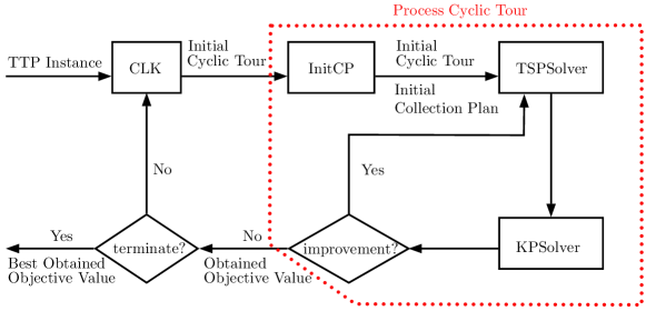
Figure 1: Structure of a typical restart-based cooperative solver for TTP.

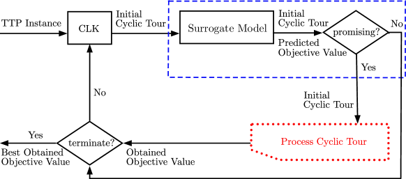
Figure 2: Addition of a surrogate model to the TTP solver in Fig. 1 in order to filter out non-promising initial tours.

3 Proposed Surrogate Model

Using the cooperative strategy shown in Fig. 1, we have empirically observed that for similar initial cyclic tours, the final objective value does not vary much. This suggests that the overall search for a TTP solution with cooperative solvers involves redundant exploration of the solution space. Furthermore, a subset of initial TSP tours (determined during the search) will often lead to poor TTP solutions.

Considering this semi-deterministic nature of the cooperative solvers, we propose a surrogate model to emulate the set of functionality enclosed in the dotted red rectangle in Fig. 1. The surrogate model is used as shown in Fig. 2 within the blue dashed rectangle. For each generated initial tour, the surrogate model provides an approximation of the final TTP objective value. If the generated initial tour appears non-promising, it is disregarded from further optimisation (ie., filtered out). Otherwise, the generated initial tour is allowed to proceed for further iterative optimisation.

For the surrogate model we propose an adaptive learning approach employing non-linear kernel-based support vector regression (SVR) [14, 15]. While solving of a given TTP instance, the surrogate model transitions between several phases as shown in Fig. 3: initialisation, training, testing, and applying. The phases and transitions between phases are elucidated below.

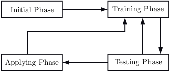
Figure 3: Transitions between phases of the surrogate model.

3.1 Initial Phase

The given TTP instance is solved via restarting for a predefined number of times $t$, where each run uses a new initial tour. For any run $r$ in this phase, the initial tour $c^{r}$ and the corresponding obtained final objective value $g_{r}$ are kept as a pair $\langle c^{r},g_{r}\rangle$ in a training set.

3.2 Training Phase

To aid training the SVR, the training set is first normalised as follows. Considering $g_{\textrm{min}}$ and $g_{\textrm{max}}$ as the minimum and maximum objective values in the training set, each $g_{r}$ is mapped to the [0,1] interval via:

$$n(g_{r})=\dfrac{g_{r}-g_{\textrm{min}}}{g_{\textrm{max}}-g_{\textrm{min}}}$$ (2)

The resulting set $X$=$\{\langle c^{1},n(g_{1})\rangle,\langle c^{2},n(g_{2})\rangle,...,\langle c^{t},n(g_{t})\rangle\}$ is used for training the kernel-based SVR. Given a tour $c$, SVR approximates the normalised final objective value via:

$$n(\widehat{g})=\sum\nolimits_{r=1}^{t}(\alpha_{r}-\alpha_{r}^{*})\cdot k(c^{r},c)+b$$ (3)

where the SVR parameters $b$, $\alpha_{r}$ and $\alpha_{r}^{*}$ for $r\in[1,t]$ are computed as per [14, 15]. For the kernel function $k(c^{a},c^{b})$ we use a customised form of Gaussian radial basis function:

$$k(c^{a},c^{b})=\exp(-\gamma\cdot\Phi(c^{a},c^{b}))$$ (4)

where $\gamma$ is a hyper-parameter, while $\Phi(c^{a},c^{b})$ is a measure of distance between tours $c^{a}$ and $c^{b}$ based on the positions of the cities in the tours:

$$\Phi(c^{a},c^{b})=\dfrac{1}{n}\cdot\sum\nolimits_{j=1}^{n}\dfrac{|c^{a}(j)-c^{b}(j)|}{n-1}$$ (5)

Here, $c(j)$ indicates the position of city $j$ in cyclic tour $c$, hence $|c^{a}(j)-c^{b}(j)|$ is in the $[0,n-1]$ range. As such, $\Phi(c^{a},c^{b})$ is in the $[0,1]$ range.

The approximate final objective value $\widehat{g}$ is obtained by reversing the normalisation:

$$\widehat{g}=n(\widehat{g})\cdot(g_{\textrm{max}}-g_{\textrm{min}})+g_{\textrm{min}}$$ (6)

3.3 Testing Phase

Here the surrogate model is tested to ensure it has adequate accuracy and is retrained if required. The given TTP instance is further solved using new initial tours for $\lambda\cdot t$ times, where $t$ is the number of instances in the training set and $\lambda$ is empirically selected as $0.20$. In every run $r$, for each generated initial cyclic tour $c$, the actual final objective value $g$ as well as the approximate final objective value $\widehat{g}$ are obtained.

There are two conditions where retraining is triggered using an expanded training set. Let us first define a Normalised Error (NE) measure as:

$$\textrm{NE}=n(g)-n(\widehat{g})$$ (7)

For any run which has $\textrm{NE}>e$, where $e$ is a predefined error limit empirically set to $0.02$, the corresponding initial tour and actual final objective value are kept in a temporary buffer. The temporary buffer is initialised to be empty at each start of the testing phase.

A form of moving cumulative average [8] of squares of all obtained NE values is kept, referred to as mean squared normalised error (MSNE). The MSNE is set to zero at each start of the testing phase. For each run (with $r$ starting at $1$), MSNE is updated using:

$$\textrm{MSNE}^{\textrm{[new]}}=\textrm{MSNE}^{\textrm{[old]}}+\dfrac{\textrm{NE}^{2}-\textrm{MSNE}^{\textrm{[old]}}}{r}$$ (8)

The first condition for retraining is as follows. If a run is encountered that has $g<g_{\textrm{min}}$ or $g>g_{\textrm{max}}$, the corresponding initial tour and final objective value are added to the temporary buffer, followed by incorporating the buffer into the training set and immediately restarting the training phase.

The second condition is as follows. If $\textrm{MSNE}>e$ after processing all $\lambda\cdot t$ initial tours, the temporary buffer is incorporated into the training set and the training phase is restarted.

3.4 Applying Phase

Here the surrogate model is employed for filtering out (disregarding) non-promising initial tours. Retraining may also be triggered in a similar manner to the testing phase.

We define maximum tolerable error (MTE) as:

$$\textrm{MTE}=\beta\cdot\sqrt{\textrm{MSNE}}$$ (9)

where $\beta$ is a hyper-parameter. For a given initial tour $c$, the corresponding approximate normalised final objective value $n(\widehat{g})$ is obtained. If $n(\widehat{g})\geq 1-\textrm{MTE}$, the tour $c$ is allowed to proceed for further iterative optimisation. Otherwise, the tour is filtered out either when $n(\widehat{g})<-\textrm{MTE}$, or with a probability of $\sqrt{1-(n(\widehat{g})+\textrm{MTE})^{2}}$. Fig. 4 shows how the probability of filtering out $c$ is based on the value of $n(\widehat{g})$.

Whenever an initial tour $c$ is not filtered out, the given TTP instance is solved using $c$ and the actual final objective value $g$ is obtained. The corresponding NE is computed as per Eqn. (7), followed by updating MSNE as per Eqn. (8).

Similar to the testing phase, if $\textrm{NE}>e$, the corresponding initial tour and actual final objective value are stored in the temporary buffer initialised in the preceding testing phase. If $g<g_{\textrm{min}}$ or $g>g_{\textrm{max}}$, the corresponding initial tour and final objective value are added to the temporary buffer, followed by incorporating the buffer into the training set and immediately restarting the training phase.

Furthermore, retraining occurs whenever $\textrm{MSNE}>e$ or the number of runs with $\textrm{NE}>e$ exceeds $\frac{1}{2}|X|$, where $|X|$ is the current cardinality of the training set. This approach aims to increase the size of the training set during the early stages of optimisation, while reducing the likelihood of retraining on large sets during later stages.

The rationale behind the probabilistic method to filter out non-promising initial tours is twofold. (1) There is always a chance of under-prediction of the final objective value, especially for (desirable) large final objective values. (2) Not filtering out tours with small predicted final objective values makes the updated MSNE value more accurate over the runs in this phase.

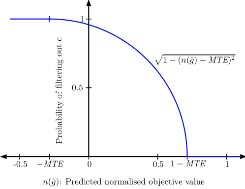
Figure 4: Probability of filtering out tour $c$ based on its approx. normalised final objective value $n(\widehat{g})$.

4 Experiments

As a baseline TTP solver we use the recently proposed cooperative coordination (CoCo) solver [12]. We extend the solver with the proposed surrogate model and refer to it as CoCo-SM.

We use a broad subset of medium and large-sized benchmark TTP instances introduced by [13]. Considered instances are placed into 3 categories. Each category has 32 instances with a range of 574 to 7397 cities. In category A, there is only one item in each city; the profits and weights of the items are strongly correlated; knapsack capacity is relatively small. In category B, there are 5 items in each city; the profits and weights of the items are uncorrelated; the weights of the items are similar to each other; knapsack capacity is moderate. In category C, there are 10 items in each city; the profits and weights of the items are uncorrelated; knapsack capacity is high.

Experiments were performed with $\beta\in\{0,1,2,3\}$ for computing MTE in Eqn. (9). Both solvers were run on each TTP instance 10 times. In each run, CoCo solver was initially run for 1000 restarts on each instance. CoCo-SM was then run on the same instance using the same set of 1000 initial tours generated and used by CoCo for that instance. As such, we can see the effects if the CoCo-SM solver was used instead of the CoCo solver using the same set of the initial tours.

The initial tours and the corresponding actual final objective values in the first 10% of the restarts in each run on each instance were used to build the initial surrogate model in CoCo-SM. For the custom RBF kernel in Eqn. (4), the hyper-parameter $\gamma$ was set to $1$ based on preliminary experiments.

Table 1 shows the results with the configuration of $\beta=2$ in Eqn. (9). The results are presented as the percentage of filtered out tours and the corresponding number of missed best solutions (out of 10 runs). In a “missed best solution”, an initial tour that led to the best possible solution in a run is incorrectly filtered out. The higher the percentage of filtered out tours, the better. The lower number of missed best solutions, the better. The results show that on average about 30% of initial tours are filtered out at the cost of missing about 1 best solution out of 10.

The overhead for training and using the surrogate model is overall negligible. For example, for the hardest to solve instance (the last instance in category C), around 10,000 seconds are required to process 1000 initial tours by the CoCo solver, while about 15 seconds are required to train and use the surrogate model during processing of all the tours in CoCo-SM. As such, if 30% of the initial tours are filtered out, the solver requires about 30% less time to solve a given TTP instance.

Fig. 5 shows the results for $\beta\in\{0,1,2,3\}$ in Eqn. (9), where the the average number of the missed best solutions is plotted against the average percentage of filtered out initial tours. The dashed diagonal line represents the number of expected missed best solutions when random filtering is used instead of filtering based on the surrogate model. As such, better performance is indicated by an operating point that is further away from the diagonal line, moving towards the bottom right corner.

The results indicate that the proposed surrogate model achieves considerably better filtering than simple random filtering. The results also show that there is a trade-off: the larger the percentage of filtered out tours, the higher the chance of missing the best solution.

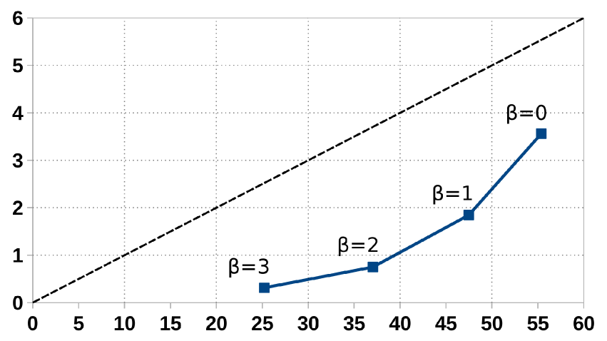
TTP Category A

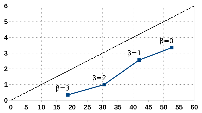
TTP Category B

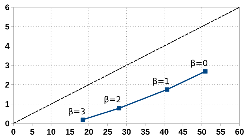
TTP Category C

Figure 5: x-axis: average percentage of the filtered out initial cyclic tours; y-axis: average number of the missed best solutions (out of 10). Each distinct point corresponds to a configuration of $\beta\cdot\sqrt{\textrm{MSNE}}$ as defined in Eqn. (9). The dashed diagonal line represents the number of expected missed best solutions when random filtering is used instead of filtering based on the surrogate model. Better performance is indicated by an operating point that is further away from the diagonal line, moving towards the bottom right corner.

	% of filtered out tours			num. missed best sol.
Instance	A	B	C	A	B	C
u574	36.7	42.8	33.5	0	0	0
rat575	33.4	32.4	37.7	1	3	1
p654	41.5	25.7	41.0	1	2	3
d657	25.8	31.0	20.9	2	1	0
u724	33.0	31.4	33.7	2	1	1
rat783	53.0	37.4	27.3	0	1	0
dsj1000	88.0	51.4	30.1	0	2	1
pr1002	20.9	55.6	41.1	0	3	4
u1060	36.2	47.0	42.6	0	0	0
vm1084	48.3	39.8	30.5	0	1	0
pcb1173	42.0	30.5	32.7	0	0	0
d1291	25.2	30.8	33.4	0	0	0
rl1304	57.6	41.0	43.9	0	0	0
rl1323	51.6	33.9	40.1	0	1	1
nrw1379	30.8	14.8	13.6	1	0	0
fl1400	41.9	56.6	58.3	0	2	0
u1432	26.7	14.8	10.6	1	1	2
fl1577	43.5	30.7	29.5	1	0	0
d1655	41.4	22.5	24.2	2	0	0
vm1748	27.9	41.3	33.9	0	0	2
u1817	38.8	13.6	6.2	2	0	0
rl1889	39.1	22.6	28.3	0	0	2
d2103	44.5	57.4	52.0	4	4	1
u2152	25.7	15.4	17.2	0	0	0
u2319	30.4	28.4	23.3	1	4	0
pr2392	40.6	18.1	17.3	0	1	1
pcb3038	26.9	15.6	13.4	1	0	2
fl3795	31.4	13.2	12.5	0	0	0
fnl4461	20.9	11.6	6.1	3	1	0
rl5915	25.8	24.9	18.7	1	2	2
rl5934	29.7	35.2	30.8	1	1	2
pla7397	26.3	9.9	12.3	0	1	0
Average	37.0	30.5	28.0	0.75	1	0.78

Table 1: Average percentage of the filtered out initial cyclic tours with the corresponding number of missed best solutions (out of 10 runs) using the CoCo-SM solver with the configuration of $\beta=2$ in Eqn. (9). Three categories of TTP instances are used. Category A: knapsack capacity is relatively small; 1 item in each city; weights and profits of items are highly correlated. Category B: knapsack capacity is moderate; 5 items in each city; weights and profits of items are uncorrelated; weights of all items are similar. Category C: knapsack capacity is high; 10 items in each city; weights and profits of items are uncorrelated.

5 Conclusion

We have proposed to increase the efficiency of recent TTP solvers by incorporating a surrogate model that assists in pruning the starting points for restart-based optimisation.

In recent TTP solvers, the solutions to the underlying TSP and KP problems are changed in an iterative and interleaved fashion. The TSP solution (cyclic tour) is typically changed in a deterministic way, while changes to the KP solution typically involve a random search, resulting in a quasi-meandering exploration of the TTP solution space. Upon reaching a plateau, the iterative search of the TTP solution space is restarted by employing a new initial TSP tour.

The proposed surrogate model, based on Support Vector Regression with a novel kernel, adaptively learns the characteristics of initial TSP tours that lead to good TTP solutions. Non-promising initial TSP tours are detected and disregarded, in effect reducing the amount of time spent to find a good TTP solution.

Experiments on benchmark TTP instances show that the proposed approach removes a considerable number of non-promising initial tours, at the cost of missing a small number of the best TTP solutions.

References

- [1] D. Applegate, W. Cook, and A. Rohe. Chained Lin-Kernighan for large traveling salesman problems. INFORMS Journal on Computing, 15(1):82–92, 2003.
- [2] M. J. Asher, B. F. W. Croke, A. J. Jakeman, and L. J. M. Peeters. A review of surrogate models and their application to groundwater modeling. Water Resources Research, 51(8):5957–5973, 2015.
- [3] M. R. Bonyadi, Z. Michalewicz, and L. Barone. The travelling thief problem: The first step in the transition from theoretical problems to realistic problems. In IEEE Congress on Evolutionary Computation (CEC), pages 1037–1044, 2013.
- [4] M. R. Bonyadi, Z. Michalewicz, M. Wagner, and F. Neumann. Evolutionary computation for multicomponent problems: opportunities and future directions. In Optimization in Industry, pages 13–30. Springer, 2019.
- [5] Á. Corberán and G. Laporte. Arc Routing: Problems, Methods, and Applications. SIAM, 2015.
- [6] M. El Yafrani and B. Ahiod. Efficiently solving the Traveling Thief Problem using hill climbing and simulated annealing. Information Sciences, 432:231–244, 2018.
- [7] H. Faulkner, S. Polyakovskiy, T. Schultz, and M. Wagner. Approximate approaches to the traveling thief problem. In Annual Conference on Genetic and Evolutionary Computation, pages 385–392, 2015.
- [8] J. Gama. Knowledge Discovery from Data Streams. Chapman and Hall/CRC, 2010.
- [9] Y. Mei, X. Li, and X. Yao. Improving efficiency of heuristics for the large scale traveling thief problem. In Lecture Notes in Computer Science (LNCS), Vol. 8886, pages 631–643, 2014.
- [10] Z. Michalewicz. Quo vadis, evolutionary computation? In Lecture Notes in Computer Science (LNCS), Vol. 7311, pages 98–121. 2012.
- [11] M. Namazi, M. A. H. Newton, A. Sattar, and C. Sanderson. A profit guided coordination heuristic for travelling thief problems. In Symposium on Combinatorial Search, 2019.
- [12] M. Namazi, C. Sanderson, M. A. H. Newton, and A. Sattar. A cooperative coordination solver for travelling thief problems. arXiv pre-print, 1911.03124, 2019.
- [13] S. Polyakovskiy, M. R. Bonyadi, M. Wagner, Z. Michalewicz, and F. Neumann. A comprehensive benchmark set and heuristics for the traveling thief problem. In Annual Conference on Genetic and Evolutionary Computation, pages 477–484, 2014.
- [14] J. Shawe-Taylor and N. Cristianini. Kernel Methods For Pattern Analysis. Cambridge University Press, 2004.
- [15] A. J. Smola and B. Schölkopf. A tutorial on support vector regression. Statistics and Computing, 14(3):199–222, 2004.