Exactness of SWKB for Shape Invariant Potentials

Abstract

The supersymmetry based semiclassical method (SWKB) is known to produce exact spectra for conventional shape invariant potentials. In this paper we prove that this exactness follows from their additive shape invariance.

keywords: Supersymmetric Quantum Mechanics, Shape Invariance, Exactly Solvable Systems, Semiclassical Approximation, SWKB

I Introduction

The conditions under which semiclassical approximations such as the WKB method yield exact results for quantum-mechanical systems has long been a topic of interest Dunham ; Langer ; Bailey ; Froman ; Krieger1 ; Krieger2 ; Krieger3 ; Bender . In 1985, Comtet et al., in the context of supersymmetric quantum mechanics (SUSYQM), proposed a semiclassical quantization condition Comtet

$$\int_{x_{1}}^{x_{2}}\sqrt{E_{n}-W^{2}(x,a)}\quad{\rm d}x=n\pi\hbar~{},\quad\mbox{where}~{}n=0,1,2,\cdots~{}$$ (1)

that generated exact spectra for several solvable systems. Here $W(x,a)$, the superpotential, is connected to the potential energy given by $V_{-}(x,a)=W^{2}-\hbar/\sqrt{2m}\,\,dW/dx$ and limits ${x_{1}}$ and ${x_{2}}$ are given by $W(x_{i},a)=\pm\sqrt{E_{n}}$. This quantization condition is known as the Supersymmetric WKB method (SWKB). In 1986, Dutt et al. showed that the SWKB condition generated exact spectra for all solvable systems known at that time Dutt . It was later shown that this set comprised all $\hbar$-independent shape invariant superpotentials Bougie2010 ; symmetry .

Even though SWKB quantization has been found on a case-by-case basis Dutt_SUSY to be exact for all $\hbar$-independent shape invariant potentials, there was no general underlying principle to explain it. It has been conjectured Khare1989 ; Dutt91 , but not proved that shape invariance is the source of this SWKB exactness. In this paper we demonstrate that additive shape invariance is sufficient to prove SWKB exactness for all conventional potentials.

II Supersymmetric Quantum Mechanics

In SUSYQM Witten ; Solomonson ; CooperFreedman ; Cooper-Khare-Sukhatme ; Gangopadhyaya-Mallow-Rasinariu , a hamiltonian is written as a product of two differential operators, ${\cal A}^{\pm}=\mp\,\frac{\hbar}{2m}\frac{d}{dx}+W(x,a)$ that are hermitian conjugates of each other. Setting $2m=1$, the product ${\cal A}^{+}\!\cdot{\cal A}^{-}$ generates the hamiltonian

$$H_{-}={\cal A}^{+}\!\cdot{\cal A}^{-}=\left(-\hbar\frac{d}{dx}+W(x,a)\right)\,\left(\hbar\frac{d}{dx}+W(x,a)\right)=-\hbar^{2}\frac{d^{2}}{dx^{2}}+V_{-}(x,a)~{},$$ (2)

where the potential $V_{-}(x,a)$ is given by

$$V_{-}(x,a)=W^{2}(x,a)-\hbar\frac{dW}{dx}.$$ (3)

The function $W(x,a)$ is known as the superpotential of the system. Due to the semi-positive definite nature of the hamiltonian $H_{-}$, its eigenvalues $E^{-}_{n}$ are either positive or zero. If the lowest eigenvalue $E^{-}_{0}\neq 0$, the system is said to have broken supersymmetry. Several authors suggested a modified version of SWKB quantization for systems with broken supersymmetry Eckhardt ; Inomata1 ; Inomata2 . We will assume that our system has unbroken supersymmetry; i.e., the lowest eigenvalue is zero.

The product ${\cal A}^{-}\!\cdot{\cal A}^{+}$ generates another hamiltonian $H_{+}=-\hbar^{2}\frac{d^{2}}{dx^{2}}+V_{+}(x,a)$ with $V_{+}(x,a)=W^{2}(x,a)+\hbar\frac{d\,W}{dx}$. The two hamiltonians are related: ${\cal A}^{+}\!\cdot H_{+}=H_{-}\!\cdot{\cal A}^{+}$ and ${\cal A}^{-}\!\cdot H_{-}=H_{+}\!\cdot{\cal A}^{-}$. These intertwinings lead to the following relationships among the eigenvalues and eigenfunctions of these “partner” hamiltonians:

$$E^{-}_{n+1}=E^{+}_{n},\quad\mbox{where}~{}n=0,1,2,\cdots~{}$$ (4)

$$\frac{~{}~{}~{}{\cal A}^{-}}{\sqrt{E^{+}_{n}}}~{}\psi^{(-)}_{n+1}=~{}\psi^{(+)}_{n}~{}~{}{\rm and}~{}~{}\frac{~{}~{}~{}{\cal A}^{+}}{\sqrt{E^{+}_{n}}}~{}\psi^{(+)}_{n}=~{}\psi^{(-)}_{n+1}~{}.$$ (5)

Thus, knowledge of the eigenvalues and eigenfunctions of one of the hamiltonians automatically gives us their counterparts for the partner hamiltonian. We note that the hamiltonians $H_{\pm}$ remain invariant under the following transformations: $W\rightarrow-W$ and $x\rightarrow-x$. Later in this paper we make use of this property in order to choose signs for some parameters or functions.

II.1 Shape Invariance

If the superpotential $W(x,a_{i})$ obeys the “shape invariance condition” Infeld ; Miller ; gendenshtein1 ; gendenshtein2 ,

$$W^{2}(x,a_{i})+\hbar\frac{d\,W(x,a_{i})}{dx}+g(a_{i})=W^{2}(x,a_{i+1})-\hbar\frac{d\,W(x,a_{i+1})}{dx}+g(a_{i+1}),~{}$$ (6)

the spectra for $H_{-}$ and $H_{+}$ can be determined algebraically. The eigenvalues and eigenfunctions of $H_{-}$ are given by

$$E_{n}^{(-)}(a_{0}) = g(a_{n})-g(a_{0}),$$ (7)

$$\psi^{(-)}_{n}(x,a_{0} )= \frac{{\cal A}^{+}{(a_{0})}~{}{\cal A}^{+}{(a_{1})}\cdots{\cal A}^{+}{(a_{n-1})}}{\sqrt{E_{n}^{(-)}(a_{0})\,E_{n-1}^{(-)}(a_{1})\cdots E_{1}^{(-)}(a_{n-1})}}~{}\psi^{(-)}_{0}(x,a_{n})~{},$$ (8)

where $\psi^{(-)}_{0}(x,a_{n})=Ne^{-\frac{1}{\hbar}\,\int^{x}W(y,a_{n})\,dy}$ is the solution of ${\cal A}^{-}\psi^{(-)}_{0}=0$; i.e., it is the ground-state wavefunction for the eigenvalue $E^{(-)}_{0}=0$, and $N$ is the normalization constant.

In this paper we consider only the case of additive shape invariance: $a_{i+1}=a_{i}+\hbar$. We further restrict our analysis to the superpotentials $W(x,a_{i})$ that have no explicit $\hbar$-dependence; i.e., the $\hbar$-dependence comes in only through parameters $a_{i}$. In Ref. Bougie2010 ; symmetry , the authors showed that in this case, the shape invariance condition reduces to the following two partial differential equations

$$W\,\frac{\partial W}{\partial a}-\frac{\partial W}{\partial x}+\frac{1}{2}\,\frac{dg(a)}{da}=0~{},$$ (9)

$$\frac{\partial^{3}}{\partial a^{2}\partial x}~{}W(x,a)=0~{},$$ (10)

and thus demonstrated that Ref. Dutt_SUSY provided the complete list of such superpotentials, which we called “conventional”. Additional shape invariant superpotentials were later found Quesne1 ; Quesne2 ; Quesne2012a ; Quesne2012b ; Odake1 ; Odake2 ; Tanaka ; Odake3 ; Odake4 ; Ranjani1 , but those were shown to depend explicitly on $\hbar$.

In this paper, we establish that Eqs. (9) and (10) lead to the exactness of SWKB for all conventional superpotentials.

II.2 Three Classes of Conventional Shape Invariant Superpotentials

To prove SWKB exactness from the shape invariance condition for conventional superpotentials, we begin by classifying these superpotentials based on their mathematical form. From Eq. (10), the general form of all such superpotentials is Bougie2010 ; symmetry

$$W(x,a)=a\,f_{1}(x)+f_{2}(x)+u(a)~{}.$$ (11)

This form of a typical conventional superpotential derived from Eq. (10) was conjectured by Infeld et al. Infeld , and examined by others Ramos99 ; Ramos00 . Note that $f_{1}(x)$ and $f_{2}(x)$ cannot both be constant, or $W$ would yield trivial potentials with no $x-$dependence. The following three classes of superpotential comprise all possible forms for $W$. Class I: $f_{1}=\mu$, a constant; Class II: $f_{2}=\mu$, a constant; Class III: $f_{1}$ and $f_{2}$ both have nonzero $x-$dependence. For each class we now determine the properties which follow from additive shape-invariance.

II.2.1 Properties of Class I:

For Class I, $f_{1}=\mu$, a constant. In this case, $W(x,a)=\mu\,a+f_{2}(x)+u(a)$. We can regroup terms by defining $\tilde{u}(a)\equiv u(a)+\mu~{}a$, so that $W(x,a)=f_{2}(x)+\tilde{u}(a)$. Renaming $\tilde{u}$ back to $u$, eq.(9) yields $f_{2}~{}\dot{u}-f_{2}^{\prime}=-\frac{1}{2}\dot{g}-\dot{u}~{}u$, where dots denote derivatives with respect to $a$ and primes denote derivatives with respect to $x$. The RHS is independent of $x$. Since $f_{2}$ does not depend on $a$ and cannot be a constant, each side of the equation is equal to a constant, which we call $\epsilon$. Consequently $\dot{u}=\alpha$, so $u=\alpha~{}a+\beta$ for constants $\alpha$ and $\beta$. Finally, we can regroup terms one more time, such that $\tilde{f_{2}}(x)\equiv f_{2}(x)+\beta$ and $\tilde{\epsilon}\equiv\epsilon+\alpha\beta,$ and then rename $\tilde{f_{2}}$ back to $f_{2}$ and $\tilde{\epsilon}$ back to $\epsilon$.

Therefore, Class I superpotentials can be written as $W(x,a)=f_{2}(x)+\alpha~{}a$, where $\alpha f_{2}-f_{2}^{\prime}=\epsilon$ for constants $\alpha$ and $\epsilon$.

II.2.2 Properties of Class II:

For Class II, $f_{2}=\mu$, a constant. In this case, $W(x,a)=a~{}f_{1}(x)+\mu+u(a)$. We regroup terms such that $u(a)+\mu\rightarrow u(a)$, so that $W(x,a)=a~{}f_{1}(x)+u(a)$. Then Eq.(9) requires $a\left(f_{1}^{2}-f_{1}^{\prime}\right)+f_{1}\left(u+a\dot{u}\right)=-\frac{1}{2}\dot{g}-\dot{u}~{}u$. Since $f_{1}$ is not constant and the right hand side is $x$-independent, this requires $u+a\dot{u}=a~{}\alpha$, so $u=\alpha a/2+B/a$ for constants $B$ and $\alpha$. Similar to Class I, we can shift $f_{1}$ by the constant $\alpha/2$ to absorb the $\alpha a/2$ term into $af_{1}$.

Therefore, Class II superpotentials can be written as $W(x,a)=af_{1}(x)+B/a$, where $f_{1}^{2}-f_{1}^{\prime}=\lambda$ for constants $B$ and $\lambda$.

II.2.3 Properties of Class III:

For Class III, neither $f_{1}$ nor $f_{2}$ is constant. We first note that if $f_{2}$ is of the form $f_{2}(x)=\nu f_{1}(x)+\mu$ for any constants $\mu$ and $\nu$, then with a redefinition of $a\to a+\nu$, $W$ can be considered equivalent to a Class II superpotential in which $f_{2}$ is a constant. Similarly, if $u(a)$ is linear in $a$, this is equivalent to the case $u(a)=0$ by regrouping terms.

With these assumptions, we substitute the form of $W$ from Eq.(11) in Eq. (9) and get

$$-a\left(f_{1}^{2}-f_{1}^{\prime}\right)+\left(f_{2}^{\prime}-f_{1}f_{2}\right)-f_{1}\left(u+a\dot{u}\right)-\dot{u}f_{2}=g/2+\dot{u}u~{}.$$ (12)

The first two terms in this equation are respectively linear in $a$ and independent of $a$. Therefore, if there is any nonlinearity in $a$ on the right hand side of the equation, it could only come from the third and fourth terms of the left hand side. However, the right hand side of this equation is independent of $x$; since $f_{1}$ and $f_{2}$ are not constant and are linearly independent, the $x$-dependence in the third term cannot be canceled by the fourth term, and vice versa. Consequently, the coefficients of $f_{1}$ and $f_{2}$ in terms three and four must each be linear functions of $a$.

Linearity in $a$ of the $\dot{u}f_{2}$ term in Eq. (12) implies $u=\mu a^{2}/2+\nu a+\gamma$. Then $u+a\dot{u}=3\mu a^{2}/2+2\nu a+\gamma$, which is linear in $a$ only if $\mu=0$. Thus $u$ itself is linear in $a$, so we can set $u=0$. We then have $-a\left(f_{1}^{2}-f_{1}^{\prime}\right)+\left(f_{2}^{\prime}-f_{1}f_{2}\right)=g/2+\dot{u}u$. Since the right-hand-side is independent of $x$, this requires $f_{1}^{2}-f_{1}^{\prime}=\lambda$ and $f_{1}f_{2}-f_{2}^{\prime}=\varepsilon$ for constants $\lambda$ and $\varepsilon$.

Therefore, Class III superpotentials can be written as $W(x,a)=af_{1}(x)+f_{2}(x)$, where $f_{1}^{2}-f_{1}^{\prime}=\lambda$ and $f_{1}f_{2}-f_{2}^{\prime}=\varepsilon$ for constants $\lambda$ and $\varepsilon$.

III Exactness of SWKB

In this section we will show that for the three classes defined above, the definite integral of Eq. (1) is $n\pi\hbar$. Let us define a function $I(a,n,\hbar)$ by

$$I(a,n,\hbar)\equiv\int_{x_{1}}^{x_{2}}\sqrt{E_{n}-W^{2}(x,a)}\quad{\rm d}x~{}.$$ (13)

Since $W(x,a)$ does not depend on $\hbar$, the energy $E_{n}=g(a+n\hbar)-g(a)$ is the sole source of $n$ and $\hbar$ dependence of the integrand ${\cal F}(x)=\sqrt{E_{n}-W^{2}(x,a)}$. We will prove that $I(a,n,\hbar)=n\pi\hbar$.

First, we note that for $n=0$, $E_{0}=0$. Hence, ${x_{1}}$ and ${x_{2}}$, the roots of $W(x)=\pm\sqrt{E_{n}}$, are equal, so $I(a,0,\hbar)=0$. Thus Eq. (1) holds for $n=0$.

Second, we observe that for all finite values of $a$ and $n$, $\lim_{\hbar\rightarrow 0}E_{n}\rightarrow 0$. Thus for all $n$, $I(a,n,0)=0$, so if we Taylor expand $I(a,n,\hbar)$ in powers of $\hbar$, there would be no $\hbar$-independent term. I.e.,

$$I(a,n,\hbar)=\sum_{k=1}^{\infty}c_{k}(a,n)\,\hbar^{k}~{}.$$ (14)

We now compute the first derivative $\frac{\partial I(a,n,\hbar)}{\partial\hbar}$ for any value of $n$:

$$\frac{\partial I(a,n,\hbar)}{\partial\hbar}=\frac{\partial x_{2}}{\partial\hbar}{\cal F}(x_{2})-\frac{\partial x_{1}}{\partial\hbar}{\cal F}(x_{1})+\frac{1}{2}\frac{\partial E_{n}}{\partial\hbar}\int_{x_{1}}^{x_{2}}\frac{{\rm d}x}{\sqrt{E_{n}-W^{2}(x,a)}\quad}.$$ (15)

Integrating it, we will determine $I(a,n,\hbar)$. Since ${\cal F}(x)$ vanishes at points ${x_{1}}$ and ${x_{2}}$,

$$\frac{\partial I(a,n,\hbar)}{\partial\hbar}=\frac{1}{2}\frac{\partial E_{n}}{\partial\hbar}\int_{x_{1}}^{x_{2}}\frac{{\rm d}x}{\sqrt{E_{n}-W^{2}(x,a)}\quad}~{},$$ (16)

which is the starting point for proof of SWKB exactness for conventional superpotentials.

Note that if $W(x,a)$ were to have an intrinsic dependence on $\hbar$, as is the case for the extended superpotentials Quesne1 ; Quesne2 ; Quesne2012a ; Quesne2012b ; Odake1 ; Odake2 ; Tanaka ; Odake3 ; Odake4 , Eq. (10) would not hold and $W$ would not be restricted to the three classes above, which subsume all the conventional superpotentials. In this case we would have an extra term in Eq. (15). Thus, $\hbar$-dependence of $W$ could impact the exactness of SWKB. For example, a numerical computation Bougie2017 showed that SWKB was not exact for the extension of the 3D-Oscillator Quesne1 .

Next, we will prove that $\partial I(a,n,\hbar)/\partial\hbar=n\pi$, hence $I(a,n,\hbar)=n\pi\hbar$ for the three classes enumerated in Sec.II.2.

III.1 Class I

For this class, we found in Sec.II.2 that $W(x,a)=f_{2}(x)+\alpha~{}a$, where $\alpha f_{2}-f_{2}^{\prime}=\epsilon$ for constants $\alpha$ and $\epsilon$. We consider two cases in this class, $\alpha=0$ and $\alpha\neq 0$.

III.1.1 Class IA: $\alpha=0$

In this case, $W(x,a)=f_{2}(x)$, where $W^{\prime}(x)=f_{2}^{\prime}(x)=-\varepsilon$. From Eq. 9 $dg/da=-2\varepsilon$. To avoid level crossing, $dg/da$ must be positive. We define $\omega\equiv-2\varepsilon>0$, so $dg/da=\omega$, $E_{n}=n\omega\hbar$, therefore $\partial E_{n}/\partial\hbar=n\omega$. We now solve Eq. 16 with these values:

$$\frac{\partial I(a,n,\hbar)}{\partial\hbar}=\frac{n\omega}{2}\int_{x_{1}}^{x_{2}}\frac{{\rm d}x}{\sqrt{E_{n}-W^{2}(x)}},$$

where $x_{1}$ and $x_{2}$ are given by solutions to $E_{n}-W^{2}=0$. We change the integration variable to obtain

$$\frac{\partial I(a,n,\hbar)}{\partial\hbar}=\frac{n\omega}{2}\int_{-\sqrt{E_{n}}}^{\sqrt{E_{n}}}\frac{2dW}{\omega\sqrt{E_{n}-W^{2}(x)}}=n\int_{-\sqrt{E_{n}}}^{\sqrt{E_{n}}}\frac{dW}{\sqrt{E_{n}-W^{2}(x)}}=n\pi.$$

III.1.2 Class IB: $\alpha\neq 0$

In this case, $W(x,a)=f_{2}(x)+\alpha\,a$, where $\alpha f_{2}-f_{2}^{\prime}=\epsilon$ for nonzero $\alpha$. With a redefinition $a+\varepsilon/\alpha\rightarrow a$, we can set $\varepsilon=0$ and $f_{2}-\epsilon/\alpha\rightarrow f_{2}$. Thus, we have

$$W(x,a)=\alpha\,a+f_{2}(x)\quad\mbox{and}\quad\frac{\partial W}{\partial x}=f_{2}^{\prime}(x)=\alpha f_{2}(x)=\alpha\,(W-\alpha\,a)~{}.$$ (17)

Since $f_{2}^{\prime}=\alpha f_{2}$, $f_{2}$ cannot be zero at any point, or it would be zero everywhere. Hence $W^{\prime}$ must have a definite sign, which for unbroken supersymmetry must be positive. This implies that $\alpha f_{2}>0$, so $\alpha$ and $f_{2}$ must have the same sign. Without loss of generality , we assume $\alpha<0$; consequently, $f_{2}<0$. From Eq. (9), we have $dg/da=-2\alpha^{2}\,a$. Because $dg/da>0$ we must have $a<0$ (and $a+n\hbar<0$ for all bound states), thus $W<\alpha\,a$. By integrating $g$, we get $E_{n}=g(a+n\hbar)-g(a)=\alpha^{2}\,a^{2}-\alpha^{2}(a+n\hbar)^{2}$. Then

$$\frac{\partial I(a,n,\hbar)}{\partial\hbar}=\frac{1}{2}\frac{\partial E_{n}}{\partial\hbar}\int_{x_{1}}^{x_{2}}\frac{{\rm d}x}{\sqrt{E_{n}-W^{2}(x,a)}}=\frac{1}{2\alpha}\frac{\partial E_{n}}{\partial\hbar}\int_{-\sqrt{E_{n}}}^{\sqrt{E_{n}}}\frac{{\rm d}W}{(W-\alpha\,a)\sqrt{E_{n}-W^{2}(x,a)}}.$$

We carry out the integration in the complex $W$ plane, as shown in Fig. 1.

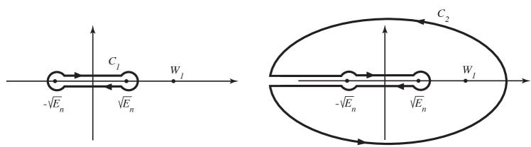
Figure 1: The contour includes one pole at $W_{1}=\alpha\,a$

The contour includes a pole at $W_{1}=\alpha\,a$, and a cut from ${-\sqrt{E_{n}}}$ to ${\sqrt{E_{n}}}$. The partial derivative $\frac{\partial I(a,n,\hbar)}{\partial\hbar}$ is then given by

$$\frac{\partial I(a,n,\hbar)}{\partial\hbar} = \frac{1}{4\alpha}\frac{\partial E_{n}}{\partial\hbar}\oint\frac{{\rm d}W}{(W-\alpha\,a)\sqrt{E_{n}-W^{2}(x,a)}}$$ (18)

$$= \frac{1}{4\alpha}\frac{\partial E_{n}}{\partial\hbar}\frac{2\pi\,i}{\sqrt{E_{n}-\alpha^{2}\,a^{2}}}=\frac{1}{4\alpha}\frac{\partial E_{n}}{\partial\hbar}\frac{2\pi\,i}{\sqrt{-\alpha^{2}(a+n\hbar)^{2}}}$$

$$= \frac{n\pi}{2\alpha^{2}}\,\frac{-2\alpha^{2}(a+n\hbar)}{-(a+n\hbar)}=n\pi~{},$$

where we substituted ${\partial E_{n}}/{\partial\hbar}={-2\alpha^{2}(a+n\hbar)n}$.

III.2 Class II

From Sec.II.2, this class is of the form $W(x,a)=af_{1}(x)+B/a$, where $f_{1}^{2}-f_{1}^{\prime}=\lambda$ for constants $B$ and $\lambda$. From 9, this requires

$$\frac{dg}{da}=\frac{2B^{2}}{a^{3}}-2\lambda\,a;~{}~{}g(a)=-\frac{B^{2}}{a^{2}}-\lambda\,a^{2}~{},$$ (19)

and thus $E_{n}=\frac{B^{2}}{a^{2}}-\frac{B^{2}}{(a+n\hbar)^{2}}+\lambda\left[\,a^{2}-(a+n\hbar)^{2}\right]$. From $dg/da=\frac{2B^{2}}{a^{3}}-2\lambda\,a$, we see that if $\lambda\leq 0$, we must have $a>0$. For $\lambda>0$, we have two cases: $a>0$ and ${B^{2}}>\lambda\,a^{4}$, or $a<0$ and ${B^{2}}<\lambda\,a^{4}$.

Using $W^{\prime}=a(f_{1}^{2}-\lambda)$, we change the integration variable:

$$dx=\frac{a\,dW}{\left(W-B/a\right)^{2}-\lambda\,a^{2}}~{}.$$

Then Eq. (16) becomes

$$\frac{\partial I(a,n,\hbar)}{\partial\hbar}=\frac{a}{2}\frac{\partial E_{n}}{\partial\hbar}\int_{-\sqrt{E_{n}}}^{\sqrt{E_{n}}}\frac{dW}{\left[\left(W-B/a\right)^{2}-\lambda\,a^{2}\right]\sqrt{E_{n}-W^{2}}}~{}.$$ (20)

Here we have two cases: $\lambda=0$ and $\lambda\neq 0$.

III.2.1 Class IIA: $\lambda=0$

For $\lambda=0$, since $f_{1}^{\prime}=f_{1}^{2}$, we see that if $f_{1}=0$, at one point, it must be zero at all points. Hence $f_{1}$ must have a definite sign everywhere. Without loss of generality, we choose $f_{1}<0$. Then, since $W=af_{1}(x)+B/a$ must change sign to preserve supersymmetry, we must have $B>0$. Hence, Eq. (20) becomes

$$\frac{\partial I(a,n,\hbar)}{\partial\hbar}=\frac{anB^{2}}{(a+n\hbar)^{3}}\int_{-\sqrt{E_{n}}}^{\sqrt{E_{n}}}\frac{dW}{\left(W-B/a\right)^{2}\sqrt{E_{n}-W^{2}}}~{}~{},$$ (21)

which integrates to

$$\frac{\partial I(a,n,\hbar)}{\partial\hbar}=\frac{anB^{2}}{(a+n\hbar)^{3}}\frac{a^{2}B\pi}{(B^{2}-a^{2}E_{n})^{3/2}}=n\pi~{},$$ (22)

where we used $E_{n}=\frac{B^{2}}{a^{2}}-\frac{B^{2}}{(a+n\hbar)^{2}}$.

III.2.2 Class IIB: $\lambda\neq 0$

This class splits into two cases: $\lambda>0$ and $\lambda<0$.

We will consider first the case when $\lambda>0$. Because

$$E_{n}=\frac{B^{2}}{a^{2}}-\frac{B^{2}}{(a+n\hbar)^{2}}+\lambda\left[\,a^{2}-(a+n\hbar)^{2}\right]~{},$$ (23)

Eq. (20) becomes

$$\frac{\partial I(a,n,\hbar)}{\partial\hbar}=\frac{a}{2}\left[\frac{2B^{2}n}{(a+n\hbar)^{3}}-2n\lambda(a+n\hbar)\right]\int_{-\sqrt{E_{n}}}^{\sqrt{E_{n}}}\frac{dW}{(W-W_{1})(W-W_{2})\sqrt{E_{n}-W^{2}}}$$ (24)

where the simple poles $W_{1}=B/a+a\sqrt{\lambda}$ and $W_{2}=B/a-a\sqrt{\lambda}$ are both greater than $\sqrt{E_{n}}$ , and $B>\sqrt{\lambda}(a+n\hbar)^{2}$. To compute this integral we first observe that it can be written as a sum of two integrals which can be evaluated independently. Using Eq. (23), we obtain

$$J \equiv\int_{-\sqrt{E_{n}}}^{\sqrt{E_{n}}}\frac{dW}{(W-W_{1})(W-W_{2})\sqrt{E_{n}-W^{2}}}$$

$$=\frac{1}{W_{1}-W_{2}}\int_{-\sqrt{E_{n}}}^{\sqrt{E_{n}}}\frac{dW}{(W-W_{1})\sqrt{E_{n}-W^{2}}}+\frac{1}{W_{2}-W_{1}}\int_{-\sqrt{E_{n}}}^{\sqrt{E_{n}}}\frac{dW}{(W-W_{2})\sqrt{E_{n}-W^{2}}}$$

$$=-\frac{\pi(a+n\hbar)}{2a\sqrt{\lambda}\,\left(B+\sqrt{\lambda}(a+n\hbar)^{2}\right)}+\frac{\pi(a+n\hbar)}{2a\sqrt{\lambda}\left(B-\sqrt{\lambda}\,(a+n\hbar)^{2}\right)}=~{}\frac{\pi(a+n\hbar)^{3}}{aB^{2}-a\lambda(a+n\hbar)^{4}}~{}.$$

Substituting $J$ back into Eq. (24) we arrive at

$$\frac{\partial I(a,n,\hbar)}{\partial\hbar}=n\pi~{}.$$ (25)

Let us now consider the case when $\lambda=-\mu<0$. Then Eq. (20) becomes

$$\frac{\partial I(a,n,\hbar)}{\partial\hbar}=\frac{a}{2}\left[\frac{2B^{2}n}{(a+n\hbar n)^{3}}+2n\mu(a+n\hbar)\right]\int_{-\sqrt{E_{n}}}^{\sqrt{E_{n}}}\frac{dW}{(W-U_{1})(W-U_{2})\sqrt{E_{n}-W^{2}}}~{},$$ (26)

where the simple poles are $U_{1}=B/a+ia\sqrt{\mu}$ and $U_{2}=B/a-ia\sqrt{\mu}$. Note that this is a real positive integral . The complex factorization in Eq. (26) was done in order to carry out the calculations in the complex $W$ plane, as illustrated in Fig. (2). We obtain for the integral in Eq. (26):

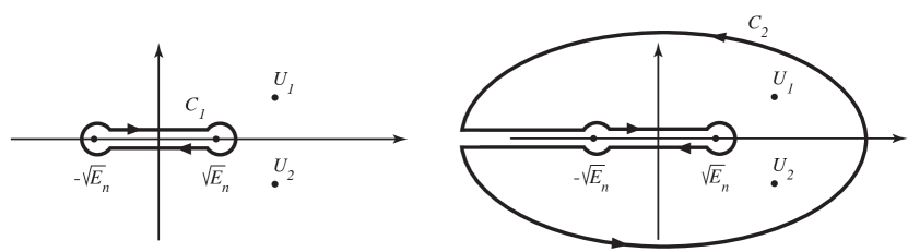
Figure 2: Complex integration for $\lambda=-\mu<0$ case. The contour $C_{2}$ includes simple poles $U_{1}=B/a+ia\sqrt{\mu}$ and $U_{2}=B/a-ia\sqrt{\mu}$.

$$J\equiv \int_{-\sqrt{E_{n}}}^{\sqrt{E_{n}}}\frac{dW}{(W-U_{1})(W-U_{2})\sqrt{E_{n}-W^{2}}}$$

$$= \frac{\pi(a+n\hbar)}{2a\sqrt{\mu}}\left(\frac{1}{\sqrt{\left(\sqrt{\mu}(a+n\hbar)^{2}-iB\right)^{2}}}-\frac{1}{\sqrt{\left(\sqrt{\mu}(a+n\hbar)^{2}+iB\right)^{2}}}\right)$$

$$= \frac{\pi(a+n\hbar)}{2a\sqrt{\mu}}\left(\frac{e_{1}}{{\sqrt{\mu}(a+n\hbar)^{2}-iB}}-\frac{e_{2}}{{\sqrt{\mu}(a+n\hbar)^{2}+iB}}\right)~{},$$ (27)

where $e_{1},e_{2}=\pm 1$. When substituted into Eq. (26), this gives

$$\frac{\partial I(a,n,\hbar)}{\partial\hbar}=\frac{1}{2}\pi n\left(e_{1}-e_{2}+\frac{iB(e_{1}+e_{2})}{\sqrt{\mu}(a+n\hbar)^{2}}\right)~{}.$$ (28)

Since this is a real positive integral, we must have $e_{1}+e_{2}=0$ and $e_{1}=1$. We arrive at

$$\frac{\partial I(a,n,\hbar)}{\partial\hbar}=n\pi~{}.$$ (29)

III.3 Class III

For Class III, $W(x,a)=af_{1}(x)+f_{2}(x)$, where $f_{1}^{2}-f_{1}^{\prime}=\lambda$ and $f_{1}f_{2}-f_{2}^{\prime}=\varepsilon$, for constants $\lambda$ and $\varepsilon$. We have two cases in this class, $\lambda=0$ and $\lambda\neq 0$. We now examine each case separately.

III.3.1 Class IIIa: $\lambda=0$

In this case, $f_{1}^{\prime}=f_{1}^{2}$, hence $f_{1}$ cannot be zero at any point. Also, $f_{2}^{\prime}=f_{1}\,f_{2}-\varepsilon$. The homogeneous equation for $f_{2}^{\prime}=f_{1}\,f_{2}-\varepsilon$ is solved by $f_{2}=\alpha f_{1}$. A particular solution is $f_{2}=\frac{1}{2}\varepsilon/f_{1}$. Thus, the superpotential takes the form $W=af_{1}+\alpha f_{1}+\frac{1}{2}\varepsilon/f_{1}=(a+\alpha)f_{1}+\frac{1}{2}\varepsilon/f_{1}\equiv af_{1}+\frac{1}{2}\varepsilon/f_{1}$, where we have redefined the parameter $a$. From Eq. 9, $dg/da=-2\varepsilon>0$, implies $\varepsilon<0$, which requires that $W^{\prime}=af_{1}^{2}-\varepsilon/2>0$, because $a>0$. So

$$\frac{\partial I(a,n,\hbar)}{\partial\hbar} = \frac{1}{2}\frac{\partial E_{n}}{\partial\hbar}\int_{x_{1}}^{x_{2}}\frac{dx}{\sqrt{E_{n}-\left(af_{1}+\frac{1}{2}\varepsilon/f_{1}\right)^{2}}}~{}.$$

Changing the integration variable to $f_{1}$,

$$\frac{\partial I(a,n,\hbar)}{\partial\hbar} = \frac{1}{2}\frac{\partial E_{n}}{\partial\hbar}\int_{f_{L}}^{f_{R}}\frac{df_{1}}{f_{1}^{2}\sqrt{E_{n}-\left(af_{1}+\frac{1}{2}\varepsilon/f_{1}\right)^{2}}},$$

where ${f_{L}}$ and ${f_{R}}$ are the turning points on the $f_{1}$ axis, where the square root in the denominator is zero. Moving to the complex $f_{1}$-plane,

$$\frac{\partial I(a,n,\hbar)}{\partial\hbar} = \frac{1}{2}\frac{1}{2}\frac{\partial E_{n}}{\partial\hbar}\oint\frac{df_{1}}{f_{1}^{2}\sqrt{E_{n}-\left(af_{1}+\frac{1}{2}\varepsilon/f_{1}\right)^{2}}}$$

$$= \frac{1}{4}{\frac{1}{2}\,(-2\varepsilon)\,}n\oint\frac{df_{1}^{2}}{f_{1}^{2}\sqrt{E_{n}f_{1}^{2}-\left(af_{1}^{2}+\frac{1}{2}\varepsilon\right)^{2}}}=-\frac{1}{4}\varepsilon n(2\pi i)\frac{2}{-i\,\epsilon}=n\pi.$$

III.3.2 Class IIIb: $\lambda\neq 0$

In this case, $f_{1}^{\prime}=f_{1}^{2}-\lambda$, $f_{2}^{\prime}=f_{1}\,f_{2}-\varepsilon$, and $W=af_{1}+f_{2}$. The homogeneous and particular solutions for $f_{2}$ are $\beta\sqrt{f_{1}^{2}-\lambda}$ and $f_{1}\left(\frac{\varepsilon}{\lambda}\right)$ respectively . Thus, with a redefinition of the parameter $a$, we get $W=af_{1}+f_{1}\left(\frac{\varepsilon}{\lambda}\right)+\beta\sqrt{f_{1}^{2}-\lambda}=\left(a+\frac{\varepsilon}{\lambda}\right)\,f_{1}+\beta\sqrt{f_{1}^{2}-\lambda}\equiv af_{1}+\beta\sqrt{f_{1}^{2}-\lambda}$.

From Eq. 9 we have $g(a)=-\lambda\,a^{2}$, so $E_{n}=\lambda\left[a^{2}-(a+n\hbar)^{2}\right]$, and $\partial E_{n}/\partial\hbar=-2n\lambda(a+n\hbar)$. To ensure the order $E_{n+1}>E_{n}>E_{n-1}$, we must have $\lambda(a+n\hbar)<0$.

Using the fact that $f_{1}^{2}\neq\lambda$, we define a function $y(x)\equiv\frac{\sqrt{\lambda}-f_{1}}{\sqrt{\lambda}+f_{1}}$. Its derivative is given by $\frac{dy}{dx}=2\sqrt{\lambda}y$, which yields $f_{1}=\sqrt{\lambda}\left(\frac{y-1}{y+1}\right)$. We now define two functions ${\cal{S}}(x)\equiv\frac{y^{1/2}-y^{-1/2}}{2\sqrt{\lambda}}$, and ${\cal{C}}(x)\equiv\frac{y^{1/2}+y^{-1/2}}{2}$, which satisfy the identities:

$$\begin{array}[]{lll}{d{\cal{C}}}/{dx}=\lambda{\cal{S}}~{},&{d{\cal{S}}}/{dx}={\cal{C}}~{},&{\cal{C}}^{2}(y)-\lambda\,{\cal{S}}^{2}(y)=1~{},\\ 2\,{\cal{C}}(y)\,{\cal{S}}(y)={\cal{S}}(y^{2})~{},&{\cal{C}}^{2}(y)+\lambda\,{\cal{S}}^{2}(y)={\cal{C}}(y^{2})~{}.\end{array}$$

In terms of these variables, $f_{1}=-\lambda\frac{{\cal{S}}}{{\cal{C}}}$ and $f_{2}=\beta\sqrt{f_{1}^{2}-\lambda}=\frac{\beta}{{\cal{C}}}$, where $\beta$ is a constant. Now, we proceed to compute ${\partial I(a,n,\hbar)}/{\partial\hbar}$ for this case.

$$\frac{\partial I(a,n,\hbar)}{\partial\hbar} = \frac{1}{2}\frac{\partial E_{n}}{\partial\hbar}\int_{x_{1}}^{x_{2}}\frac{dx}{\sqrt{E_{n}-W^{2}}}~{}=~{}-n\lambda(a+n\hbar)\int_{x_{1}}^{x_{2}}\frac{dx}{\sqrt{E_{n}-(af_{1}+f_{2})^{2}}}~{},$$

which can be written as

$$\frac{\partial I(a,n,\hbar)}{\partial\hbar} = -n\lambda(a+n\hbar)\int_{x_{1}}^{x_{2}}\frac{dx}{\sqrt{E_{n}-(-\frac{\lambda{\cal{S}}a}{{\cal{C}}}+\frac{\beta}{{\cal{C}}})^{2}}}$$ (30)

$$= -\frac{1}{2}\,n\lambda(a+n\hbar)\oint\frac{d{\cal{S}}}{\sqrt{E_{n}\,\left(1+\lambda{\cal{S}}^{2}\right)-\lambda^{2}a^{2}{\cal{S}}^{2}+2\lambda{\cal{S}}\beta a-\beta^{2}}}$$

$$= -\frac{1}{2}\,n\lambda(a+n\hbar)\oint\frac{d{\cal{S}}}{\sqrt{{\cal{S}}^{2}\left(\lambda E_{n}-\lambda^{2}a^{2}\right)+2\lambda{\cal{S}}\beta a-\beta^{2}}}$$

$$= -\frac{1}{2}\,n\lambda(a+n\hbar)\oint\frac{dt}{t\sqrt{\left(\lambda E_{n}-\lambda^{2}a^{2}\right)+2\lambda\beta a\,t-\beta^{2}t^{2}}},\quad\quad\mbox{where }t\equiv 1/{\cal{S}}\,;$$

$$= -\frac{1}{2}\,n\lambda(a+n\hbar)\,\frac{2\pi i}{\sqrt{-\lambda^{2}(a+n\hbar)^{2}}}\,=-\frac{1}{2}\,n\,\frac{2\pi(a+n\hbar)}{\left|a+n\hbar\right|}\,=n\pi~{},$$

where we have used the constraint $\lambda(a+n\hbar)<0$.

IV Conclusion

In this paper we have proved that the exactness of SWKB for conventional superpotentials follows from the additive shape invariance condition.

References

• (1) J. Dunham, The WKB Method of Solving the Wave Equation; Phys.Rev. 41 (1932) 721.
• (2) R. E. Langer, On the Connection Formulas and the Solutions of the Wave Equation; Phys. Rev. 51, (1937) 669–676.
• (3) P. B. Bailey, Exact Quantization Rules for the One‐Dimensional Schrödinger Equation with Turning Points; Jour. of Math. Phys. 5, 1293 (1964).
• (4) N. Froman and P. O. Froman, JWKB Approximation; Contributions to the Theory; (North-Holland Publ. Co., Amsterdam, 1965).
• (5) J. B. Krieger, M. L. Lewis, and C. Rosenzweig, Use of the WKB Method for Obtaining Energy Eigenvalues; J. Chem. Phys. 47, 2942 (1967).
• (6) C. Rosenzweig, and J. B. Krieger, Exact Quantization Conditions; Jour. of Math. Phys. 9, 849 (1968);
• (7) J. B. Krieger, Exact Quantization Conditions II; Jour. of Math. Phys. 10, 1455 (1969).
• (8) Carl M. Bender, Kaare Olaussen, and Paul S. Wang, Numerological analysis of the WKB approximation in large order; Phys. Rev. D 16, (1977) 1740–1748.
• (9) A. Comtet, A.D. Bandrauk and D.K. Campbell, Exactness of Semiclassical Bound State Energies for Supersymmetric Quantum Mechanics; Phys.Lett. 150B (1985) 159–162.
• (10) R. Dutt, A. Khare, U. Sukhatme, Exactness of Supersymmetry WKB Spectra for Shape-Invariant Potentials; Phys.Lett. 181B (1986) 295–298.
• (11) J. Bougie, A. Gangopadhyaya, J. V. Mallow, Generation of a complete set of additive shape-invariant potentials from an Euler equation; Phys. Rev. Lett. (2010) 210402:1–210402:4.
• (12) J. Bougie, A. Gangopadhyaya, J. V. Mallow, C. Rasinariu, Supersymmetric quantum mechanics and solvable models; Symmetry 4 (3) (2012) 452–473.
• (13) R. Dutt, A. Khare, U. Sukhatme, Supersymmetry, shape invariance and exactly solvable potentials; Am. J. Phys. 56 (1988) 163–168.
• (14) A. Khare, Y. P. Varshni, Is shape invariance also necessary for the lowest order supersymmetric WKB to be exact?; Phys. Lett. A 142A (1989) 1–4. https://doi.org/10.1016/0375-9601(89)90701-9.
• (15) R. Dutt, A. Khare, U. Sukhatme, Supersymmetry‐inspired WKB approximation in quantum mechanics; Am. Jour Phys., 59, 723 (1991); https://doi.org/10.1119/1.16840
• (16) E. Witten, Dynamical breaking of supersymmetry; Nucl. Phys. B185 (1981) 513–554.
• (17) P. Solomonson, J. W. Van Holten, Fermionic coordinates and supersymmetry in quantum mechanics; Nucl. Phys. B196 (1982) 509–531.
• (18) F. Cooper, B. Freedman, Aspects of supersymmetric quantum mechanics; Ann. Phys. 146 (1983) 262–288.
• (19) F. Cooper, A. Khare, U. Sukhatme, Supersymmetry in Quantum Mechanics, World Scientific, Singapore, 2001.
• (20) A. Gangopadhyaya, J. Mallow, C. Rasinariu, Supersymmetric Quantum Mechanics: An Introduction (2nd ed.), World Scientific, Singapore, 2017.
• (21) B. Eckhardt, Maslov-WKB theory for supersymmetric hamiltonians; Phys. Lett. B 168 (1986) 245-7. https://doi.org/10.1016/0370-2693(86)90972-X
• (22) A. Inomata and G. Junker, Quasiclassical approach to the path-integrals in supersymmetric quantum mechanics; Lectures on Path Integration: Trieste 1991, ed. H. A. Cerdeira, S. Lundqvist, D. Mugnai, A. Ranfagni, V. Sa-yakanit and L. S. Schulman (Singapore: World Scientific) pp 460-482.
• (23) A. Inomata and G. Junker, Quasiclassical path-integral approach to supersymmetric quantum mechanics; Phys. Rev. A 50, (1994) 3638–3649.
• (24) L. Infeld, T. E. Hull, The factorization method; Rev. Mod. Phys. 23 (1951) 21–68.
• (25) W. Miller Jr, Lie Theory and Special Functions (Mathematics in Science and Engineering); Academic Press, New York, NY, USA, 1968.
• (26) L. E. Gendenshtein, Derivation of exact spectra of the Schrödinger equation by means of supersymmetry; JETP Lett. 38 (1983) 356–359.
• (27) L. E. Gendenshtein, I. V. Krive, Supersymmetry in quantum mechanics; Sov. Phys.Usp. 28 (1985) 645–666.
• (28) C. Quesne, Exceptional orthogonal polynomials, exactly solvable potentials and supersymmetry; J. Phys. A 41 (2008) 392001:1–392001:6.
• (29) C. Quesne, Solvable rational potentials and exceptional orthogonal polynomials in supersymmetric quantum mechanics; Sigma 5 (2009) 084:1–084:24.
• (30) C. Quesne, Novel enlarged shape invariance property and exactly solvable rational extensions of the Rosen-Morse II and Eckart potentials; Sigma 8 (2012) 080.
• (31) C. Quesne, Revisiting (quasi-)exactly solvable rational extensions of the Morse potential; Int. J. Mod. Phys. A 27 (2012) 1250073.
• (32) S. Odake, R. Sasaki, Infinitely many shape invariant discrete quantum mechanical systems and new exceptional orthogonal polynomials related to the Wilson and Askey-Wilson polynomials; Phys. Lett. B 682 (2009) 130–136.
• (33) S. Odake, R. Sasaki, Another set of infinitely many exceptional $(x_{\ell})$ Laguerre polynomials; Phys. Lett. B 684 (2010) 173–176.
• (34) T. Tanaka, N-fold supersymmetry and quasi-solvability associated with x-2-Laguerre polynomials; J. Math. Phys. 51 (2010) 032101:1–032101:20.
• (35) S. Odake, R. Sasaki, Exactly solvable quantum mechanics and infinite families of multi-indexed orthogonal polynomials; Phys. Lett. B 702 (2011) 164–170.
• (36) R. Odake, S.and Sasaki, Extensions of solvable potentials with finitely many discrete eigenstates; J. Phys. A 46 (2013) 235–205.
• (37) S. Sree Ranjani, P. K. Panigrahi, A. K. Kapoor, A. Khare, A. Gangopadhyaya, Exceptional orthogonal polynomials, QHJ formalism and SWKB quantization condition; Jour. of Phys. A 45 (2012) 055210.
• (38) J. F. Carinena and A. Ramos, Riccati Equation, Factorization Method and Shape Invariance, Rev. Math. Phys.; 12, (2000) 1279–1304.
• (39) J. F. Carinena and A. Ramos, Shape-invariant potentials depending on $n$-parameters transformed by translation; J. Phys. A: Math. Gen. 33 (2000) 3467–3481.
• (40) J. Bougie, A. Gangopadhyaya, and C. Rasinariu, The supersymmetric WKB formalism is not exact for all additive shape invariant potentials; Jour. Phys. A51, 375202 (2018), arXiv:1802.00068 [quant-ph].