Abstract

We perform the stability analysis for the scalarized charged black holes obtained from Einstein-Maxwell-conformally coupled scalar (EMCS) theory by employing the radial perturbations. The targeting black holes include a single branch of scalarized charged black hole with the coupling parameter $\alpha>0$ inspired by the constant scalar hairy black hole as well as infinite branches of $n=0(\alpha\geq 8.019),1(\alpha\geq 40.84),2(\alpha\geq 99.89),\cdots$ scalarized charged black holes found through the spontaneous scalarization on the Reissner-Nordström black hole. It turns out that the black hole in the single branch and the $n=0$ black hole are stable against radial perturbations, while the $n=1,2$ excited black holes are unstable in the EMCS theory with both quadratic and exponential couplings.

Typeset Using LaTeX

1 Introduction

No-hair theorem implies that a black hole is completely described by mass, electric charge, and angular momentum [1]. In this connection, we know well that Maxwell and gravitational fields satisfy the Gauss-law outside the horizon. It is interesting to note that a minimally coupled scalar does not obey the Gauss-law and thus, a black hole could not have a scalar hair in the Einstein-scalar theory [2]. On the other hand, introducing the Einstein-conformally coupled scalar theory leads to a secondary scalar hair around the BBMB (Bocharova-Bronnikov-Melnikov-Bekenstein) black hole [3, 4]. This corresponds to the first counterexample to the no-hair theorem for black holes.

Including the Maxwell kinetic term with a scalar coupling into the Einstein-conformally coupled scalar theory leads to the EMCS theory. The EMCS theory without scalar coupling has admitted the charged BBMB black hole [4] and the constant scalar hairy black hole [5]. It is emphasized that the former implies a secondary scalar hair which blows up on the horizon, while the latter has a constant scalar hair. We would like to mention that both of these black holes are not considered as a truly scalar hair, apart from the fact that the former is unstable against the radial perturbation, while the latter is stable against the full perturbation.

On the other hand, scalarized black holes were found from the Einstein-Gauss-Bonnet-Scalar (EGBS) theory by introducing the quadratic and exponential couplings of a scalar to the Gauss-Bonnet term like $\tilde{f}(\phi){\cal G}$ [6, 7, 8]. In the EGBS theory including a non-minimally coupled scalar, the tachyonic instability of Schwarzschild black hole (a solution to the Einstein gravity) has triggered the spontaneous growth of a scalar (spontaneous scalarization) in the EGBS theory. In this approach of spontaneous scalarization, a linearized scalar equation plays the crucial role to determine infinite branches of the $n=0,1,2,\cdots$ scalarized black holes. In addition, scalarized charged black holes were obtained, through spontaneous scalarization [9], from the instability of Reissner-Norström (RN) black hole in the Einstein-Maxwell-Scalar (EMS) theory [10]. Also, the spontaneous scalarization was discussed in the EMS theory with general coupling [11, 12, 13]

Recently, we have obtained a single branch of scalarized charged black holes inspired by the constant scalar hairy black hole as well as infinite branches of $n=0(\alpha\geq 8.019),1(\alpha\geq 40.84),2(\alpha\geq 99.89),\cdots$ scalarized charged black holes with $\alpha$ coupling parameter found through spontaneous scalarization in the EMCS theory [14]. These all are regarded really as charged black holes with scalar hair because they all have a primary scalar which takes a finite value on the horizon.

Therefore, it is very important to investigate their stability by considering perturbations around scalarized charged black holes in the EMCS theory with both quadratic and exponential couplings. In this work, we would be better to choose the radial perturbations because the full perturbations around scalarized charged black holes (numerical solutions) would encounter some difficulty in achieving the stability analysis for numerical black holes.

2 EMCS theory

The action for Einstein-Maxwell-conformally coupled scalar (EMCS) theory takes the form

$$S_{\rm EMCS}=\frac{1}{16\pi G}\int d^{4}x\sqrt{-g}\Big{[}R-\tilde{f}(\phi)F_{\mu\nu}F^{\mu\nu}-\beta\Big{(}\phi^{2}R+6\partial_{\mu}\phi\partial^{\mu}\phi\Big{)}\Big{]},$$ (1)

where $\tilde{f}(\phi)=1+\alpha\phi^{2}$ includes $\alpha\phi^{2}$ (quadratic coupling with coupling parameter $\alpha$) and the last term corresponds to a conformally coupled scalar action with coupling parameter $\beta$. In section 5, we will introduce the exponential coupling of $\tilde{f}(\phi)=e^{\alpha\phi^{2}}$ as a nonlinear coupling to perform the stability analysis of scalarized charged black holes. In this work, we choose $\beta=1/3$ and $G=1$ for simplicity because any $\beta>0$ would not change the main results. In the decoupling limit of $\alpha\to 0$, the above action reduces to the $\alpha=0$ EMCS theory which allowed the constant scalar hairy black hole and charged BBMB black hole. The Einstein equation is derived from (1) as

$$G_{\mu\nu}=2(1+\alpha\phi^{2})T^{\rm M}_{\mu\nu}+T^{\rm\phi}_{\mu\nu},$$ (2)

where the energy-momentum tensors for Maxwell theory and conformally coupled scalar theory are given, respectively, by

$$T^{\rm M}_{\mu\nu} = F_{\mu\rho}F_{\nu}~{}^{\rho}-\frac{F^{2}}{4}g_{\mu\nu},$$ (3)

$$T^{\rm\phi}_{\mu\nu} = \beta\Big{[}\phi^{2}G_{\mu\nu}+g_{\mu\nu}\nabla^{2}(\phi^{2})-\nabla_{\mu}\nabla_{\nu}(\phi^{2})+6\nabla_{\mu}\phi\nabla_{\nu}\phi-3(\nabla\phi)^{2}g_{\mu\nu}\Big{]}$$

with $F^{2}=F_{\rho\sigma}F^{\rho\sigma}$ and $\beta=\frac{1}{3}$. Here, we observe the traceless condition of $T^{{\rm M}\mu}_{\mu}=0$ for Maxwell field. The Maxwell equation is given by

$$\nabla^{\mu}F_{\mu\nu}=-2\alpha\phi\nabla_{\nu}(\phi)F^{2}.$$ (4)

On the other hand, the scalar equation is given by

$$\nabla^{2}\phi-\frac{1}{6}R\phi-\frac{\alpha}{6\beta}F^{2}\phi=0.$$ (5)

Considering the trace of the Einstein equation (2) together with (5) implies a non-vanishing Ricci scalar given by

$$R=-\alpha\phi^{2}F^{2}.$$

Finally, we obtain a non-minimally coupled scalar equation

$$\nabla^{2}\phi+\frac{\alpha}{6}\Big{[}\phi^{2}-\frac{1}{\beta}\Big{]}F^{2}\phi=0,\quad\beta=\frac{1}{3}.$$ (6)

In case of $\alpha=0$, one finds a minimally coupled scalar equation ($\nabla^{2}\phi=0$) with $R=0$ which admitted the charged BBMB black hole [4] and the constant scalar hairy black hole [5]. However, it is important to note that the case of $\phi=\pm\sqrt{3}$ and $\alpha\not=0$ is not suitable for admitting any charged black hole because its Einstein equation is ill-defined as

$$(1-\phi^{2}/3)G_{\mu\nu}=2(1+\alpha\phi^{2})T^{M}_{\mu\nu}\to 0=2(1+\alpha\phi^{2})T^{M}_{\mu\nu}.$$ (7)

3 Scalarized charged black holes

Before we proceed, we would like to introduce an analytical solution of the RN black hole without scalar hair found in the EMCS theory

$$ds^{2}_{\rm RN}=-f(r)dt^{2}+\frac{dr^{2}}{f(r)}+r^{2}d\Omega^{2}_{2},$$

$$f(r)=1-\frac{2M}{r}+\frac{Q^{2}}{r^{2}},~{}~{}\bar{\phi}=0,~{}~{}\bar{A}_{t}=\frac{Q}{r}-\frac{Q}{r_{+}}.$$ (8)

We briefly mention the instability issue of the RN black hole in the EMCS theory because it is the starting point of spontaneous scalarization. The linearized equation for the perturbed scalar $\delta\phi$ is given by

$$\bar{\nabla}^{2}\delta\phi+\frac{\alpha\bar{F}^{2}}{2}\delta\phi=0,$$ (9)

which determines the instability of the RN black hole. At this stage, it is noted that $\beta=1/3$ has nothing to do with the instability of the RN black hole. The last term in (9) is an effective mass term which plays a role of the tachyonic mass. Thus, this term develops instability of the RN black hole, depending on the coupling parameter $\alpha$. We do not wish to display the stability analysis of the RN black hole in the EMCS theory explicitly because it is exactly the same for the EMS theory [10]. We have obtained the infinite branches of solutions labeled by $n=0(\alpha\geq 8.019),~{}n=1(\alpha\geq 40.84),~{}n=2(\alpha\geq 99.89),\cdots$ scalarized charged black holes with $q=Q/M=0.7$ [14], through the spontaneous scalarization, from the static version of (9). Explicitly, these were determined by the equation [9]

$${}_{2}F_{1}\Big{[}0.5(1-\sqrt{1-4\alpha}),0.5(1+\sqrt{1-4\alpha}),1,\frac{q^{2}}{2(q^{2}-1-\sqrt{1-q^{2}})}\Big{]}|_{q=0.7}=0$$ (10)

with ${}_{2}F_{1}[\cdots]$ the hypergeometric function.

Also, it is interesting to introduce the constant scalar hairy black hole obtained from the $\alpha=0$ EMCS theory without scalar coupling [5, 15]

$$ds^{2}_{\rm csbh}=-\tilde{f}(r)dt^{2}+\frac{dr^{2}}{\tilde{f}(r)}+r^{2}d\Omega^{2}_{2},$$

$$\tilde{f}(r)=1-\frac{2m}{r}+\frac{Q^{2}+q^{2}_{s}}{r^{2}},~{}~{}\bar{\phi}_{c}=\sqrt{\frac{3q^{2}_{s}}{q^{2}_{s}+Q^{2}}},~{}~{}\bar{A}_{t}=\frac{Q}{r}-\frac{Q}{r_{+}},$$ (11)

where $q_{s}$ does not represent a truly scalar charge $Q_{s}$ existing in the $\alpha\not=0$ EMCS theory. This solution could be obtained by solving the Einstein equation of $(1-\phi^{2}/3)G_{\mu\nu}=2T^{M}_{\mu\nu}$ only for $\phi\not=\pm\sqrt{3}$ from the $\alpha=0$ EMCS theory. If $\phi=\pm\sqrt{3}$, one finds a wrong Einstein equation (7). Furthermore, imposing $\bar{\phi}_{c}=0(q_{s}=0)$ on (11) reduces to the RN black hole in (8).

It seems that (11) is not relevant to the spontaneous scalarization because there is no effective mass term ($\bar{\nabla}^{2}\delta\phi=0$) and thus, it would not suffer from a tachyonic instability. Actually, it was known that this black hole was stable against full perturbations in the $\alpha=0$ EMCS theory [14], suggesting a single branch without other branches. If the constant scalar hairy solution (11) is really found from the $\alpha\not=0$ EMCS theory, one has to consider the linearized scalar equation (instead of $\bar{\nabla}^{2}\delta\phi=0$)

$$\bar{\nabla}^{2}\delta\phi+\frac{\alpha\bar{F}^{2}}{2}\Big{[}\bar{\phi}_{c}^{2}-1\Big{]}\delta\phi+\frac{\alpha(\bar{\phi}_{c}^{2}-3)\bar{\phi}_{c}}{6}\delta F^{2}=0,$$ (12)

where

$$\delta F^{2}=-2\Big{(}\bar{F}_{\rho\sigma}f^{\rho\sigma}-\bar{F}_{\kappa\rho}\bar{F}^{\kappa}~{}_{\sigma}h^{\rho\sigma}\Big{)}$$

with the perturbed Maxwell field $f_{\mu\nu}=\partial_{\mu}a_{\nu}-\partial_{\nu}a_{\mu}$ and the perturbed metric tensor $h_{\mu\nu}$. Eq.(12) may provide the instability of the constant scalar hairy black hole. However, it is very important to note that the constant scalar hairy black hole (11) is not a solution to the $\alpha\not=0$ EMCS theory, but a solution to the $\alpha=0$ EMCS theory without scalar coupling. Hence, the usage of (12) might mislead to analyzing the instability of the constant scalar hairy black hole, which may allow other branches as in (10).

Anyway, introducing the solution (11) is meaningful because it plays a role of the guideline for constructing the single branch of scalarized charged black holes in the $\alpha\not=0$ EMCS theory. This single branch is never found from the EMS theory without conformally coupled scalar term. In addition, we would like to mention that the $\alpha=0$ EMCS theory is not invariant under conformal transformation because of the presence of the Einstein-Hilbert term [the first term in (1)]. In this theory, one obtains $R=0$ and $\nabla^{2}\phi=0$ from breaking of the conformal symmetry.

Let us assume the metric and fields to find scalarized charged black holes

$$ds^{2}_{\rm scbh}=-N(r)e^{-2\delta(r)}dt^{2}+\frac{dr^{2}}{N(r)}+r^{2}d\Omega^{2}_{2},$$

$$N(r)=1-\frac{2m(r)}{r},~{}~{}\bar{\phi}=\phi(r),~{}~{}\bar{A}_{t}=v(r).$$ (13)

Substituting (13) into Eqs.(2), (4), and (6), one finds four equations for $m(r),\delta(r),v(r)$, and $\phi(r)$ as

$$3e^{2\delta}r^{2}\alpha\phi(\phi^{2}-3)v^{\prime 2}-18(m-m^{\prime}r)\phi-r(r-2m)(9+\phi^{2})\phi^{\prime\prime}$$

$$-(r-2m)\Big{[}\phi(\phi^{2}-3)\delta^{\prime}+\Big{(}18+r(\phi^{2}-9)\delta^{\prime}\Big{)}\phi^{\prime}-2r\phi\phi^{\prime 2}\Big{]}=0,$$ (14)

$$3e^{2\delta}r^{2}(1+\alpha\phi^{2})v^{\prime 2}+2(r-2m)(\phi^{2}-3)\delta^{\prime}+2\phi\Big{(}3m-2r+r(r-2m)\delta^{\prime}\Big{)}\phi^{\prime}$$

$$-3r(r-2m)\phi^{\prime 2}+2m^{\prime}(\phi^{2}+r\phi\phi^{\prime}-3)=0,$$ (15)

$$\Big{(}2+r\delta^{\prime}+\frac{2r\alpha\phi\phi^{\prime}}{1+\alpha\phi^{2}}\Big{)}v^{\prime}+rv^{\prime\prime}=0,$$ (16)

$$r\phi\phi^{\prime\prime}-2r\phi^{\prime 2}+\delta^{\prime}(\phi^{2}-3+r\phi\phi^{\prime})=0,$$ (17)

where the prime (^′) denotes differentiation with respect to $r$.

The constant scalar hairy solution (11) is different from the RN solution (8) in the sense that the former has a constant scalar hair, while the latter has no such a scalar hair. These will be two bases for two tracks. We have two tracks to obtain scalarized charged black holes. One is to derive the scalarized charged black holes by considering the constant scalar hairy black hole (11) because the EMCS theory contains the conformally coupled scalar term. In this case, we could not use (12) to perform the instability analysis of the constant scalar hairy black hole because it is not a solution to the $\alpha\not=0$ EMCS theory. If this is the case, one may use (12) to generate infinite branches of scalarized charged black holes, depending on the coupling parameter $\alpha$. Here, one may use a minimally coupled linearized equation $\bar{\nabla}^{2}\delta\phi=0$, which is stable and provides a single branch of scalarized charged black holes in the $\alpha\not=0$ EMCS theory. The other is a conventional approach to deriving infinite branches of scalarized charged black holes from the onset of spontaneous scalarization based on the instability of the RN black hole.

3.1 Scalarized charged black holes in the single branch

In this section, we briefly review how to derive the scalarized charged black holes inspired by the constant scalar hairy black hole (11). Implementing an outer horizon located at $r=r_{+}$, one may introduce an approximate solution to (14)-(17) in the near-horizon region

$$m(r)=\frac{r_{+}}{2}+m_{1}(r-r_{+})+\cdots,$$ (18)

$$\delta(r)=\delta_{0}+\delta_{1}(r-r_{+})+\cdots,$$ (19)

$$\phi(r)=\phi_{0}+\phi_{1}(r-r_{+})+\cdots,$$ (20)

$$v(r)=v_{1}(r-r_{+})+\ldots,$$ (21)

where the coefficients are finite and determined by

$$m_{1}=\frac{[(\alpha\phi_{0}^{2}(\phi_{0}^{2}-12)-9]Q^{2}}{6r_{+}^{2}(\phi_{0}^{2}-3)(1+\alpha\phi_{0}^{2})^{2}},$$

$$\delta_{1}=\frac{\alpha\phi_{0}^{2}Q^{2}(\phi_{0}^{2}-3)}{2r_{+}(1+\alpha\phi_{0}^{2})\Big{[}Q^{2}(9-\alpha\phi_{0}^{2}(\phi_{0}^{2}-12))+3r_{+}^{2}(\phi_{0}^{2}-3)(1+\alpha\phi_{0}^{2})^{2}\Big{]}^{2}}$$ (22)

$$\times\Big{[}12r_{+}^{2}(\phi_{0}^{2}-3)(1+\alpha\phi_{0}^{2})^{3}+Q^{2}\{18+\alpha(27+(48+63\alpha)\phi_{0}^{2}+(6\alpha-7)\phi_{0}^{4}-3\alpha\phi_{0}^{6})\}\Big{]},$$

$$\phi_{1}=\frac{\alpha\phi_{0}Q^{2}(\phi_{0}^{2}-3)^{2}}{r_{+}Q^{2}\left(9-\alpha\phi_{0}^{2}(\phi_{0}^{2}-12)\right)+3r_{+}^{3}(\phi_{0}^{2}-3)(1+\alpha\phi_{0}^{2})^{2}},$$

$$v_{1}=-\frac{e^{-\delta_{0}}Q}{r_{+}^{2}(1+\alpha\phi_{0}^{2})}.$$

It is interesting to note that $\delta_{1}$ takes a complicated form because of a conformal coupling term $\phi^{2}R$.

Before we proceed, we mention that (22) represents the most general behavior of the black hole in the near-horizon region. It may include RN black hole, constant scalar hairy black hole, and scalarized charged black hole with scalar hair.

Firstly, let us consider what happens for $\phi_{0}=\pm\sqrt{3}$. Here, one finds an unwanted case that $m_{1}\to\infty,~{}\delta_{1}\to 0,~{}\phi_{1}\to 0$, where $m_{1}$ blows up.

In case of $\alpha=0$ and $\phi_{0}\not=\pm\sqrt{3}(Q\not=0)$, the above coefficients reduce to those for the constant scalar hairy black hole exactly

$$m_{1}=-\frac{9Q^{2}}{6r_{+}^{2}(\phi_{0}^{2}-3)}=\frac{Q^{2}+q_{s}^{2}}{2r_{+}^{2}},~{}~{}\delta_{0}=\delta_{1}=0,$$

$$\phi_{0}=\bar{\phi}_{c}=\sqrt{\frac{3q^{2}_{s}}{Q^{2}+q^{2}_{s}}},~{}~{}\phi_{1}=0,~{}~{}v_{1}=-\frac{Q}{r_{+}^{2}},$$ (23)

where the case of $\phi_{0}=0(q_{s}=0)$ leads to the RN black hole.

The near-horizon solution (22) involves two essential parameters of $\phi_{0}=\phi(r_{+},\alpha)$ and $\delta_{0}=\delta(r_{+},\alpha)$ on the horizon, which can be determined by matching (18)-(21) with an asymptotic solution in the far-region as

$$m(r) = M-\frac{3Q_{s}^{2}(1+\phi_{\infty}^{2})}{2(\phi_{\infty}^{2}-3)^{2}r}-\frac{Q^{2}(2\alpha\phi_{\infty}^{4}-15\alpha\phi_{\infty}^{2}-9)}{6(\phi_{\infty}^{2}-3)(1+\alpha\phi_{\infty}^{2})^{2}r}-\frac{MQ_{s}\phi_{\infty}}{(\phi_{\infty}^{2}-3)r}\cdots,$$

$$\delta(r) = \frac{2Q_{s}\phi_{\infty}}{(\phi_{\infty}^{2}-3)r}+\cdots,$$ (24)

$$\phi(r) = \phi_{\infty}+\frac{Q_{s}}{r}+\cdots,$$

$$v(r) = \Psi+\frac{Q}{(1+\alpha\phi_{\infty}^{2})r}+\cdots,$$

where $M$, $\Psi$, and $Q_{s}$ are the ADM mass, the electrostatic potential at infinity, and the scalar charge. Here, we note that $m(r)$ and $\delta(r)$ blow up for $\phi_{\infty}=\pm\sqrt{3}$.

In case of $\alpha=0$ and $Q_{s}=0$, the above reduces to those for the constant scalar hairy black hole exactly

$$m(r)=M+\frac{9Q^{2}}{6(\phi^{2}_{\infty}-3)r}=M-\frac{Q^{2}+q^{2}_{s}}{2r},~{}\delta(r)=0,~{}\phi(r)=\phi_{\infty}=\bar{\phi}_{c},~{}v(r)=\Psi+\frac{Q}{r},$$ (25)

which plays a role of the guideline for constructing scalarized charged black holes in the single branch. From (Left) Fig. 1, we obtain a scalar hair $\phi_{0}(\alpha)=\bar{\phi}(r_{+},\alpha)$ on the horizon in the single branch of scalarized charged black holes with a positive $\alpha$, implying no other branch of scalarized charged black holes.

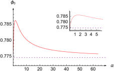
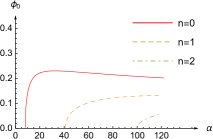
Figure 1: (Left) Plot of scalar hair $\phi_{0}(\alpha)=\bar{\phi}(r_{+},\alpha)\geq\bar{\phi}_{c}$ on the horizon as function of the coupling parameter $\alpha\in[0,\infty)$, showing a single branch. The dashed line denotes the constant scalar hairy black hole with $\phi_{0}=\bar{\phi}_{c}=0.7746=\phi_{\infty}$. (Right) Plots of $\phi_{0}(\alpha)=\bar{\phi}(r_{+},\alpha)$ for the first three branches among infinite branches. The $n=0$ branch starts from the first bifurcation point at $\alpha=8.019$, and $n=1$ and 2 branches start from the second point at $\alpha=40.84$ and from the third point at $\alpha=99.89$.

Explicitly, we wish to show a (numerical) scalarized charged black hole with $\alpha=63.75$ in Fig. 2. $N(r)$ and $\tilde{f}(r)$ represent metric function for scalarized charged black hole and constant scalar hairy black hole, respectively. The magnification in the left picture indicates an enlarged decrease of scalar hair $\phi(r)\geq\bar{\phi}_{c}$, showing a clear difference from a constant hair $\bar{\phi}_{c}=0.7746$ for the constant scalar hairy black hole [14]. It is worth noting that this scalar hair is not constant and does not blow up on the horizon and thus, it is surely a primary one.

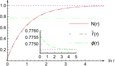
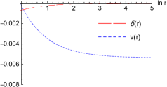
Figure 2: (Left) Plot of a scalarized black hole with $\alpha=63.75$, compared to the constant scalar hairy black hole [$\tilde{f}(r),~{}\bar{\phi}_{c}=0.7746$]. The horizon is located at $\ln r=\ln r_{+}=-0.0542$. The right picture indicates that $\delta(r)$ is negative [$\delta(r)=0$ for the constant scalar hairy black hole] and $v(r)$ is a negative function.

3.2 $n=0,1,2,\cdots$ scalarized charged black holes

In this case, an approach to finding infinite black hole solutions through the spontaneous scalarization is the nearly same in the previous one except that the the asymptotic solution in the far-region is given by

$$m(r) = M-\frac{3Q^{2}+Q_{s}^{2}}{6r}+\ldots,\quad\phi(r)=\frac{Q_{s}}{r}+\cdots,$$

$$\delta(r) = \frac{Q_{s}^{2}[2Q_{s}^{2}-6M^{2}+3Q^{2}(2+\alpha)]}{108r^{4}}+\cdots,\quad v(r)=\Psi+\frac{Q}{r}+\cdots,$$ (26)

whose limit of $\phi=0(Q_{s}=0)$ corresponds to the RN black hole. Actually, (3.2) could be obtained when imposing $\phi_{\infty}=0$ in (24). Thus, any asymptotic scalar hairs are absent in the far-region, differing from $\phi_{\infty}=\bar{\phi}_{c}$ found in the single branch of scalarized charged black holes. Here, we find that the blow-up points for $m(r)$ and $\delta(r)$ in (24) disappear. From (Right) Fig. 1, we have obtained the three branches of solutions labeled by $n=0(\alpha\geq 8.019),~{}n=1(\alpha\geq 40.84),~{}n=2(\alpha\geq 99.89)$ scalarized charged black holes. At this stage, we wish to note that the appearance of these black holes with scalar hair is closely connected to the onset of scalarization based on the instability of RN black holes determined by the linearized scalar equation (9) with $q=0.7$. Explicitly, we choose the horizon radius $r_{+}=0.857$ and electric charge $Q=0.35$ to construct the $n=0$ scalarized charged black hole with $\alpha=65.25$ shown in Fig. 3. Here $\phi(r)$ starts with $\phi_{0}(r_{+}=0.857,\alpha=65.25)=0.2196$ and its asymptotic value is zero.

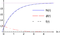
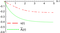
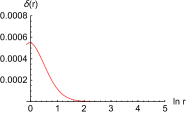
Figure 3: Graphs of a scalarized charged black hole with $\alpha=65.25$ in the $n=0$ branch. Here $f(r)$ and $\bar{A}_{t}$ represent the metric function and vector potential for the RN black hole with $\delta(r)=0$. We plot all figures in terms of ‘$\ln r$’ and thus, the horizon is located at $\ln r=\ln r_{+}=-0.154$.

4 Stability of scalarized charged black holes

Before we proceed, we have to mention that it is not an easy task to carry out the stability of scalarized charged black holes because these black holes come out as not analytic solutions but numerical solutions. In order to develop the stability analysis, one needs to obtain hundreds of numerical solutions depending on the coupling constant $\alpha$ in the each branch. Also, the full (axial+polar) perturbations require a complicated decoupling process because the linearized EMCS theory contains five physically propagating modes on these black hole background. In addition, we note that the $l=0$ ($s$-mode) scalar propagation determines mainly the stability of these black holes. In the conformal coupling theory (EMCS theory), it is would be better to choose the radial (spherically symmetric) perturbations starting with two metric and one vector perturbations which are regarded as a simpler version of the polar perturbation as far as the scalar perturbation is concerned.

Let us introduce the radial perturbations around the scalarized black holes as

$$ds^{2}_{\rm rad-p}=-N(r)e^{-2\delta(r)}(1+\epsilon H_{0})dt^{2}+\frac{dr^{2}}{N(r)(1+\epsilon H_{1})}+r^{2}\left(d\theta^{2}+\sin^{2}\theta d\varphi^{2}\right),$$

$$\phi(t,r)=\phi(r)+\epsilon\frac{\Phi(t,r)}{r},\quad F_{rt}(t,r)=v^{\prime}(r)+\epsilon\delta v(t,r),$$ (27)

where $N(r)$, $\delta(r)$, $\phi(r)$, and $v(r)$ represent a scalarized charged black hole background, while $H_{0}(t,r)$, $H_{1}(t,r)$, $\Phi(t,r)$, and $\delta v(t,r)$ denote four perturbed fields around the scalarized black hole background. From now on, we confine ourselves to analyzing the $l=0$($s$-mode) propagation, implying that higher angular momentum modes ($l\not=0$) are excluded. In this case, all perturbed fields except the perturbed scalar $\Phi$ may belong to redundant fields.

According to Appendix, we find the decoupled scalar equation for testing the stability of scalarized charged black holes as

$$\Big{[}g^{2}(r)\frac{\partial^{2}\Phi}{\partial t^{2}}\Big{]}-\frac{\partial^{2}\Phi}{\partial r^{2}}+C_{1}(r)\frac{\partial\Phi}{\partial r}+U(r)\Phi=0,\quad g(r)=\frac{e^{\delta(r)}}{N(r)},$$ (28)

where $C_{1}(r)$ and $U(r)$ are expressed in Appendix.

Introducing a further separation of $\Phi(t,r)=\delta\phi(r)e^{-i\omega t}$, we obtain the Schrödinger-like equation from (28)

$$\frac{d^{2}Z(r)}{dr_{*}^{2}}+[\omega^{2}-V(r,\alpha)]Z(r)=0,$$ (29)

where $r_{*}$ is a tortoise coordinate to extend from $r\in[r_{+},\infty]$ to $r_{*}\in[-\infty,\infty]$ and $Z(r)$ is a redefined scalar, expressed by

$$r_{*}=\int^{\infty}_{r_{+}}g(r)dr,~{}~{}Z(r)=\frac{\delta\phi(r)}{C_{0}(r)}.$$ (30)

Here the potential takes the form

$$V(r,\alpha)=\frac{U(r)-C^{\prime}_{1}(r)}{g^{2}(r)}+\frac{C_{1}g^{\prime}(r)+g^{\prime\prime}(r)}{g^{3}(r)}-\frac{[2g^{\prime}(r)]^{2}}{g^{4}(r)}.$$ (31)

We point out that $C_{0}(r)$ is the solution to the differential equation

$$[\ln C_{0}(r)]^{\prime}=C_{1}(r)-[\ln g(r)]^{\prime}$$ (32)

which means that it is difficult to solve for $C_{0}(r)$ analytically because of a complicated form $C_{1}(r)$.

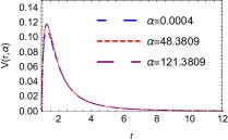
Figure 4: Scalar potential $V(r,\alpha)$ around scalarized charged black holes in the single branch. All potentials are positive definite outside the horizon for $\alpha>0$, implying the stable black hole.

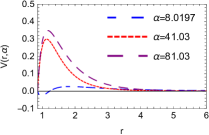
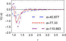
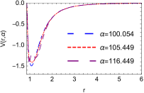
Figure 5: Scalar potentials $V(r,\alpha)$ around $n=0$ (Left: $\alpha\geq 8.019$), 1 (Middle: $\alpha\geq 40.84$), 2 (Right: $\alpha\geq 99.89$) black holes in the infinite branches.

Usually, a positive definite potential $V(r,\alpha)$ excluding any negative region guarantees the stability of the black hole. It is clear from Fig. 4 that the potential $V(r,\alpha)$ around the black hole in the single branch are positive definite outside the horizon for $\alpha>0$, indicating the stability. In this case, we do not need to perform a further analysis for stability. We inform from (Left) Fig. 5 that the potential around the $n=0$ black hole indicates large positive region outside the horizon, suggesting the stability. On the other hand, from (Middle, Right) Fig. 5, the potentials around the $n=1,2$ black holes show large negative regions outside the horizon, showing the instability. In addition, a sufficient condition for instability is given by $\int^{\infty}_{r_{+}}dr[g(r)V]<0$ in accordance with the existence of unstable modes [16]. However, a potential with negative region near the horizon whose integral ($\int^{\infty}_{r_{+}}dr[g(r)V]>0$) is positive might not exclude the existence of stable modes.

Importantly, to determine the (in)stability of the black hole, we have to solve (29) numerically by imposing an appropriate boundary condition that $Z(r)$ has an outgoing wave at infinity and an ingoing wave on the horizon: $Z(r)\sim e^{i\omega r_{*}}$ at $r_{*}\to\infty$ and $Z(r)\sim e^{-i\omega r_{*}}$ at $r_{*}\to-\infty$. If one finds an exponentially growing mode of $e^{\Omega t}(\omega=i\Omega)$, the corresponding black hole is unstable against the perturbation. The linearized scalar equation (29) around the scalarized charged black hole in the $n=0,1,2$ scalarized charged black holes may allow either a stable (decaying) mode with $\Omega<0$ or an unstable (growing) mode with $\Omega>0$. In case of unstable modes, we may solve (29) numerically with a boundary condition that $Z(r)=0$ at $r_{*}=\infty$ and $Z(r)=0$ at $r_{*}=-\infty$. We find from Fig. 6 that the $n=0$ black hole is stable against the $l=0$-scalar mode, whereas the $n=1,2$ black holes are unstable against the $l=0$-scalar mode.

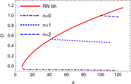
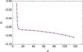
Figure 6: (Left) Plots of $\Omega$ as functions of $\alpha$ for $l=0$-scalar mode around the $n=0(\alpha\geq 8.019)~{},1(\alpha\geq 40.84),~{}2(\alpha\geq 99.89)$ black holes. The positive $\Omega$ for $n=1,2$ imply unstable black holes, while the negative $\Omega$ for $n=0$ shows a stable black hole. A red curve with $q=0.7$ denotes the positive $\Omega$ around the unstable RN black hole for $\alpha>8.019$. (Right) The enlarged picture shows the negative $\Omega$ for $\alpha\geq 8.019$ in the $n=0$ black hole clearly.

5 Stability of scalarized charged black holes with exponential coupling

The tachyonic instability of black holes without scalar hair triggering the spontaneous scalarization would be quenched by introducing a nonlinear scalar coupling term. In case of the EGBS theory, the scalarized black hole solutions in the pure quadratic coupling are always unstable [7, 17], whereas the scalarized black hole solutions in the nonlinear coupling models could be stable [17, 18, 19] because the nonlinear scalar terms may become more important as time passes and quench a growth of the scalar field. Furthermore, it was shown that the stability analysis of scalarized charged black holes makes no difference between quadratic coupling for the EMS theory [20] and exponential coupling [21]. This means that the $n=0$ black hole is stable, while the $n=1,2$ excited black holes are unstable, irrespective of coupling.

In this section, we wish to analyze the stability of scalarized charged black holes obtained from the EMCS theory with exponential coupling $\tilde{f}(\phi)=e^{\alpha\phi^{2}}$ whose limit of small amplitude reduces to the action (1) of the EMCS theory. We expect to derive a stable scalarized charged black hole. Here, we briefly describe scalarized charged black holes and their stability analysis without mentioning mathematical expressions because their mathematical expressions are similar to those in the EMCS theory (with quadratic coupling).

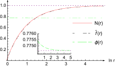
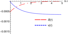
Figure 7: (Left) Plot of a scalarized black hole with $\alpha=9.6069$ in the single branch for exponential coupling. The horizon is located at $\ln r=\ln r_{+}=-0.0542$. $\tilde{f}(r)$ and $\bar{\phi}_{c}=0.7746$ represent the constant scalar hairy black hole. The right picture indicates $\delta(r)$ being a negative function and $v$ being a negative function .

First of all, we obtain a scalarized charged black hole solution in the single branch (see Fig. 7) and a scalarized charged black solution in the $n=0$ branch (see Fig. 8) by following Sec. 3 after replacing $1+\alpha\phi^{2}$ by exponential coupling $e^{\alpha\phi^{2}}$. In order to carry out their stability analyses, we redo the analysis in Sec. 4 after replacing after replacing $1+\alpha\phi^{2}$ by $e^{\alpha\phi^{2}}$.

Now, we obtain potential $V(r,\alpha)$ [Fig. 9] in the single branch and $V(r,\alpha)$ [Fig. 10] in the $n=0,~{}1,~{}2$ branches, which are very similar to the previous potentials in Figs. 4 and 5. The single branch and $n=0$ branch correspond to potentials with positive region, implying the stability. The other cases of $n=1$ and $2$ suggest instability of scalarized charged black holes because negative regions are larger than positive regions, leading to the sufficient condition for instability given by $\int^{\infty}_{r_{+}}dr[g(r)V]<0$.

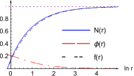
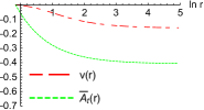
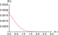
Figure 8: Graphs of a scalarized charged black hole with $\alpha=58.4167$ in the $n=0$ branch for exponential coupling. Here $f(r)$ and $\bar{A}_{t}$ represent the metric function and vector potential for the RN black hole with $\delta_{\rm RN}(r)=0$. The horizon is located at $\ln r=\ln r_{+}=-0.154$.

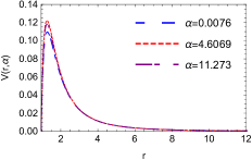
Figure 9: Scalar potential $V(r,\alpha)$ around scalarized charged black holes in the single branch for exponential coupling.

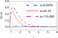
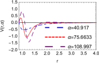
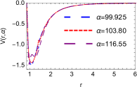
Figure 10: Scalar potentials $V(r,\alpha)$ around $n=0$ (Left: $\alpha\geq 8.019$), 1 (Middle: $\alpha\geq 40.84$), 2 (Right: $\alpha\geq 99.89$) black holes in the infinite branches for exponential coupling.

Actually, to determine the (in)stability of scalarized charged black holes, we have to solve the exponential version of (29) numerically by imposing an appropriate boundary condition that a redefined scalar $\tilde{Z}(r)$ has an outgoing wave at infinity and an ingoing wave on the horizon.

Finally, we find from Fig. 11 that the $n=0$ black hole is stable against the $l=0$-scalar because its $\Omega$ is negative, while the $n=1,2$ black holes are unstable against the $l=0$-scalar because their $\Omega$ are positive. This indicates that there is no change on stability of scalarized charged black holes when introducing the exponential coupling to the EMCS theory.

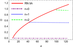
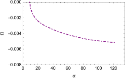
Figure 11: (Left) The positive $\Omega$ as functions of $\alpha$ for $l=0$-scalar around the $n=1(\alpha\geq 40.84),~{}2(\alpha\geq 99.89)$ black holes found in the EMCS theory with exponential coupling. A red curve with $q=0.7$ denotes the positive $\Omega$ of $l=0$-scalar as function of $\alpha$ around the RN black hole, indicating the unstable RN black holes for $\alpha>8.019$. (Right) The enlarged picture indicates the small negative $\Omega$ for $l=0$-scalar around the $n=0(\alpha\geq 8.019)$ black hole.

6 Discussions

First of all, we would like to mention that the black hole in the single branch and $n=0$ scalarized charged black hole found from the EMCS theory with both quadratic and exponential couplings are stable against the radial perturbations. The $n=1,2$ black holes obtained from the EMCS theory with both quadratic and exponential couplings are unstable against the radial perturbations. Actually, we note that there is no difference between radial and full perturbations as far as the $s$-mode scalar perturbation is concerned. It is worth noting that the stability results of $n=0,1,2$ black holes are consistent with those for the EMS theory [20, 21].

We summarize the stability issues for scalarized black holes obtained from three theories in Table 1. It implies that the inclusion of a conformally coupled scalar does not make any changes on the stability of scalarized charged black holes except that the EMCS theory admits a stable single branch additionally.

On the other hand, the stability analysis of scalarized (charged) black holes can replay for whether they could be the endpoints of tachyonic instability of black holes without scalar hair. Since the $n=0$ scalarized charged black hole obtained from the EMCS theory are stable, this is considered as an endpoint of the RN black hole.

However, it is unclear that the scalarized charged black hole in the single branch will radiate to yield the constant scalar hairy black hole because two are stable.

Theory	$n=0$	$n=1$	$n=2$	Single Branch	Perturbations	Reference
EGBS with EC	NA	NA	NA	U(SBH)	Radial	[6, 7, 22]
EGBS with EC	S	U	U	NA	Radial	[17]
EGBS with QC	U	U	U	NA	Radial	[17]
EGBS with qC	S	U	U	NA	Radial	[18],[19]
EGBS with EC	S	$\cdot$	$\cdot$	NA	Axial	[23]
EMS with EC	NA	NA	NA	U(RNBH)	Radial	[10]
EMS with EC	S	U	U	NA	Full	[21]
EMS with QC	S	U	U	NA	Full	[20]
EMCS with QC	S	U	U	S	Radial	This work
EMCS with EC	S	U	U	S	Radial	This work

Table 1: Summary of stability analysis for scalarized black holes obtained from three theories. EGBS stands for Einstein-Gauss-Bonnet-Scalar and EMS denotes Einstein-Maxwell-Scalar. EC, QC, and qC represent exponential coupling, quadratic coupling, quartic coupling. U(S) indicates unstable (stable) black hole. Full implies axial+polar. SBH (RNBH) mean Schwarzschild (Reissner-Norström) black holes without scalar hair, known as the GR solutions. Finally, NA represents not available and ‘$\cdot$’ implies not computed.

Acknowledgments

This work was supported by the National Research Foundation of Korea (NRF) grant funded by the Korea government (MOE) (No. NRF-2017R1A2B4002057).

Appendix

In Appendix, we wish to derive a decoupled linearized scalar equation (28)[=(47)]. Expanding equation (2) up to the first order $\epsilon(\epsilon\ll 1)$, we obtain the seven-coupled linearized equations. Four equations of $(t,t)$, $(t,r)$, $(r,r)$, and $(\theta,\theta)$-component are given by

$$(t,r):\quad A_{0}H_{1}+A_{1}\Phi+A_{2}\Phi^{\prime}=0,$$ (33)

$$(t,t):\quad-\frac{A_{2}}{g^{2}}\Phi^{\prime\prime}+A_{3}\Phi^{\prime}+A_{4}\Phi+A_{5}H_{1}-\frac{A_{0}}{g^{2}}H_{1}^{\prime}+A_{6}H_{0}+A_{7}\delta v=0,$$ (34)

$$(r,r):\quad-A_{7}g^{2}\delta v-A_{2}g^{2}\ddot{\Phi}+A_{8}\Phi^{\prime}+A_{9}\Phi+A_{10}H_{1}+A_{0}H_{0}^{\prime}+A_{11}H_{0}=0,$$ (35)

$$(\theta,\theta):\quad B_{0}\delta v+B_{1}H_{0}+B_{2}\Phi+B_{3}H_{0}^{\prime}+B_{4}H_{1}^{\prime}+B_{5}\Phi^{\prime}+B_{6}\Phi^{\prime\prime}$$

$$\qquad\qquad+B_{7}H_{0}^{\prime\prime}+B_{8}\ddot{H}_{1}+B_{9}\ddot{\Phi}=0$$ (36)

with $g^{2}(r)=\frac{e^{2\delta(r)}}{N^{2}(r)}$. Here, the overdot ($\dot{{}}$) denotes derivative with respect to time $t$, and $A_{i}(i=0,1,\cdots,11)$ and $B_{i}(i=0,1,\cdots,10)$ are functions of $r$ given by

$$A_{0}=-\frac{\phi^{2}-3+r\phi\phi^{\prime}}{3},\quad A_{1}=\frac{1}{3}(\frac{2\phi}{r}+\frac{\phi N^{\prime}}{N}-2\phi\delta^{\prime}+4\phi^{\prime}),$$

$$A_{2}=-\frac{2\phi}{3},\quad A_{3}=\frac{e^{-2\delta}N(\phi N^{\prime}-2N\phi^{\prime})}{3r},$$

$$A_{4}=\frac{e^{-2\delta}N}{3r^{3}}\left(\phi(2N-2+rN^{\prime}-6e^{2\delta}\alpha r^{2}v^{\prime 2})+r(rN^{\prime}\phi^{\prime}+2N(3\phi^{\prime}+r\phi^{\prime\prime}))\right),$$

$$A_{5}=\frac{e^{-2\delta}N}{3r^{2}}\left(r(-3e^{2\delta}r(1+\alpha\phi^{2})v^{\prime 2}+N^{\prime}(\phi^{2}-3+r\phi\phi^{\prime}))\right.$$

$$\qquad\left.+N(-3+\phi^{2}-r^{2}\phi^{\prime 2}+2r\phi(2\phi^{\prime}+r\phi^{\prime\prime}))\right),$$

$$A_{6}=\frac{e^{-2\delta}N}{3r^{2}}\left(3-3rN^{\prime}+\phi^{2}(rN^{\prime}-1)+r^{2}\phi N^{\prime}\phi^{\prime}+N(\phi^{2}-3-r^{2}\phi^{\prime 2}+2r\phi(2\phi^{\prime}+r\phi^{\prime\prime})\right),$$

$$A_{7}=-2N(1+\alpha\phi^{2})v^{\prime},$$

$$A_{8}=\frac{1}{3r^{2}N}\left(-r\phi N^{\prime}+2N(\phi(-2+r\delta^{\prime})-3r\phi^{\prime}\right),$$

$$A_{9}=\frac{1}{3r^{2}N}\left(\phi(2-2rN^{\prime}+6\alpha e^{2\delta}r^{2}v^{\prime 2}+N(4r\delta^{\prime}-2))+r(-rN^{\prime}+2N(r\delta^{\prime}-2))\phi^{\prime}\right),$$

$$A_{10}=-\frac{\phi^{2}-3}{3r^{2}N},\quad A_{11}=-\frac{e^{2\delta}(1+\alpha\phi^{2})v^{\prime 2}}{N},$$

$$B_{0}=-2e^{2\delta}r^{2}(1+\alpha\phi^{2})v^{\prime},\quad B_{1}=e^{2\delta}r^{2}(1+\alpha\phi^{2})v^{\prime 2},$$

$$B_{2}=\frac{2\phi\left(e^{2\delta}r(9+18\alpha+\alpha\phi^{4})v^{\prime 2}-3N\phi^{\prime}(2\phi+r\phi^{\prime})\right)}{9(\phi^{2}-3)}-\frac{2\phi}{3r}(N-rN^{\prime}+rN\delta^{\prime}),$$

$$B_{3}=\frac{r}{12}\left(-3r(-3+\phi^{2})N^{\prime}+2N(3-6r\delta^{\prime}+\phi^{2}(2r\delta^{\prime}-1)-2r\phi\phi^{\prime})\right),$$

$$B_{4}=\frac{r}{12}\left(-r(-3+\phi^{2})N^{\prime}+2N(3-3r\delta^{\prime}+\phi^{2}(r\delta^{\prime}-1)-2r\phi\phi^{\prime})\right),$$

$$B_{5}=\frac{2r}{3}\left(-r\phi N^{\prime}+N(\phi(r\delta^{\prime}+1)+r\phi^{\prime})\right),\quad B_{6}=-\frac{2rN\phi}{3},$$

$$B_{7}=-\frac{r^{2}(\phi^{2}-3)N}{6},\quad B_{8}=-\frac{r^{2}(\phi^{2}-3)e^{2\delta}}{6N},\quad B_{9}=\frac{2e^{2\delta}r\phi}{3N}.$$ (37)

Two linearized Maxwell equations take the forms

$$\nu=t:\quad A_{12}\delta v+A_{13}\delta v^{\prime}+A_{14}\Phi^{\prime}+A_{15}\Phi+A_{16}(H_{0}^{\prime}-H_{1}^{\prime})=0,$$ (38)

$$\nu=r:\quad A_{13}\delta\dot{v}+A_{14}\dot{\Phi}+A_{16}(\dot{H_{0}}-\dot{H_{1}})=0,$$ (39)

where

$$A_{12}=e^{2\delta}\left((1+\alpha\phi^{2})(\frac{2}{r}+\delta^{\prime})+2\alpha\phi\phi^{\prime}\right),\quad A_{13}=e^{2\delta}(1+\alpha\phi^{2}),\quad A_{14}=\frac{2\alpha e^{2\delta}\phi v^{\prime}}{r},$$

$$A_{15}=-\frac{2\alpha e^{2\delta}v^{\prime}}{r^{2}}-\frac{2\alpha e^{2\delta}(-1+\alpha\phi^{2})\phi^{\prime}v^{\prime}}{r(1+\alpha\phi^{2})},\quad A_{16}=-\frac{1}{2}e^{2\delta}(1+\alpha\phi^{2})v^{\prime}.$$ (40)

Finally, one has a linearized scalar equation

$$B_{10}\delta v+B_{11}H_{0}+B_{12}\Phi+B_{13}H_{1}+B_{14}H_{0}^{\prime}+B_{15}H_{1}^{\prime}+B_{16}\Phi^{\prime}+B_{17}\Phi^{\prime\prime}$$

$$+B_{18}H_{0}^{\prime\prime}+B_{19}\ddot{H}_{1}+B_{20}\ddot{\Phi}=0$$ (41)

with

$$B_{10}=2\alpha e^{2\delta}\phi v^{\prime},\quad B_{11}=-\alpha e^{2\delta}\phi v^{\prime 2},$$

$$B_{12}=-\frac{3N^{\prime}+e^{2\delta}r\alpha(\phi^{2}-3)v^{\prime 2}-3N\delta^{\prime}}{3r^{2}},\quad B_{13}=\frac{\phi}{3r^{2}},$$

$$B_{14}=\frac{N\phi^{\prime}}{3r}+\frac{\phi}{12}\left(3N^{\prime}-4N\delta^{\prime}\right)+\frac{N\phi^{\prime}}{2},$$

$$B_{15}=\frac{N\phi^{\prime}}{3r}+\frac{\phi}{12}\left(N^{\prime}-2N\delta^{\prime}\right)+\frac{N\phi^{\prime}}{2},$$

$$B_{16}=\frac{N^{\prime}-N\delta^{\prime}}{r},\quad B_{17}=\frac{N}{r},\quad B_{18}=\frac{N\phi}{6},$$

$$B_{19}=\frac{e^{2\delta}\phi}{6N},\quad B_{20}=\frac{2e^{2\delta}r\phi}{3N}.$$ (42)

Now, our main task is to diagonalize the linerized scalar equation (41) by exploiting the remaining six equations. From (33), we have

$$H_{1}=-\frac{A_{1}}{A_{0}}\Phi-\frac{A_{2}}{A_{0}}\Phi^{\prime}$$ (43)

which implies that $H_{1}$ is a redundant field. Integrating (39) with respect to $t$ leads to $\delta v$

$$\delta v=-\frac{A_{14}}{A_{13}}\Phi-\frac{A_{16}}{A_{13}}(H_{0}-H_{1})$$ (44)

which means that $\delta v$ is also a redundant field. Using (36), we transform (41) to a reduced scalar equation without $H_{0}^{\prime\prime}$ and $\ddot{H}_{1}$

$$A_{17}(H_{0}^{\prime}+H_{1}^{\prime})+A_{18}\Phi^{\prime\prime}-A_{18}g^{2}\ddot{\Phi}+A_{19}\delta v+A_{20}\Phi^{\prime}+A_{21}\Phi+A_{22}H_{0}+A_{23}H_{1}=0,$$ (45)

where

$$A_{17}=\frac{rN^{2}}{36}\left((\phi^{2}-3)\phi+(\phi^{2}-9)r\phi^{\prime}\right),\quad A_{18}=\frac{r^{2}N^{2}}{18}(\phi^{2}-9),\quad A_{19}=-e^{2\delta}r^{2}(\frac{1}{3}+\alpha)N\phi v^{\prime},$$

$$A_{20}=\frac{N}{18}\left(r(\phi^{2}-9)N^{\prime}+N(\phi^{2}(2-r\delta^{\prime})+9r\delta^{\prime}+2r\phi\phi^{\prime})\right),$$

$$A_{21}=-\frac{N}{18r(\phi^{2}-3)}\left(-(\phi^{2}-3)^{2}-18rN^{\prime}+3e^{2\delta}r^{2}(1+3\alpha)(3+\phi^{2})v^{\prime 2}+6r\phi N^{\prime}(\phi+2r\phi^{\prime})\right)$$

$$\qquad+\frac{N^{2}}{18r(\phi^{2}-3)}\left(\phi^{4}-2r\phi^{3}\phi^{\prime}-6r\phi(2r\phi^{\prime}-3)\phi^{\prime}+r\phi^{2}(r\phi^{\prime 2}+6\delta^{\prime})-3(r^{2}\phi^{\prime 2}-6r\delta^{\prime}-3)\right)$$

$$\qquad+\frac{2N^{2}r\phi\phi^{\prime\prime}}{3(\phi^{2}-3)},$$

$$A_{22}=e^{2\delta}r^{2}(\frac{1}{6}+\frac{\alpha}{2})N\phi v^{\prime 2},$$

$$A_{23}=\frac{rNN^{\prime}}{18}\left((\phi^{2}-3)\phi+(\phi^{2}-9)r\phi^{\prime}\right)-e^{2\delta}r^{2}(\frac{1}{6}+\frac{\alpha}{2})N\phi v^{\prime 2}+\frac{r^{2}N^{2}}{18}(\phi^{2}-9)\phi^{\prime\prime}$$

$$\qquad+\frac{N^{2}}{18}\left(\phi^{3}(1-r\delta^{\prime})+r\phi^{2}\phi^{\prime}(4-r\delta^{\prime})+9r\phi^{\prime}(r\delta^{\prime}-2)+\phi(3r\delta^{\prime}+r^{2}\phi^{\prime 2}-3)\right).$$ (46)

Making use of (44), (43), $\delta v^{\prime}$, and $H_{1}^{\prime}$, we could express (45) in terms of $H_{0}^{\prime}$, $\Phi$, $\Phi^{\prime}$ and $\Phi^{\prime\prime}$: called the reduced (45). Combining (35) with the reduced (45) to eliminate $H_{0}^{\prime}$ arrives at the master scalar equation for testing the stability of scalarized charged black holes as

$$\Big{[}g^{2}(r)\frac{\partial^{2}\Phi}{\partial t^{2}}\Big{]}-\frac{\partial^{2}\Phi}{\partial r^{2}}+C_{1}(r)\frac{\partial\Phi}{\partial r}+U(r)\Phi=0,$$ (47)

where $C_{1}(r)$ is expressed as

$$C_{1} = \frac{C_{2}}{C_{3}}+\frac{C_{4}}{3NC_{3}},$$

$$C_{2} = r\phi(\phi^{2}-3)^{2}(63-\phi^{2}+r(2\phi^{2}-45)\delta^{\prime})\phi^{\prime}+r^{2}(\phi^{2}-3)\left(\phi^{2}(150-\phi^{2}+r(\phi^{2}-36)\delta^{\prime})-135\right)\phi^{\prime 2}$$

$$+r^{3}\phi(\phi^{4}+84\phi^{2}-351)\phi^{\prime 3}+r^{4}\phi^{2}(\phi^{2}-9)\phi^{\prime 4}+(\phi^{2}-3)^{3}(9+r(\phi^{2}-9)\delta^{\prime}),$$

$$C_{3} = 9r(\phi^{2}-3)(\phi^{2}-3+r\phi\phi^{\prime}),$$

$$C_{4} = 729(e^{2\delta}r^{2}v^{\prime 2}-1)(r\phi^{\prime}\phi-1)+81\phi^{2}\left(r^{2}(-\phi^{\prime 2}+e^{2\delta}v^{\prime 2}(6-15\alpha+r^{2}\phi^{\prime 2}))-9\right)$$ (48)

$$+27\phi^{3}\phi^{\prime}r\left(17+2e^{2\delta}r^{2}v^{\prime 2}(15\alpha-4)\right)+9\phi^{4}\left(27+r^{2}(4\phi^{\prime 2}+e^{2\delta}v^{\prime 2}(105\alpha-9+r^{2}(12\alpha-1)\phi^{\prime 2}))\right)$$

$$-9\phi^{5}\phi^{\prime}r\left(7+e^{2\delta}v^{\prime 2}r^{2}(28\alpha+1))-3\phi^{6}(9+r^{2}(\phi^{\prime 2}+\alpha e^{2\delta}v^{\prime 2}(72+7r^{2}\phi^{\prime 2}))\right)$$

$$-3\phi^{7}\phi^{\prime}r(1+4\alpha e^{2\delta}v^{\prime 2}r^{2})+\alpha\phi^{8}e^{2\delta}v^{\prime 2}r^{2}(9+r^{2}\phi^{\prime 2})+2\alpha\phi^{9}e^{2\delta}v^{\prime 2}r^{3}\phi^{\prime}+\alpha\phi^{10}e^{2\delta}v^{\prime 2}r^{2}.$$

On the other hand, $U(r)$ takes a complicated form as

$$U = \frac{U_{2}}{U_{1}},$$

$$U_{1} = 54r^{2}N^{2}\phi(\phi^{2}-3)^{2}(1+\alpha\phi^{2})(-3+\phi^{2}+r\phi\phi^{\prime}),$$

$$U_{2} = D_{0}+\phi D_{1}+\phi^{2}D_{2}+\phi^{3}D_{3}+\phi^{4}D_{4}+\phi^{5}D_{5}+\phi^{6}D_{6}+\phi^{7}D_{7}+\phi^{8}D_{8}+\phi^{9}D_{9}+\phi^{10}D_{10}$$ (49)

$$+\phi^{11}D_{11}+\phi^{12}D_{12}+\phi^{13}D_{13}$$

with

$$D_{0} = 1458r^{2}N^{2}\phi^{\prime}(3\delta^{\prime}+2r\phi^{\prime 2}),$$

$$D_{1} = -162N\left(3(1-e^{2\delta}r^{2}(1+3\alpha)v^{\prime 2}+rN^{\prime}(2-7r^{2}\phi^{\prime 2}))\right.$$

$$\left.+N(-3+r(-15\delta^{\prime}+r(33r\delta^{\prime}-35)\phi^{\prime 2}+6r^{3}\phi^{\prime 4}))\right),$$

$$D_{2} = 81r\phi^{\prime}\left(6r^{2}N^{\prime 2}+2N^{2}(8-18\alpha+r(\delta^{\prime}(27\alpha-53+3r\delta^{\prime})+2r(6(\alpha-2)+r\delta^{\prime})\phi^{\prime 2}))\right.$$

$$\left.+N(-8+36\alpha+r(4e^{2\delta}r(6\alpha-1)v^{\prime 2}-N^{\prime}(-38+36\alpha+15r\delta^{\prime}+2r^{2}\phi^{\prime 2})))\right),$$

$$D_{3} = -9\left(-9r^{3}N^{\prime}(6\alpha e^{2\delta}v^{\prime 2}+rN^{\prime}\phi^{\prime 2})+2N^{2}(9(2+3\alpha+r\delta^{\prime}(18-15\alpha+r\delta^{\prime}))\right.$$

$$\left.-9r^{2}(-28+39\alpha+r\delta^{\prime}(26-21\alpha+2r\delta^{\prime}))\phi^{\prime 2}+r^{4}(36\alpha-19)\phi^{\prime 4})\right.$$

$$\left.+3N(rN^{\prime}(-42+72\alpha-3r\delta^{\prime}+2r^{2}(50-63\alpha+6r\delta^{\prime})\phi^{\prime 2})+2(-6-9\alpha+r^{2}(18\alpha-5)\phi^{\prime 2}\right.$$

$$\left.+e^{2\delta}v^{\prime 2}(3+3\alpha(8+27\alpha)+r(18\alpha\delta^{\prime}-r(1+3\alpha)\phi^{\prime 2})))))\right),$$

$$D_{4} = 27r^{3}N^{\prime}\phi^{\prime}\left((18\alpha-11)N^{\prime}+3e^{2\delta}r\alpha v^{\prime 2}\right)$$

$$+2N^{2}\left(72-270\alpha+3r\delta^{\prime}(-86+147\alpha+3r(1-3\alpha)\delta^{\prime})+2r^{2}(-31+84\alpha+3(r+3r\alpha)\delta^{\prime})\phi^{\prime 2}\right)$$

$$+3N\left(4(39\alpha-5)+6e^{2\delta}r^{2}\alpha v^{\prime 2}(9-24\alpha+r\delta^{\prime})+rN^{\prime}(82-234\alpha\right)$$

$$\left.+r(5(9\alpha-5)\delta^{\prime}-2r(1+3\alpha)\phi^{\prime 2}))\right),$$

$$D_{5} = 9r^{3}N^{\prime}\left(3e^{2\delta}\alpha(18\alpha-17)v^{\prime 2}+r(9\alpha-4)N^{\prime}\phi^{\prime 2}\right)+18N^{2}\left(54\alpha+9r\delta^{\prime}(8-18\alpha+(r-r\alpha)\delta^{\prime})\right.$$

$$\left.+r^{2}(65-276\alpha+r\delta^{\prime}(-49+138\alpha+2r(9\alpha-4)\delta^{\prime}))\phi^{\prime 2}+r^{4}(11\alpha-1)\phi^{\prime 4}\right)$$

$$9N\left(-108\alpha+r(6r(19\alpha-2)\phi^{\prime 2}+2e^{2\delta}rv^{\prime 2}(-3+3\alpha(17+99\alpha)+3r(17-18\alpha)\alpha\delta^{\prime}\right.$$

$$\left.+r^{2}(\alpha-1)(9\alpha-1)\phi^{\prime 2})+N^{\prime}(54(5\alpha-1)+9r(\alpha-1)\delta^{\prime}+2r^{2}(31-144\alpha+2r(4-9\alpha)\delta^{\prime})\phi^{\prime 2}))\right),$$

$$D_{6} = 9r\phi^{\prime}\left(r^{2}N^{\prime}((4-33\alpha)N^{\prime}+e^{2\delta}r\alpha(9\alpha-7)v^{\prime 2})+2N^{2}(24-162\alpha+r(\delta^{\prime}(-49+222\alpha\right.$$

$$\left.-3(r+3r\alpha)\delta^{\prime})+2r(-2+24\alpha+5r\alpha\delta^{\prime})\phi^{\prime 2}))+N(-16+240\alpha-2e^{2\delta}r^{2}v^{\prime 2}(-2+\alpha(5+147\alpha)\right.$$

$$\left.+r\alpha(-7+9\alpha)\delta^{\prime})-5rN^{\prime}(-10+78\alpha+r((1-15\alpha)\delta^{\prime}+2r\alpha\phi^{\prime 2})))\right),$$

$$D_{7} = -3r^{2}N^{\prime}\left(9e^{2\delta}\alpha(17\alpha-5)v^{\prime 2}+r(12\alpha-1)N^{\prime}\phi^{\prime 2}\right)+6N^{2}\left(-6+108\alpha+3r\delta^{\prime}(14-72\alpha\right.$$

$$\left.+3r(1-3\alpha)\delta^{\prime})+r^{2}(16-207\alpha+r\delta^{\prime}(-4+63\alpha+2r(12\alpha-1)\delta^{\prime}))\phi^{\prime 2}+r^{4}\alpha\phi^{\prime 4}\right)$$

$$-3N\left(12-216\alpha+r(N^{\prime}(6(63\alpha-5)+9r(3\alpha-1)\delta^{\prime})+2r^{2}(2-81\alpha+2r(1-12\alpha)\delta^{\prime})\phi^{\prime 2})\right.$$

$$\left.+2r((48\alpha-1)\phi^{\prime 2}+e^{2\delta}v^{\prime 2}(-3+9\alpha(7+36\alpha)+r\alpha(9(5-17\alpha)\delta^{\prime}+r(51\alpha-19)\phi^{\prime 2})))\right),$$

$$D_{8} = -3r\phi^{\prime}\left(r^{2}N^{\prime}(-(1+12\alpha)N^{\prime}+e^{2\delta}r\alpha(21\alpha-5)v^{\prime 2})+2N^{2}(8-126\alpha\right.$$

$$\left.+r(\delta^{\prime}(-7+111\alpha+3r(3\alpha-1)\delta^{\prime})+4r\alpha(2+r\delta^{\prime})\phi^{\prime 2}))+N(-4+156\alpha\right.$$

$$\left.-2e^{2\delta}r^{2}\alpha v^{\prime 2}(19+21\alpha+r(21\alpha-5)\delta^{\prime})+rN^{\prime}(6-222\alpha+r(5(1+3\alpha)\delta^{\prime}-4r\alpha\phi^{\prime 2})))\right),$$

$$D_{9} = 3\alpha r^{3}N^{\prime}\left(3e^{2\delta}(15\alpha-1)v^{\prime 2}+rN^{\prime}\phi^{\prime 2}\right)+6N^{2}\left(30\alpha-1+r(\delta^{\prime}(3-42\alpha+(r-9\alpha r)\delta^{\prime})\right.$$

$$\left.+2\alpha r(r\delta^{\prime}-4)(2+r\delta^{\prime})\phi^{\prime 2})\right)+3N\left(2-60\alpha+r(-N^{\prime}(2-78\alpha+\delta^{\prime}(r-9r\alpha+4\alpha r^{3}\phi^{\prime 2}))\right.$$

$$\left.+2r\alpha(3\phi^{\prime 2}+e^{2\delta}v^{\prime 2}(8+18\alpha+3r((1-15\alpha)\delta^{\prime}+8r\alpha\phi^{\prime 2}))))\right),$$

$$D_{10} = -\alpha e^{2\delta}v^{\prime 2}r^{3}\left((1-15\alpha)rN^{\prime}+2N(-1-75\alpha+r(15\alpha-1)\delta^{\prime})\right)\phi^{\prime}$$

$$-3r\alpha\phi^{\prime}\left(-r^{2}N^{\prime 2}-6N^{2}(-4+r\delta^{\prime}(1+r\delta^{\prime}))+N(-12+5rN^{\prime}(2+r\delta^{\prime}))\right),$$

$$D_{11} = 3\alpha N\left(6-rN^{\prime}(6+r\delta^{\prime})+2N(-3+r\delta^{\prime}(3+r\delta^{\prime}))\right)$$

$$-e^{2\delta}\alpha r^{2}v^{\prime 2}\left(r(1+9\alpha)N^{\prime}-2N(1+27\alpha+r(1+9\alpha)\delta^{\prime})+8\alpha r^{2}N\phi^{\prime 2}\right),$$

$$D_{12} = e^{2\delta}v^{\prime 2}r^{3}\alpha^{2}\left(2N(r\delta^{\prime}-7)-rN^{\prime}\right),$$

$$D_{13} = e^{2\delta}v^{\prime 2}r^{2}\alpha^{2}\left(2N(r\delta^{\prime}-3)-rN^{\prime}\right).$$ (51)

Finally, we wish to mention that two equations (34) and (38) are redundant.

References

[1]
R. Ruffini and J. A. Wheeler,
Phys. Today 24, no. 1, 30 (1971).
doi:10.1063/1.3022513
[2]
C. A. R. Herdeiro and E. Radu,
Int. J. Mod. Phys. D 24, no. 09, 1542014 (2015)
doi:10.1142/S0218271815420146
[arXiv:1504.08209 [gr-qc]].
[3]
N. M. Bocharova, K. A. Bronnikov and V. N. Melnikov,
Vestn. Mosk. Univ. Ser. III Fiz. Astron. , no. 6, 706 (1970).
[4]
J. D. Bekenstein,
Annals Phys. 82, 535 (1974).
doi:10.1016/0003-4916(74)90124-9
[5]
M. Astorino,
Phys. Rev. D 88, no. 10, 104027 (2013)
doi:10.1103/PhysRevD.88.104027
[arXiv:1307.4021 [gr-qc]].
[6]
D. D. Doneva and S. S. Yazadjiev,
Phys. Rev. Lett. 120, no. 13, 131103 (2018)
doi:10.1103/PhysRevLett.120.131103
[arXiv:1711.01187 [gr-qc]].
[7]
H. O. Silva, J. Sakstein, L. Gualtieri, T. P. Sotiriou and E. Berti,
Phys. Rev. Lett. 120, no. 13, 131104 (2018)
doi:10.1103/PhysRevLett.120.131104
[arXiv:1711.02080 [gr-qc]].
[8]
G. Antoniou, A. Bakopoulos and P. Kanti,
Phys. Rev. Lett. 120, no. 13, 131102 (2018)
doi:10.1103/PhysRevLett.120.131102
[arXiv:1711.03390 [hep-th]].
[9]
C. A. R. Herdeiro, E. Radu, N. Sanchis-Gual and J. A. Font,
Phys. Rev. Lett. 121, no. 10, 101102 (2018)
doi:10.1103/PhysRevLett.121.101102
[arXiv:1806.05190 [gr-qc]].
[10]
Y. S. Myung and D. C. Zou,
Eur. Phys. J. C 79, no. 3, 273 (2019)
doi:10.1140/epjc/s10052-019-6792-6
[arXiv:1808.02609 [gr-qc]].
[11]
P. G. Fernandes, C. A. Herdeiro, A. M. Pombo, E. Radu and N. Sanchis-Gual,
Class. Quant. Grav. 36, no.13, 134002 (2019)
doi:10.1088/1361-6382/ab23a1
[arXiv:1902.05079 [gr-qc]].
[12]
D. Astefanesei, C. Herdeiro, A. Pombo and E. Radu,
JHEP 10, 078 (2019)
doi:10.1007/JHEP10(2019)078
[arXiv:1905.08304 [hep-th]].
[13]
J. L. Blázquez-Salcedo, C. A. Herdeiro, J. Kunz, A. M. Pombo and E. Radu,
Phys. Lett. B 806, 135493 (2020)
doi:10.1016/j.physletb.2020.135493
[arXiv:2002.00963 [gr-qc]].
[14]
D. C. Zou and Y. S. Myung,
Phys. Lett. B 803, 135332 (2020)
doi:10.1016/j.physletb.2020.135332
[arXiv:1911.08062 [gr-qc]].
[15]
M. Khodadi, A. Allahyari, S. Vagnozzi and D. F. Mota,
arXiv:2005.05992 [gr-qc].
[16]
G. Dotti and R. J. Gleiser,
Class. Quant. Grav. 22, L1 (2005)
doi:10.1088/0264-9381/22/1/L01
[gr-qc/0409005].
[17]
J. L. Blázquez-Salcedo, D. D. Doneva, J. Kunz and S. S. Yazadjiev,
Phys. Rev. D 98, no. 8, 084011 (2018)
doi:10.1103/PhysRevD.98.084011
[arXiv:1805.05755 [gr-qc]].
[18]
M. Minamitsuji and T. Ikeda,
Phys. Rev. D 99, no. 4, 044017 (2019)
doi:10.1103/PhysRevD.99.044017
[arXiv:1812.03551 [gr-qc]].
[19]
H. O. Silva, C. F. B. Macedo, T. P. Sotiriou, L. Gualtieri, J. Sakstein and E. Berti,
Phys. Rev. D 99, no. 6, 064011 (2019)
doi:10.1103/PhysRevD.99.064011
[arXiv:1812.05590 [gr-qc]].
[20]
Y. S. Myung and D. C. Zou,
Eur. Phys. J. C 79, no. 8, 641 (2019)
doi:10.1140/epjc/s10052-019-7176-7
[arXiv:1904.09864 [gr-qc]].
[21]
Y. S. Myung and D. C. Zou,
Phys. Lett. B 790, 400 (2019)
doi:10.1016/j.physletb.2019.01.046
[arXiv:1812.03604 [gr-qc]].
[22]
Y. S. Myung and D. C. Zou,
Phys. Rev. D 98, no. 2, 024030 (2018)
doi:10.1103/PhysRevD.98.024030
[arXiv:1805.05023 [gr-qc]].
[23]
J. L. Blázquez-Salcedo, D. D. Doneva, S. Kahlen, J. Kunz, P. Nedkova and S. S. Yazadjiev,
Phys. Rev. D 101, no. 10, 104006 (2020)
doi:10.1103/PhysRevD.101.104006
[arXiv:2003.02862 [gr-qc]].