Federated Recommendation System via Differential Privacy

Abstract

In this paper we are interested in what we term the federated private bandits framework, that combines differential privacy with multi-agent bandit learning. We explore how differential privacy based Upper Confidence Bound (UCB) methods can be applied to multi-agent environments, and in particular to federated learning environments both in ‘master-worker’ and ‘fully decentralized’ settings. We provide theoretical analysis on the privacy and regret performance of the proposed methods and explore the tradeoffs between these two.

I Introduction

The promise of distributed computing is to improve the efficiency and robustness of machine learning tasks by leveraging communication networks to share the computational load, leading to a compelling vision of world-wide computing [1]. However, no matter how compelling this vision is, it cannot get realized before we address a number of challenges, of which an important one is privacy.

In this paper, we consider privacy vs. learning trade-offs for wireless recommendation systems, that are one of the most popular learning algorithms in the consumer domain, and are considered a key application of edge-based wireless distributed systems [2] [3] [4]. As a use case, we consider a multi-chain of stores, such as a fastfood chain, that make local recommendations to their customers, but then wish to aggregate the overall client responses to provide new recommendations or launch new products. We assume that the client responses - what items they like and how much - are the private data we want to protect.

We pose our problem within the federated learning framework, proposed by Google[5], that addresses the privacy challenge by maintaining the user data locally, while combining learning models among the distributed agents. In particular, we consider a federated multi-armed bandit (MAB) setup, where each distributed agent could be a local store that makes recommendations, while the aggregator is the parent company. The question we explore is, can we leverage the aggregator to better inform what recommendations to make at the distributed agents, without compromising the user data privacy.

We consider in particular a distributed version of the UCB algorithm: we assume that each agent (store) makes a number of recommendations locally and calculates a sequence of local average reward values. To combine the local models, we need to reveal the average values sequence to the aggregator, without compromising the privacy of the data. We do so by leveraging differential privacy (DP) [6] techniques that preserve privacy of reward sequences. Maintaining privacy amounts to adding a form of noise, which can affect which items the aggregator decides to recommend next, and which in turn can lead to a higher regret. This paper investigates this privacy/regret trade-off.

I-A Related Work

The MAB algorithm is widely used in recommendation systems due to its simplicity and efficiency [7][8]. Auer et al. [9] developed the UCB algorithm, which is an index-based policy relying on average reward plus an upper confidence bound. Another mainstream approach is the sampling-based approach [10] that instead of computing a deterministic index, it uses a sample generated by a Bayesian estimator.

There has been a growing literature that extends the MAB problem into multi-user settings. Liu and Zhao [11] consider a distributed bandit problem with collisions: choosing the same arm simultaneously leads to a reduced reward for two or more agents. Similar approaches can be found in [12] [13] that utilize different matching algorithms to avoid collisions. Later work [14] makes use of gossip algorithm or running consensus methods to keep an approximation of the average value between agents and their neighbors. However, few works have considered accommodating privacy considerations in the learning process.

There is also a very rich literature on differential privacy, mostly applied in deep learning[15] and information theory fields. For decision-making problems, Tossou and Dimitrakakis present algorithms for differentially private stochastic MAB [16]. The work in [17] also investigates this problem. However, all these works operate under a single user setting. As far as we know, our federated private bandit algorithm is the first work that considers both differential privacy and communication in cooperative bandit problems.

I-B Main Contributions

Our work proposes a new bandit learning framework, the federated private bandits that combines differential privacy with multi-agent bandit learning. Our key contributions are as follows.

i) We introduce a federated private bandit framework. For each agent, we apply an ($\epsilon,\delta$) differentially private variants of the UCB scheme. Specifically, the hybrid mechanism [18] is used to track a non-private reward sequence for each agent and to output a private sum reward. The agents then use this private sum reward plus a relaxation of the upper confidence bound to update the arm index.

ii) We consider two multi-agent settings: (a) the DP-Master-worker UCB (a master-worker structure): an external central node can observe all individual agent models and can return back an aggregated one to all agents; (b) the DP-Decentralized UCB (fully decentralized with networked structure): the agents average their model with their neighbors’ information using a consensus algorithm without the help of a central node. In both methods, the real rewards are kept private from all agents.

iii) We analyze both the privacy and regret performance of our federated private UCB algorithms and characterize the influence of communication and privacy on decision making. In particular, we evaluate the trade-off between the privacy and regret.

II System Model and Problem Formulation

We consider a federated recommendation system with $M$ subsystems or agents, where each agent can make recommendations to its local users. We allow the agents to communicate either through a central node (master-worker structure) or directly with their neighbors (networked fully decentralized structure), to aggregate their knowledge of the user preferences. We discuss both the ‘master-worker’ distributed structure and the fully decentralized structure in this paper. All $M$ nodes are associated with $K$ arms (e.g., movies, ads, news, or items) from an arm set $\mathbf{A}:=\left\{1,2,...,K\right\}$ that can be recommended to the users.

II-A Federated Private Bandit Framework

The above system model can be formulated as a $K$-armed bandit problem with $M$ distributed agents. At time slot $t$, each agent chooses and pulls an arm from the set of $K$ arms, and then the arm $j\in\mathbf{A}$ chosen by agent $i\in[M]$ generates an i.i.d. reward $r_{i,j}(t)$ from a fixed but unknown distribution at time $t$. We denote by $\mu_{i,j}$ the unknown mean of reward distribution. In our model, the reward distribution of each arm is the same for each agent, i.e., for all arms $1\leq j\leq K$, $\mu_{1,j}=\mu_{2,j}=...=\mu_{i,j}=...=\mu_{M,j}$, and thus in the rest of the paper we use $\mu_{j}$ for simplicity.

The arm that agent $i$ plays at time $t$ is denoted as $a_{i}(t)\in\mathbf{A}$. Let $q_{i}(t)$ be the communication message sent by agent $i$ and $q_{-i}(t)$ be the messages received by agent $i$ at time $t$. Here, messages can be learning model parameters which will be specified later. Then the policy $\pi_{i}(t)$ for agent $i$ can be viewed as a mapping from the collected history set to the action set. That is, $\pi_{i}(t):\mathit{H}_{i}(t)\rightarrow\mathbf{A}$, where the history $\mathit{H}_{i}(t)$ gathers actions, rewards, and message exchange of the past $\mathit{H}_{i}(t)=\left\{{(a_{i}(1),r_{i,a_{i}(1)}(1),q_{-i}(1)),...,(a_{i}(t-1),r_{i,a_{i}(t-1)}(t-1),}\right.\\ \left.{q_{-i}(t-1))}\right\}$. The overall objective of the $M$ agents is to maximize the expected sum reward over a finite time horizon $T$: $\mathbb{E}[\sum_{t=1}^{T}\sum_{i=1}^{M}r_{i,a_{i}(t)}(t)]$. Without loss of generality, we can assume that $\mu_{1}$ is always the best arm for each agent. Then the suboptimality gap can be defined as $\Delta_{j}:=\mu_{1}-\mu_{j}$ for any arm $j\not=1$. Let $n_{i,j}(t)$ be the number of times arm $j$ is pulled by agent $i$ up to time $t$, then the number of times arm $j$ is pulled by all the agents in the network up to time $t$ can be calculated as $n_{j}(t):=\sum_{i=1}^{M}n_{i,j}(t)$.

The learning goal is to minimize the overall expected regret, which is defined as the expected reward difference between the best arm and the online learning policies of the agents. For policies with action $a_{i}(t)$ ($\forall i\in[M],\forall t$), the overall expected regret is defined as

$$\mathit{R}(T)=TM\mu_{1}-\mathbb{E}[\sum_{t=1}^{T}\sum_{i=1}^{M}\mu_{i,a_{i}(t)}(t)]=\sum_{j=2}^{K}\Delta_{j}\mathbb{E}[n_{j}(T)]$$ (1)

II-B Differential Privacy

We use differential privacy as our privacy metric and briefly review some background material in the following.

Definition 1 (Differential Private Bandit Algorithm).

A bandit algorithm $\pi_{i}$ for agent $i$ is ($\epsilon,\delta$)-differentially private if for all two neighboring reward sequences $\mathbf{r}(t)=\left\{r_{i,a_{i}(1)}(1),...,r_{i,a_{i}(t)}(t)\right\}$ and $\mathbf{r}^{\prime}(t)=\left\{r^{\prime}_{i,a_{i}(1)}(1),...,r^{\prime}_{i,a_{i}(t)}(t)\right\}$ (i.e., that differ on at most 1 position), for all subsets $\mathcal{S}\subseteq\mathcal{A}$, and for all measurable image subsets $\mathcal{Q}$ of $q_{i}(t)$, the following holds:

$$\begin{array}[]{llll}\Pr\{a_{i}(t)\in\mathcal{S},q_{i}(t)\in\mathcal{Q}|\mathbf{r}(t)\}\leq\\ \exp{(\epsilon)}\Pr\{a_{i}(t)\in\mathcal{S},q_{i}(t)\in\mathcal{Q}|\mathbf{r}^{\prime}(t)\}+\delta.\end{array}$$ (2)

We say the algorithm of the system is ($\epsilon,\delta$)-differentially private if (2) holds for all agents.

Intuitively, for our bandit problem, if the reward $r_{i,j}(\tau)$ for arm $j$ and agent $i$ is the private information, the definition above implies that we want the algorithm to protect the arm’s reward realization $r_{i,j}(\tau)$ against an adversary even if the adversary can observe the output actions $a_{i}(1),a_{2}(2),\ldots,a_{i}(t)$, the transmitted information $q_{i}(1),q_{i}(2),\ldots,q_{i}(t)$, and other reward realizations.

A commonly used differential privacy scheme is the Laplace mechanism, which simply adds a Laplace noise $N\sim~{}Lap(\frac{s}{\epsilon})$ to the private data communicated. In our problem, we employ a more sophisticated differential privacy mechanism, termed the hybrid mechanism, that we briefly describe next.

The Hybrid Mechanism[18] is a tree based aggregation scheme that releases private statistics over a data sequence. Consider a reward sequence $\mathbf{r}=(r(1),r(2),...,r(T))$, where at each time $t$ a new $r(t)\in[0,1]$ is inserted. Assume we want to output the partial (up to time $t$) sum $s(t)=\sum_{i=1}^{t}r(i)$ while ensuring that the sequence $\mathbf{r}$ is $(\epsilon,\delta)$-private. The Hybrid mechanism outputs partial sums at times $t=2^{k},k=1,2,..$. For the time period $2^{k}$ and $2^{k+1}$, the mechanism constructs a binary tree $B(t)$ that has as leaves the inputs $r(i)$, all other nodes store partial sums, and the root node contains the sum from $2^{k}$ to $2^{k+1}-1$. The mechanism outputs a private sum $L(t)$ by adding a Laplace noise of scale $\frac{1}{\epsilon}$, i.e., $Lap(\frac{1}{\epsilon})$ to a set of nodes that “cover” all the inputs. As compared to the straightforward approach of adding noise to each sample $r(i)$, this method enables to output partial sums that satisfy the same differential privacy gurantees adding overall less noise - indeed there is only a logarithmic amount of noise added for any given sum because of the logarithmic tree depth.

III Federated Private Multi-Armed Bandits

In this section, we present two algorithms for the federated private bandit problems under different settings and provide their performance analysis. Our algorithms combine the non-private UCB algorithm[9] with the Hybrid $(\epsilon,\delta)$ differential privacy technique.

In the UCB algorithm, at time slot $t$, each arm $j$ of agent $i$ updates an estimate of the index $I_{i,j}(t)$, which is calculated as the sum of the empirical mean $Y_{i,j}(t)$ and an upper confidence bound: $I_{i,j}(t)=Y_{i,j}(t)+\sqrt{\frac{2\text{log}t}{n_{i,j}(t)}}$. Here, $Y_{i,j}(t)={y_{i,j}(t)}/{n_{i,j}(t)}$, $y_{i,j}(t)$ is the sum of observed rewards and $n_{i,j}(t)$ is the total number of times that arm $j$ has been pulled until time $t$.

To achieve differential privacy, we apply a DP mechanism as shown in Figure. 1. In particular, we instantiate the hybrid mechanism $H_{i,j}$ for each arm $j$ at each agent $i$, which keeps track of the non-private empirical mean $Y_{i,j}$ and outputs a private mean $X_{i,j}$. Here $X_{i,j}=s_{i,j}/n_{i,j}$ and $s_{i,j}$ is the private sum reward. The agents select actions based on the private mean $X_{i,j}$ instead of the empirical mean $Y_{i,j}$, thus ensuring that the actions are also differentially private.

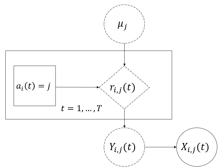
Figure 1: Graphical model for the hybrid mechanism $H_{i,j}$ of agent $i$.

We present two federated learning algorithms. The first, termed DP-Master-worker UCB algorithm, employs the DP mechanism to compute the individual arm index that consists of a private mean as well as an additional privacy-induced uncertainty. Then, the central node aggregates and returns back an aggregated index that will be used arm selection. The second, termed DP-Decentralized UCB algorithm, employs the same DP mechanism, but the agents estimate the index by averaging their neighbors’ input.

III-A DP-Master-worker UCB algorithm

In Algorithm 1, each arm $j$ of each agent $i$ uses the DP mechanisms $H_{i,j}$ (shown in Figure 1) to maintain a private total reward $s_{i,j}$. The communication phase begins when the counter $\eta=2^{p}~{}\text{for}~{}p=1,2,...$. The individual arm index of each agent $i$ is first updated using the private mean, the upper confidence bound and the additional noise due to privacy (Line 12). Then, the central node averages all the private indices to compute an average index which leads to the same best arm selection for all $M$ agents. Each agent $i$ starts from the common index and privately updates it. For each agent, if an arm is pulled for the $p^{th}$ time consecutively (without switching to any other arms in between), it will also be played for the next $2^{p}$ time slots.

Algorithm 1 DP-Master-worker UCB algorithm

1:Initialization: Set $t~{}=~{}0$ and counter $\eta~{}=~{}1$;

2:For each arm $j,~{}1\leq j\leq K$ of each agent $i,~{}1\leq i\leq M$, instantiate DP mechanisms $H_{i,j}$.

3:Input: The differential privacy parameter $\epsilon$;

4:while $t\leq T$ do

5:     for agent $i$ to $M$ do

6:         if $t\leq K$ then

7:              Play arm $a_{i}(t)=t$, observe reward $r_{i,a_{i}(t)}(t)$

8:              Insert $r_{i,a_{i}(t)}(t)$ to the DP mechanism $H_{i,a_{i}(t)}$

9:         end if

10:         if $\eta=2^{p}$ for $p=0,1,...$ then

11:              Update total reward $s_{i,j}(t)$ using $H_{i,j}$

12:              Update $\upsilon_{i,j}=\frac{1}{\epsilon}log\frac{1}{\delta}\log^{1.5}n_{i,j}(t)$

13:              Update index $I_{i,j}(t)=X_{i,j}+\sqrt{\frac{2\log t}{n_{i,j}(t)}}+\frac{\upsilon_{i,j}(t)}{n_{i,j}(t)}$

14:              /*Begin communication phase

15:              Send index $I_{i,j}(t)$ to the central node

16:              Receive the averaged index $I^{avg}_{j}(t)$ of $j$ arms

17:              /*End communication phase

18:              Pull best arm $a^{*}_{i}(t)={argmax}_{j}I^{avg}_{j}(t)$

19:              if $a^{*}_{i}(t)\neq a^{*}_{i}(t-1)$ then

20:                  Reset $\eta=1$;

21:              end if

22:         else

23:              $a^{*}_{i}(t)=a^{*}_{i}(t-1)$

24:         end if

25:         Play arm $a^{*}_{i}(t)$, observe the reward $r_{i,a^{*}_{i}(t)}(t)$

26:         Insert $r_{i,a^{*}_{i}(t)}(t)$ to the DP mechanism $H_{i,a^{*}(t)}$

27:         Update $t=t+1,\eta=\eta+1$

28:     end for

29:     for The central node do

30:         /*Begin communication phase

31:         Receive index sequence $\left\{I_{1,j}...I_{M,j}\right\}$ of $j$ arms

32:         Compute and return back $I^{avg}_{j}=\frac{1}{M}\sum_{i=1}^{M}I_{i,j}$

33:         /*End communication phase

34:     end for

35:end while

We next analyze the algorithm performance. Theorem 1 provides the privacy performance of Algorithm 1.

Lemma 1 (Privacy error bound).

The error between the empirical mean $Y_{i,j}$ and private mean $X_{i,j}$ after $n_{i,j}$ times of plays is bounded as $|Y_{i,j}-X_{i,j}|\leq h_{n_{i,j}}$ with probability at least $1-\delta$, where $h_{n_{i,j}}$ is the error incurred by the private mechanism calculated as $h_{n_{i,j}}=\frac{1}{\epsilon}\cdot\log^{1.5}({n_{i,j}})\cdot\log\frac{1}{\delta}\cdot\frac{1}{n_{i,j}}$.

Proof.

This follows directly from the Fact 1 (Appendix.A[19]) that the hybrid mechanism remains $(\epsilon,\delta)$-DP after any number $n_{i,j}$ of plays since each time only one arm is pulled, that will affect only one mechanism. ∎

Theorem 1 (Privacy of Algorithm 1).

Algorithm 1 is $\epsilon$- differential private after $T$ timeslots with $\delta=T^{-4}$.

Proof.

Proposition 2.1 of [6] proves the post-processing property of DP mechanisms: the composition of a mapping $f$ with an $(\epsilon,\delta)$- differentially private algorithm is also $(\epsilon,\delta)$ differentially private. Using Lemma 1, the hybrid mechanism is $(\epsilon,\delta)$- differentially private. Moreover, our Algorithm 1 can be seen as a mapping from the averaged output of the hybrid mechanism to the action. This completes our proof. ∎

Theorem 2 gives the regret of Algorithm 1. Here we only give a proof sketch, the complete proof can be found in Appendix.C[19].

Theorem 2 (Regret of Algorithm 1).

The learning regret of Algorithm 1 is

$$\begin{array}[]{ll}R^{C}(T)\leq MK\Delta_{max}(4+\max[(\frac{8\log{T}}{\epsilon(1-\beta_{0})\Delta_{min}})^{2.25},\left\lceil\frac{8\log{T}}{\Delta_{min}^{2}\beta_{0}^{2}}\right\rceil]\end{array}$$

for some $0<\beta_{0}<1$, where $\Delta_{max}=\max\left\{\Delta_{j}\right\}$, $\Delta_{min}=\min\left\{\Delta_{j}\right\}$, $\epsilon$ is the parameter for $(\epsilon,\delta)$ privacy, $\delta=T^{-4}$.

Proof outline. The regret incurred during the time horizon $T$ is caused by playing suboptimal arms. We first bound the amount of error between the private and empirical means that are caused by the DP mechanism. Using this bound and Lemma 1, we estimate the number of times that we play suboptimal arms. We show that after a sufficient number of times $O(\frac{MK\log^{1.5}T}{\epsilon\Delta^{2}_{min}})$, a suboptimal arm will not be selected with high probability.

Remark: Through the central mode we obtain $O(MK\log^{2.25}(T))$ regret. The DP mechanism mainly increases the exploration rounds. If we do not use the DP mechanism, the $O(\log^{2.25}T)$ term vanishes. We note that after $\frac{8\log T}{\Delta_{min}^{2}}$ plays, the suboptimal arms will be selected with low probability, and we can achieve a $O(MK\log T)$ regret. Note that in Theorem 2, the parameter $\epsilon$ reflects the trade off between privacy and regret, where the privacy increases as $\epsilon$ decrease.

III-B DP-Decentralized UCB algorithm

Algorithm 2 DP-Decentralized UCB algorithm

1:Initialization: Set $t=0$; $\hat{\mathbf{n}}_{j}(0)=\left\{\hat{n}_{1,j}(0),...,\hat{n}_{M,j}(0)\right\}$, $\hat{\mathbf{s}}_{j}(0)=\left\{\hat{s}_{1,j}(0),...,\hat{s}_{M,j}(0)\right\}$

2:For each arm $j,~{}1\leq j\leq K$ of each agent $i,~{}1\leq i\leq M$, instantiate DP Mechanisms $H_{i,j}$.

3:Input: The differential privacy parameter $\epsilon$; matrix $P$ represents the network structure; $\rho\geq 1$;

4:while $t\leq T$ do

5:     for agent $i$ to $M$ do

6:         if $t\leq K$ then

7:              play arm $a_{i}(t)=t$, observe the reward $r_{a_{i}(t)}(t)$

8:              Insert $r_{a_{i}(t)}(t)$ to the DP mechanism $H_{i,a_{i}(t)}$

9:         else

10:              /*Begin the communication phase

11:              Update the estimated play numbers:

12:              $\hat{\mathbf{n}}_{j}(t)=P\hat{\mathbf{n}}_{j}(t-1)+P\mathbf{\eta}_{j}(t-1)$

13:              Update the additional private error term:

14:              $\hat{\upsilon}_{j,j}(t)=\frac{1}{\epsilon}\log\frac{1}{\delta}\log^{1.5}\hat{n}_{i,j}(t)$

15:              Update the estimated total rewards:

16:              $\hat{\mathbf{s}}_{j}(t)=P{\hat{\mathbf{s}}}_{j}(t-1)$

17:              /*End the communication phase.

18:              Update the arm index :

19:              $I_{i,j}(t)=\hat{{X}}_{i,j}+\sqrt{2\rho\frac{\hat{n}_{i,j}(t)+c_{i}}{M\hat{n}_{i,j}(t)}\cdot\frac{\log t}{\hat{n}_{i,j}(t)}}+\frac{\hat{\upsilon}_{i,j}(t)}{\hat{n}_{i,k}(t)}$

20:              Select the best arm $a_{i}(t)={argmax}_{j}I_{i,j}(t)$

21:              Observe the reward $r_{a_{i}(t)}(t)$

22:              Insert $r_{a_{i}(t)}(t)$ to the DP mechanism $H_{i,a_{i}(t)}$

23:              Update $s_{i,a_{i}(t)}(t)$ using DP mechanism $H_{i,a_{i}(t)}$

24:              $t=t+1$

25:         end if

26:     end for

27:end while

In Algorithm 2, the agents average their model with their neighbors’ models at each time $t$, instead of aggregating their values with the help of a central node. We assume that each agent maintains a bi-directional communication with a set of neighboring agents. We consider Gaussian distributions for each arm’s reward, i.e., the reward at arm $j$ is sampled from a Gaussian distribution with mean $\mu_{i,j}$ and variance $\sigma^{2}$. We assume that the variance $\sigma^{2}$ is known and is the same at each arm. We use a consensus algorithm that captures the effect of the additional private information an agent receives through communication with other agents. We represent the network as a graph where nodes are agents and edges connect neighboring agents. A discrete-time consensus algorithm can be expressed as:

$$\mathbf{x}(t+1)=P\mathbf{x}(t),$$ (3)

where $x$ is the quantity we want the agents to agree on, and $P$ is a row stochastic matrix given by

$$P=\mathit{I}_{M}-\frac{\kappa}{d_{max}}L.$$ (4)

Here, $\mathit{I}_{M}$ is the identity matrix with order M, $d_{max}=\max_{i}\deg(i),i\in\left\{1,...,M\right\}$ and $\deg(i)$ is the degree of agent $i$. $\kappa\in[0,1]$ is a step size parameter and $L$ is the Laplacian matrix of this communication graph. Without loss of generality, we assume that the eigenvalues of $P$ are ordered as $\lambda_{1}=1\geq\lambda_{2}\geq...\geq\lambda_{M}\geq-1$.

For our federated private MAB problem, we use the following definitions, that are similar to the definitions in Algorithm 1. Let $\hat{s}_{i,j}$ be the estimated total private reward, $\hat{y}_{i,j}$ be the estimated total true reward of arm $j$ at agent $i$, and $\hat{n}_{i,j}$ be the estimated total number of times that the arm $j$ has been played by agent $i$. Let $\hat{{X}}_{i,j}={\hat{s}_{i,j}}/{\hat{n}_{i,j}}$ be the estimated private mean, and $\hat{{Y}}_{i,j}={\hat{y}_{i,j}}/{\hat{n}_{i,j}}$ be the estimated empirical mean.

Without taking into account differential privacy, the consensus algorithm will update $\hat{y}_{i,j}$ and $\hat{n}_{i,j}$ as follows:

$$\mathbf{\hat{n}}_{j}(t+1)=P\mathbf{\hat{n}}_{j}(t)+P\mathbf{\xi}_{j}(t)$$ (5)

$$\mathbf{\hat{y}}_{j}(t+1)=P\mathbf{\hat{y}}_{j}(t)+P\mathbf{r}_{j}(t),$$ (6)

where ${\xi}_{i,j}(t)=I(a_{i}(t)=j)$, indicating if arm $j$ is played by agent $i$ at time slot $t$; $r_{i,j}(t)$ is the reward with respect to the action which is generated by the distribution $N(\mu_{j},\sigma^{2})$. $\mathbf{\hat{n}}_{j}(t),\mathbf{\xi}_{j}(t),\mathbf{\hat{y}}_{j}(t),\mathbf{r}_{j}(t)$ are vectors that connect the values $\hat{n}_{i,j}(t),\xi_{i,j}(t),\hat{y}_{i,j}(t),r_{i,j}(t)$ for $i=1,...,M$ respectively. We note that under our DP mechanism, an agent can not observe the reward sequences. Thus, we use the following equation to update the private total rewards instead of (6):

$$\mathbf{\hat{s}}_{j}(t+1)=P\mathbf{\hat{s}}_{j}(t).$$ (7)

The above equation captures the fact that only the private total reward $\mathbf{\hat{s}}_{j}(t)$ can be broadcasted through the network graph, not $\mathbf{r}_{j}(t)$. We still keep (5) because we only aim to keep the reward values private and not the numbers $\mathbf{\hat{n}}_{j}$.

Each arm $j$ of each agent $i$ uses the analogous DP mechanisms $H_{i,j}$ in the the Algorithm 1 to maintain a private total reward. The communication phase occurs at each timeslot to update the estimate play numbers $\hat{n}_{i,j}(t)$ and the total reward $\hat{s}_{i,j}(t)$ using (5) (7). Agent $i$ selects the arm with the maximum index denoted as:

$$I_{i,j}(t)=\hat{{X}}_{i,j}+\sqrt{2\rho\frac{\hat{n}_{i,j}(t)+c_{i}}{M\hat{n}_{i,j}(t)}\cdot\frac{\log t}{\hat{n}_{i,j}(t)}}+\frac{\hat{\upsilon}_{i,j}(t)}{\hat{n}_{i,k}(t)},$$ (8)

where $c_{0},c_{i}$ are parameters representing the network stricture and $\rho>1$ is the exploration parameter. From (8) we notice that the estimation performance, the network structure, and the exploration parameter, all affect the learning performance.

Theorem 3 (Privacy of Algorithm 2).

Algorithm 2 is $(\epsilon,\delta)$- differentially private after $T$ timeslots with $\delta=\frac{1}{2}T^{-\rho}$.

The proof of Theorem 3 is similar to that of Theorem 1.

Theorem 4 (Regret of Algorithm 2).

The learning regret of Algorithm 2 is

$$\begin{array}[]{ll}R^{D}(T)\leq\frac{2MK\rho\Delta_{max}}{\rho-1}+\sum_{i=1}^{M}\sum_{j>1}^{K}\max[(\frac{2+2\rho\log{T}}{\epsilon(1-\beta_{0})})^{2.25},\\ \left\lceil\frac{c_{0}}{\beta_{0}^{2}}+\frac{8\sigma^{2}\rho(1+c_{i})\log T}{\beta_{0}^{2}\Delta_{j}}\right\rceil]\end{array}$$

for some $0<\beta_{0}<1,~{}\rho\geq 1$, where $\Delta_{max}=\max\left\{\Delta_{j}\right\}$, $\Delta_{min}=\min\left\{\Delta_{j}\right\}$ and $\epsilon$ is the parameter for $(\epsilon,\delta)$ privacy, $\delta=\frac{1}{2}T^{-\rho}$ and $c_{i}$, $c_{0}$ are parameters of the network graph.

Proof outline. The regret is mainly caused by the estimated variance due to communication and the privacy requirements. By using Lemma 1 and Lemma 2 (provided in Appendix.B[19]), we first bound the amount of error between the estimated private mean and empirical mean. We note that the communication cost is also reflected in this bound. Using this bound, we estimate the number of times suboptimal arms are selected, and complete the proof. The complete proof can be found in Appendix.D[19].

Remark: From Theorem 4 we obtain $O(MK\log^{2.25}T)$ regret. Both the communication and the privacy mechanism result in an expansion of the exploration phase. The DP mechanism leads to an additional $O(\log^{2.25}T)$ regret with the parameter $\epsilon$ inversely proportional to the regret. The federated learning setup introduces constants $c_{0}$ and $c_{i}$ into the regret which depend on the network topology. In particular, $c_{0}$ is proportional to the network scale and $c_{i}$ depends on the number of neighbors of agent $i$. The sparser the network connection, the larger the $c_{i}$ and the regret. A larger exploration parameter $\rho$ also implies more exploration rounds.

IV Experiments

In this section, we mainly perform numerical simulations to verify and analyze the performance of Algorithm 2. We choose $M=20$ and $K=10$. The 20 agents are connected according to a cycle graph which is a fully decentralized setting. Figure 1 shows the impact of varying the privacy parameter $\epsilon$ in $\{1.5,2,5\}$ with fixed $\rho=2$. We can see that the regret increases with $\epsilon$. Figure 2 shows the impact of varing the exploration parameter $\rho$ in $\{1.2,2,4\}$ with fixed $\epsilon=2$. Again as expected the regret increases with $\rho$. These results demonstrate the tradeoff between the regret (recommendation accuracy) and privacy.

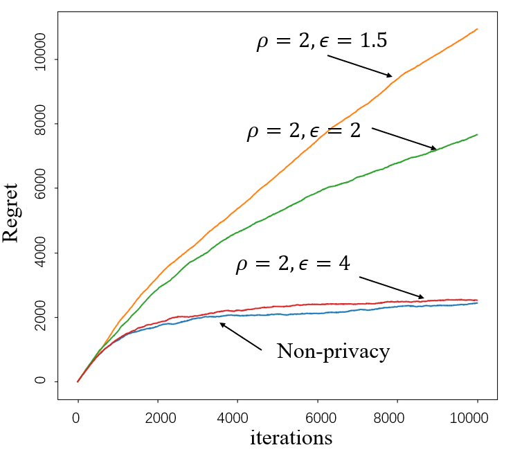
(a) Regret as a function privacy parameter $\epsilon$.

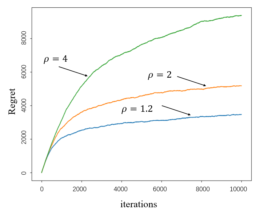
(b) Regret as a function of exploration parameter $\rho$.

Figure 2: Regret performance of Algorithm 2.

V Conclusion

In this paper, we proposed a distributed MAB framework for recommendation systems that incorporates differential privacy. At each distributed agent, we use an ($\epsilon,\delta$) differentially private variant of UCB scheme to ensure that agents do not reveal information on the reward values. We designed algorithms for two multi-agent settings: the DP-Master-worker UCB algorithm and the DP-Decentralized UCB algorithm each capturing a different communication network connecting agents. We analyzed both the privacy and regret performance and showed how the need for communication and privacy can influence the decision making performance of the agents.

VI Appendix

VI-A Useful facts

Fact 1 (Hybrid Mechanism, Corollary 4.8 in [18]) The hybrid mechanism is $\epsilon$- differential private and has an error bounded with probability at least $1-\delta$ by $\frac{1}{\epsilon}\cdot(\log~{}t)^{1.5}\cdot\log\frac{1}{\delta}$ at time $t$.

Fact 2 (Chernoff-Hoeffding bound) Let $X_{1},...,X_{t}$ be a sequence of real-valued random variables with common range $[0,1]$, and such that $\mathbb{E}[X_{t}|X_{1},...,X_{t-1}]=\mu$. Let $S_{t}=\sum_{i=1}^{t}X_{t}$. Then for all $a\geq 0$,

$$P(S_{t}\geq t\mu~{}+~{}a)~{}\leq~{}e^{-2a^{2}/t},P(S_{t}\leq t\mu~{}+~{}a)~{}\leq~{}e^{-2a^{2}/t}$$

VI-B Lemmas

Lemma 2 (Estimated Performance of Algorithm 2).

i) The estimated number of plays satisfies:

$$n_{j}^{\text{avg}}(t)-c_{0}\leq\hat{n}_{i,j}(t)\leq n_{j}^{\text{avg}}(t)+c_{0};$$

ii) $\hat{{Y}}_{i,j}$ is an unbiased estimation with $\mathbb{E}[\hat{{Y}}_{i,j}(t)]=\mu_{j}$;
iii) The variance of $\hat{{Y}}_{i,j}(t)$ is bounded by :

$$\text{Var}[\hat{{Y}}_{i,j}(t)]\leq\frac{\hat{n}_{i,j}(t)+c_{i}}{M\hat{n}_{i,j}(t)^{2}}\sigma^{2};$$

iv) The error between $\hat{{Y}}_{i,j}(t)$ and $\hat{{X}}_{i,j}(t)$ can be bounded by:

$$h_{\hat{n}_{i,j}(t)}=\frac{1}{\epsilon}\cdot\log^{1.5}({\hat{n}_{i,j}})\cdot\log\frac{1}{\delta}\cdot\frac{1}{\hat{n}_{i,j}}$$

where $n_{i,j}^{\text{avg}}(t)=\frac{1}{M}\sum_{\tau=1}^{t}\mathbf{1}_{M}^{T}\mathbf{\xi}_{j}(\tau)$ is the total number of times arm $j$ has been pulled by agent $i$ up to time $t$.

Proof.

Let $\lambda_{j}$ be the $j$ th largest eigenvalue of $P$, $\mathbf{u}_{j}$ be the eigenvector corresponding to $\lambda_{j}$.

Then we have $\lambda_{1}=1$ and $\mathbf{u}_{1}=\mathbf{1}_{M}/\sqrt{M}$. We define

$$\nu_{pk}^{+sum}=\sum_{d=1}^{M}u_{p}^{d}u_{k}^{d}\mathbbm{1}((\mathbf{u}_{p}\mathbf{u}_{k}^{\top})_{ii}\geq 0)$$ (9)

$$\nu_{pk}^{-sum}=\sum_{d=1}^{M}u_{p}^{d}u_{k}^{d}\mathbbm{1}((\mathbf{u}_{p}\mathbf{u}_{k}^{\top})_{ii}\leq 0)$$ (10)

To present the topology of communication graph, we denote two parameters $c_{0}$ and $c_{i}$ as:

$$c_{0} = \sqrt{M}\sum_{p=2}^{M}\frac{|\lambda_{p}|}{1-|\lambda_{p}|}$$ (11)

$$c_{i} = M\sum_{p=1}^{M}\sum_{k=2}^{M}\frac{|\lambda_{p}||\lambda_{k}|}{1-|\lambda_{p}||\lambda_{k}|}a_{pk}(i)$$ (12)

Where

$$a_{pk}(i)=\left\{\begin{matrix}\nu_{pk}^{+sum}(\mathbf{u}_{p}\mathbf{u}_{k}^{\top})_{kk}~{},\text{if}~{}\lambda_{p}\lambda_{k}\geq 0~{}\&~{}(\mathbf{u}_{p}\mathbf{u}_{k}^{\top})_{ii}\geq 0\\ \nu_{pk}^{-sum}(\mathbf{u}_{p}\mathbf{u}_{k}^{\top})_{ii}~{},\text{if}~{}\lambda_{p}\lambda_{k}\geq 0~{}\&~{}(\mathbf{u}_{p}\mathbf{u}_{k}^{\top})_{ii}\leq 0\\ \max\left\{|\nu_{pk}^{-sum}|,\nu_{pk}^{+sum}\right\},\text{if}~{}\lambda_{p}\lambda_{k}<0\end{matrix}\right.$$

We start with the first statement. From (5) it follows that,

$$\hat{\mathbf{n}}_{j}(t) = P^{t}\hat{\mathbf{n}}_{j}(0)+\sum_{\tau=0}^{t-1}P^{t-\tau}\mathbb{\xi}_{j}(\tau)$$ (13)

$$= \sum_{\tau=0}^{t-1}[\frac{1}{M}\mathbf{1}_{M}\mathbf{1}_{M}^{\top}\mathbb{\xi}_{j}(\tau)+\sum_{p=2}^{M}\lambda_{p}^{t-\tau}\mathbf{u}_{p}\mathbf{u}_{p}^{\top}\mathbb{\xi}_{j}(\tau)]$$

$$= n_{j}^{\text{avg}}(t)\mathbf{1}_{M}+\sum_{\tau=0}^{t-1}\sum_{p=2}^{M}\lambda_{p}^{t-\tau}\mathbf{u}_{p}\mathbf{u}_{p}^{\top}\mathbb{\xi}_{j}(\tau)$$

We now bound the second term on the right hand of (13):

$$\sum_{\tau=0}^{t-1}\sum_{p=2}^{M}\lambda_{p}^{t-\tau}\mathbf{u}_{p}\mathbf{u}_{p}^{\top}\mathbb{\xi}_{j}(\tau)\leq\sum_{\tau=0}^{t-1}\sum_{p=2}^{M}|\lambda_{p}^{t-\tau}|\left\|\mathbf{u}_{p}\right\|_{2}^{2}\left\|\mathbb{\xi}_{j}(\tau)\right\|_{2}$$

$$\leq\sqrt{M}\sum_{\tau=0}^{t-1}\sum_{p=2}^{M}|\lambda_{p}^{t-\tau}|\leq c_{0}$$ (14)

This complete the statement i).

Similarly, for statement ii) we have:

$$\hat{\mathbf{y}}_{j}(t)=P^{t}\hat{\mathbf{s}}_{j}(0)+\sum_{\tau=0}^{t-1}P^{t-\tau}\mathbf{r}_{j}(\tau)=\sum_{\tau=0}^{t-1}=P^{t-\tau}\mathbf{r}_{j}(\tau)$$ (15)

Calculate expected on both side of above equality we have $\mathbb{E}[\hat{\mathbf{y}}_{j}(t)]=\mu_{j}\sum_{\tau=0}^{t-1}\mathbb{\xi}_{j}(\tau)=\mu_{i}\hat{\mathbf{n}}_{j}(t)$, this proof statement ii).

For the third statement, we have

$$\text{Cov}[\hat{\mathbf{y}}_{j}(t)] = (P^{t-\tau})\Sigma(\tau)\Sigma(\tau)^{\top}(P^{t-\tau})^{\top}$$ (16)

$$= \sum_{\tau=0}^{t-1}\sum_{p=1}^{M}\sum_{k=1}^{M}\lambda_{p}^{t-\tau}\lambda_{j}^{t-\tau}\mathbf{u}_{p}\mathbf{u}_{p}^{\top}\Sigma(\tau)\Sigma(\tau)^{\top}\mathbf{u}_{k}\mathbf{u}_{k}^{\top}$$

$$= \underset{①}{\underbrace{\sigma^{2}\sum_{\tau=0}^{t-1}\sum_{p=1}^{M}\sum_{k=1}^{M}(\lambda_{p}\lambda_{k})^{t-\tau}\varsigma_{pk}(\tau)(\mathbf{u}_{p}\mathbf{u}_{k}^{\top})}}$$

$$+ \underset{②}{\underbrace{\frac{1}{M}\sum_{\tau=0}^{t-1}\sum_{p=1}^{M}\lambda_{p}^{t-\tau}\mathbf{u}_{p}\mathbf{u}_{k}^{\top}\Sigma(\tau)\Sigma(\tau)^{\top}\mathbf{1}_{M}\mathbf{1}_{M}^{\top}}}$$

Where $\Sigma(\tau)=\sigma\text{diag}(\mathbb{\xi}_{j}(\tau))$, $\varsigma_{pk}(\tau)=\mathbf{u}_{p}^{\top}\text{diag}(\mathbb{\xi}_{j}(\tau))\mathbf{u}_{k}$. We examine the $ii-$th entry of (16) and define ① and ② as the $ii$-th entry of the first term and second term in (16) respectively.

$$① \leq \sigma^{2}\sum_{\tau=0}^{t-1}\sum_{p=1}^{M}\sum_{k=1}^{M}|\lambda_{p}\lambda_{k}|^{t-\tau}|\varsigma_{pk}(\tau)(\mathbf{u}_{p}\mathbf{u}_{k}^{\top})_{ii}|$$ (17)

$$\leq \sigma^{2}\sum_{\tau=0}^{t-1}\sum_{p=1}^{M}\sum_{k=1}^{M}|\lambda_{p}\lambda_{k}|^{t-\tau}|a_{pk}(i)$$

$$\leq \sum_{p=1}^{M}\sum_{k=2}^{M}\frac{|\lambda_{p}||\lambda_{k}|}{1-|\lambda_{p}||\lambda_{k}|}a_{pk}(i)=\sigma^{2}\frac{c_{i}}{M}$$

$$②=\frac{1}{M}[(\sum_{\tau=0}^{t-1}\sum_{p=1}^{M}\lambda_{p}^{t-\tau}\mathbf{u}_{p}\mathbf{u}_{k}^{\top}\mathbf{\xi}_{j}(\tau))\mathbf{1}_{M}^{\top}]_{ii}=\sigma^{2}\frac{\hat{n}_{i,j}(t)}{M}$$ (18)

Combining (17) and (18), we establish statement iii).

Directly following Lemma 1, we can proof statement iv). This complete the proof of Lemma 2. ∎

VI-C Proof of Theorem 2

Proof.

Using Lemma 1, we rewrite the bound into following equations:

$$P(X\geq Y+h_{n})\leq\delta$$ (19)

$$P(X\leq Y-h_{n})\leq\delta$$ (20)

Recall $\epsilon$ is the is the differential privacy parameter. The regret incurred during time horizon $T$ can be analyzed as the sum of the regret caused by playing suboptimal arms and recomputing the arm index by federated learning. We denote $n_{i,j}(T)$ as the times that a suboptimal arm $j$ is played by agent $i$, $c_{t,n}=\sqrt{\frac{\log T}{2}}$ as the UCB confidence index. Our proof steps mostly follows the demonstration of UCB algorithm[9]. Considering a suboptimal arm $j\geq 1$ of player $i$, let $\tau_{i,j}(m)$ be the time that play make the $m$-th switch to arm $j$ and $\tau^{\prime}_{i,j}(m)$ be the time that the player leave arm $j$ and turn another one. Then, we have,

$$\begin{array}[]{ll}n_{i,j}(T)\\ \leq 1+\sum_{m=1}^{T}\left|\tau^{\prime}_{i,j}(m)-\tau_{i,j}(m)\right|I\left\{\text{Play arm}~{}j~{}\text{at time~{}}\tau_{i,j}(m)\right\}\\ \leq 1+\sum_{m=1}^{T}\left|\tau^{\prime}_{i,j}(m)-\tau_{i,j}(m)\right|\\ I\left\{\sum_{i=1}^{M}I_{i,j}(\tau_{i,j}(m)-1)\geq\sum_{i=1}^{M}I_{i,1}(\tau_{i,j}(m)-1)\right\}\\ \leq l+\sum_{m=1}^{T}\sum_{l=0}^{\infty}2^{p}I\left\{{\sum_{i=1}^{M}I_{i,j}(\tau_{i,j}(m)+2^{p}-2)\geq}\right.\\ \phantom{}\left.{\sum_{i=1}^{M}I_{i,1}(\tau_{i,j}(m)+2^{p}-2),n_{i,j}(\tau_{i,j}(m)-1)\geq l}\right\}\\ \leq l+\sum_{m=1}^{T}\sum_{p=0}^{\infty}2^{p}I\left\{{\sum_{i=1}^{M}I_{i,j}(m+2^{p}-2)\geq}\right.\\ \phantom{}\left.{\sum_{i=1}^{M}I_{i,1}(m+2^{p}-2),n_{i,j}(m-1)\geq l}\right\}\\ \leq l+\sum_{m=1}^{\infty}\sum_{m+2^{p}\leq T}\leq 2^{p}\sum_{n_{i,1}=1}^{m+2^{p}}\sum_{n_{i,j}=l}^{m+2^{p}}\\ I\left\{{\sum_{i=1}^{M}({X}_{i,j}(m+2^{p})+c_{m+2^{p},n_{i,j}}+h_{n_{i,j}})\geq}\right.\\ \phantom{}\left.{\sum_{i=1}^{M}({X}_{i,1}(m+2^{p})+c_{m+2^{p},n_{i,1}}+h_{n_{i,1}})}\right\}\end{array}$$

In Algorithm 1, if an arm is for the pth time consecutively (without switching to any other arms in between), it will be played for the next $2^{p}$ slots. The second inequality uses this fact. In the second last inequality , we replace $\tau_{i,j}(m)$ by $m$ which is clearly an upper bound.

It should be noted that each time step $t$ when index updates, we have $I_{1,j}(t)=I_{2,j}(t)=...=I_{i,j}(t)=...=I_{M,j}(t)=\frac{1}{M}\sum_{i=1}^{M}I_{i,k}(t)$. That means all agents select the same arm according to the central update results, so in equation (VI-C), we can observe that the event $\sum_{i=1}^{M}({X}_{i,j}(m+2^{p})+c_{m+2^{p},n_{i,j}}+h_{n_{i,j}})\geq\sum_{i=1}^{M}({X}_{i,1}(m+2^{p})+c_{m+2^{p},n_{i,1}}+h_{n_{i,1}})$ implies that for each player $i$ at least one of the following events holds:

$${X}_{i,1}(m+2^{p})\leq\mu_{i,1}-c_{m+2^{p},n_{i,1}}-h_{n_{i,1}}$$ (21)

$${X}_{i,j}(m+2^{p})\geq\mu_{i,j}+c_{m+2^{p},n_{i,j}}+h_{n_{i,j}}$$ (22)

$$\mu_{i,1}\leq\mu_{i,j}+2c_{m+2^{p},n_{i,j}}+2h_{n_{i,j}}$$ (23)

Now, using the Chernoff-Hoeffding bound, we can get:

$$\Pr(\eqref{ev1}) = \Pr({X}_{i,1}(m+2^{p})\leq\mu_{i,1}-c_{m+2^{p},n_{i,1}}-h_{n_{i,1}})$$ (24)

$$= \Pr({X}_{i,1}(m+2^{p})\leq{Y}_{i,1}(m+2^{p})-h_{n_{i,1}}$$

$$\vee {Y}_{i,1}(m+2^{p})\leq\mu_{i,1}-c_{m+2^{p},n_{i,1}})$$

$$= \Pr({X}_{i,1}(m+2^{p})\leq{Y}_{i,1}(m+2^{p})-h_{n_{i,1}})$$

$$+ \Pr({Y}_{i,1}(m+2^{p})\leq\mu_{i,1}-c_{m+2^{p},n_{i,1}})$$

$$= \delta+(m+2^{p})^{-4}$$

Similarly, we can use (19) and the Chernoff-Hoeffding bound to prove a bound on (22):

$$\Pr(\eqref{ev2}) = \Pr({X}_{i,j}(m+2^{p})\geq\mu_{i,1}+c_{m+2^{p},n_{i,j}}+h_{n_{i,j}})$$ (25)

$$= \Pr({X}_{i,j}(m+2^{p})\leq{Y}(m+2^{p})_{i,j}+h_{n_{i,1}}$$

$$\vee {Y}_{i,j}(m+2^{p})\leq\mu_{i,j}+c_{m+2^{p},n_{i,j}})$$

$$= Pr({X}_{i,j}(m+2^{p})\leq{Y}_{i,j}(m+2^{p})+h_{n_{i,j}})$$

$$+ \Pr({Y}_{i,j}(m+2^{p})\leq\mu_{i,j}-c_{m+2^{p},n_{i,j}})$$

$$= \delta+(m+2^{p})^{-4}$$

To prove a bound on (23), we try to find a minimum number $n_{i,j}$ for which (23) is always false. This event is flase indicates that $\Delta_{i,j}\geq 2c_{m+2^{p},n_{i,j}}+2h_{n_{i,j}}$, which implies the following two equations hold for any $0\leq\beta_{0}\leq 1$.

$$\beta_{0}\Delta_{i,j}\geq 2c_{m+2^{p},n_{i,j}}$$ (26)

$$(1-\beta_{0})\Delta_{i,j}\geq 2h_{n_{i,j}}$$ (27)

For $n_{i,j}\geq\left\lceil\frac{8\log T}{\Delta_{i,j}^{2}\beta_{0}^{2}}\right\rceil$, (26) is false. Equation $\eqref{ev5}$ implies that

$$n_{i,j}\geq\beta_{1}\cdot\log(n_{i,j})^{1.5}$$ (28)

where

$$\beta_{1}=\frac{2}{(1-\beta_{0})\Delta_{i,j}}\cdot\frac{1}{\epsilon}\log{\frac{1}{\delta}}$$ (29)

Let $x=-\log(n_{i,j}/1.5)$, above inequality can be rewrite in the standard transcendental algebraic inequality form:

$$e^{-x}\geq-1.5x\beta_{1}^{\frac{1}{1.5}}$$ (30)

The solution can be given by the Lambert W function, so

$$n_{i,j} \geq \exp(-1.5(W(-1,\frac{-1}{1.5\beta_{1}^{\frac{1}{1.5}}})))$$ (31)

$$\approx \beta_{1}^{2.25}=(\frac{2}{(1-\beta_{0})\Delta_{i,j}}\cdot\frac{1}{\epsilon}\log{\frac{1}{\delta}})^{2.25}$$

Here we choose $\delta=(m+2^{p})^{-4}\leq T^{-4}$,that yields

$$n_{i,j}\geq\max[(\frac{8}{(1-\beta_{0})\Delta_{i,j}}\cdot\frac{1}{\epsilon}\log{T})^{2.25},\frac{8\log T}{\Delta_{i,j}^{2}\beta_{0}^{2}}]$$ (32)

In summary, the total number of suboptimal plays is

$$\begin{array}[]{ll}\mathbb{E}[n(T)]=\sum_{i=1}^{M}\sum_{j>1}^{K}\mathbb{E}[n_{i,j}(T)]\\ =\sum_{i=1}^{M}\sum_{j>1}^{K}[\max[(\frac{8}{(1-\beta_{0})\Delta_{i,j}}\cdot\frac{1}{\epsilon}\log T)^{2.25},\phantom{}\left\lceil\frac{8\log T}{\Delta_{i,j}^{2}\beta_{0}^{2}}\right\rceil]]\\ +\sum_{m=1}^{\infty}\sum_{p=0}^{\infty}2^{p}\sum_{n_{i,1}=1}^{m+2^{p}}\sum_{n_{i,j}=1}^{m+2^{p}}4(m+2^{p})^{-4}\\ \leq\sum_{i=1}^{M}\sum_{j>1}^{K}(4+\max[(\frac{8}{(1-\beta_{0})\Delta_{i,j}}\cdot\frac{1}{\epsilon}\log T)^{2.25},\phantom{}\left\lceil\frac{8\log T}{\Delta_{i,j}^{2}\beta_{0}^{2}}\right\rceil])\\ \leq MK(4+\max[(\frac{8}{(1-\beta_{0})\Delta_{i,j}}\cdot\frac{1}{\epsilon}\log T)^{2.25},\phantom{}\left\lceil\frac{8\log T}{\Delta_{i,j}^{2}\beta_{0}^{2}}\right\rceil])\end{array}$$

The expected regret is

$$R^{C}(T)\leq\Delta_{max}\mathbb{E}(n(T))$$

$$\leq\Delta_{max}MK(4+\max[(\frac{8}{(1-\beta_{0})\Delta_{i,j}}\cdot\phantom{}\left\lceil\frac{8\log T}{\Delta_{i,j}^{2}\beta_{0}^{2}}\right\rceil])$$ (33)

This completes the proof. ∎

VI-D Proof of Theorem 4

Proof.

The proof is similar to Theorem 2. The regret incurred can be analyzed by playing the suboptimal arms ($j\geq 1$) during time horizon $T$:

$$\begin{array}[]{ll}n(T)=1+\sum_{i=1}^{M}\sum_{t=K+1}^{T}n_{i,j}(t)\\ =1+\sum_{i=1}^{M}\sum_{t=1}^{T}I\{a_{i}(t)=j\}\\ \leq l+\sum_{i=1}^{M}\sum_{t=1}^{T}I\{I_{i,j}(t)\geq I_{i,1}(t),n_{j}^{\text{avg}}\geq l\}\\ \leq l+\sum_{t=1}^{T}I\left\{{\sum_{i=1}^{M}\hat{{X}}_{i,j}(t)+c_{t,n_{i,j}}+h_{n_{i,j}}}\right.\\ \phantom{}\left.{\geq\sum_{i=1}^{M}\hat{{X}}_{i,1}(t)+c_{t,n_{i,1}}+h_{n_{i,1}},n_{j}^{\text{avg}}\geq l}\right\}\end{array}$$

At time slot $t$, the individual agent $i$ will choose a suboptimal arm only if the event $\left\{{\sum_{i=1}^{M}\hat{{X}}_{i,j}(t)+c_{t,\hat{n}_{i,j}+h_{\hat{n}_{i,j}}}\geq\sum_{i=1}^{M}\hat{{X}}_{i,1}(t)+c_{t,\hat{n}_{i,1}+h_{\hat{n}_{i,1}}}}\right\}$ holds. It indicated that at least one of the following three conditions must holds:

$$\hat{{X}}_{i,1}\leq\mu_{1}-c_{t,\hat{n}_{i,1}}-h_{\hat{n}_{i,1}}$$ (34)

$$\hat{{X}}_{i,j}\leq\mu_{j}+c_{t,\hat{n}_{i,j}}+h_{\hat{n}_{i,j}}$$ (35)

$$\mu_{1}<\mu_{j}+2c_{t,\hat{n}_{i},j}+2h_{\hat{n}_{i,j}}$$ (36)

According to Lemma 2, $c_{t,\hat{n}_{i,j}}=\sigma\sqrt{\frac{\hat{n}_{i,j}(t)+c_{i}}{M\hat{n}_{i,j}(t)}\cdot\frac{2\rho\log T}{\hat{n}_{i,j}(t)}}$. Using the Fact 2, the union bound and the Chernoff-Hoffding bound, we can prove the probability of (34) is:

$$\Pr(\eqref{ev6}) = Pr(\hat{{X}}_{i,1}\leq\mu_{1}-c_{t,\hat{n}_{i,1}}-h_{\hat{n}_{i,1}})$$ (37)

$$= \Pr(\hat{{X}}_{i,1}\leq\hat{{Y}}_{i,1}-h_{n_{i,1}})+$$

$$\Pr\left(z\geq\frac{\mathbb{E}[\hat{{Y}}_{i,1}]+c_{t,\hat{n}_{i,1}}-\mu_{1}}{\sqrt{\text{Var}(\hat{{Y}}_{i,1})}}\right)$$

$$\leq \delta+\Pr(z\geq\frac{c_{t,\hat{n}_{i,1}}}{\sqrt{\text{Var}(\hat{{Y}}_{i,1})}})$$

$$\leq \delta+\frac{1}{2}\exp(-\frac{c_{t,\hat{n}_{i,1}^{2}}}{2\text{Var}(\hat{{Y}}_{i,1})})\leq\delta+\frac{1}{2t^{\rho}}$$

where $z$ is the standard Gaussian random variable. The last inequality follows from the tail bounds for the error function and the statement ii) of Lemma 2. Similarly, we can prove the bound of event (35):

$$\Pr(\eqref{ev7})\leq\delta+\frac{1}{2t^{\rho}}$$ (38)

We can choose $\delta=\frac{1}{2t^{\rho}}$, which leading to :

$$\Pr(\eqref{ev6})\leq t^{-\rho}$$ (39)

$$\Pr(\eqref{ev7})\leq t^{-\rho}$$ (40)

To prove a bound on (36), we try to find a minimum number $\hat{n}_{i,j}$ for which (36) is always false. This event is false indicates that $\Delta_{i,j}\geq 2c_{t,n_{i,j}}+2h_{n_{i,j}}$, which implies the following two equations hold for any $0\leq\beta_{0}\leq 1$.

$$\beta_{0}\Delta_{i,j}\geq 2c_{t,\hat{n}_{i,j}}$$ (41)

$$(1-\beta_{0})\Delta_{i,j}\geq 2h_{\hat{n}_{i,j}}$$ (42)

For $l=\left\lceil\frac{c_{0}}{\beta_{0}^{2}}+\frac{8\sigma^{2}\rho(1+c_{i})\log T}{M\beta_{0}^{2}\Delta_{i,j}^{2}}\right\rceil$, (41) is false.

The appropriate choice of $n_{i,j}$ for holding $\eqref{ev12}$ can be same of Theorem 2 since (42) is only related to the DP error.

$$\hat{n}_{i,j} \geq \beta_{1}^{2.25}=(\frac{2}{(1-\beta_{0})\Delta_{i,j}}\cdot\frac{1}{\epsilon}\log{\frac{1}{\delta}})^{2.25}$$ (43)

Since we choose $\delta=\frac{1}{2}t^{-\rho}$,that yields

$$\begin{array}[]{ll}\hat{n}_{i,j}\geq\max[(\frac{2+2\rho\log T}{\epsilon(1-\beta_{0})\Delta_{i,j}})^{2.25},\phantom{}\left\lceil\frac{c_{0}}{\beta_{0}^{2}}+\frac{8\sigma^{2}\rho(1+c_{i})\log T}{M\beta_{0}^{2}\Delta_{i,j}^{2}}\right\rceil]\end{array}$$ (44)

In summary, the total number of suboptimal plays is

$$\begin{array}[]{ll}\mathbb{E}[n(T)]=\\ \sum_{i=1}^{M}\sum_{j>1}^{K}[\max[(\frac{2+2\rho\log T}{\epsilon(1-\beta_{0})\Delta_{i,j}})^{2.25},\phantom{}\left\lceil\frac{c_{0}}{\beta_{0}^{2}}+\frac{8\sigma^{2}\rho(1+c_{i})\log T}{M\beta_{0}\Delta_{i,j}^{2}}\right\rceil]]\\ \phantom{}+\sum_{t=1}^{T}\sum_{n_{i,1}=1}^{t}\sum_{n_{i,j}=1}^{t}2t^{-\rho}\\ \leq\sum_{i=1}^{M}\sum_{j>1}^{K}(\frac{2\rho}{\rho-1}+\max[(\frac{2+2\rho\log T}{\epsilon(1-\beta_{0})\Delta_{i,j}})^{2.25},\phantom{}\left\lceil\frac{c_{0}}{\beta_{0}^{2}}+\frac{8\sigma^{2}\rho(1+c_{i})\log T}{M\beta_{0}\Delta_{i,j}^{2}}\right\rceil])\\ \leq\frac{2MK\rho}{\rho-1}+\sum_{i=1}^{M}\sum_{j>1}^{K}\max[(\frac{2+2\rho\log T}{\epsilon(1-\beta_{0})\Delta_{i,j}})^{2.25},\phantom{}\left\lceil\frac{c_{0}}{\beta_{0}^{2}}+\frac{8\sigma^{2}\rho(1+c_{i})\log T}{M\beta_{0}^{2}\Delta_{i,j}^{2}}\right\rceil]\end{array}$$

Using $R^{D}(T)=\Delta_{max}\cdot\mathbb{E}[n(T)]$, we can complete the proof. ∎

References

• [1] M. Brodie, “The promise of distributed computing and the challenges of legacy information systems,” 12 1998.
• [2] L. Song and C. Fragouli, “Making recommendations bandwidth aware,” in IEEE Int. Symp. Inf. Theory (ISIT).   IEEE, 2017, pp. 2243–2247.
• [3] L. Song, C. Fragouli, and D. Shah, “Recommender systems over wireless: Challenges and opportunities,” Proc. IEEE Inf. Theory Workshop (ITW), 2018.
• [4] L. Song, C. Fragouli, and D. Shah, “Interactions between learning and broadcasting in wireless recommendation systems,” in 2019 IEEE International Symposium on Information Theory (ISIT), July 2019, pp. 2549–2553.
• [5] J. Konečnỳ, H. B. McMahan, F. X. Yu, P. Richtárik, A. T. Suresh, and D. Bacon, “Federated learning: Strategies for improving communication efficiency,” arXiv preprint arXiv:1610.05492, 2016.
• [6] C. Dwork, A. Roth et al., “The algorithmic foundations of differential privacy,” Foundations and Trends® in Theoretical Computer Science, vol. 9, no. 3–4, pp. 211–407, 2014.
• [7] L. Li, W. Chu, J. Langford, and R. E. Schapire, “A contextual-bandit approach to personalized news article recommendation,” in Proceedings of the 19th international conference on World wide web.   ACM, 2010, pp. 661–670.
• [8] C. Zeng, Q. Wang, S. Mokhtari, and T. Li, “Online context-aware recommendation with time varying multi-armed bandit,” in Proceedings of the 22nd ACM SIGKDD international conference on Knowledge discovery and data mining.   ACM, 2016, pp. 2025–2034.
• [9] P. Auer, N. Cesa-Bianchi, and P. Fischer, “Finite-time analysis of the multiarmed bandit problem,” Machine learning, vol. 47, no. 2-3, pp. 235–256, 2002.
• [10] S. Agrawal and N. Goyal, “Analysis of thompson sampling for the multi-armed bandit problem,” in Conference on Learning Theory, 2012, pp. 39–1.
• [11] K. Liu and Q. Zhao, “Distributed learning in multi-armed bandit with multiple players,” IEEE Transactions on Signal Processing, vol. 58, no. 11, pp. 5667–5681, Nov 2010.
• [12] D. Kalathil, N. Nayyar, and R. Jain, “Decentralized learning for multiplayer multiarmed bandits,” IEEE Transactions on Information Theory, vol. 60, no. 4, pp. 2331–2345, April 2014.
• [13] J. Rosenski, O. Shamir, and L. Szlak, “Multi-player bandits–a musical chairs approach,” in International Conference on Machine Learning, 2016, pp. 155–163.
• [14] D. Martínez-Rubio, V. Kanade, and P. Rebeschini, “Decentralized cooperative stochastic bandits,” in Advances in Neural Information Processing Systems, 2019, pp. 4531–4542.
• [15] M. Abadi, A. Chu, I. Goodfellow, H. B. McMahan, I. Mironov, K. Talwar, and L. Zhang, “Deep learning with differential privacy,” in Proceedings of the 2016 ACM SIGSAC Conference on Computer and Communications Security.   ACM, 2016, pp. 308–318.
• [16] A. C. Y. Tossou and C. Dimitrakakis, “Algorithms for differentially private multi-armed bandits,” in Proceedings of the Thirtieth AAAI Conference on Artificial Intelligence, ser. AAAI’16.   AAAI Press, 2016, p. 2087–2093.
• [17] N. Mishra and A. Thakurta, “(nearly) optimal differentially private stochastic multi-arm bandits,” in Proceedings of the Thirty-First Conference on Uncertainty in Artificial Intelligence.   AUAI Press, 2015, pp. 592–601.
• [18] T.-H. H. Chan, E. Shi, and D. Song, “Private and continual release of statistics,” ACM Transactions on Information and System Security (TISSEC), vol. 14, no. 3, p. 26, 2011.
• [19] T. Li, L. Song, and C. Fragouli, “Federated recommendation system via differential privacy(full version),” https://arxiv.org/abs/2005.06670.